Probing the photonic content of the proton using photon-induced dilepton production in $p+\textrm{Pb}$ collisions at the LHC

Abstract

We propose a new experimental method to probe the photon parton distribution function inside the proton (photon PDF) at LHC energies. The method is based on the measurement of dilepton production from the $\gamma p\rightarrow\ell^{+}\ell^{-}+X$ reaction in proton–lead collisions. These experimental conditions guarantee a clean environment, both in terms of reconstruction of the final state and in terms of possible background. We firstly calculate the cross sections for this process with collinear photon PDFs, where we identify optimal choice of the scale, in analogy to deep inelastic scattering kinematics. We then perform calculations including the transverse-momentum dependence of the probed photon. Finally we estimate rates of the process for the existing LHC data samples.

I Introduction

Precise calculations of various electroweak reactions in $pp$ collisions at the LHC need to account for, on top of the higher-order corrections, the effects of photon-induced processes. The relevant examples are the production of lepton pairs Aad:2014qja ; Aad:2016zzw ; Accomando:2016tah ; Luszczak:2015aoa ; Harland-Lang:2016apc or pairs of electroweak bosons Luszczak:2014mta ; Denner:2015fca ; Dyndal:2015hrp ; Ababekri:2016kkj ; Biedermann:2016guo ; Biedermann:2016yvs ; Yong:2016njr ; Luszczak:2018ntp .

Recently, a precise photon distribution inside the proton has been evaluated in Ref. Manohar:2016nzj . This approach provides a model-independent determination of the photon PDF (embedded in the so-called LUXqed distribution) and it is based on proton structure function and elastic form factor fits in electron–proton scattering.

To date, there are no experimentally clean processes identified that would allow verification or strong constraint of the calculations. For example, the extraction of the photon PDF from isolated photon production in deep inelastic scattering (DIS) Schmidt:2015zda or from inclusive $pp\rightarrow\ell^{+}\ell^{-}+X$ Ball:2013hta ; Aad:2016zzw ; Giuli:2017oii is limited due to large QCD background. On the contrary, the elastic part of the photon PDF is verified via exclusive $\gamma\gamma\rightarrow\ell^{+}\ell^{-}$ process, measured in $pp$ collisions by ATLAS Aad:2015bwa ; Aaboud:2017oiq , CMS Chatrchyan:2011ci ; Chatrchyan:2012tv and recently by CMS+TOTEM Cms:2018het collaborations.

We therefore propose a new experimental method to constrain the photonic content of the proton. Due to the large fluxes of quasi-real photons from the lead ion (Pb) at the LHC, the photon-induced dilepton production in $p+\textrm{Pb}$ collision configuration (where Pb serves as a source of elastic photons) is a very clean way to probe the photon PDF inside a proton. This process is shown schematically in Fig. 1, where by analogy to DIS, two leading-order diagrams can be identified. Since the photon flux from the ion scales with $Z^{2}$ ($Z$ is the charge of the ion) and QCD-induced cross-sections scale approximately with the atomic number $A$, the amount of QCD background is greatly reduced comparing to the $pp$ case.

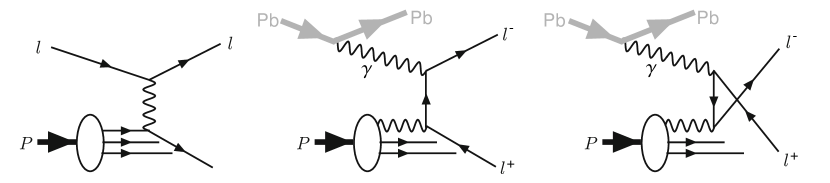
Figure 1: Schematic graphs for deep inelastic scattering, $\ell^{\pm}p\rightarrow\ell^{\pm}+X$ (a) and photon-induced dilepton prodcution, $\gamma p\rightarrow\ell^{+}\ell^{-}+X$, in $p+\textrm{Pb}$ collisions for $t$-channel (b) and $u$-channel (c) lepton exchange.

Moreover, as this process does not involve the exchange of color with the photon-emitting nucleus, no significant particle production is expected in the rapidity region between the dilepton system and the nucleus. The photon-emitting nucleus is also expected to produce no neutrons because the photons couple to the entire nucleus. Thus a combination of requirements on rapidity gap and zero neutrons in the same direction provide straightforward criteria to identify these events experimentally.

II Formalism

II.1 Elastic photon fluxes

To get the distribution of the elastic photons from the proton, one can express the equivalent photon flux through the electric and magnetic form factors $G_{E}(Q^{2})$ and $G_{M}(Q^{2})$ of the proton. This contribution is obtained as

$$\gamma^{p}_{el}(x,Q^{2})=\frac{\alpha_{\rm{em}}}{\pi}\Big{[}\Big{(}1-{x\over 2}\Big{)}^{2}\,{4m_{p}^{2}G_{E}^{2}(Q^{2})+Q^{2}G_{M}^{2}(Q^{2})\over 4m_{p}^{2}+Q^{2}}+{x^{2}\over 4}G_{M}^{2}(Q^{2})\Big{]}\leavevmode\nobreak\ ,$$ (1)

where $x$ is the momentum fraction of the proton taken by the photon, $Q^{2}$ is the photon virtuality, $\alpha_{\rm{em}}$ is the electromagnetic structure constant and $m_{p}$ is the proton mass.

To express the elastic photon flux for the nucleus ($\gamma^{\rm Pb}_{el}$), we follow Ref. Budnev:1974de and replace

$${4m_{p}^{2}G_{E}^{2}(Q^{2})+Q^{2}G_{M}^{2}(Q^{2})\over 4m_{p}^{2}+Q^{2}}\longrightarrow Z^{2}F_{\rm em}^{2}(Q^{2})\leavevmode\nobreak\ ,$$ (2)

where $F_{\rm em}(Q^{2})$ is the electromagnetic form factor of the nucleus and $Z$ is its charge. We also neglect the magnetic form factor of the ion in the following.

For the Pb nucleus, we use the form factor parameterization from the STARlight MC generator Klein:2016yzr :

$$F_{\rm em}(Q^{2})={3\over(QR_{A})^{3}}\Big{[}\sin(QR_{A})-QR_{A}\cos(QR_{A})\Big{]}{1\over 1+a^{2}Q^{2}}\leavevmode\nobreak\ ,$$ (3)

where $R_{A}=1.1A^{1/3}$ fm, $a=0.7$ fm and $Q=\sqrt{Q^{2}}$.

The elastic photon PDFs of the proton and lead nucleus can be integrated over $Q^{2}$ as

$$\gamma^{(p,Pb)}_{el}(x)=\int dQ^{2}\gamma^{(p,Pb)}_{el}(x,Q^{2})\,.$$ (4)

This is useful for the collinear-factorization approach since the $Q^{2}$ dependence factorizes in this case.

II.2 Collinear-factorization approach and choice of the scale

The inelastic processes, with breakup of a proton, can be also considered. At LO and at a given scale $\mu^{2}$, the photon parton distribution $\gamma^{p}_{inel}(x,\mu^{2})$ of photons carrying a fraction $x$ of the proton’s momentum, obeys the DGLAP equation:

$${d\gamma^{p}_{inel}(x,\mu^{2})\over d\log\mu^{2}}= {\alpha_{\rm{em}}\over 2\pi}\int_{x}^{1}{dy\over y}\Big{[}\sum_{q}P_{\gamma\leftarrow q}(y)q({x\over y},\mu^{2})+P_{\gamma\leftarrow\gamma}(y)\gamma^{p}_{inel}({x\over y},\mu^{2})\Big{]}\leavevmode\nobreak\ ,$$ (5)

where $q(x,\mu^{2})$ is the quark PDF, $P_{\gamma\leftarrow q}$ is the $q\rightarrow\gamma$ splitting function, and $P_{\gamma\leftarrow\gamma}$ corresponds to the virtual self-energy correction to the photon propagator. This is the basis for colinear photon-PDFs in the initial Gluck:2002fi ; Martin:2004dh and more recent Ball:2013hta ; Martin:2014nqa ; Schmidt:2014aba ; Harland-Lang:2016kog ; Giuli:2017oii ; Manohar:2016nzj ; Bertone:2017bme analyses.

The computation of the photon-induced dilepton production cross section requires definition of the scale ($\mu^{2}$) at which the photon PDFs are convoluted. The usual choice for $\mu$ is the mass of the system (motivated by the $s$-channel quark–antiquark annihilation process) or the transverse momentum of the leading object. These choices are however not optimal for the $t$- and $u$-channel initiated photon-induced process. By analogy to DIS (Fig. 1), where the scale is associated with the virtuality of the exchanged photon, it is possible to define the scale in case of the $\gamma\gamma\rightarrow\ell^{+}\ell^{-}$ process. This is achieved by taking the virtuality of the massive $t$- or $u$-channel propagator (Fig. 1b or c). Hence, $\mu^{2}=-(p^{\gamma^{Pb}}-p^{\ell^{-}})^{2}$ for the $t$-channel diagram and $\mu^{2}=-(p^{\gamma^{Pb}}-p^{\ell^{+}})^{2}$ for the $u$-channel exchange, where $p^{\gamma^{Pb}}$ is the four momentum of the photon emitted by lead and $p^{\ell^{\pm}}$ is the four momentum of the lepton of the corresponding charge. Note that the $u$- and $t$- channel diagrams have vanishing interference in the zero lepton mass limit. Therefore, they can be separated while convoluting PDFs with the partonic cross section.

In the collinear approach, the $p+\textrm{Pb}\rightarrow\textrm{Pb}+\ell^{+}\ell^{-}+X$ production cross section can be written as

$$\sigma=S^{2}\int dx_{p}dx_{\rm Pb}\Big{[}\gamma^{p}_{el}(x_{p})+\gamma^{p}_{inel}(x_{p},\mu^{2})\Big{]}\gamma^{\rm Pb}_{el}(x_{\rm Pb})\sigma_{\gamma\gamma\rightarrow\ell^{+}\ell^{-}}(x_{p},x_{\rm Pb})\,,$$ (6)

where $\sigma_{\gamma\gamma\rightarrow\ell^{+}\ell^{-}}$ is the elementary cross section for the $\gamma\gamma\rightarrow\ell^{+}\ell^{-}$ subprocess and $S^{2}$ is the so-called survival factor which takes into account the requirement that there be no hadronic interactions between the proton and the ion.

II.3 $k_{T}$-factorization approach

At lowest order, the calculations with collinear photons produce leptons that are back-to-back in transverse kinematics. The transverse momentum appears at higher orders, however to describe full transverse momentum spectrum one needs to match the calculations to resummation or dedicated parton shower algorithms. This approach is not considered in this paper.

In the $k_{T}$ factorization approach (also named as high-energy factorization), one can parametrize the $\gamma^{*}p\rightarrow X$ vertices in terms of the proton structure functions. The photons from inelastic production have transverse momenta and non-zero virtualities $Q^{2}$ and the unintegrated photon distributions are used, in contrast to collinear distributions. In the DIS limit, the unintegrated inelastic photon flux can be obtained using the following equation daSilveira:2014jla ; Luszczak:2015aoa :

$$\gamma^{p}_{inel}(x,Q^{2})={1\over x}{1\over\pi Q^{2}}\,\int_{M^{2}_{\rm thr}}dM_{X}^{2}{\cal{F}}^{\mathrm{in}}_{\gamma^{*}\leftarrow p}(x,\vec{q}_{T}^{2},M^{2}_{X})\,,$$ (7)

and we use the functions ${\cal{F}}^{\mathrm{in}}_{\gamma^{*}\leftarrow p}$ from Budnev:1974de ; Luszczak:2018ntp :

$${\cal{F}}^{\mathrm{in}}_{\gamma^{*}\leftarrow p}(x,\vec{q}_{T}^{2},M_{X}) = {\alpha_{\rm em}\over\pi}\Big{\{}(1-x)\Big{(}{\vec{q}_{T}^{2}\over\vec{q}_{T}^{2}+x(M_{X}^{2}-m_{p}^{2})+x^{2}m_{p}^{2}}\Big{)}^{2}{F_{2}(x_{\rm Bj},Q^{2})\over Q^{2}+M_{X}^{2}-m_{p}^{2}}$$ (8)

$$+ {x^{2}\over 4x^{2}_{\rm Bj}}{\vec{q}_{T}^{2}\over\vec{q}_{T}^{2}+x(M_{X}^{2}-m_{p}^{2})+x^{2}m_{p}^{2}}{2x_{\rm Bj}F_{1}(x_{\rm Bj},Q^{2})\over Q^{2}+M_{X}^{2}-m_{p}^{2}}\Big{\}}\,.$$

The virtuality $Q^{2}$ of the photon depends on the photon transverse momentum ($\vec{q}_{T}^{2}$) and the proton remnant mass ($M_{X}$):

$$Q^{2}={\vec{q}_{T}^{2}+x(M_{X}^{2}-m_{p}^{2})+x^{2}m_{p}^{2}\over(1-x)}\,.$$ (9)

Moreover, the proton structure functions $F_{1}(x_{\rm Bj},Q^{2})$ and $F_{2}(x_{\rm Bj},Q^{2})$ require the argument

$$x_{\rm Bj}={Q^{2}\over Q^{2}+M^{2}_{X}-m_{p}^{2}}.$$ (10)

Note that in Eq. 8 instead of using $F_{2}(x_{\rm Bj},Q^{2}),F_{1}(x_{\rm Bj},Q^{2})$, we in practice use the pair $F_{2}(x_{\rm Bj},Q^{2}),F_{L}(x_{\rm Bj},Q^{2})$, where

$$F_{L}(x_{\rm Bj},Q^{2})=\Big{(}1+{4x_{\rm Bj}^{2}m_{p}^{2}\over Q^{2}}\Big{)}F_{2}(x_{\rm Bj},Q^{2})-2x_{\rm Bj}F_{1}(x_{\rm Bj},Q^{2})$$ (11)

is the longitudinal structure function of the proton.

These unintegrated photon fluxes enter the $p+\textrm{Pb}\rightarrow\textrm{Pb}+\ell^{+}\ell^{-}+X$ production cross section as

$$\sigma=S^{2}\int dx_{p}dx_{\rm Pb}d\vec{q}_{T}\Big{[}\gamma^{p}_{el}(x_{p},Q^{2})+\gamma^{p}_{inel}(x_{p},Q^{2})\Big{]}\gamma^{\rm Pb}_{el}(x_{\rm Pb})\sigma_{\gamma^{*}\gamma\rightarrow\ell^{+}\ell^{-}}(x_{p},x_{\rm Pb},\vec{q_{T}})\,,$$ (12)

where $\sigma_{\gamma^{*}\gamma\rightarrow\ell^{+}\ell^{-}}$ is the off-shell elementary cross-section (for details see Refs. daSilveira:2014jla ; Catani:1990eg ) and for $x_{p}\ll 1$ we have $Q^{2}\approx\vec{q}_{T}^{2}$ (see Eq. 9). One should note that while the fluxes do not depend on the direction of $\vec{q}_{T}$, averaging over directions of $\vec{q}_{T}$ in the off-shell cross section replaces the average over photon polarizations in the collinear case.

III Example experimental configuration and possible background sources

We assume collision setup from recent $p+\textrm{Pb}$ run at the LHC, carried out at the centre-of-mass energy per nucleon pair $\sqrt{s_{NN}}=8.16$ TeV. Since the energy per nucleon in the proton beam is larger than in the lead beam, the nucleon–nucleon centre-of-mass system has a rapidity in the laboratory frame of $y=0.465$.

As an example of method’s applicability, we will use the geometry of ATLAS Aad:2008zzm and CMS Chatrchyan:2008aa detectors in the following. We consider only the dimuon channel, however the integrated results for $ee$ and $\mu\mu$ channels can be obtained by simply multiplying the dimuon cross-sections by a factor of two.

We start by applying a minimum transverse momentum requirement of 4 GeV to both muons. This requirement is imposed to ensure high lepton reconstruction and triggering efficiency. Moreover, due to limited acceptance of the detectors, each muon is required to have a pseudorapidity ($\eta^{\ell}$) that satisfies $|\eta^{\ell}|<2.4$. Our calculations are carried out for a minimum dilepton invariant mass of $m_{\ell^{+}\ell^{-}}=10$ GeV. Such a choice is due to removal of possible contamination from $\Upsilon(\rightarrow\ell^{+}\ell^{-})$ photoproduction. A summary of all selection requirements is presented in Table 1.

Variable	Requirement
lepton transverse momentum, $p_{\textrm{T}}^{\ell}$	$>4$ GeV
lepton pseudorapidity, $|\eta^{\ell}|$	$<2.4$
dilepton invariant mass, $m_{\ell^{+}\ell^{-}}$	$>10$ GeV

Table 1: Definition of the fiducial region used in the studies.

Possible background for this process can arise from inclusive lepton-pair production, e.g. from Drell–Yan process Drell:1970wh ; Aad:2015gta ; Khachatryan:2015pzs ; Alice:2016wka . This processes would lead to disintegration of the incoming ion, and zero-degree calorimeters (ZDC) Dellacasa:1999ke ; ATLAS:2007aa can be used to veto very-forward-going neutral fragments which would allow this background to be reduced fully. Another background can arise from diffractive interactions, hence possibly mimicking the signal topology. However, since the Pb nucleus is a fragile object (with the nucleon binding energy of just 8 MeV) even the softest diffractive interaction will likely result in the emission of a few nucleons from the ion, detectable in the ZDC.

Another background category is the photon-induced process with a resolved photon, i.e. $\gamma p\rightarrow Z/\gamma^{*}+X$ reaction. Here, the rapidity gap is expected to be smaller than in the signal process due to the additional particle production associated with the “photon remnant”. Any other residual contamination of this process can be controlled using a dedicated sample, with a dilepton invariant mass around the $Z$-boson mass.

IV Results with collinear photon-PDFs

We start with the calculation of the elastic contribution, $p+\textrm{Pb}\rightarrow p+\textrm{Pb}+\ell^{+}\ell^{-}$ for which the following parameterization is used Budnev:1974de :

$$\gamma^{p}_{el}(x)=\frac{\alpha_{\rm em}}{\pi}\left(\frac{1-x+0.5x^{2}}{x}\right)\left(\frac{F+3}{F-1}\log{F}-\frac{17}{6}-\frac{4}{3F}+\frac{1}{6F^{2}}\right)\leavevmode\nobreak\ ,$$ (13)

where $F=1+\frac{Q_{0}^{2}(1-x)}{x^{2}m_{p}^{2}}$ and $Q_{0}^{2}=0.71$ GeV². This parameterization is a good analytical approximation of Eq. 1 integrated over $Q^{2}$. The results for the elastic case are cross-checked with the calculation from STARlight MC and a good agreement between the fiducial cross-sections is found: $\sigma_{fid}^{\textrm{el}}=17.5$ nb, whereas $\sigma_{fid}^{\textrm{STARlight}}=17.0$ nb. Both calculations are also corrected by a factor $S^{2}=0.96$ which is calculated using STARlight, where the hard-sphere proton–nucleus requirement Klein:2016yzr is used.

Next, for the inelastic case ($\gamma p\rightarrow\ell^{+}\ell^{-}+X$), several recent parameterizations of the photon parton distributions are studied: CT14qed Schmidt:2015zda , HKR16qed Harland-Lang:2016kog , LUXqed17 Manohar:2017eqh and NNPDF3.1luxQED Bertone:2017bme . All predictions are scaled by $S^{2}=0.95$, again derived from STARlight. This value of $S^{2}$ is lower than for the purely elastic case, due to slightly smaller average impact parameter between the proton and the ion in the inelastic reaction. One should note that all of these PDF sets include both elastic and inelastic parts of the photon spectrum. We keep the elastic part now (as provided by each group), but we subtract it later in Sec. VI for the comparison with $k_{T}$-factorization results.

The integrated fiducial cross-sections for $p+\textrm{Pb}\rightarrow\textrm{Pb}+\ell^{+}\ell^{-}+X$ production at $\sqrt{s_{NN}}=8.16$ TeV for different collinear photon PDF sets are summarized in Tab. 2. Comparison of several lepton kinematic distributions between different photon-PDFs is shown in Fig. 2, including invariant mass and rapidity of lepton pair, and single-lepton transverse momentum/pseudorapidity distributions. The asymmetry visible in pair rapidity and single-lepton pseudorapidity distributions is due to expermental setup, which assumes a difference in the energy per nucleon between the proton beam and the lead beam (see Sec. III). All photon PDF parameterizations agree within 20% with each other. The differences are mainly due to overall PDF normalization, as no variation in the shape of various kinematic distributions is observed.

To check the sensitivity to the nuclear form factor modelling (Eq. 3), different values of $R_{A}$ ($R_{A}=7.1$ fm) and $a$ ($a=0.55$ fm) parameters are used, in a similar way as in Ref. Azevedo:2019fyz . These variations change the fiducial cross-sections by 4% and 3% respectively.

Contribution	$p_{T}^{\ell}>4$ GeV	$p_{T}^{\ell}>4$ GeV, $|\eta^{\ell}|<2.4$,
		$m_{\ell^{+}\ell^{-}}>10$ GeV
$\gamma^{p}_{\rm{el}}$	44.9 nb	17.5 nb
$\gamma^{p}_{\rm{el}}+\gamma^{p}_{\rm{inel}}$ [CT14qed_inc]	$98\pm 4$ (PDF) nb	$40\pm 2$ (PDF) nb
$\gamma^{p}_{\rm{el}}+\gamma^{p}_{\rm{inel}}$ [LUXqed17]	$105.8\pm 0.2$ (PDF) nb	$44.1\pm 0.1$ (PDF) nb
$\gamma^{p}_{\rm{el}}+\gamma^{p}_{\rm{inel}}$ [NNPDF3.1luxQED]	$115.6\pm 0.6$ (PDF) nb	$45.9\pm 0.3$ (PDF) nb
$\gamma^{p}_{\rm{el}}+\gamma^{p}_{\rm{inel}}$ [HKR16qed]	121.6 nb	49.4 nb

Table 2: Integrated fiducial cross sections for $p+\textrm{Pb}\rightarrow\textrm{Pb}+\ell^{+}\ell^{-}+X$ production at $\sqrt{s_{NN}}=8.16$ TeV for different collinear photon PDF sets. The effect of applying only $p_{T}^{\ell}$ requirement is shown in second column. The uncertainties denote the PDF uncertainties (if available) calculated at 68% CL. For comparison, the cross section for purely elastic contribution is also shown.

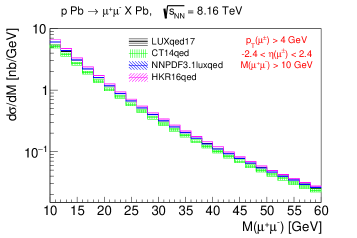
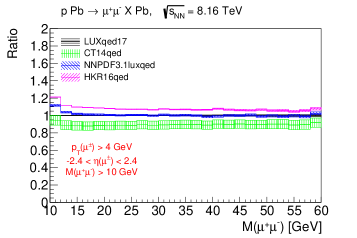
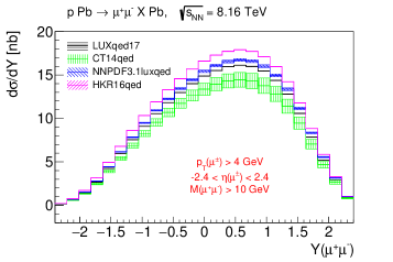
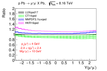
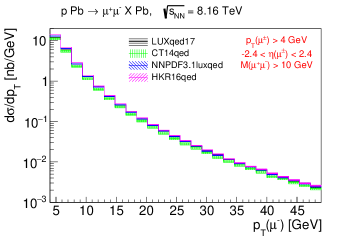
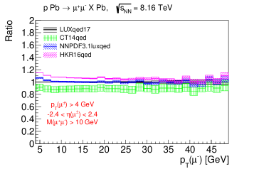
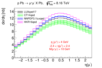
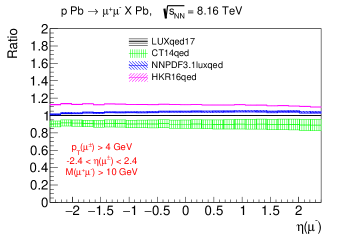
Figure 2: Differential cross sections in the fiducial region for $p+\textrm{Pb}\rightarrow\textrm{Pb}+\ell^{+}\ell^{-}+X$ production at $\sqrt{s_{NN}}=8.16$ TeV for different collinear photon PDF sets. Four differential distributions are shown (from top to bottom): invariant mass of lepton pair, pair rapidity, transverse momentum of negatively-charged lepton and its pseudorapidity. Figures on the right show the ratios to LUXqed17 PDF. The bands denote the PDF uncertainties (if available) calculated at 68% CL, and the statistical uncertainties of the calculations added in quadrature.

V Results using $k_{T}$-factorization approach

Several different parametrizations of proton strucure functions are used. Those are labeled as:

• ALLM Abramowicz:1991xz ; Abramowicz:1997ms : This parametrization gives a good fit to $F_{2}$ in most of the measured regions.

• SY Suri:1971yx : This parameterization of Suri and Yennie from the early 1970’s does not include DGLAP evolution. It is still used as one of the defaults in the LPAIR event generator Vermaseren:1982cz .

• SU Szczurek:1999rd : A parametrization which concentrates to give a good description at small and intermediate $Q^{2}$ for $x>0.01$. At large $Q^{2}$, it is complemented by the NNLO calculation of $F_{2}$ and $F_{L}$ from NNLO MSTW 2008 PDF analysis Martin:2009iq .

• LUX-like: a recently constructed parametrization, described in details in Ref. Luszczak:2018ntp . This setup closely follows the LUXqed work from Ref.Manohar:2017eqh .

To model $\gamma^{p}_{el}(x,Q^{2})$ we use Eq. 1 with so-called dipole parametrization of the proton form factors:

$$G_{E}(Q^{2}) = \left(1+\frac{Q^{2}}{Q_{0}^{2}}\right)^{-2}$$ (14)

$$G_{M}(Q^{2}) = \mu_{p}G_{E}(Q^{2})\leavevmode\nobreak\ ,$$ (15)

where $\mu_{p}$ is the proton magnetic moment.

Table 3 shows the comparison of integrated fiducial cross sections for inelastic $p+\textrm{Pb}\rightarrow\textrm{Pb}+\ell^{+}\ell^{-}+X$ production at $\sqrt{s_{NN}}=8.16$ TeV for different proton structure functions. All structure functions provide similar fiducial cross-section, at the level of 16–18 nb. These inelastic cross-sections are also similar in size to the elastic contribution (18 nb) and are slightly lower than the numbers from collinear analysis, subtracted for elastic part (see Table 2). A comparison is also made with LUX-like parametrization when the longitudinal structure function ($F_{L}$) is explicitly considered. This leads to the decrease of the cross section by 2%, similarly to Ref. Luszczak:2018ntp .

Figure 3 presents differential cross sections for several lepton kinematic distributions: invariant mass of lepton pair, leading lepton transverse momentum, lepton pseudorapidity difference and leading lepton pseudorapidity. The shapes of the distributions obtained with various proton structure functions are very similar. For completeness, differential cross sections as a function of lepton pair transverse momentum and azimuthal angle difference between the pair are shown in Fig. 4. Quite large (small) transverse momenta (angle differences) are possible, in contrast to leading-order calculations with collinear photons where the corresponding distributions are just Dirac delta functions. The $k_{T}$-factorization approach should be considered more appropriate here. It is also visible that the SY parametrization gives lower predictions at larger pair-$p_{T}$, comparing to the other parametrizations used. This is because SY parametrization does not include explicit DGLAP evolution terms, which are relevant for large photon virtualities.

Based on Fig. 4, it is also possible to separate experimentally the elastic part ($p+\textrm{Pb}\rightarrow p+\textrm{Pb}+\ell^{+}\ell^{-}$), with striking back-to-back topology, from the inelastic contribution. With $k_{T}$-factorization, one can also calculate the mass of the proton remnants ($M_{X}$). This is shown in Fig. 5; in contrast to the elastic case ($M_{X}=m_{p}$) quite large masses of the remnant system can be achieved.

Contribution	$p_{T}^{\ell}>4\leavevmode\nobreak\ \text{Ge\kern-1.00006ptV}$	$p_{T}^{\ell}>4\leavevmode\nobreak\ \text{Ge\kern-1.00006ptV}$, $|\eta^{\ell}|<2.4$, $m_{\ell^{+}\ell^{-}}>10\leavevmode\nobreak\ \text{Ge\kern-1.00006ptV}$
$\gamma^{p}_{\rm{el}}$	47.9 nb	18.3 nb
$\gamma^{p}_{\rm{inel}}$ [LUX-like $F_{2}$]	43.6 nb	17.4 nb
$\gamma^{p}_{\rm{inel}}$ [LUX-like $F_{2}+F_{L}$]	42.6 nb	17.1 nb
$\gamma^{p}_{\rm{inel}}$ [ALLM97 $F_{2}$]	41.7 nb	16.4 nb
$\gamma^{p}_{\rm{inel}}$ [SU $F_{2}$]	41.7 nb	16.7 nb
$\gamma^{p}_{\rm{inel}}$ [SY $F_{2}$]	40.4 nb	16.0 nb

Table 3: Integrated fiducial cross sections for inelastic $p+\textrm{Pb}\rightarrow\textrm{Pb}+\ell^{+}\ell^{-}+X$ production at $\sqrt{s_{NN}}=8.16$ TeV for different proton structure functions. The effect of applying only $p_{T}^{\ell}$ requirement is shown in second column.

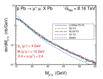
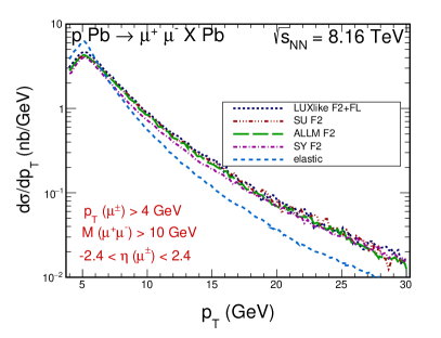
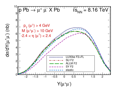
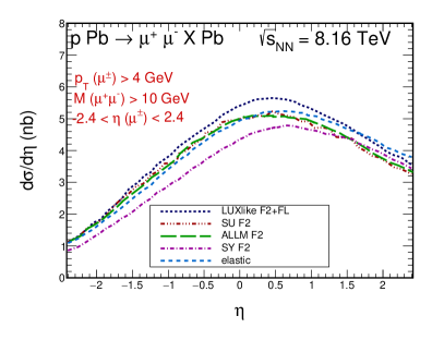
Figure 3: Differential cross sections in the fiducial region for $p+\textrm{Pb}\rightarrow\textrm{Pb}+\ell^{+}\ell^{-}+X$ production at $\sqrt{s_{NN}}=8.16$ TeV in $k_{T}$ factorization approach for several proton structure functions. Four differential distributions are shown: invariant mass of lepton pair (top left), leading lepton transverse momentum (top right), dilepton rapidity (bottom left) and leading lepton pseudorapidity (bottom right). For comparison, the elastic contribution ($p+\textrm{Pb}\rightarrow p+\textrm{Pb}+\ell^{+}\ell^{-}$) is also shown.

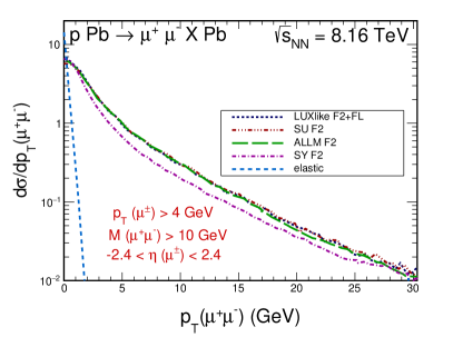
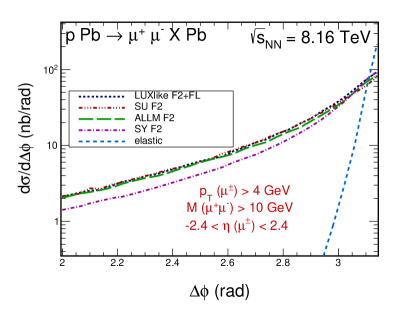
Figure 4: Differential cross sections in the fiducial region for $p+\textrm{Pb}\rightarrow\textrm{Pb}+\ell^{+}\ell^{-}+X$ production at $\sqrt{s_{NN}}=8.16$ TeV in $k_{T}$ factorization approach for several proton structure functions. Two differential distributions are shown: transverse momentum of lepton pair (left) and azimuthal angle difference between the pair (right). For comparison, the elastic contribution ($p+\textrm{Pb}\rightarrow p+\textrm{Pb}+\ell^{+}\ell^{-}$) is also shown.

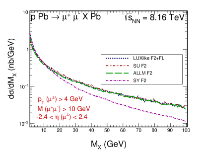
Figure 5: Differential cross section as a function of the mass of the proton remnants in the fiducial region for $p+\textrm{Pb}\rightarrow\textrm{Pb}+\ell^{+}\ell^{-}+X$ production at $\sqrt{s_{NN}}=8.16$ TeV in $k_{T}$ factorization approach for several proton structure functions.

VI Discussion

Figure 6 compares several differential distributions computed using the two approaches. For the collinear approach pure inelastic contribution is estimated by subtracting elastic part computed following Eq. 13. For the invariant mass distribution and lepton pseudorapidity the shapes are similar and the main difference between the two predictions is observed in the normalization. For the distribution of the lepton pair rapidity the two predictions agree at larger rapidities while disagreement concentrates in the central region. The biggest difference is observed for the transverse momentum distribution of the lepton where at low $p_{T}$ collinear approximation exceeds the estimate from $k_{T}$-factorization approach while at high $p_{T}$ the ordering is reversed. This suggests that at low $p_{T}$ (close to the boundary of the fiducial region) the difference is due to the smearing of dilepton transverse momentum introduced by the $k_{T}$-factorization approach.

We also take the opportunity to calculate expected number of events for realistic assumption on total integrated luminosity. Based on the previous $p+\textrm{Pb}$ runs at the LHC, we assume $\int Ldt=200\leavevmode\nobreak\ \textrm{nb}^{-1}$. We also assume possible experimental efficiencies, mainly due to trigger and reconstruction of leptons, which we embed in a single correction factor $C=0.7$.

Table 4 shows the expected number of events for $p+\textrm{Pb}\rightarrow\textrm{Pb}+\ell^{+}\ell^{-}+X$ production at $\sqrt{s_{NN}}=8.16$ TeV and configuration described above. Approximately 2500 elastic dilepton events are expected. Depending on the calculations, 3400 (collinear with LUXqed17 PDF) or 2400 ($k_{T}$-factorization with LUX-like $F_{2}+F_{L}$) reconstructed inelastic events are predicted. The data should be therefore sensitive to discriminate between the predictions based on collinear and $k_{T}$-factorization approaches, using existing datasets collected by ATLAS and CMS.

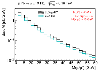
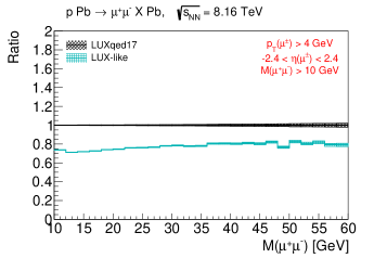
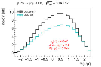
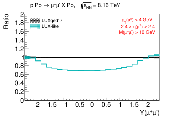
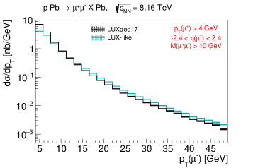
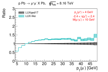
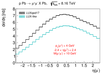
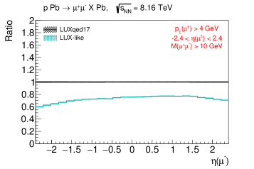
Figure 6: Differential cross sections in the fiducial region for $p+\textrm{Pb}\rightarrow\textrm{Pb}+\ell^{+}\ell^{-}+X$ production at $\sqrt{s_{NN}}=8.16$ TeV for collinear LUXqed17 photon PDF and for LUX-like $F_{2}+F_{L}$ photon PDF with $k_{T}$-factorization. Four differential distributions are shown (from top to bottom): invariant mass of lepton pair, pair rapidity, transverse momentum of negatively-charged lepton and its pseudorapidity. Figures on the right show the ratios to LUXqed17 PDF.

Contribution	Expected events ($C=1$)	Expected events ($C=0.7$)
$\gamma^{p}_{\rm{el}}$	3600	2500
$\gamma^{p}_{\rm{inel}}$ [LUXqed17 collinear]	5600	3900
$\gamma^{p}_{\rm{inel}}$ [LUX-like $F_{2}+F_{L}$]	3400	2400

Table 4: Expected number of events for $p+\textrm{Pb}\rightarrow\textrm{Pb}+\ell^{+}\ell^{-}+X$ production at $\sqrt{s_{NN}}=8.16$ TeV assuming $\int Ldt=200\leavevmode\nobreak\ \textrm{nb}^{-1}$. Shown are several contributions: purely elastic, inelastic with collinear LUXqed17 PDF and inelastic with $k_{T}$-factorization and LUX-like $F_{2}+F_{L}$ proton structure function parameterization. An effect of possible experimental efficiencies is shown in last column.

VII Summary

In summary, we propose a method that would provide an unambiguous test of the photon parton distribution at LHC energies, and allow constraints to be placed on it. This method is based on the measurement of the cross-section for the reaction $p+\textrm{Pb}\rightarrow\textrm{Pb}+\ell^{+}\ell^{-}+X$, where the expected background is small compared to the analogous process in $pp$ collisions. Results are shown for different choices of collinear photon PDFs, and a comparison is made with unintegrated photon distributions that include non-zero photon transverse momentum. Due to the smearing of dilepton transverse momentum introduced by the $k_{T}$-factorization approach, these two approaches lead to the cross sections that differ by about 30%. Moreover, for collinear approach and by analogy to DIS, an optimal choice of the scale is identified. Using simple (realistic) experimental requirements on lepton kinematics, it is shown that one can expect O(3000) inelastic events with the existing datasets recorded by ATLAS/CMS at $\sqrt{s_{NN}}=8.16$ TeV for each lepton flavour.

References

References

- (1) ATLAS Collaboration, G. Aad et al., Measurement of the low-mass Drell-Yan differential cross section at = 7 TeV using the ATLAS detector, JHEP 06 (2014) 112, arXiv:1404.1212 [hep-ex].
- (2) ATLAS Collaboration, G. Aad et al., Measurement of the double-differential high-mass Drell-Yan cross section in pp collisions at TeV with the ATLAS detector, JHEP 08 (2016) 009, arXiv:1606.01736 [hep-ex].
- (3) E. Accomando, J. Fiaschi, F. Hautmann, S. Moretti, and C. H. Shepherd-Themistocleous, Photon-initiated production of a dilepton final state at the LHC: Cross section versus forward-backward asymmetry studies, Phys. Rev. D95 (2017) no. 3, 035014, arXiv:1606.06646 [hep-ph].
- (4) M. Luszczak, W. Schafer, and A. Szczurek, Two-photon dilepton production in proton-proton collisions: two alternative approaches, Phys. Rev. D93 (2016) no. 7, 074018, arXiv:1510.00294 [hep-ph].
- (5) L. A. Harland-Lang, V. A. Khoze, and M. G. Ryskin, The photon PDF in events with rapidity gaps, Eur. Phys. J. C76 (2016) no. 5, 255, arXiv:1601.03772 [hep-ph].
- (6) M. Luszczak, A. Szczurek, and C. Royon, pair production in proton-proton collisions: small missing terms, JHEP 02 (2015) 098, arXiv:1409.1803 [hep-ph].
- (7) A. Denner, S. Dittmaier, M. Hecht, and C. Pasold, NLO QCD and electroweak corrections to production with leptonic Z-boson decays, JHEP 02 (2016) 057, arXiv:1510.08742 [hep-ph].
- (8) M. Dyndal and L. Schoeffel, Four-lepton production from photon-induced reactions in collisions at the LHC, Acta Phys. Polon. B47 (2016) 1645, arXiv:1511.02065 [hep-ph].
- (9) P. Obul, M. Ababekri, S. Dulat, J. Isaacson, C. Schmidt, and C. P. Yuan, Implications of CMS analysis of photon-photon interactions for photon PDFs, Chin. Phys. C42 (2018) no. 11, 113101, arXiv:1603.04874 [hep-ph].
- (10) B. Biedermann, M. Billoni, A. Denner, S. Dittmaier, L. Hofer, B. Jäger, and L. Salfelder, Next-to-leading-order electroweak corrections to 4 leptons at the LHC, JHEP 06 (2016) 065, arXiv:1605.03419 [hep-ph].
- (11) B. Biedermann, A. Denner, S. Dittmaier, L. Hofer, and B. Jäger, Electroweak corrections to at the LHC: a Higgs background study, Phys. Rev. Lett. 116 (2016) no. 16, 161803, arXiv:1601.07787 [hep-ph].
- (12) Y. Wang, R.-Y. Zhang, W.-G. Ma, X.-Z. Li, and L. Guo, QCD and electroweak corrections to ZZ+jet production with Z -boson leptonic decays at the LHC, Phys. Rev. D94 (2016) no. 1, 013011, arXiv:1604.04080 [hep-ph].
- (13) M. Luszczak, W. Schafer, and A. Szczurek, Production of pairs via subprocess with photon transverse momenta, JHEP 05 (2018) 064, arXiv:1802.03244 [hep-ph].
- (14) A. Manohar, P. Nason, G. P. Salam, and G. Zanderighi, How bright is the proton? A precise determination of the photon parton distribution function, Phys. Rev. Lett. 117 (2016) no. 24, 242002, arXiv:1607.04266 [hep-ph].
- (15) C. Schmidt, J. Pumplin, D. Stump, and C. P. Yuan, CT14QED parton distribution functions from isolated photon production in deep inelastic scattering, Phys. Rev. D93 (2016) no. 11, 114015, arXiv:1509.02905 [hep-ph].
- (16) NNPDF Collaboration, R. D. Ball, V. Bertone, S. Carrazza, L. Del Debbio, S. Forte, A. Guffanti, N. P. Hartland, and J. Rojo, Parton distributions with QED corrections, Nucl. Phys. B877 (2013) 290–320, arXiv:1308.0598 [hep-ph].
- (17) xFitter Developers’ Team Collaboration, F. Giuli et al., The photon PDF from high-mass Drell-Yan data at the LHC, Eur. Phys. J. C77 (2017) no. 6, 400, arXiv:1701.08553 [hep-ph].
- (18) ATLAS Collaboration, G. Aad et al., Measurement of exclusive production in proton-proton collisions at TeV with the ATLAS detector, Phys. Lett. B749 (2015) 242–261, arXiv:1506.07098 [hep-ex].
- (19) ATLAS Collaboration, M. Aaboud et al., Measurement of the exclusive process in proton-proton collisions at TeV with the ATLAS detector, Phys. Lett. B777 (2018) 303–323, arXiv:1708.04053 [hep-ex].
- (20) CMS Collaboration, S. Chatrchyan et al., Exclusive photon-photon production of muon pairs in proton-proton collisions at TeV, JHEP 01 (2012) 052, arXiv:1111.5536 [hep-ex].
- (21) CMS Collaboration, S. Chatrchyan et al., Search for exclusive or semi-exclusive photon pair production and observation of exclusive and semi-exclusive electron pair production in collisions at TeV, JHEP 11 (2012) 080, arXiv:1209.1666 [hep-ex].
- (22) CMS, TOTEM Collaboration, A. M. Sirunyan et al., Observation of proton-tagged, central (semi)exclusive production of high-mass lepton pairs in pp collisions at 13 TeV with the CMS-TOTEM precision proton spectrometer, JHEP 07 (2018) 153, arXiv:1803.04496 [hep-ex].
- (23) V. M. Budnev, I. F. Ginzburg, G. V. Meledin, and V. G. Serbo, The two photon particle production mechanism. Physical problems. Applications. Equivalent photon approximation, Phys. Rept. 15 (1975) 181.
- (24) S. R. Klein, J. Nystrand, J. Seger, Y. Gorbunov, and J. Butterworth, STARlight: A Monte Carlo simulation program for ultra-peripheral collisions of relativistic ions, Comput. Phys. Commun. 212 (2017) 258–268, arXiv:1607.03838 [hep-ph].
- (25) M. Gluck, C. Pisano, and E. Reya, The Polarized and unpolarized photon content of the nucleon, Phys. Lett. B540 (2002) 75–80, arXiv:hep-ph/0206126 [hep-ph].
- (26) A. D. Martin, R. G. Roberts, W. J. Stirling, and R. S. Thorne, Parton distributions incorporating QED contributions, Eur. Phys. J. C39 (2005) 155–161, arXiv:hep-ph/0411040 [hep-ph].
- (27) A. D. Martin and M. G. Ryskin, The photon PDF of the proton, Eur. Phys. J. C74 (2014) 3040, arXiv:1406.2118 [hep-ph].
- (28) C. Schmidt, J. Pumplin, D. Stump, and C. P. Yuan, QED effects and Photon PDF in the CTEQ-TEA Global Analysis, PoS DIS2014 (2014) 054.
- (29) L. A. Harland-Lang, V. A. Khoze, and M. G. Ryskin, Photon-initiated processes at high mass, Phys. Rev. D94 (2016) no. 7, 074008, arXiv:1607.04635 [hep-ph].
- (30) NNPDF Collaboration, V. Bertone, S. Carrazza, N. P. Hartland, and J. Rojo, Illuminating the photon content of the proton within a global PDF analysis, SciPost Phys. 5 (2018) 008, arXiv:1712.07053 [hep-ph].
- (31) G. G. da Silveira, L. Forthomme, K. Piotrzkowski, W. Schäfer, and A. Szczurek, Central production via photon-photon fusion in proton-proton collisions with proton dissociation, JHEP 02 (2015) 159, arXiv:1409.1541 [hep-ph].
- (32) S. Catani, M. Ciafaloni, and F. Hautmann, High-energy factorization and small x heavy flavor production, Nucl. Phys. B366 (1991) 135–188.
- (33) ATLAS Collaboration, G. Aad et al., The ATLAS Experiment at the CERN Large Hadron Collider, JINST 3 (2008) S08003.
- (34) CMS Collaboration, S. Chatrchyan et al., The CMS Experiment at the CERN LHC, JINST 3 (2008) S08004.
- (35) S. D. Drell and T.-M. Yan, Massive Lepton Pair Production in Hadron-Hadron Collisions at High-Energies, Phys. Rev. Lett. 25 (1970) 316–320. [Erratum: Phys. Rev. Lett.25,902(1970)].
- (36) ATLAS Collaboration, G. Aad et al., boson production in Pb collisions at TeV measured with the ATLAS detector, Phys. Rev. C92 (2015) no. 4, 044915, arXiv:1507.06232 [hep-ex].
- (37) CMS Collaboration, V. Khachatryan et al., Study of Z boson production in pPb collisions at TeV, Phys. Lett. B759 (2016) 36–57, arXiv:1512.06461 [hep-ex].
- (38) ALICE Collaboration, J. Adam et al., W and Z boson production in p-Pb collisions at = 5.02 TeV, JHEP 02 (2017) 077, arXiv:1611.03002 [nucl-ex].
- (39) ALICE Collaboration, G. Dellacasa et al., ALICE technical design report of the zero degree calorimeter (ZDC), . CERN-LHCC-99-05.
- (40) ATLAS Collaboration, Zero degree calorimeters for ATLAS, . CERN-LHCC-2007-01.
- (41) A. V. Manohar, P. Nason, G. P. Salam, and G. Zanderighi, The Photon Content of the Proton, JHEP 12 (2017) 046, arXiv:1708.01256 [hep-ph].
- (42) C. Azevedo, V. P. Goncalves, and B. D. Moreira, Exclusive dilepton production in ultraperipheral collisions at the LHC, Eur. Phys. J. C79 (2019) no. 5, 432, arXiv:1902.00268 [hep-ph].
- (43) H. Abramowicz, E. M. Levin, A. Levy, and U. Maor, A Parametrization of sigma-T (gamma* p) above the resonance region , Phys. Lett. B269 (1991) 465–476.
- (44) H. Abramowicz and A. Levy, The ALLM parameterization of sigma(tot)(gamma* p): An Update, arXiv:hep-ph/9712415 [hep-ph].
- (45) A. Suri and D. R. Yennie, The space-time phenomenology of photon absorption and inelastic electron scattering, Annals Phys. 72 (1972) 243.
- (46) J. A. M. Vermaseren, Two Photon Processes at Very High-Energies, Nucl. Phys. B229 (1983) 347–371.
- (47) A. Szczurek and V. Uleshchenko, Nonpartonic components in the nucleon structure functions at small in the broad range of x, Eur. Phys. J. C12 (2000) 663–671, arXiv:hep-ph/9904288 [hep-ph].
- (48) A. D. Martin, W. J. Stirling, R. S. Thorne, and G. Watt, Parton distributions for the LHC, Eur. Phys. J. C63 (2009) 189–285, arXiv:0901.0002 [hep-ph].