Game-Theoretic Randomness for Blockchain Games

Abstract

In this paper, we consider the problem of generating fair randomness in a deterministic, multi-agent context (for instance, a decentralised game built on a blockchain). The existing state-of-the-art approaches are either susceptible to manipulation if the stakes are high enough, or they are not generally applicable (specifically for massive game worlds as opposed to games between a small set of players). We propose a novel method based on game theory: By allowing agents to bet on the outcomes of random events against the miners (who are ultimately responsible for the randomness), we are able to align the incentives so that the distribution of random events is skewed only slightly even if miners are trying to maximise their profit and engage in block withholding to cheat in games.

Keywords: Blockchain Gaming, Game Theory, Random-Number Generation, Block Withholding, Huntercoin

1 Introduction

With the creation of Bitcoin [10] in 2008, its pseudonymous inventor Satoshi Nakamoto solved a previously impossible problem: It became possible for fully decentralised P2P networks to reach consensus about the current state of a distributed ledger. This allowed the creation of secure digital money without any trusted intermediary, and was without doubt a revolutionary progress of technology.

But Nakamoto consensus is not limited to building cryptocurrencies like Bitcoin. The same mechanism can be applied to reach consensus about other things as well in a decentralised setting. The first such application was Namecoin [19], where Nakamoto consensus is used to establish who was the first to register a particular name (e.g. a domain name or pseudonym) in the system and who is the “rightful” owner of it. Recently, there has also been a lot of interest and activity in the field of blockchain games, where Nakamoto consensus is applied to an online game. This idea was pioneered by Huntercoin [15] [22] in 2014, and became widely known with the launch of CryptoKitties [6] in 2017.

In this paper, we want to tackle one problem of specific interest in blockchain games: How to produce fair and secure random numbers. By the nature of blockchain systems and the need for a consensus among network participants, all computations need to be deterministic. This includes events in games that are meant to be “random”. Furthermore, since blockchain applications often involve monetary stakes, it is important to produce random numbers in a way that cannot be manipulated or predicated, giving unfair advantages to certain participants in a game.

There are currently two dominant approaches for the generation of random numbers in blockchain games: They can be based off block hashes or a hash-commitment scheme can be used to generate provably-fair random numbers among a well-defined set of players (e.g. a casino and a player). Both methods, however, have certain drawbacks: The first can be manipulated by miners if the stake in a game is high enough; the second is only applicable in some situations and, notably, not to MMO-type games like Huntercoin. This will be discussed in more detail in Section 3.

In Section 4 below, we propose a novel alternative method, which is based on block hashes and generally applicable, but uses a specific betting mechanism to punish dishonest miners. Our game-theoretic analysis in Section 5 shows that this does, indeed, align miner incentives with those of players of a blockchain game. (For the main result, see Theorem 15.) Manipulation of random numbers by miners is strongly discouraged, so that miners are much more honest and the game play will be much fairer for everyone.

2 Blockchain Background

In this section, we want to give a brief overview of the blockchain background that is necessary for the remainder of this paper. A more general description of the basic mechanisms employed by a blockchain using Nakamoto consensus can be found in the seminal paper [10] or the more extensive book [1].

2.1 Proof-of-Work Mining

A blockchain is an append-only data structure, where new data (contained in blocks) is added over time to the end of an ever-growing list of previous blocks. If a network participant (called a miner) wants to append a new block to the list, they need to spend computational resources to produce a proof-of-work (PoW); this is a data structure that is expensive to compute, but where other participants can cheaply verify that a certain amount of computation was done to create it (see also [3]). In the case of Bitcoin (and most other related blockchains based on this principle), such a PoW is computed by brute-forcing a partial collision of a cryptographic hash function.

This process, called mining, is one of the key ingredients for the Nakamoto consensus: By having to spend real-world resources (energy to power the computation), miners have an economic incentive to behave “well” and produce a single chain of blocks that everyone agrees on rather than working on different versions that compete with each other.

2.2 State Transitions

The blockchain as data structure and the mining process are ultimately used to allow the network to reach consensus about some state. In the case of Bitcoin, this state is roughly speaking the current ledger of bitcoin balances. (In reality, Bitcoin does not track individual “balances” but instead unspent transaction outputs in the so-called UTXO set. But for the context of this paper, this technical distinction is not important.)

This is achieved by coupling the current state with the blockchain through pre-defined rules for state transitions: The blockchain with its consensus mechanism establishes a well-defined series of transactions (requested changes to the state) made by the participants. For each new block of transactions that is generated, the previous state is updated according to the state-transition rules based on the transactions in that new block.

It is important to note here that the blockchain itself stores the transactions (i.e. actions by the participants) and not the state. This is enough, since the state is uniquely defined already by the series of transactions made and the state-transition rules, so that it can be computed independently and stored as needed by every network participant.

The actual state-transition rules used in blockchain networks are quite diverse. For “basic” blockchains like Bitcoin or Namecoin, they are relatively simple. In the case of Huntercoin, the state transition also encodes the rules of the embedded game world, including harvesting of resources in the world and basic combat between players. For Ethereum [5], state transitions are computed by executing Turing-complete byte code on the EVM (Ethereum Virtual Machine), so that the state itself can contain arbitrary programs that determine further rules (similar to the von-Neumann architecture of modern computers).

It is even possible to use a single blockchain as the underlying storage layer for data that is then used to compute multiple distinct states according to different rules. This is done by overlay protocols like Mastercoin [20] (now called Omni Layer) or Counterparty [13]. The XAYA blockchain [8], which is a generalisation of the Huntercoin model, is even specifically built to be the data layer for different sets of state-transition rules. This is illustrated in Figure 1.

Figure 1: Illustration of a single blockchain storing transactions (bold outline) from which two different states $S_{1}$ and $S_{2}$ associated to each block are computed according to two different sets of transition rules.

2.3 Blockchain Games

The network state and its state-transition rules as described above can now be used specifically to build (multi-player online) games. Using a blockchain for this allows them to be run by the network as a whole, so that no central game server is needed and instead every participant computes the current state and verifies that it is correct according to the game rules. This has various benefits, including provably-fair game play and independence from central servers (that can be hacked, go down or simply be shut off by the company running the game).

Note that the term “game” is used in a wide sense for the context of this paper: It can refer to MMO-type worlds like Huntercoin, simple trading games like CryptoKitties, skill games or even gambling in online casinos. Furthermore, such a game does not even need to be about entertainment. It can be a purely economic interaction between agents, as long as there is a predefined and well-known set of rules that govern it.

3 Random Events in Games

Let us now consider how the state-transition function used in a game can actually produce random events. Randomness is important for many types of games, but on the other hand all state transitions in a blockchain need to be fully deterministic and reproducible for every participant in the network.

The current state of the art for randomness in blockchain games is based on two quite different approaches: Using the hash of the current block to seed a pseudo-random number generator for the state computation, or using hash commitments directly between the players to generate random numbers that are provably fair. In this section, we will discuss both of these approaches. It will turn out that both have nice properties but also drawbacks, and that there are interesting applications for which neither is fully suited.

3.1 Block Hashes and Block Withholding

Since the state transition cannot be really random, it can instead rely on a pseudo-random number generator (PRNG). If the PRNG is seeded based on the hash of the current block, then the resulting random numbers are unpredictable until the block has been mined. (If the same hash function is used for the PoW algorithm and for seeding the PRNG, then the seed will have a bias towards low values. But if that is a problem in a particular situation, it can be easily fixed by using two different hash functions or, for instance, hashing the block hash again to compute the seed.)

This approach is straight-forward, and can be applied to introduce randomness into arbitrary state-transition functions. Because of that, it is widely used for blockchain games. For instance, both Huntercoin (on its own blockchain) and CryptoKitties (on Ethereum) as well as many other games and online casinos on the Ethereum platform apply this method.

Unfortunately, this method also has a big defect: Even though the outcome of random events is not decided until the block is mined, the miner who produced the block still is the first who knows the result. This means that he may decide to simply discard the block instead of publishing it, particularly when the miner participates in a game as well and the outcome is disadvantageous for him. By doing so, the miner obviously has the opportunity cost of losing the block reward that he would get for the solved block. But if the stake in a game is high enough, it may still be worthwhile to withhold the block. The exact game-theoretic incentive structure for miners that also participate in blockchain-based casino games has been analysed in [14].

For many games, especially if they are small and/or based on a widely used blockchain like Ethereum, this may be an acceptable risk to take. But for other applications, the risk of a miner manipulating the randomness through block withholding can be prohibitive.

3.2 Considerations for Merged Mining

An alternative to the direct mining process described above in Subsection 2.1 is merged mining [4]. Pioneered by Namecoin in 2011, this method allows miners of a parent blockchain (like Bitcoin) to also mine on a merge-mined blockchain like Namecoin “for free”. That way, it is possible for otherwise smaller blockchains to gain a big amount of hashing power, giving a big boost to their security.

The way how this works is as follows: Instead of computing a PoW for the current Namecoin block directly, miners construct a Bitcoin block instead, but include a reference to the Namecoin block in it. Then, if they find a suitable PoW for the Bitcoin block, this proof also commits to the Namecoin block. The Namecoin network is built in such a way that it accepts this “indirect” PoW as well. This is illustrated in Figure 2.

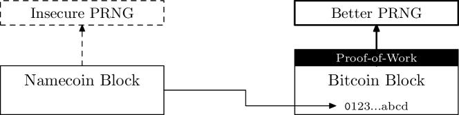
Figure 2: For a merge-mined blockchain like Namecoin, the PoW is not attached to the Namecoin block directly. Instead, a parent block (Bitcoin) is constructed that commits to the Namecoin block’s hash, and the PoW is computed for the parent block. Indirectly, it still depends on the Namecoin block, and thus can secure it. To seed a PRNG in this situation, the parent block (Bitcoin) should be used (bold) instead of the Namecoin block itself (dashed).

Merged mining can be very beneficial for the security of a blockchain. However, its use mandates a tweak to the use of block hashes to seed PRNGs: Since the PoW is not directly part of the block itself, the block hash also does not depend on it. This means that a miner can cheaply generate multiple versions of a block and its block hash, before ever starting the computationally-intensive mining process. Thus, if the randomness of a game were based on the block hash, the miner could simply generate a block he likes first and only then start mining. The opportunity cost of block withholding would be completely removed, making it very easy and cheap to manipulate random numbers.

This problem is straight-forward to fix, though: Instead of basing random numbers off the block hash, they have to depend on some quantity that itself depends on the actual PoW. So by simply using, for instance, the block hash of the parent chain, the same opportunity cost as with a non-merge-mined blockchain is restored. The XAYA blockchain, which can be merge mined with Bitcoin, includes exactly this fix in its rngseed mechanism.

3.3 Hash Commitments

A completely different method for generating provably-fair randomness in a game is based on hash commitments. For the simple case of a game between two players (e.g. one of them could be an online casino), the determination of a random event (e.g. roulette spin) could look like this:

1. Both players choose a secret random number, $N_{1}$ and $N_{2}$. The random event’s outcome will be based on a combination of $N_{1}$ and $N_{2}$, e.g. on the hash $H(N_{1}|N_{2})$ of a concatenation of both.

2. The players share the hashes of their secrets with each other, $H(N_{1})$ and $H(N_{2})$.

3. At this point in time, the secrets and with them the outcome of the random event are fixed. None of the players can change their value anymore without the other noticing, but none can predict the the outcome yet without knowing the other’s secret.

4. After both players have chosen a secret and committed to it, both reveal their preimages $N_{1}$ and $N_{2}$. Now both can verify that the other followed the protocol and both can compute and verify $H(N_{1}|N_{2})$ to determine the random event independently.

Of course, the full protocol for some game based on this approach will likely also include steps where the players sign their messages to each other and/or include them in blockchain transactions, but this is not relevant for the discussion here.

With a protocol like this, both players are guaranteed provably-fair random numbers: As long as the hash function $H$ is cryptographically secure, none of the players can manipulate or predict the outcome.

Hash-commitment schemes are, of course, not new. They have been proposed for cryptographically-secure games long before the invention of Bitcoin, for instance in [18]. In the Bitcoin ecosystem, SatoshiDice [21] was an early gambling platform that utilised hash commitments to provide users with provably-fair betting. Another, more sophisticated example for the use of hash commitments are the “Fate Channels” described by FunFair [17].

But while hash-commitment schemes provide provable security against manipulation, they are unfortunately not applicable in all situations. They are good for games between a well-defined set of players (e.g. just a user and a casino), but they cannot be applied in their basic form for large game worlds with an unspecified set of (currently online) users like Huntercoin. Of course, users might be allowed to contribute data that is integrated into the random-number computation also in these situations. But since it is not known which users can or want to contribute, this has to be optional. Then, however, miners get back the ability to manipulate the randomness at will, since they will be able to censor reveal transactions of users which they do not like; ultimately, the miner of a block will again be the first person to know the outcome, and be able to withhold the block just as discussed above in Subsection 3.1.

4 Betting against Dishonest Miners

As we have seen before in Section 3, none of the existing approaches to random numbers can provide secure randomness for general blockchain games. The usage of block hashes to seed PRNGs works for all kinds of games, but unfortunately suffers from the risk of block withholding. This issue, however, can be fixed by adding an additional feature: Namely by letting users bet “against” miners as first proposed in [9].

Before we describe this idea in more detail, let us take a brief look at a simple and classical game, rock-paper-scissors. It is easy to see (a simple overview can be found in [7]) that the optimal strategy for each player there is to pick each choice randomly with probability $1/3$. As soon as one player deviates from this strategy, she gives an advantage to her opponent who can then exploit the predictability in her strategy. Thus, ideally each player should be as unpredictable as possible, which means randomising the choices as much as possible.

The same can be applied also to randomness based on block hashes: In particular, consider a game where users of a blockchain can bet whether some future block hash will be even or odd. If they bet correctly, they get some money from the miner who created the block in question (their bet minus some house edge). If their bet is wrong, the miner instead wins the amount they wagered.

If a miner produces perfectly randomised block hashes (which is automatically the case as long as he does not engage in block withholding), then this betting game adds some variance to their payout, but overall they win due to the house edge. But as soon as a miner’s blocks have some kind of bias and are no longer fully random, the betting users can get an advantage by exploiting this to win money at the cost of the miner. Thus, the community at large gets an instrument they can apply to punish dishonest miners and hold them accountable. In the next Section 5, we will analyse this game in detail. It will turn out in Theorem 15 that its Nash equilibrium is (under certain conditions) indeed such that the miners will produce blocks that are close to perfectly random instead of withholding them. This holds true even if some miner has a stake in a game on the blockchain as well, and would benefit from manipulating the outcome of random events. Thus, the risk and potential damage of block withholding is greatly reduced by adding the betting game to the blockchain’s rules.

Before continuing, let us clarify the terms we will use in the future for the different roles that participants on the blockchain network have:

Miners

produce blocks as described in Subsection 2.1. Thus they are also ultimately in charge of determining the outcome of random events, which are based on their block hashes. They may also participate in games on the blockchain, and thus have preferences for certain outcomes of those events.

Users

of the blockchain network are, in the context of the following discussion, participants in the betting game described above. They may bet money against miners, particularly if the block distribution produced by the miners is not fully random. They may also participate in games on the blockchain, but this is not relevant for our discussion below.

Players

are simply participants in a blockchain game and they are not mining themselves. The main goal of our proposal is to make sure that players can expect “fair” determination of random events in the games they play.

We assume that all of these actors are rational, and interested only in maximising their profit from within the system. For instance, we assume that no-one is discouraged from an action damaging the blockchain ecosystem (like manipulating randomness) just because it may lower the market value of the underlying cryptocurrency in which they may hold a stake.

4.1 Simplifying Assumptions

To simplify our analysis, let us assume that there is only one miner (who consequently produces all the blocks). Similarly, we consider only one betting user in the system. Of course, this is far from what the reality will be. But if there are multiple agents of each role, then their combined actions will simply amount to a mixed strategy of the game (described in more detail below in Subsection 5.2). For instance, if there is one miner who engages in block withholding and one who does not, then this is equivalent to a single miner who only withholds some blocks. Similarly, if different users on the blockchain bet different amounts (and perhaps on different outcomes), then only the “net bet” is important for the miners.

Furthermore, the mixed system will tend towards the same equilibrium as the game with only one miner and one user: If overall, miners are withholding blocks too often, then it will encourage users (one or multiple) to bet more against them. And then either some of the withholding miners will turn honest (since they are losing money on those bets), or perhaps more honest miners will join (as they can benefit from their house edge). In both cases, the overall fraction of withholding will decrease until the equilibrium is reached, just as a single, rational miner would do. In the same way, overall betting will converge towards the same equilibrium that a single, rational betting user would choose.

Hence, by restricting ourselves to just one miner and a single user (who can and will choose suitable mixed strategies), the overall structure of the game is not changed. (A different way to arrive at the same simplifying assumption is the following: Even if there are multiple miners or users in the system, all of them will have the same incentives and thus behave in the same way, as long as we assume all agents to be rational and interested only in maximising their profits.)

The second simplification we want to make concerns the set of in-game events we consider as targets of miner manipulation and for users to bet on. It is likely that any sufficiently complex blockchain game will need many different random events in its state-transition rules. And while users can then of course bet independently on the different events as they wish, a miner’s decision to publish or withhold a block is “atomic” and cannot be made independently for the different events. But in the end, all that matters to players is that all events relevant to them have the distribution they should have. And if they do not, then users will have an incentive to bet against miners until this is fixed. Individually for each event, this game follows our analysis of Section 5.

4.2 Considerations for a Practical Implementation

It is important to note that it is far from straight-forward to build a practical blockchain that incorporates an implementation of the betting game described above. At least the following issues need to be considered and solved for that:

• User bets will have to be submitted to the network as transactions. They could use some form of hash commitment to hide details about the bet from miners, but miners may still try to censor those transactions (i.e. simply not include them in blocks). Particularly miners who want to manipulate random events may try to do this and block users from holding them accountable. But as long as a user can bet on blocks far enough into the future, it is enough if any (honest) miner confirms her transaction before her bet’s target block.

• Even if honest miners win on average in the betting game (thanks to the house edge), this scheme still increases variance in mining payout and risk for the miners. Thus it may discourage people from mining—although given that the payout expectation is positive, that remains to be seen. Miners on such a blockchain are a mixture between miners of a classical blockchain and casino operators. Since people currently are providing both kinds of services, it seems plausible that there will also be miners on a blockchain based on our proposal.

• It is not trivial how users can actually win money from the miners, especially if the amounts are larger than individual block rewards. To implement this, it will likely be necessary for miners to deposit a large stake of coins in order to be able to produce blocks. Then winnings of users could be taken out of that deposit. This changes the structure of the underlying system significantly (compared to existing PoW blockchains), but does not pose any problems that are impossible to solve. It is important to note here that such a blockchain would still be secured by PoW. Even though miners are required to stake a deposit, this would be very different from the existing concept of proof-of-stake mining.

• For generic blockchains like Ethereum or XAYA, there needs to be some mechanism (e.g. EVM bytecode) to actually define the events that users bet on. For games with their own custom blockchain (e.g. Huntercoin), the developers can instead predefine a list of events that are likely of interest to players in the game.

All in all, defining and building a suitable practical implementation requires additional research and engineering, but is certainly not impossible. This, however, is outside the context of the current paper. Here, we just want to describe the basic idea and show that it is—in theory—able to align the game-theoretic incentives correctly.

5 Game-Theoretic Analysis

Let us now take a detailed look at the game-theoretic incentive structure that the proposed betting game from Section 4 has.

5.1 Basic Setting

Let $(\Omega,\mathcal{F},P)$ be a probability space. (For a general introduction to mathematical probability theory, see, for instance, Chapter 4 of [2].) This probability space models the outcome of mining one block under the assumption that no block withholding is taking place. For a blockchain that uses some $b$-bit hash $h$ based on the block to determine randomness in games, a typical setting will be

$$\Omega=\left\{h\left|\,h\in\mathbb{N}_{0},\;0\leq h<2^{b}\right.\right\},\;\;\mathcal{F}=2^{\Omega},\;\;P\left(A\right)=\frac{\left|A\right|}{2^{b}}.$$

Here, $2^{\Omega}$ denotes the power set of $\Omega$ and $\left|A\right|$ is the number of elements in the finite set $A\subset\Omega$. It is easy to see that this defines, indeed, a (discrete) probability space. The exact nature of the probability space is not relevant for our further analysis, though, and can be left unspecified.

Now, let $D\in\mathcal{F}$ be some fixed event that matters in the blockchain game. In the following, we will analyse the betting game based on this event. For instance, this could be the set of outcomes that lead to some particularly important in-game event in an MMO like Huntercoin, or it could be the set of “winning block hashes” for a casino game like SatoshiDice. Let us denote the probability of $D$ by $p:=P\left(D\right)$.

Next, we consider the reward $R$ that the miner gets for the block—this includes his block reward, but it may also include some winnings (or losses) from in-game events for a miner who also participates in games. Overall, $R$ is a random variable on our probability space. Since our analysis is focused around $D$, let us define the expected miner rewards related to the outcome of this event:

$$R_{d}:=R_{0}+R_{w}:=E\left(R\,|\,D\right),\;\;R_{n}:=R_{0}:=E\left(R\,|\,\Omega\setminus D\right)$$ (1)

Here, $R_{d},R_{n}\in\mathbb{R}$ are the expected rewards of the miner for blocks that trigger $D$ or not, respectively. Without loss of generality, we can assume $R_{d}\geq R_{n}$, i.e. that $D$ is beneficial to the miner. Since $R_{d}=R_{n}$ would make any block withholding and our entire analysis here pointless, we assume furthermore $R_{d}>R_{n}$. As indicated in (1), we can split the expectation values into an unconditional base block reward $R_{0}$ and potential winnings $R_{w}>0$ in the game when $D$ occurs.

5.2 The Betting Game

The process of mining a new block and potentially betting on the outcome of $D$ against the miner (as described in Section 4) can now be seen as a finite game between two players, the miner and the betting user.

5.2.1 Choices for the Miner

For the purpose of this analysis, we assume that before constructing the next block, the miner decides on one of three possible pure strategies:

$H$

The miner can be honest, which means that they will simply broadcast the next block they find, independently of the outcome of $D$.

$W_{d}$

The miner will only broadcast a block where $D$ occurs. He will withhold all blocks that trigger $\Omega\setminus D$ instead. (In other words, the miner withholds to force $D$, not withholds blocks with $D$.)

$W_{n}$

The miner will only broadcast a block where $D$ does not occur. In other words, blocks with $D$ will be withheld and the next published block will trigger $\Omega\setminus D$. Naively, this strategy has no benefit for the miner—but since it is a valid choice, we nevertheless include it in our analysis.

Since we assume that we only have one miner, they are able to force the outcome of $D$ for the next block if they wish (by retrying as often as necessary to find a suitable block). Since creating a block likely incurs a cost to the miner (except perhaps when merge mining), choosing $W_{d}$ or $W_{n}$ as a strategy has an extra cost. This will be reflected in our payoff function (6) below.

Instead of choosing a pure strategy, the miner can of course also pick a mixed strategy that randomises between the three available pure strategies. For this case, let us denote the probabilities of the miner choosing $W_{d}$ and $W_{n}$ by $\omega_{d}$ and $\omega_{n}$, respectively. Then the set of possible strategies for the miner is

$$S_{m}=\left\{(\omega_{d},\omega_{n})\left|\,\omega_{d},\omega_{n}\in[0,1],\;\omega_{d}+\omega_{n}\leq 1\right.\right\}.$$

Clearly, the probability for the miner choosing $H$ is $1-\omega_{d}-\omega_{n}$. By definition of $S_{m}$, this value is also non-negative.

Based on which strategy from $S_{m}$ the miner chooses, the distribution of published blocks may be different from the underlying probability space. In particular, let us define $P_{d}$ and $P_{n}$ to be the probabilities of a mined block triggering $D$ and $\Omega\setminus D$, respectively, under the chosen miner strategy from $S_{m}$. It is easy to see that these quantities are given by

$$P_{d}=\omega_{d}+(1-\omega_{d}-\omega_{n})p,\;\;P_{n}=\omega_{n}+(1-\omega_{d}-\omega_{n})(1-p)=1-P_{d}.$$ (2)

5.2.2 Choices for the Betting User

The user betting against the miner has also three pure strategies available:

$A$

The user can abstain from betting on the outcome of $D$ altogether.

$B_{d}$

The user bets a maximum amount $b_{d}>0$ on $D$ occurring.

$B_{n}$

The user bets a maximum amount $b_{n}>0$ on $\Omega\setminus D$ occurring. As before, this strategy seems not very useful at least from a naive point of view (as also the miner has no incentive to force blocks that do not trigger $D$), but it is a possible strategy to consider.

Just like the miner, the betting user can now also employ a mixed strategy. We denote the probabilities of choosing $B_{d}$ and $B_{n}$ by $\lambda_{d}$ and $\lambda_{n}$, respectively, then the set of possible user strategies is given by

$$S_{u}=\left\{(\lambda_{d},\lambda_{n})\left|\,\lambda_{d},\lambda_{n}\in[0,1],\;\lambda_{d}+\lambda_{n}\leq 1\right.\right\}.$$ (3)

As before, the non-negative probability of choosing $A$ instead is $1-\lambda_{d}-\lambda_{n}$.

Note that opting for a mixed strategy of, say, betting a fixed amount $b_{d}$ with probability $\lambda_{d}$ is (on average) equivalent to always betting a reduced amount $\lambda_{d}b_{d}$. (This can be seen from (5) below.) So instead of defining $S_{u}$ as in (3), we could directly define the user strategy as a pair of non-negative amounts bet on $D$ and $\Omega\setminus D$. But the definition based on a finite amount of available pure strategies and mixed strategies based on them fits better to the typical structure of a game-theoretic analysis. Hence we decided to stick to this form.

5.2.3 Payoff Functions

Let us now take a closer look at the bets that the user can make against the miner. As mentioned above, when playing the pure strategy $B_{d}$, the user bets $b_{d}$. This means that she loses $b_{d}$ if the bet fails ($D$ does not occur). If, on the other hand, $D$ takes place, then she should win an appropriate amount such that the bet is fair (taking the probability $p$ for $D$ into account) and includes a certain house edge $\epsilon>0$. First of all, the winning amount should obviously be proportional to the bet. In other words, let the winning amount be $\beta_{d}b_{d}$ with some factor of proportionality $\beta_{d}>0$. The correct factor can then be determined easily, assuming that we want an honest miner to win on average according to the house edge $\epsilon$:

Lemma 1.

Consider a simple betting game where a user loses the bet $b>0$ with probability $1-p$ and wins $\beta b$ with probability $p>0$. If $\beta$ is chosen as

$$\beta=\frac{1-p}{p+\epsilon},$$

then the expected win is $E\left(W\right)=-\epsilon\beta b$.

Proof.

We can simply check that the expectation value is as claimed:

$$E\left(W\right)=p\beta b-(1-p)b=\frac{(1-p)p-(1-p)(p+\epsilon)}{p+\epsilon}\cdot b=-\frac{(1-p)\epsilon}{p+\epsilon}\cdot b=-\epsilon\beta b$$

∎

Thus, following Lemma 1, we define

$$\beta_{d}=\frac{1-p}{p+\epsilon},\;\;\beta_{n}=\frac{p}{1-p+\epsilon}.$$ (4)

This yields the following expression for the expected payoff of the betting user, based on her strategy $(\lambda_{d},\lambda_{n})\in S_{u}$ and the probabilities $P_{d}$ and $P_{n}$ that depend on the miner’s strategy:

$$E\left(U\right)=\lambda_{d}b_{d}\left(\beta_{d}P_{d}-P_{n}\right)+\lambda_{n}b_{n}\left(\beta_{n}P_{n}-P_{d}\right)$$ (5)

For the miner, let us assume that the expected cost of “forcing” a block that triggers $D$ by withholding all other blocks is given by $C_{d}\geq 0$. Similarly, $C_{n}\geq 0$ shall be the cost of forcing a block where $D$ does not occur. The values of these parameters depend on $p$ and the concrete situation of the blockchain, e.g. the mining difficulty and whether or not the blockchain is merge mined. Overall, the payoff for the miner consists of three parts: First, the expected rewards $R_{d}$ and $R_{n}$ for blocks where $D$ and $\Omega\setminus D$ occur, respectively. Second, the betting game with the user—since this is a zero-sum game, the miner’s payoff is exactly $-U$. And third, the costs for forcing a certain outcome through block withholding. Taking all together, the expected payoff for the miner is

$$E\left(M\right)=P_{d}R_{d}+P_{n}R_{n}-E\left(U\right)-\omega_{d}C_{d}-\omega_{n}C_{n}.$$ (6)

5.3 Strategy for the Betting User

Since we assume that the betting user acts rationally and purely based on maximising her profit, let us now consider what strategy choice in $S_{u}$ maximises $E\left(U\right)$. For this, we assume that some miner strategy from $S_{m}$ is fixed, and that the resulting probabilities $P_{d}$ and $P_{n}=1-P_{d}$ are known to the user. In a real-world setting, these probabilities can simply be determined empirically from an analysis of the last blocks. A first, trivial conclusion is that there exists a (not necessarily unique) optimal user strategy for any given miner strategy (we will fully characterise it later in Corollary 4):

Lemma 2.

For any $P_{d}\in[0,1]$, there exists a user strategy $(\lambda_{d}^{*},\lambda_{n}^{*})\in S_{u}$ that maximises $E\left(U\right)$ over $S_{u}$.

Proof.

This is immediately clear, since $S_{u}$ is compact and $E\left(U\right)$ continuous. (See, for instance, Theorem 2.10 in [16].) ∎

From (5), it is easy to see that the best choice of $(\lambda_{d},\lambda_{n})\in S_{u}$ depends directly on the signs of the two terms $\beta_{d}P_{d}-P_{n}$ and $\beta_{n}P_{n}-P_{d}$. When any one of them is negative, then the corresponding $\lambda$ should be chosen as zero to maximise $E\left(U\right)$. Otherwise, it should be chosen as large as possible. These terms are visualised in Figure 3. If the miner-chosen $P_{d}$ is close to the “natural value” of $p=\numprint{0.4}$, then both terms are negative—this reflects the house edge. But if $P_{d}$ diverges sufficiently from $p$ to either side, then the user’s profits from betting on this divergence exceed the house edge. Clearly, the divergence required to make the terms positive is bigger for a larger house edge (as in Figure 3b). In the limit $\epsilon\to 0^{+}$, the lines intersect at $(p,0)$. Let us also give a more formal and detailed analysis:

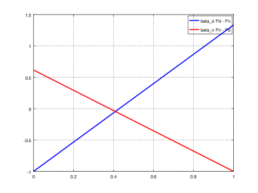
(a) Small house edge, $\epsilon=\numprint{0.05}$

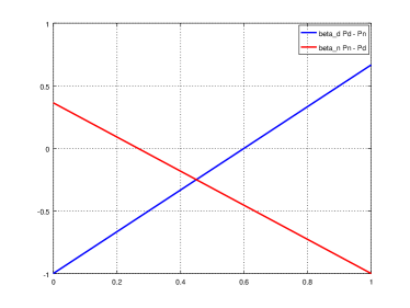
(b) Large house edge, $\epsilon=\numprint{0.5}$

Figure 3: The two terms $\beta_{d}P_{d}-P_{n}$ (blue) and $\beta_{n}P_{n}-P_{d}$ (red) for $p=\numprint{0.4}$. The probability $P_{d}$, which reflects the miner’s strategy, is on the $x$-axis.

Lemma 3.

Let $\epsilon>0$, $p\in(0,1)$ and $P_{d}\in[0,1]$. We set

$$\underline{P_{d}}=\frac{\beta_{n}}{1+\beta_{n}}\text{ and }\overline{P_{d}}=\frac{1}{1+\beta_{d}},$$ (7)

where $\beta_{d}$ and $\beta_{n}$ are defined as in (4). Then

$$0<\underline{P_{d}}<p<\overline{P_{d}}<1.$$ (8)

In the limit for vanishing or very large house edge, some of these inequalities turn into equations:

$$\lim_{\epsilon\to 0^{+}}\underline{P_{d}}=\lim_{\epsilon\to 0^{+}}\overline{P_{d}}=p,\;\;\lim_{\epsilon\to\infty}\underline{P_{d}}=0,\;\;\lim_{\epsilon\to\infty}\overline{P_{d}}=1$$

Furthermore,

$$\mathrm{sgn}\left(\beta_{d}P_{d}-P_{n}\right)=P_{d}-\overline{P_{d}},\;\;\mathrm{sgn}\left(\beta_{n}P_{n}-P_{d}\right)=\underline{P_{d}}-P_{d}.$$ (9)

Here, $\mathrm{sgn}\left(\cdot\right)$ denotes the three-valued sign function (with $\mathrm{sgn}\left(0\right)=0$).

Proof.

Combining (4) with (7), we find that

$$\underline{P_{d}}=\frac{p}{1-p+\epsilon}\cdot\frac{1-p+\epsilon}{1+\epsilon}=\frac{p}{1+\epsilon},\;\;\overline{P_{d}}=\left(\frac{1-p+p+\epsilon}{p+\epsilon}\right)^{-1}=\frac{p+\epsilon}{1+\epsilon}.$$

From these representations, (8) and the stated limits follow easily.

It remains to show (9). For this, note that the following inequalities are equivalent:

$$\beta_{d}P_{d}-P_{n}\geq 0\;\;\Leftrightarrow\;\;\beta_{d}P_{d}\geq 1-P_{d}\;\;\Leftrightarrow\;\;P_{d}\geq\frac{1}{1+\beta_{d}}\;\;\Leftrightarrow\;\;P_{d}-\overline{P_{d}}\geq 0$$

Since the same is true for strict inequalities, the first relation in (9) follows. Similarly,

$$\beta_{n}P_{n}-P_{d}\geq 0\;\;\Leftrightarrow\;\;\beta_{n}(1-P_{d})\geq P_{d}\;\;\Leftrightarrow\;\;\frac{\beta_{n}}{1+\beta_{n}}\geq P_{d}\;\;\Leftrightarrow\;\;\underline{P_{d}}-P_{d}\geq 0.$$

Again, this also holds true for strict inequalities, completing the proof. ∎

The values $\underline{P_{d}}$ and $\overline{P_{d}}$ from Lemma 3 correspond to the points where the red and blue lines in Figure 3, respectively, intersect the $x$-axis. They determine the optimal user strategy:

Corollary 4.

The set $S_{u}^{*}\subset S_{u}$ of user strategies that maximise $E\left(U\right)$ is given as follows:

• If $P_{d}<\underline{P_{d}}$, then the user can make a profit by betting on $\Omega\setminus D$. Consequently, the unique optimal strategy is to choose $\lambda_{d}=0$ and $\lambda_{n}=1$, i.e. $S_{u}^{*}=\left\{(0,1)\right\}$.

• If $\underline{P_{d}}<P_{d}<\overline{P_{d}}$, then the user should not bet at all. In this range, the distribution of blocks produced by the miner is so close to the “true” distribution (determined by $p$) that the house edge is larger than any potential winnings. In this case, $S_{u}^{*}=\left\{(0,0)\right\}$.

• If $\overline{P_{d}}<P_{d}$, then the user can make a profit by betting on $D$. The user should choose $\lambda_{d}=1$ and $\lambda_{n}=0$ to maximise $E\left(U\right)$, i.e. $S_{u}^{*}=\left\{(1,0)\right\}$.

• For the two “intermediate” cases $P_{d}=\underline{P_{d}}$ and $P_{d}=\overline{P_{d}}$, the user can choose to bet or not, since the expected winnings from the skewed distribution will exactly compensate for the house edge. Thus all strategies with $\lambda_{d}=0$ and $\lambda_{n}\in[0,1]$ are optimal for $P_{d}=\underline{P_{d}}$, i.e. $S_{u}^{*}=\left\{0\right\}\times[0,1]$. Similarly, $S_{u}^{*}=[0,1]\times\left\{0\right\}$ for $P_{d}=\overline{P_{d}}$.

Proof.

This follows from (5) and Lemma 3. ∎

Note that (8) implies that it is never optimal for the user to bet on both outcomes at the same time (i.e. $\lambda_{d}>0$ and $\lambda_{n}>0$). “Hedging the bet” like this always means that she loses unnecessarily much to the house edge.

5.4 Strategy for the Miner

Also the miner is trying to optimise his profit, i.e. to maximise $E\left(M\right)$ by choosing $(\omega_{d},\omega_{n})\in S_{m}$ in the right way for a given user strategy in $S_{u}$. Noting that $P_{n}=1-P_{d}$ and using $R_{0}$ and $R_{w}$ to express the block rewards, we can rewrite (6) to:

$$E\left(M\right)=P_{d}(R_{0}+R_{w})+(1-P_{d})R_{0}-E\left(U\right)-\omega_{d}C_{d}-\omega_{n}C_{n}=R_{0}+P_{d}R_{w}-E\left(U\right)-\omega_{d}C_{d}-\omega_{n}C_{n}$$ (10)

Since $R_{0}$ is just a constant offset, it is clear that we can, without loss of generality, assume $R_{0}=0$ and use the simplified form (10) for analysing the maximum. (The base block reward $R_{0}$ is of course important to incentivise miners in the first place. But for our analysis here, we assume that there is a miner on the blockchain anyway. For determining his strategy with respect to block withholding, the value of $R_{0}$ does not matter.)

A first observation we can make about (10) is the following: The first part of the expression depends only on $P_{d}$, but not directly on $\omega_{d}$ or $\omega_{n}$. Only the last two terms (expressing the cost for withholding blocks) are given based on $\omega_{d}$ and $\omega_{n}$ directly, and they are always “bad” for maximising the profit. Furthermore, the miner can achieve an arbitrary value of $P_{d}\in[0,1]$ with at least one of the two withholding probabilities set to zero:

Lemma 5.

Let a desired $P_{d}\in[0,1]$ be given arbitrarily. This value of $P_{d}$ can be achieved according to (2) with a miner strategy $\omega^{*}=(\omega_{d}^{*},\omega_{n}^{*})\in S_{m}$, where $\omega_{d}^{*}=0$ if $P_{d}\leq p$ and $\omega_{n}^{*}=0$ if $P_{d}\geq p$.

Furthermore, any other strategy $(\omega_{d},\omega_{n})\in S_{m}$ that yields $P_{d}$ satisfies $\omega_{d}>\omega_{d}^{*}$ and $\omega_{n}>\omega_{n}^{*}$.

Proof.

Setting $\omega_{d}^{*}=0$ and solving (2) for $\omega_{n}^{*}$ yields $\omega_{n}^{*}=1-P_{d}/p$. For $P_{d}\leq p$, we have $\omega_{n}^{*}\in[0,1]$, so that $\omega^{*}\in S_{m}$. Similarly, $\omega_{n}^{*}=0$ and $\omega_{d}^{*}=(P_{d}-p)/(1-p)$ also yield a valid strategy if $P_{d}\geq p$. In the special situation of $P_{d}=p$, both cases result in $\omega_{d}^{*}=\omega_{n}^{*}=0$.

Now let $\omega=(\omega_{d},\omega_{n})\in S_{m}$ be another strategy that results in the given value of $P_{d}$. For $P_{d}\leq p$, clearly $\omega_{d}\geq\omega_{d}^{*}=0$. Also, solving (2) for $\omega_{n}$, we get

$$\omega_{n}=1-\frac{P_{d}}{p}+\frac{1-p}{p}\cdot\omega_{d}=\omega_{n}^{*}+\frac{1-p}{p}\cdot\omega_{d}\geq\omega_{n}^{*}.$$

If $\omega_{d}=\omega_{d}^{*}=0$ would be the case, then also $\omega_{n}=\omega_{n}^{*}$ follows. This contradicts the assumption that $\omega^{*}\neq\omega$. Thus $\omega_{d}>\omega_{d}^{*}$ and $\omega_{n}>\omega_{n}^{*}$ must in fact be true.

For $P_{d}\geq p$, a similar argument shows $\omega_{n}>\omega_{n}^{*}=0$ and

$$\omega_{d}=\omega_{d}^{*}+\frac{p}{1-p}\cdot\omega_{n}>\omega_{d}^{*}.$$

∎

Thus, we can conclude that the optimal miner strategy will be found in the set

$$S_{m}^{0}=\left([0,1]\times\left\{0\right\}\right)\cup\left(\left\{0\right\}\times[0,1]\right)\subset S_{m},$$

where at least one withholding probability is zero:

Corollary 6.

$E\left(M\right)$ has a maximum over the set $S_{m}$. This maximum can be achieved even with $\omega^{*}\in S_{m}^{0}$. If $C_{d},C_{n}>0$ are strictly positive, then only strategies from $S_{m}^{0}$ can maximise $E\left(M\right)$.

Proof.

Since $S_{m}$ is compact and $E\left(M\right)$ continuous, it is clear that there exists a maximising strategy $\omega\in S_{m}$. This strategy has a corresponding optimal value $P_{d}(\omega)\in[0,1]$. Thus, Lemma 5 implies that there exists $\omega^{*}\in S_{m}^{0}$ with $P_{d}(\omega^{*})=P_{d}(\omega)$. And since $\omega\geq\omega^{*}$ component-wise according to the lemma, it follows from $C_{d},C_{n}\geq 0$ and (10) that $E\left(M(\omega)\right)\leq E\left(M(\omega^{*})\right)$. If $C_{d},C_{n}>0$, then $\omega=\omega^{*}$ must be the case, since otherwise $E\left(M(\omega)\right)<E\left(M(\omega^{*})\right)$ and that contradicts our assumption of $\omega$ being a maximum. ∎

Note that $E\left(M\right)$ is an affine function with respect to $\omega_{d}$ and $\omega_{n}$. The coefficients depend on the user strategy $(\lambda_{d},\lambda_{n})\in S_{u}$ and the parameters like $R_{w}$ or $C_{d}$. Thus, one can in theory easily compute where exactly on $S_{m}^{0}$ the optimal miner strategy lies once those coefficients are fixed. In full generality, however, this is a bit messy and not very enlightening. In the following we will instead consider special cases that yield more qualitative conclusions as well as results relevant for determining the Nash equilibrium of the betting game later in Subsection 5.5.

The first property that we can deduce is quite intuitive: If the user bets on $\Omega\setminus D$, then the miner should certainly not try to force this outcome. Not only will he lose money to the user, he will also have costs for doing so and result in lower block rewards than not withholding any blocks (or forcing $D$).

Lemma 7.

Let the user strategy satisfy $\lambda_{d}=0$ and assume that $\omega^{*}=(\omega_{d}^{*},\omega_{n}^{*})\in S_{m}^{0}$ maximises $E\left(M\right)$. Then necessarily $\omega_{n}^{*}=0$.

Proof.

Assume to the contrary that $\omega_{n}^{*}>0$. Since $\omega^{*}\in S_{m}^{0}$, this implies $\omega_{d}^{*}=0$. Hence, $P_{d}(\omega^{*})<p=P_{d}(\omega_{0})$, where $\omega_{0}=(0,0)\in S_{m}^{0}$ corresponds to the miner strategy $H$ of being fully honest and not withholding any blocks.

For $\lambda_{d}=0$ and $\omega_{d}=0$, the miner payoff (10) simplifies to

$$E\left(M\right)=P_{d}R_{w}-E\left(U\right)-\omega_{n}C_{n}=P_{d}R_{w}-\lambda_{n}b_{n}(\beta_{n}P_{n}-P_{d})-\omega_{n}C_{n}.$$

The first two terms are strictly increasing in $P_{d}$ and the last is decreasing in $\omega_{n}$. Hence, it follows that $E\left(M(\omega^{*})\right)<E\left(M(\omega_{0})\right)$, contradicting optimality of $\omega^{*}$. ∎

Of course, since $D$ is beneficial to the miner, one may expect the miner to produce blocks that trigger $D$ more often rather than less often, i.e. $P_{d}\geq p$. Hence, the natural strategy for the betting user (according Corollary 4) likely has $\lambda_{n}=0$ rather than $\lambda_{d}=0$. In this case, the optimal miner strategy depends on the exact relation between the benefit $R_{w}$ that $D$ has for the miner, the cost $C_{d}$ for forcing $D$ and the user’s bet $\lambda_{d}$. In particular:

Proposition 8.

Let $\lambda_{n}=0$, $C_{d},C_{n}>0$ and define

$$\Lambda:=\lambda_{d}b_{d}(\beta_{d}+1),\;\;\underline{\Lambda}:=R_{w}-\frac{C_{d}}{1-p}<R_{w}+\frac{C_{n}}{p}=:\overline{\Lambda}.$$ (11)

Then the set $S_{m}^{*}\subset S_{m}$ of miner strategies that maximise $E\left(M\right)$ is given as follows:

• If $\Lambda<\underline{\Lambda}$, then the rewards of blocks with $D$ outweigh the costs of forcing them. The miner should choose $\omega_{d}=1$ and $\omega_{n}=0$, i.e. $S_{m}^{*}=\left\{(1,0)\right\}$.

• If $\underline{\Lambda}<\Lambda<\overline{\Lambda}$, then the user bets roughly equal the rewards $R_{w}$ that the miner can achieve with blocks that trigger $D$. The costs for forcing either $D$ or $\Omega\setminus D$ outweigh any benefits, so the optimal miner strategy is to be honest with $S_{m}^{*}=\left\{(0,0)\right\}$.

• If $\overline{\Lambda}<\Lambda$, then user bets on $D$ are so high that the miner can actually benefit the most by forcing blocks that trigger $\Omega\setminus D$. He should choose $\omega_{d}=0$ and $\omega_{n}=1$, i.e. $S_{m}^{*}=\left\{(0,1)\right\}$.

• For the intermediate cases with equality, the miner can choose any mixed strategy between the two equal choices. In other words, for $\Lambda=\underline{\Lambda}$, $S_{m}^{*}=[0,1]\times\left\{0\right\}$. For $\Lambda=\overline{\Lambda}$, the optimal strategies are given by $S_{m}^{*}=\left\{0\right\}\times[0,1]$.

Proof.

For $\lambda_{n}=0$, we can rewrite $E\left(M\right)$ from (10) as

$$E\left(M\right)=X_{d}\omega_{d}+X_{n}\omega_{n}+X_{0},$$

where the coefficients are given by

$$\begin{split}X_{d}&=R_{w}(1-p)-C_{d}-\Lambda(1-p),\\ X_{n}&=\Lambda p-R_{w}p-C_{n},\\ X_{0}&=R_{w}p+\lambda_{d}b_{d}(1-p(\beta_{d}+1)).\end{split}$$

From these values, it is easy to see that $\mathrm{sgn}\left(X_{d}\right)=\mathrm{sgn}\left(\underline{\Lambda}-\Lambda\right)$ and $\mathrm{sgn}\left(X_{n}\right)=\mathrm{sgn}\left(\Lambda-\overline{\Lambda}\right)$. Since $\underline{\Lambda}<\overline{\Lambda}$, at most one of the two can be positive (this matches the result of Corollary 6). The optimal miner strategies $S_{m}^{*}$ as stated follow easily. ∎

Let us conclude this subsection with two remarks about Proposition 8: First, note that (4) implies

$$X_{0}=R_{w}p+\epsilon\beta_{d}\cdot\lambda_{d}b_{d}>0.$$

Thus, the miner payoff for being honest is always positive and corresponds to what one expects from Lemma 1. Second, it can of course be the case that not all of the options in Proposition 8 are actually applicable. For instance, if $R_{w}$ is very small compared to the cost $C_{d}$, then $\underline{\Lambda}<0$ can be the case. This means that $W_{d}$ (forcing blocks that trigger $D$) is never a good choice for the miner, even if $\lambda_{d}=0$.

5.5 Nash Equilibria of the Betting Game

After having analysed the optimal strategies for both the miner and betting user previously, we can now consider them together. To analyse the general structure of the betting game, we employ the widely-used concept of Nash equilibria [11]. For a more extensive introduction to this concept, see Chapter 2 of [12]. Roughly speaking, a Nash equilibrium occurs in a game if every player uses the optimal strategy assuming that all other players stick to their chosen strategy. In other words, when all players choose a strategy from such an equilibrium point, then none of them has an incentive to unilaterally switch to a different strategy. In the context of our the betting game, this means (compare Definition 14.1 in [12]):

Definition 9.

A pair of strategies $(\omega,\lambda)\in S_{m}\times S_{u}$ is a Nash equilibrium if $\omega$ maximises $E\left(M(\lambda)\right)$ over $S_{m}$ and $\lambda$ maximises $E\left(U(\omega)\right)$ over $S_{u}$.

It is not hard to see that Proposition 20.3 of [12] applies in our situation, showing that a Nash equilibrium exists. In the remainder of this subsection, however, we will characterise the Nash equilibria of our betting game more thoroughly. For this, we will assume $C_{d},C_{n}>0$. This acts as a kind of regularisation (see Corollary 6), and will reduce the number of special cases we have to consider.

The first result that we can derive is that the “negative” strategies $W_{n}$ and $B_{n}$, as well as mixed strategies involving them, can never be part of a Nash equilibrium. This already simplifies our analysis of the equilibria quite a lot.

Lemma 10.

Let $(\omega,\lambda)\in S_{m}\times S_{u}$ be a Nash equilibrium. Then necessarily $\omega_{n}=0$ and $\lambda_{n}=0$.

Proof.

Assume to the contrary that $\omega_{n}>0$. According to Corollary 6, this implies $\omega_{d}=0$. Hence, $P_{d}<p$ must be the case (i.e. the miner forces $\Omega\setminus D$ to occur more often than it would naturally). In this situation, Corollary 4 implies $\lambda_{d}=0$ for an optimal user strategy. But then Lemma 7 implies $\omega_{n}=0$, which is a contradiction.

Now assume $\lambda_{n}>0$ instead. Since $\lambda$ is a maximising strategy for the user, this means per Corollary 4 that $P_{d}<p$ must be the case. This, in turn, is only possible if $\omega_{n}>0$. But then we arrive at a contradiction as in the first part of the proof. ∎

As our next step, we consider a first special case: If the reward $R_{w}$ for blocks that trigger $D$ is so small that the cost $C_{d}$ for forcing them outweighs any benefits for the miner, then the equilibrium point of the betting game is with the miner acting honestly and the user not betting at all. In this case, random numbers will be fair simply because the miner has no sufficient incentive to fiddle with them. (Just as they would be fair in this situation without a betting game.)

Proposition 11.

Assume that $R_{w}<C_{d}/(1-p)$. Then the unique Nash equilibrium of the betting game is $\omega_{d}=\omega_{n}=\lambda_{d}=\lambda_{n}=0$, i.e. the pure strategy $(H,A)$.

Proof.

Note that our assumption together with (11) implies $\underline{\Lambda}<0$, so that $\underline{\Lambda}<\Lambda$ is always the case for Proposition 8. Let $(\omega,\lambda)\in S_{m}\times S_{u}$ be a Nash equilibrium. Then Lemma 10 implies $\omega_{n}=\lambda_{n}=0$. Thus we can conclude from Proposition 8 that $\omega_{d}=0$ must be the case as well. Consequently $P_{d}=p$, so that $\lambda_{d}=0$ follows from Corollary 4.

It remains to verify that $(H,A)$ actually is a Nash equilibrium. (This follows also from the known existence of an equilibrium, but it is not hard to check directly.) For $\omega_{d}=\omega_{n}=0$, $P_{d}=p$. Thus $\lambda=(0,0)$ is indeed an optimal strategy for the user according to Corollary 4. The other way round, for $\lambda_{d}=\lambda_{n}=0$ and $\underline{\Lambda}<\Lambda$, the case $\underline{\Lambda}<\Lambda=0<\overline{\Lambda}$ is active in Proposition 8, implying that $\omega=(0,0)$ is the optimal miner strategy. This completes the proof. ∎

The second special case is where $R_{w}$ is large enough to incentivise block withholding, but where also the maximum bet $b_{d}$ is so small that even if the user bets that maximum, then the miner still benefits by forcing all blocks to trigger $D$. In the extreme case $b_{d}=0$, this corresponds to the typical situation where block hashes are used for random numbers but no betting game is there at all.

Proposition 12.

Assume $0<b_{d}(\beta_{d}+1)<R_{w}-C_{d}/(1-p)$. Then the unique Nash equilibrium of the betting game is $\omega_{n}=\lambda_{n}=0$ and $\omega_{d}=\lambda_{d}=1$, i.e. the pure strategy $(W_{d},B_{d})$.

Proof.

As before, let $(\omega,\lambda)\in S_{m}\times S_{u}$ be a Nash equilibrium and recall that $\omega_{n}=\lambda_{n}=0$ must be the case according to Lemma 10. In the situation we consider, $\Lambda<\underline{\Lambda}$ is always the case (for all possible $\lambda_{d}\in[0,1]$). Thus Proposition 8 implies $\omega_{d}=1$. Then $P_{d}=1$, so that the optimal user strategy is $\lambda_{d}=1$ according to Corollary 4. Using the same results, we can also easily verify that the pair of pure strategies $(W_{d},B_{d})$ actually is a Nash equilibrium. ∎

We can now also consider the case between the two previous extremes. In that situation, the equilibrium is given by a mixed strategy:

Proposition 13.

Let $0<R_{w}-C_{d}/(1-p)<b_{d}(\beta_{d}+1)$ be the case. Then the betting game has a unique Nash equilibrium at a mixed strategy between $(H,A)$ and $(W_{d},B_{d})$. In particular, $\omega_{n}=\lambda_{n}=0$ and

$$\omega_{d}=\frac{\epsilon}{1+\epsilon},\;\;\lambda_{d}=\frac{1}{b_{d}(\beta_{d}+1)}\left(R_{w}-\frac{C_{d}}{1-p}\right).$$ (12)

Proof.

Assume that $(\omega,\lambda)\in S_{m}\times S_{u}$ is a Nash equilibrium. Then Lemma 10 implies $\omega_{n}=\lambda_{n}=0$. Consequently also $P_{d}\geq p$. Next, consider (7) and note that $P_{d}=\overline{P_{d}}$ if and only if $\omega_{d}$ is chosen as in (12). Assume for a moment that $\omega_{d}$ is larger, which means $P_{d}>\overline{P_{d}}$. Then Corollary 4 implies that $\lambda_{d}=1$ must be the case for an equilibrium point as per Definition 9. Hence $\underline{\Lambda}<\Lambda$ is the case in (11) for the situation we consider. But then $\omega_{d}=0$ according to Proposition 8, which contradicts $P_{d}>\overline{P_{d}}>p$. So consider the situation that $\omega_{d}$ is smaller, i.e. $P_{d}<\overline{P_{d}}$. Then Corollary 4 implies $\lambda_{d}=0$, so that $\Lambda=0<\underline{\Lambda}$ in Proposition 8. Thus $\omega_{d}=1$ must be the case for an optimal miner strategy, but that contradicts $P_{d}<\overline{P_{d}}$ as it would imply $P_{d}=1$. Hence we have shown $P_{d}=\overline{P_{d}}$, which means that $\omega_{d}$ must be as in (12).

Similarly, note that $\lambda_{d}$ matches (12) if and only if $\Lambda=\underline{\Lambda}$ in (11). Assume that $\Lambda<\underline{\Lambda}$ would be the case. Then Proposition 8 implies $\omega_{d}=1$. For $\underline{\Lambda}<\Lambda$, $\omega_{d}=0$ follows. Both contradict the already shown form of $\omega_{d}$ according to (12), though, so that $\Lambda=\underline{\Lambda}$ must be the case. Thus we have shown that the Nash equilibrium $(\omega,\lambda)$ necessarily has the form claimed in (12).

It remains to show that (12) is also sufficient for $(\omega,\lambda)$ being a Nash equilibrium. For this, note first that $\omega_{d}$ and $\lambda_{d}$ from (12) are both valid strategy choices in $(0,1)$. As noted already above, they furthermore imply exactly $P_{d}=\overline{P_{d}}$ and $\Lambda=\underline{\Lambda}$. Thus, it follows from Corollary 4 that $\lambda_{d}$ is optimal for $\omega_{d}$ (in fact, any $\lambda_{d}\in[0,1]$ would be optimal). Similarly, Proposition 8 implies that also $\omega_{d}$ (and in fact any $\omega_{d}\in[0,1]$) is optimal for $\lambda_{d}$. Thus, $(\omega,\lambda)$ is a Nash equilibrium according to Definition 9. ∎

The equilibrium point from (12) can be interpreted as follows: Due to the positive benefit $R_{w}$ that the miner has for blocks that trigger $D$, he has an incentive to slightly prefer those blocks instead of producing fully random outcomes. But since the user is able to bet against the miner, she will do so to make a profit from the knowledge that $D$ blocks are more frequent than they should be. In the end, the miner skews the distribution just so much that the losses to the betting user equal the benefits from $R_{w}$. For the user, on the other hand, the winnings thanks to the skewed distribution are just equal to the miner’s house edge. In this situation, the miner benefits compared to a situation without any block withholding and without any bets, and the user enjoys “free betting”. Furthermore, the situation is even beneficial for miners that are honest and not interested in block withholding in the first place: They benefit from a non-zero amount of bets being made; the profit they make due to the house edge is exactly equal to the benefit they could get from manipulating the randomness and exploiting $R_{w}$ instead.

Finally, it remains to consider the situations exactly on the border between the previous three cases. For them, it will turn out that there are multiple equilibrium points. That is because the user strategy will be on the boundary of its domain ($\lambda_{d}\in\left\{0,1\right\}$). With active constraints, the user’s strategy choice is less flexible, so that multiple miner strategies can be optimal at the same time.

Proposition 14.

Let us denote the set of Nash equilibria of the betting game by $\Sigma^{*}\subset S_{m}\times S_{u}$.

If $R_{w}=C_{d}/(1-p)$, then

$$\Sigma^{*}=\left\{(\omega_{d},0,\lambda_{d},0)\left|\,\lambda_{d}=0,\;\;0\leq\omega_{d}\leq\frac{\epsilon}{1+\epsilon}\right.\right\}.$$ (13)

For $0<b_{d}(\beta_{d}+1)=R_{w}-C_{d}/(1-p)$, we have

$$\Sigma^{*}=\left\{(\omega_{d},0,\lambda_{d},0)\left|\,\lambda_{d}=1,\;\;\frac{\epsilon}{1+\epsilon}\leq\omega_{d}\leq 1\right.\right\}.$$ (14)

Proof.

Let us first consider the case $R_{w}=C_{d}/(1-p)$, and let $(\omega,\lambda)\in S_{m}\times S_{u}$ be a Nash equilibrium. Then clearly $\omega_{n}=\lambda_{n}=0$ according to Lemma 10. Furthermore, in this case we have $\underline{\Lambda}=0$. If $\lambda_{d}>0$, then also $\Lambda>0$ as well. Hence $\underline{\Lambda}<\Lambda$ implies $\omega_{d}=0$ through Proposition 8. But then $P_{d}=p$ and thus $\lambda_{d}=0$ according to Corollary 4. This is a contradiction, so that $\lambda_{d}=0$ must necessarily be true. But $\lambda_{d}=0$ is only an optimal strategy according to Corollary 4 if $P_{d}\leq\overline{P_{d}}$. This, in turn, is equivalent to $\omega_{d}\leq\epsilon/(1+\epsilon)$. Hence, $(\omega,\lambda)$ is indeed in the right-hand side of (13).

Next, let $(\omega,\lambda)$ be in the right-hand side of (13). We have to show that it is actually a Nash equilibrium. Since $\lambda_{d}=0$, we know that $\Lambda=\underline{\Lambda}=0$. Thus, any value for $\omega_{d}$ corresponds to an optimal miner strategy as per Proposition 8. For $\omega_{d}\leq\epsilon/(1+\epsilon)$, we know that $P_{d}\leq\overline{P_{d}}$ as before. Hence, $\lambda_{d}=0$ is an optimal strategy for the user according to Corollary 4.

The second case to consider is $b_{d}(\beta_{d}+1)=R_{w}-C_{d}/(1-p)$. Let $(\omega,\lambda)$ be a Nash equilibrium. If $\lambda_{d}<1$, then $\Lambda<\underline{\Lambda}$. Hence $\omega_{d}=1$ must be the case for an optimal miner strategy according to Proposition 8. But then $P_{d}=1$, so that $\lambda_{d}<1$ cannot be optimal per Corollary 4. Hence, $\lambda_{d}=1$ must be the case. This, however, is only optimal if $P_{d}\geq\overline{P_{d}}$, which in turn is equivalent to $\omega_{d}\geq\epsilon/(1+\epsilon)$. Thus, $(\omega,\lambda)$ must be in the right-hand side of (14).

Finally, consider any $(\omega,\lambda)$ in the right-hand side of (14). From $\lambda_{d}=1$, it follows that $\Lambda=\underline{\Lambda}$. Hence, any $\omega_{d}$ yields an optimal miner strategy as per Proposition 8. Also, the lower bound that we have on $\omega_{d}$ implies $P_{d}\geq\overline{P_{d}}$, so that $\lambda_{d}=1$ is actually optimal for the user according to Corollary 4. Thus, $(\omega,\lambda)\in\Sigma^{*}$. This completes the proof. ∎

With the previous results, we have now fully characterised the Nash equilibria of our betting game in various situations. Note that the miner withholding $\omega_{d}$ is always bounded away from one in a Nash equilibrium, except if $b_{d}$ is too small. But since $b_{d}$ is just a parameter of the system, it can be chosen large enough to enable a meaningful betting game against miner withholding. Hence, we can conclude that the betting game is indeed efficient at ensuring that the randomness in our blockchain game is close to perfectly fair:

Theorem 15.

Assume $C_{d},C_{n}>0$ and that $b_{d}$ is chosen large enough, i.e. such that

$$b_{d}(\beta_{d}+1)>R_{w}-\frac{C_{d}}{1-p}.$$ (15)

Then for any Nash equilibrium of the betting game,

$$0\leq\omega_{d}\leq\frac{\epsilon}{1+\epsilon}\text{ and }p\leq P_{d}\leq\frac{p+\epsilon}{1+\epsilon}.$$ (16)

In particular, $P_{d}$ will be arbitrarily close to $p$ if the house edge $\epsilon$ is chosen small enough.

Proof.

For the case of (15), one of Proposition 11, Proposition 13 or the first part of Proposition 14 applies. All of them yield $\omega_{n}=0$ and $\omega_{d}$ as in (16). The bound on $P_{d}$ from (16) follows then immediately by (2). Finally, it is also easy to see that $P_{d}\to p$ from above as $\epsilon\to 0^{+}$. ∎

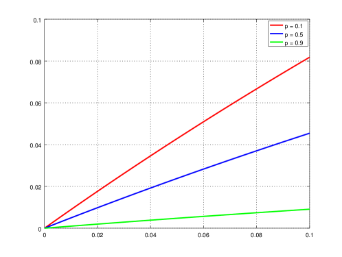
Figure 4: The deviation of $P_{d}$ from $p$ in the Nash equilibrium according to Theorem 15. The house edge $\epsilon$ is on the $x$-axis. The $y$-axis shows the upper bound for $P_{d}-p=\left|P_{d}-p\right|$.

Figure 4 shows numerical values for the bounds on the deviation of $P_{d}$ from the true $p$ according to (16). The three lines correspond to different values of $p$. It can be seen that the betting game is most efficient in reducing the miner-created skew in the distribution of $D$ if $D$ is likely to occur, and least efficient for events that occur rarely. This can be explained by the fact that block withholding has the most effect for the miner if the event would naturally occur only infrequently. But it can also be seen that even a huge house edge of 10% only makes a 50-50 event occur 55% instead of 50% of the time. For a more competitive house edge of 1%, this deviation drops to just slightly more than 0.5%. For most random events in games, this is barely noticeable—and definitely a lot better than the situation without betting, where the miner would (if only interested in profit) force the event to occur 100% of the time instead.

6 Conclusion

The current state of the art for randomness in blockchain games relies on one of two methods, using block hashes to seed PRNGs or basing random events on hash commitments from the players. We have discussed that both approaches have drawbacks under certain circumstances and for certain types of games. However, randomness from block hashes can be improved by introducing a special betting game. Using game theory, we have shown that this game leads to Nash equilibria where the observed distribution for a certain random event matches the expected, fair distribution quite well. In other words, introducing our betting game changes the incentive structure for miners in such a way that they will no longer manipulate the randomness completely. Instead, the game will be much fairer for every player.

We believe that this is a very interesting result. It shows that it is possible to use game-theoretic incentives to produce fair “randomness” in a deterministic context like a blockchain. Our analysis from Section 5 has proven the general idea to work. However, research in this topic is of course not complete yet. In our opinion, there are two main directions where further work would be very interesting and useful:

First, we made a lot of assumptions for the analysis here (see Subsection 4.1). Further work is required to remove those and check whether our results still hold in more general contexts. Particularly interesting would be an analysis with more agents than just one miner and one user. Also important is work on a situation where there is more than one event. For the latter, betting could still be done on individual events. But the miner strategy would consist of a full probability distribution on $\Omega$, likely deviating from the natural distribution given by $P$. A full analysis of this situation will require different mathematics from the current paper and would be heavier in topics like functional analysis and measure theory. Hence, it should be done in a separate paper. We believe that this would not change the fundamental results, though. It is conceivable that there would still be one particular event or outcome that maximises the miner’s benefit $R_{w}$, so that the miner strategy would then still be focused on withholding blocks just for this particular event. Finally, a third assumption we made is that the betting user actually knows $R_{w}$. This is not the case (at least not exactly) for a real-world implementation, since it depends heavily on how the miner is involved in the game himself (and if at all). So the analysis could be adapted to be more probabilistic in nature, e.g. using Bayesian game theory. In the end, however, only the value of $P_{d}$ matters for the user strategy—and that one can be observed empirically. So at least if the system still tends towards some kind of equilibrium, this will yield the same results as our current analysis.

Second, it remains to implement and test our proposal in a real-world system. Only that can show whether or not agents will really behave as analysed and thus produce good randomness. We have already listed the main issues to overcome for such an implementation above in Subsection 4.2. For such a test, it is interesting to note that random numbers can in theory be separated from mining: Instead of basing them off a block hash and putting miners in charge, there could be a separate class of agents that are just responsible for producing random numbers. That would, of course, reduce the costs $C_{d}$ and $C_{n}$ drastically and thus make the system even more susceptible to manipulation. But the betting game may still be able to rectify the incentives even in such a system. The advantage of an implementation like that is that it could be done on top of an existing blockchain, e.g. in an Ethereum smart contract or a game on the XAYA platform. There would be no need to build a blockchain from scratch. Getting real-world results for how the betting game behaves in such a system would be very interesting.

References

- [1] Andreas M. Antonopoulos. Mastering Bitcoin: Unlocking Digital Cryptocurrencies. O’Reilly Media, 2014.
- [2] Robert B. Ash and Catherine Doléans-Dade. Probability and Measure Theory. Harcourt Academic Press, second edition, 2000.
- [3] Adam Back. A partial hash collision based postage scheme. http://www.hashcash.org/papers/announce.txt, 1997.
- [4] Steven Buchko. What is Merged Mining? A Potential Solution to 51% Attacks. Coin Central, https://coincentral.com/merged-mining/, 2018.
- [5] Vitalik Buterin. A Next-Generation Smart Contract and Decentralized Application Platform. https://github.com/ethereum/wiki/wiki/White-Paper, 2013.
- [6] Evelyn Cheng. Meet CryptoKitties, the $100,000 digital beanie babies epitomizing the cryptocurrency mania. CNBC, https://www.cnbc.com/2017/12/06/meet-cryptokitties-the-new-digital-beanie-babies-selling-for-100k.html, 2017.
- [7] Patrick Honner. Why Winning in Rock-Paper-Scissors (and in Life) Isn’t Everything. Quanta Magazine, https://www.quantamagazine.org/the-game-theory-math-behind-rock-paper-scissors-20180402/, 2018.
- [8] Daniel Kraft. Games on the Blockchain. https://github.com/xaya/Specs/blob/master/games.md, 2018.
- [9] Daniel Kraft. Random numbers in a blockchain. Bitcointalk, https://bitcointalk.org/index.php?topic=5072435.0, 2018.
- [10] Satoshi Nakamoto. Bitcoin: A Peer-to-Peer Electronic Cash System. https://bitcoin.org/bitcoin.pdf, 2008.
- [11] John F. Nash. Equilibrium Points in -Person Games. Proceedings of the National Academy of Sciences, 36(1):48–49, 1950.
- [12] Martin J. Osborne and Ariel Rubinstein. A Course in Game Theory. MIT Press, 1994.
- [13] PhantomPhreak. [ANN][XCP] Counterparty - Pioneering Peer-to-Peer Finance - Official Thread. Bitcointalk, https://bitcointalk.org/index.php?topic=395761.0, 2014.
- [14] Piotr J. Piasecki. Gaming Self-Contained Provably Fair Smart Contract Casinos. Ledger, 1:99–110, 2016. DOI 10.5195/LEDGER.2016.29.
- [15] Ruben Alexander. HunterCoin: The Massive Multiplayer Online Cryptocoin Game (MMOCG). Bitcoin Magazine, https://bitcoinmagazine.com/articles/huntercoin-the-massive-multiplayer-online-cryptocoin-game-mmocg-1409336751/, 2014.
- [16] Walter Rudin. Real and Complex Analysis. McGraw-Hill Book Company, third edition, 1987.
- [17] Jez San. Randomness is a big deal. https://funfair.io/randomness-is-a-big-deal/, 2017.
- [18] Adi Shamir, Ronald L. Rivest, and Leonard M. Adleman. Mental Poker. In David A. Klarner, editor, The Mathematical Gardner, pages 37–43. Prindle, Weber & Schmidt, Boston, 1981.
- [19] vinced. [announce] Namecoin - a distributed naming system based on Bitcoin. Bitcointalk, https://bitcointalk.org/?topic=6017.0, 2011.
- [20] Vitalik Buterin. Mastercoin: A Second-Generation Protocol on the Bitcoin Blockchain. Bitcoin Magazine, https://bitcoinmagazine.com/articles/mastercoin-a-second-generation-protocol-on-the-bitcoin-blockchain-1383603310/, 2013.
- [21] Eric Voorhees. SatoshiDICE.com - The World’s Most Popular Bitcoin Game. Bitcointalk, https://bitcointalk.org/index.php?topic=77870.0, 2012.
- [22] Andrew Wagner. Cryptocurrencies in Video Games: Preview Roundup. Bitcoin Magazine, https://bitcoinmagazine.com/articles/cryptocurrencies-in-video-games-preview-roundup-1416609489/, 2014.