Comparing two deep learning sequence-based models for protein-protein interaction prediction

Abstract

Biological data are extremely diverse, complex but also quite sparse. The recent developments in deep learning methods are offering new possibilities for the analysis of complex data. However, it is easy to be get a deep learning model that seems to have good results but is in fact either overfitting the training data or the validation data. In particular, the fact to overfit the validation data, called "information leak", is almost never treated in papers proposing deep learning models to predict protein-protein interactions (PPI). In this work, we compare two carefully designed deep learning models and show pitfalls to avoid while predicting PPIs through machine learning methods. Our best model predicts accurately more than 78% of human PPI, in very strict conditions both for training and testing. The methodology we propose here allow us to have strong confidences about the ability of a model to scale up on larger datasets. This would allow sharper models when larger datasets would be available, rather than current models prone to information leaks. Our solid methodological foundations shall be applicable to more organisms and whole proteome networks predictions.

1 Introduction

Machine learning methods are extensively used in biology to complement experimental data, otherwise hard and costly to acquire [1][2]. Machine learning methods were successfully applied to a wide range of biological purposes such as large-scale ecosystem reconstruction [3], whole-cell modelling [4], pathway analysis and integration [5], and the prediction of drug side-effects [6]. The recent progress in deep learning have unraveled new possibilities for reportedly difficult predictions in biology, as was recently demonstrated for protein structure prediction by AlphaFold [7]. One of the most interesting advantage of deep learning compare to classical machine learning methods is the automation of feature extractions: previously, the training process was based on features one had to furnish to a model, like it is the case with Support Vector Machine for instance [8]. However, it is not always clear what good features one must furnish to a model, and recent deep learning results show that machines can be better than humans to extract and identify usefull features hidden among a large amont of raw data.

Out of the successful domains of applications indicated above, there is still a significant bottleneck in cell biology modelling coming from the incomplete description of protein-protein interactions (PPI), i.e., the interaction of two proteins at the molecular level, thus preventing a comprehensive description of living cells [9]. Up to now, PPI data was available from various sources built upon experimental analyses or predictions, but a comprehensive database was recently set up to assemble properly this knowledge by a combination of validated experimental data and profile-kernel Support Vector Machine analysis [10].

It is important to rely on robust experimental data to build a reliable model, this is why we set up our dataset from the expert annotation of protein-protein interactions in humans as available in uniprot [11]. This restricted but reliable dataset was further divided into a training set, into a hold-out validation set, and into a hold-out test set. We have set up two deep learning models and compare them to have a better view of pitfalls to avoid while studying the prediction of protein-protein interactions through machine learning methods. One of our models shows robustness against both overfitting and information leak, which is usually poorly treated in other papers.

2 Methods

To allow a complete reproducibility of this work, our datasets, source code, experimental setup and results are available at https://gitlab.univ-nantes.fr/richoux-f/DeepPPI/tree/v1.tcbb.

2.1 Datasets

The Uniprot web site was queried on June 18th, 2018 to retrieve all human sequences where a protein-protein interaction was indicated. This led to an initial list of validated protein-protein interactions for more than 47,000 couples of proteins. An in-house python script was developed using biopython [12][13] to produce a negative dataset from a random picking of proteins, where it was first checked that an interaction was not present. This led to a preliminary set of 96,106 couples of proteins where each protein is represented by its chain of amino acid residues only.

From this set, we extracted proteins composed of at most 1166 amino acids. This represents 68,334 couples of proteins. We randomized couples in this set and divided it into three distinct sets exactly composed of 50% of positive and negative samples each. Randomization before making these three sets allow to not have a series of the same protein within one set.

These three sets are: the training set (52,606 couples - 26,303 positives and 26,303 negatives), the hold-out validation set (6,574 couples - 3287 positives and 3287 negatives) and the hold-out test set (6,574 couples - 3287 positives and 3287 negatives). Having an hold-out validation set is better than making cross-validation, since we have a completely dedicated set for the validation of samples that never appear into the training process. However, a validation set only is not sufficient: during the hyper-parameters optimization process, one tries to find hyper-parameters that fit the validation set. Even without being directly part of the training process, a model can still overfit the validation set. This behavior is known as “information leak”. To prevent this form of indirect overfitting, a hold-out test set is use to perform final test once the model and its hyper-parameters are fixed. Again, samples from the test set never appear neither in the training nor in the hyper-parameters optimization processes.

We call these training/validation/test sets our regular sets. However, the regular test set has a possible flaw: even if none of its couples of proteins appear neither into the training nor the validation set, most of its proteins individually appear into the training and/or the validation set. To prevent a sort of overfitting where a model could learn for instance that "protein X never interacts", we also made three other sets, named strict sets, obtained as follow: we isolate couples composed of a protein that appears at most twice in the whole dataset. These extracted couples constitute our test set (460 samples - 230 positives and 230 negatives). The remaining samples are split into two parts to give our training set (57,722 samples - 28,861 positives and 28,861 negatives) and validation set (6,412 samples - 3,206 positives and 3,206 negatives).

Finally, we augmented both our regular and strict sets by adding the mirror copy of each couple: if a set contains the couple (protein A, protein B), we add it the mirror couple (protein B, protein A), with of course the same label "interaction / no interaction". Since our original dataset already contains a few of mirror couples, this transformation does not exactly double our sets. Table 1 indicates our new datasets size. Naturally, these sets remain composed of 50% positive samples and of 50% negative samples. Modulo mirror copies, all couples of proteins in each set are unique: we did not do bootstrapping to increase the number of our samples.

Regular			Strict
train	val.	test	train	val.	test
85,104	12,822	12,806	91,036	12,506	720

Table 1: Number of protein couples in our final datasets

2.2 Models

In this work, we propose to compare two different neural network architectures: a fully connected model and a recurrent model. Our fully connected model is illustrated by Figure 1. This model has a total of 1,121,481 parameters, i.e., the network is composed of 1,121,481 weights learned during the training process. Our recurrent model, illustrated by Figure 2, is more than a 100 times smaller with 10,090 parameters. Despite seeming to have worst results than our fully connected model (but at first glance only, like discussed in Section 3), this model is more interesting since “simpler”, in the sense it has significantly less parameters and then would be more scalable when we will increase its size if we can train it on a larger training set. Moreover, having more parameters than training samples is often leading to overfitting. Favoring small models is a way to get a more robust network that will generalize well on new data. As shown in Table 1, our training sets contain about 90,000 samples.

2.2.1 Input representation

We recall that our inputs are restricted to the chain of amino acid residues of two given proteins, the goal being to predict if such proteins can interact each other or not. We model a protein input as a sequence of vectors of 24 Boolean values, one vector for each amino acid of the protein sequence. These vectors are one-hot encoding amino acids: they are true only at the index characterizing the amino acid. For instance, let’s assume that the index for Alanine (A) is 4 (an arbitrary value), then then vector representing it is a 24-long vector filled by zeros (or false) except at index 4 where the value is one (or true). In addition of the 20 standard proteinogenic amino acids, our datasets also contain selenocysteine (U), a placeholder for either asparagine or aspartic acid (B), another one for either glutamic acid or glutamine (Z) and a placeholder for unknown acid (X). Since we consider proteins with a maximal sequence length of 1166 amino acids, and that most of proteins are shorter than that, our inputs are padded, allowing us to have the same input shape whatever the protein. The padding here is simply adding vectors of zeros until each protein is represented by 1166 vectors. Since these vectors have a length of 24, all proteins are represented by a matrix of shape (1166, 24).

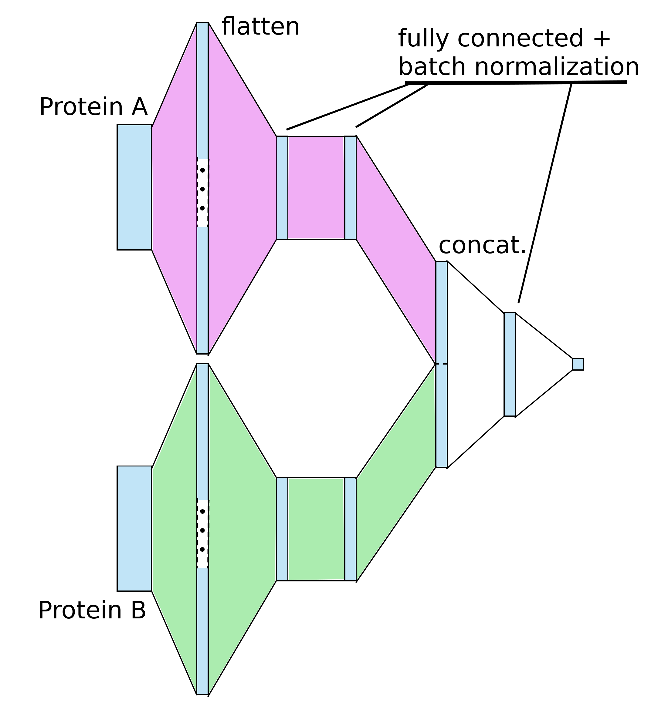
Figure 1: Our fully connected model. Parts in cyan are layers of neurons. Weights of the feature extractions part of the network are independent for Protein A (pink part) and Protein B (green part).

2.2.2 Our fully connected model architecture

We explain here the choices we made to build our models, layer by layer, starting by our fully connected model. Despite being huge compared to our dataset size, with a total of 1,121,481 parameters, this model is conceptually the simplest: features extraction is done for both proteins sequence separately by flattening inputs and feeding them to two fully connected layers. Then we concatenate these layers and process to the classification with two fully connected layers, as shown Figure 1. Each fully connected layers in the model is followed by a batch normalization layer. This allow a regulation of our model, preventing overfitting and speeding up training time. Although theoretical reasons why batch normalization help are still unclear [14], it is well-known that batch normalization and dropout layers are not giving good results when applied together [15], this is the reason why our models do not contain any dropout layers in favor of batch normalization layers. Hyper-parameters of this model are presented in Table 2. All fully connected layers have 20 units followed by a classical ReLU activation function, except for the final layer having one unit with a sigmoid activation for doing binary classification (given proteins can either interact with each other or not).

Layer	Hyper-parameters	Parameters	Output shape
Input	Sequence length=1166	-	(1166, 24)
Flatten	-	0	(27984)
Fully connected	Units=20, Activation=relu	559,700	(20)
Batch normalization	-	80	(20)
Fully connected	Units=20, Activation=relu	420	(20)
Batch normalization	-	80	(20)
Concatenation	-	0	(40)
Fully connected	Units=20, Activation=relu	820	(20)
Batch normalization	-	80	(20)
Fully connected	Units=1, Activation=sigmoid	21	(1)

Table 2: Our fully connected model hyper-parameters, parameters and tensor sizes.

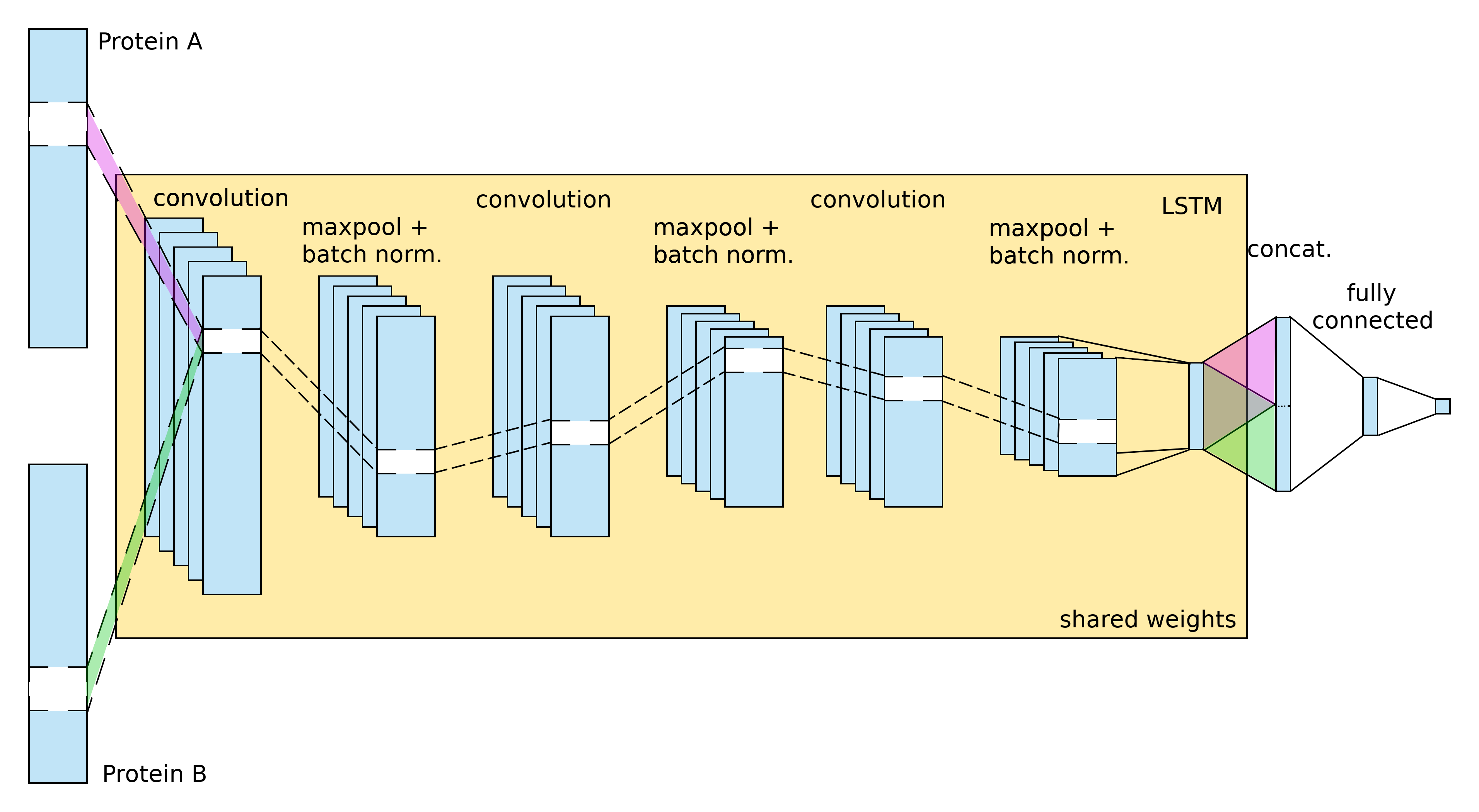
Figure 2: Our recurrent model. Parts in cyan are layers of neurons. Layers in the orange frame are sharing weights for both proteins.

2.2.3 Our recurrent model architecture

Our recurrent layers is smaller but not as straight-forward, see Figure 2. Features extraction is done for each protein by a sequence of three one-dimension convolution + pooling + batch normalization closed by a recurrent Long Short-Term Memory layer, or LSTM. Parameters of these extraction features layers are shared between our two inputs, dividing by two the number of parameters for this part of the network and reinforcing weights learning, since the same layers must deal with the chain of amino acid residues of both proteins. Indeed, there are no reasons to think that features for the first input must be different from features for the second one. The reader shall notice tha we tried to also share parameters for extraction features in our fully connected model, but this led to slightly worst results. Here, one-dimension convolutions have a kernel size of 20, see Table 3. It means the first convolution layer is looking at a window of 20 amino acids and outputs some value regarding this window, then repeats this operation by shifting its window from just one amino acid (stride of 1). Follows a pooling layer taking the convolution layer output and squashing each series of three values in a row by selecting the maximal value. The combination of these convolution and pooling layers allow both to extract the local features among successive amino acids and to significantly reduce the input shape of next layers, making the network smaller, faster to train and more prone to be generalized. Like for our fully connected model, batch normalization layers are here to both regulate and accelerate the training process. A ReLU activation function is applied after each convolution layer. Features extraction finishes with a small LSTM layer with 32 units. Like all recurrent layers, LSTM allows to extract spatial and temporal features from sequences. Since our inputs are chains of amino acid residues, there is no notion of time, but we clearly have a spatial dimension to take into account: it is reasonable to consider that amino acids arrangement is significant for having two proteins interacting each other. The series of convolution and pooling layers extract some local spatial features, but LSTM can extract global spatial features on the whole sequence by “remembering” and then considering previously treated elements. A hyperbolic tangent activation function is performed after the LSTM layer, which is also a classical choice for such layer. Once feature extraction is done, we concatenate data and give them to two fully connected layers for performing the classification. This part of the network, usually referred to be the “head” of the model, is identical to the head of our fully connected model, modulo the number of units of the first fully connected layer (here, 25),

Layer	Hyper-parameters	Parameters	Output shape
Input	Sequence length=1166	-	(1166, 24)
Convolution 1D	Filters=5, Kernel size=20, Stride=1, Activation=relu	2,405	(1147, 5)
MaxPooling 1D	Pool size=3	0	(382, 5)
Batch normalization	-	20	(382, 5)
Convolution 1D	Filters=5, Kernel size=20, Stride=1, Activation=relu	505	(363, 5)
MaxPooling 1D	Pool size=3	0	(121, 5)
Batch normalization	-	20	(121, 5)
Convolution 1D	Filters=5, Kernel size=20, Stride=1, Activation=relu	505	(102, 5)
MaxPooling 1D	Pool size=3	0	(34, 5)
Batch normalization	-	20	(34, 5)
LSTM	Units=32, Activation=tanh	4,864	(32)
Concatenation	-	0	(64)
Fully connected	Units=25, Activation=relu	1,625	(25)
Batch normalization	-	100	(25)
Fully connected	Units=1, Activation=sigmoid	26	(1)

Table 3: Our recurrent model hyper-parameters, parameters and tensor sizes. Layers in bold with cyan background are sharing weights for both inputs.

It is important to note that we also tried to represent our inputs data using an embedding layer instead of having a sparse one-hot encoding. However, using embeddings led to small accuracy improvements only, with the major drawback to greatly slowing down the training process. Typically, when our current recurrent model takes less than 2 hours to train, a recurrent model with embedding took more than 3 days to train, making harder network architecture and hyper-parameters optimizations.

3 Results

Before introducing results of our two models, we start by explaining our experimental methodology.

3.1 Methodology

Weights of each layer of our models have been initialized with Xavier uniform initialization, commonly considered to be a proper way to initialize weights at random values, even if batch normalization decrease the importance of such an initialization. Both models have been trained taking the binary cross-entropy as the loss function, using the Adam optimizer with a learning rate of 0.001 that decrease if the validation loss stays on a plateau for 5 epochs. This reduction is done by multiplying the learning rate by 0.9, and no reduction is applied once the learning rate reaches 0.0008. We train our models on batches of 2048 samples, large batch size speeding-up runtimes and favoring a good batch normalization. We use the front-end API Keras [16] with Tensorflow [17] as a back-end, and run our experiments on a NVIDIA GTX 1080 Ti GPU.

We then proceed as follows for both the regular and the strict dataset: we train our models giving a training set and a hold-out validation set, and save weights each time the validation loss reaches a new local minimum. We then evaluate our models on the validation set by taking weights where the validation loss was minimal during training, represented by dash lines in Figures 3 and 4. Notice these weights do not necessarily leads to the best validation accuracy performance, but considering the moment where validation loss is at its minimum is a good way to avoid having a model overfitting training data. Hyper-parameters optimization has been done to improve validation accuracy. These optimizations were conducted by hand, since no hyper-parameters optimization tools able to handle multiple inputs in Keras exist, up to our knowledge.

Once our hyper-parameters were fixed, we had to consider where the lowest validation loss point was reached at epoch number $x$. We performed the final tests by retraining our model on $x$ epochs taking both the training and the validation sets as our new training set, and testing our models performance on the hold-out test set. This strict methodology delivers strong robustness to information leaks, that is, avoiding to indirect overfit the validation set which would bias our models. We can then trust our final tests performances to be representative of a good generalization behavior of our models.

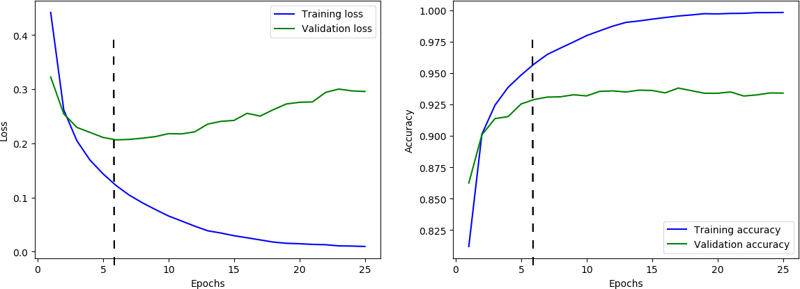
Figure 3: Training and validation losses and accuracy of our fully connected model. The dashed line represents the lowest validation loss point, where trained weights have been saved for our test results.

3.2 Fully connected model results

Table 4 shows results of our fully connected model. As expected, final test performances on the strict dataset (accuracy of 0.7625, F-score of 0.5648) are worst than on the regular dataset (accuracy of 0.8997, F-score of 0.9021). But it is more important here to consider the difference between the validation performance and the test performance on both datasets. On the regular dataset, accuracy and F-score are similar for both the validation and the test set. However on the strict dataset, test performances drop drastically when compared to validation performances, with an accuracy going from 0.9289 to 0.7625 and an F-score from 0.9278 to 0.5648 . This represents performance drops of 18% and 39%, respectively.

These results lead us to conclude that, even with hold-out validation and test sets, and even if these sets are perfectly balanced with 50% of positive and 50% of negative samples, the fully connected model is learning “by heart” that some proteins are statistically more involved into protein interactions. If such proteins appear both into the training and the test sets, the classification would be bias toward proteins that tends to interact more, instead of purely considering extracted features only to perform this classification. It is then important to consider test sets with completely new proteins for the model, going far beyond the simple fact to have test sets of new couples of proteins but where each protein appears separately somewhere in the training or the validation set.

	Regular dataset		Strict dataset
	validation set	test set	validation set	test set
Accuracy	0.9073	0.8997	0.9289	0.7625
Precision	0.9284	0.9492	0.9376	0.4269
Recall	0.8867	0.8593	0.9182	0.8345
F-score	0.9071	0.9021	0.9278	0.5648

Table 4: Results with our fully connected model

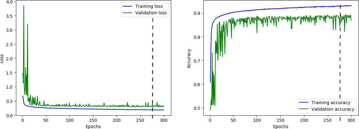
Figure 4: Training and validation losses and accuracy of our recurrent model. The dashed line represents the lowest validation loss point, where trained weights have been saved for our test results.

3.3 Recurrent model results

Table 5 shows results of our recurrent model and confirms that this model is more robust to overfitting and is generalizing better. The strict dataset being less permissive than the regular dataset, we notice performances drop between the validation and the test set, but these drops are of 12% and 26% for the accuracy and the F-score, respectively, compared to 18% and 39% for the fully connected model.

Moreover, despite having worst accuracy and F-score on the whole regular dataset and on the strict validation set than the fully connected model, our recurrent model shows significantly better performances on the strict test set, both for accuracy (0.7833 here against 0.7625 for the first model) and for the F-score (0.6502 against 0.5648).

We conclude that our recurrent model, with a 100 times less parameters than our fully connected model, generalizes better and then leads to better predictions. Its small size and its good generalization property make it a good candidate to expand it with more layers and/or more units per layers if we can train it on more data, to improve its global performance.

	Regular dataset		Strict dataset
	validation set	test set	validation set	test set
Accuracy	0.8590	0.8623	0.8899	0.7833
Precision	0.8295	0.8791	0.8892	0.5576
Recall	0.8747	0.8443	0.8854	0.7795
F-score	0.8515	0.8614	0.8873	0.6502

Table 5: Results with our recurrent model

4 Related works

In this section, we present recent related works between 2017 and 2019, applying or claiming to apply deep learning methods to prediction protein-protein interactions. We will see that it is not easy to directly compare our results to these papers, either because of a significative methodology difference or because reproducibility of these results is not possible.

Sun et al. in [18] are using stack auto-encoders to extract features from protein sequences. The classification predicting protein-protein interaction is then done by directly linking the output of the last auto-encoder to a softmax classifier. For their inputs, there are converting the sequences into fixed-size Boolean vectors, one per sequence, encoding the presence or absence of 3-grams of amino acids, i.e., each possible combination of 3 amino acids. They trained their model doing a 5-fold or 10-fold cross validation, depending their datasets.

Du et al. proposed in [19] a plain fully connected neural network, similar to our first model in this paper but significantly bigger, with layers containing 512, 256 and 128 units for what should be feature extraction, and 128 units for the head of their network. However, they are not giving as input to the network protein sequences but a list of features, such as sequence-order descriptors and composition-transition-distribution descriptors, that authors extracted themselves. They used an hold-out validation set together with a test set but then switched for a 5-fold cross validation when comparing their model with others on some other datasets.

Lei et al. use in [20] a Deep Polynomial Network on features extracted by hand, like amino acid mutation rates or hydrophobic properties of proteins, to make their classification. Thus, they do not use the chain of amino acid residues as an input. They based the learning process on a 5-fold cross validation without test sets.

In [21], Li et al. present a model composed of an embedding layer, three convolutions and a LSTM layer for feature extractions of protein sequences, before concatenating LSTM output of both proteins and performing classification with a fully connected layer linked to a sigmoid classifier. The architecture of our recurrent model is then near to their model, modulo the embedding and hyper-parameters. It is important to notice they do not mention to apply any regulation method to train their network. Their inputs are also sequence-based and they apply a 5-fold cross validation during training. with a hold-out test set. Interestingly, they also pad to zero their inputs, so they must mask these zeros into the embedding layer to make it learn something (otherwise this layer will interpret zeros as real data and their large number would prevent this layer to learn any good representation of the input). They use convolution layers after the embedding, and like for this paper, the use Keras as an API front-end to program their model. However the current implementation of convolution layers in Keras does not accept zero-masked data, and the authors do not write in their paper how did they manage to get around this technical issue.

Hashemifar et al. [22] propose a convolution-based model where feature extractions are terminated by processing data through an original randomly-initialized and untrained matrix they named "random projection module". Their model is also sequence-based but they completely transform inputs to become probabilistic position-specific profiles. To do so, they give peptide sequences to PSI-BLAST to compute these profiles. They are doing 5-fold or 10-fold cross validation, depending of datasets, and have no test sets. We observe that they are the only one tackling the protein-protein interaction prediction by doing a regression instead of a classification. This does not change fundamentally a model or its training, but it allowed them to compute precision-recall curves while focusing the analysis of their results mainly on these curves.

Finally, Zhang et al. [23] present a fully connected model regulated by dropouts. Like [19], they use composition-transition-distribution descriptors as features. They apply a 5-fold cross validation and have no separated test sets.

We can also mentioned the work of Zhao et al [24], proposing a multi-layered LSTM model to predict interface residue pair interactions, thus at a finer level level than prediction interaction between two proteins. This is a direction towards which we would like to extend our results.

4.1 Discussions

With features extracted by hand, [19, 20] and [23] are missing the point of the specificity and advantage of deep learning over classical machine learning methods: Deep Learning architectures can automatically extract features from raw data and base their training process on them. This allow machines to isolate non-trivial patterns that a human being won’t see or is not aware of.

It must be also stressed that only [19] and [22] are giving the source code of their methods (unfortunately, [19]’s source code is already unavailable) together with their experimental data (partial data for [22]). It was then not possible to directly compare methods from papers above on our data following our strict experimental methodology. Although [22]’s code is available, their paper does not give enough information about their data transformation through PSI-BLAST to do the same with our data.

None of the papers mentioned above are giving the parameter count of their model, and by judging the size of their model’s layers, they must be bigger than our large fully connected model from some orders of magnitude. However, the size of their datasets is almost always smaller than our two datasets (with the exception of a series of generated datasets from [22] with a maximum of 500,000 samples, although the exact size is not given). Those models above have then a number of parameters way above the number of training samples, making models prone to overfiting. Only [19, 18] and [21] are using hold-out final test sets, but [18] seems to give their training accuracy results instead of their test accuracy results, and they change hyper-parameters in function of the used dataset, which makes no sense to evaluate a model (hyper-parameters are part of the model). [21]’s test sets do contain positive samples only, which is a very bad way to test a model’s performance since a model always predicting interactions whatever the protein would have a 100% accuracy score.

Finally, [18] and [21] are making negative samples by taking two proteins from different subcellular locations. Although this seems to be a good idea at first glance, if negative samples are only of that nature, it may mislead the model to learn how to discriminate if proteins are from the same subcellular locations rather than if they can interact each other.

5 Conclusion

Our work on protein-protein interactions was performed with a lot of attention for dataset setup and deep learning model architecture to avoid artifacts leading to overfitting on data or to avoid deep learning workflow misuse. For the two deep learning models presented here, we were able to obtain a rather high degree of predictions with an accuracy of 76.25% for the fully-connected model and 78.33% for the recurrent model on the hold-out test set from our strict dataset, where each couple of proteins is composed of at least one protein that never appears neither in the training set nor in the validation set. These high success rates have been obtained through a more drastic methodology than other methods discussed above, in order to avoid both overfitting and information leak and thus having a model able to scale up on more data in the future. We expect our approach to be useful for the prediction of PPI for many other organisms in the perspective of whole proteome modelling.

An interesting extension of this work would be to focus on the prediction of interface residue pair interactions like in [24]. Being able to predict interactions at such a low level in sequences would bring new perspectives to the understanding of how living cells work.

References

- [1] C. Lei, H. Tao, L. Chuan, L. Lin, and L. Dandan, “Machine learning and network methods for biology and medicine,” Computational and Mathematical Methods in Medicine, vol. 2015, 2015.
- [2] E. J. Topol, “Individualized medicine from prewomb to tomb,” Cell, vol. 157, pp. 241–253, 2014.
- [3] P. Bork, C. Bowler, C. de Vargas, G. Gorsky, E. Karsenti, and P. Wincker, “Tara oceans. tara oceans studies plankton at planetary scale.” Science, vol. 348, p. 873, 2015.
- [4] M. A. Ibarra-Arellano, A. I. Campos-González, L. G. Treviño-Quintanilla, A. Tauch, and J. A. Freyre-González, “Abasy atlas: a comprehensive inventory of systems, global network properties and systems-level elements across bacteria,” Database, vol. 2016, p. baw089, 2016. [Online]. Available: http://dx.doi.org/10.1093/database/baw089
- [5] L. Strömbäck and P. Lambrix, “Representations of molecular pathways: an evaluation of sbml, psi mi and biopax,” Bioinformatics, vol. 21, no. 24, pp. 4401–4407, 2005. [Online]. Available: http://dx.doi.org/10.1093/bioinformatics/bti718
- [6] M. J. Keiser, B. L. Roth, B. N. Armbruster, P. Ernsberger, J. J. Irwin, and B. K. Shoichet, “Relating protein pharmacology by ligand chemistry,” Nature Biotechnology, vol. 25, pp. 197–206, 2007.
- [7] R. Service, “Google’s deepmind aces protein folding,” ScienceMag, 2018.
- [8] J. Shen, J. Zhang, X. Luo, W. Zhu, K. Yu, K. Chen, Y. Li, and H. Jiang, “Predicting protein–protein interactions based only on sequences information,” Proceedings of the National Academy of Sciences, vol. 104, no. 11, pp. 4337–4341, 2007.
- [9] T. Hao, W. Peng, Q. Wang, B. Wang, and J. Sun, “Reconstruction and application of protein-protein interaction network,” Int J Mol Sci, vol. 6, p. 907, 2016.
- [10] L. Tran, T. Hamp, and B. Rost, “Profppidb: Pairs of physical protein-protein interactions predicted for entire proteomes,” PLOS ONE, vol. 13, no. 7, pp. 1–13, 2018.
- [11] The UniProt Consortium, “Uniprot: the universal protein knowledgebase,” Nucleic Acids Res, vol. 45, pp. D158–D169, 2017.
- [12] B. Chapman and J. Chang, “Biopython: Python tools for computational biology,” SIGBIO Newsl., vol. 20, no. 2, pp. 15–19, Aug. 2000. [Online]. Available: http://doi.acm.org/10.1145/360262.360268
- [13] P. J. A. Cock, T. Antao, J. T. Chang, B. A. Chapman, C. J. Cox, A. Dalke, I. Friedberg, T. Hamelryck, F. Kauff, B. Wilczynski, and M. J. L. de Hoon, “Biopython: freely available python tools for computational molecular biology and bioinformatics,” Bioinformatics, vol. 25, no. 11, pp. 1422–1423, 2009. [Online]. Available: http://dx.doi.org/10.1093/bioinformatics/btp163
- [14] S. Santurkar, D. Tsipras, A. Ilyas, and A. Madry, “How does batch normalization help optimization?” in Advances in Neural Information Processing Systems (NIPS), 2018, pp. 2488–2498.
- [15] X. Li, S. Chen, X. Hu, and J. Yang, “Understanding the disharmony between dropout and batch normalization by variance shift,” arXiv:1801.05134, 2018.
- [16] F. Chollet et al., “Keras,” https://keras.io, 2015.
- [17] M. Abadi, A. Agarwal, P. Barham, E. Brevdo, Z. Chen, C. Citro, G. S. Corrado, A. Davis, J. Dean, M. Devin, S. Ghemawat, I. Goodfellow, A. Harp, G. Irving, M. Isard, Y. Jia, R. Jozefowicz, L. Kaiser, M. Kudlur, J. Levenberg, D. Mané, R. Monga, S. Moore, D. Murray, C. Olah, M. Schuster, J. Shlens, B. Steiner, I. Sutskever, K. Talwar, P. Tucker, V. Vanhoucke, V. Vasudevan, F. Viégas, O. Vinyals, P. Warden, M. Wattenberg, M. Wicke, Y. Yu, and X. Zheng, “TensorFlow: Large-scale machine learning on heterogeneous systems,” 2015, software available from tensorflow.org. [Online]. Available: https://www.tensorflow.org/
- [18] T. Sun, B. Zhou, L. Lai, and J. Pei, “Sequence-based prediction of protein protein interaction using a deep-learning algorithm,” BMC Bioinformatics, vol. 18, no. 1, p. 277, 2017.
- [19] X. Du, S. Sun, C. Hu, Y. Yao, Y. Yan, and Y. Zhang, “Deepppi: Boosting prediction of protein–protein interactions with deep neural networks,” Journal of Chemical Information and Modeling, vol. 57, no. 6, pp. 1499–1510, 2017.
- [20] H. Lei, Y. Wen, A. Elazab, E. Tan, Y. Zhao, and B. Lei, “Protein-protein interactions prediction via multimodal deep polynomial network and regularized extreme learning machine,” IEEE Journal of Biomedical and Health Informatics, 2018.
- [21] H. Li, X.-J. Gong, H. Yu, and C. Zhou, “Deep neural network based predictions of protein interactions using primary sequences,” Molecules, vol. 23, no. 8, p. 1923, 2018.
- [22] S. Hashemifar, B. Neyshabur, A. A. Khan, and J. Xu, “Predicting protein–protein interactions through sequence-based deep learning,” Bioinformatics, vol. 34, no. 17, pp. i802–i810, 2018.
- [23] L. Zhang, G. Yu, D. Xia, and J. Wang, “Protein-protein interactions prediction based on ensemble deep neural networks,” Neurocomputing, vol. 324, pp. 10–19, 2019.
- [24] Z. Zhao and X. Gong, “Protein-protein interaction interface residue pair prediction based on deep learning architecture,” IEEE/ACM Transactions on Computational Biology and Bioinformatics, 2018.