Driven spheres, ellipsoids and rods in explicitly modeled polymer solutions

Abstract

Understanding the transport of driven nano- and micro-particles in complex fluids is of relevance for many biological and technological applications. Here we perform hydrodynamic multiparticle collision dynamics simulations of spherical and elongated particles driven through polymeric fluids containing different concentrations of polymers. We determine the mean particle velocities which are larger than expected from Stokes law for all particle shapes and polymer densities. Furthermore we measure the fluid flow fields and local polymer density and polymer conformation around the particles. We find that polymer-depleted regions close to the particles are responsible for an apparent tangential slip velocity which accounts for the measured flow fields and transport velocities. A simple two-layer fluid model gives a good match to the simulation results.

Keywords: driven colloids, multiparticle collision dynamics, polymer depletion

1 Introduction

Individual colloidal particles at equilibrium undergo Brownian motion in Newtonian fluids such as water. Since the pioneering works of Einstein, Langevin and Smoluchowski, an excellent understanding of this dynamics has been developed [1]. By contrast, the random motion of colloids in complex fluids such as polymer solutions and gels, and in biological fluids and cells, is by far less well understood although considerable progress has been made in this research field during the last decades, both from the experimental and the theoretical perspective (see, for example Refs. [2, 3, 4, 5, 6]). Even more challenging is understanding colloidal motion in complex fluids driven out of equilibrium by, for example, external forces or fluid flow [7], or if the system is intrinsically out of equilibrium as in the case of active colloids [8, 9].

Understanding the motion of colloidal particles through polymer solutions and polymeric or filamentous networks is of considerable importance in colloid science and for biomedical applications. For example, using colloidal particles to probe the physical properties of the crowded environment of living cells has been used to distinguish healthy cells from cancer cells [10]. Moreover, there is considerable interest in understanding the motion of nano- and micro-particles through biological gels such as mucus which line many of the body cavities, for example the lungs and the stomach [11, 12, 13, 14, 15, 16]. In order to understand how different particles – proteins, viruses, drugs, and food particles – cross biological barriers several experimental studies of particle diffusion through mucus have been performed [11, 12, 13, 17, 20, 14, 15, 18, 16, 19]: However, many conventional drugs become trapped in the mucus layer due to steric hindrance or short-range adhesive forces [21] and therefore it is of high relevance to design new ways of efficiently delivering drugs based on nanoparticles, which could more efficiently cross the mucus barrier [13], or move through other biologically complex body fluids such as the extracellular matrix [21].

Simple, diffusion-limited motion in complex fluids is usually too slow for efficient transport. A way to overcome this is to use magnetic particles which can be driven by external magnetic forces to specific target regions [23, 22]. Other ways to drive nano- or micro-particles through polymeric fluids are to use optical driving forces [24, 14] or simply sedimentation [25]. When a colloid moves in a Newtonian medium of viscosity $\eta$, the expectation is that the velocity $V$ follows Stokes formula, $V=F/(6\pi\eta a)$, with $F$ the driving force and $a$ the radius of the particle. However, Koenderink et al. showed experimentally that particles driven by sedimentation in macromolecular xanthan solutions move faster than expected [25]. This result has been explained theoretically by the occurrence of an apparent slip velocity, experienced by the driven particles because they are surrounded by a uniform polymer-depleted region [26, 27]. However, the density of polymers around a driven particle can be highly non-uniform, as shown for a colloid dragged through a macromolecular solution of $\lambda$-DNA with optical tweezers [24]. Theories have also tried to take into account the effect of local fluid flow around moving particles, using for example the concept of dynamic depletion for protein transport in polymer solutions [28]. Lattice models have recently been used to characterize the transport of a driven particle in simplified crowded environments [29].

Mesoscale simulations provide a way of investigating the underlying microscopic mechanisms relevant for colloidal motion in polymeric fluids, but currently there are very few simulations of driven colloids in simple polymer solutions [30, 24]. It has been demonstrated that multiparticle collision dynamics (MPCD) is an efficient method to simulate fluctuating hydrodynamics of colloids (see, e.g. [31, 32]) and polymers (see, e.g. [33, 34, 35, 36, 37, 38, 39]). So far colloid-polymer suspensions at equilibrium have been studied with MPCD in Refs. [40, 41, 42]. Here we perform coarse-grained hydrodynamic simulations of driven spheres, ellipsoids and rods moving in a fluid that contains varying concentrations of explicitly modeled, ‘bead-spring’ polymers.

Besides the transport velocities, we determine the fluid flow around the particles and the detailed local polymer properties. Hence we are able to identify the relevant mechanisms for enhanced colloidal transport in polymer solutions. In Sec. 2 we introduce the simulation method, and we present our results in Sec. 3. We summarise our work in Sec. 4.

2 Methods

We model the hydrodynamics and fluctuations of the background Newtonian fluids using multiparticle collision dynamics. To simulate polymeric fluids we couple coarse-grained, bead-spring polymers to the solvent. The dynamics of the fluid particles and the colloids is performed using molecular dynamics (MD) simulations.

2.1 Multiparticle collision dynamics (MPCD)

The Newtonian background fluid is simulated using MPCD. This is a coarse-grained solver of the Navier Stokes equations which includes thermal fluctuations [43, 44]. The fluid is modeled by point-like, effective fluid particles of mass $m$ which perform alternate streaming and collision steps. In the streaming step fluid particles move ballistically for a time $\delta t$ so that their positions $\mathbf{x}_{i}$ are updated to

$$\mathbf{x}_{i}(t+\delta t)=\mathbf{x}_{i}(t)+\mathbf{v}_{i}(t)\delta t$$ (1)

where $\mathbf{v}_{i}$ are their velocities. They are then sorted into cubic cells of length $a_{0}$ and, in the collision step, all particles in a cell exchange momentum according to

$$\mathbf{v}_{i}(t+\delta t)=\mathbf{v}_{\xi}(t)+\mathbf{v}_{\textnormal{rand}}(t)+\mathbf{v}_{P}(t)+\mathbf{v}_{L}(t)$$ (2)

where $\mathbf{v}_{\xi}$ is the instantaneous average velocity in the cell, $\mathbf{v}_{\textnormal{rand}}$ is a random velocity drawn from a Maxwell-Boltzmann distribution at temperature $T$, and $\mathbf{v}_{P}$ and $\mathbf{v}_{L}$ ensure local linear and angular momentum conservation, respectively [44]. As basic units in the simulations we chose length $a_{0}$, mass $m$ and energy $k_{B}T$. We use $\delta t=0.02\sqrt{ma_{0}^{2}/k_{B}T}$ and a fluid particle number density $n=10a_{0}^{-3}$ in order to model viscous flow at low Reynolds number. In the absence of polymers the viscosity is then $\eta_{0}=16.04\sqrt{mk_{B}T/a_{0}^{4}}$.

Table 1: Simulation parameters.

• $\frac{a}{a_{0}}$	$\frac{b}{a_{0}}$	$\epsilon_{1}$	$\epsilon_{2}$	description	$\frac{S_{x}}{a_{0}}$	$\frac{S_{y}}{a_{0}}$	$\frac{S_{z}}{a_{0}}$	$N_{t}$	$\frac{F}{a_{\text{eff}}(k_{B}T/a_{0}^{2})}$	$k_{b}/k_{B}T$	symbol/color code
  3	3	1	1	sphere	48	48	48	70K	5	0
  3	3	1	1	sphere	48	48	48	70K	5	12
  3	6	1	1	short ellipsoid	48	48	60	90K	5	0
  3	9	1	1	long ellipsoid	48	48	120	180K	5	0
  3	6	0.5	1	short rod	48	48	60	90K	5	0
  3	6	0.5	1	short rod	48	48	60	60K	10	0
  3	6	0.5	1	short rod	48	48	60	45K	15	0
  3	6	0.5	1	short rod	48	48	60	30K	20	0
  3	6	0.5	1	short rod	48	48	60	25K	25	0
  3	9	0.5	1	long rod	48	48	120	180K	5	0

2.2 Polymer model

To simulate polymeric fluids, we add simple bead-spring polymers to the Newtonian background fluid. Each polymer consists of $N=12$ beads of diameter $\sigma=a_{0}$ which are located at positions $\mathbf{r}_{i}$, $i=1,\dots,N$. Individual beads are connected by a stiff bond potential

$$V_{\textnormal{bond}}=\frac{1}{2}k_{\textnormal{bond}}\sum_{i=2}^{N}(|\Delta\mathbf{r}_{i}|-l_{0})^{2}$$ (3)

with $\Delta\mathbf{r}_{i}=\mathbf{r}_{i}-\mathbf{r}_{i-1}$, $l_{0}=a_{0}$ and $k_{\textnormal{bond}}=10^{5}k_{B}T/a_{0}^{2}$. In some cases we include a bending potential

$$V_{\textnormal{bend}}^{P}=\frac{1}{2}k_{\textnormal{b}}\sum_{i=3}^{N}\left(\frac{\Delta\mathbf{r}_{i}\cdot\Delta\mathbf{r}_{i-1}}{|\Delta\mathbf{r}_{i}||\Delta\mathbf{r}_{i-1}|}-1\right)^{2}$$ (4)

with $k_{b}=12k_{B}T$ in order to simulate semi-flexible polymers, but we mainly study systems of flexible polymers where $k_{b}=0$.

We use a purely repulsive soft Weeks-Chandler-Anderson (WCA) potential [45] between polymer beads,

$$V_{\textnormal{WCA}}(r)=4\epsilon\left[{\left(\frac{\sigma^{\ast}}{r}\right)}^{12}-{\left(\frac{\sigma^{\ast}}{r}\right)}^{6}\right]+\epsilon$$ (5)

for $r<2^{1/6}\sigma^{\ast}$ and zero otherwise. Here $r$ is the distance between the beads, and we use $\epsilon=k_{B}T$ and $\sigma^{\ast}=\sigma/2^{1/6}$. We consider fluids at different polymer volume fractions $\rho=\{0.01,0.05,0.1,0.2\}$ with $\rho=N_{p}N\pi\sigma^{3}/(6V_{d})$ where $N_{p}$ is the number of polymers in the simulation and $V_{d}$ the simulation domain volume. The polymers are initially randomly distributed in the simulation box, but are not allowed to overlap with the solid particles.

2.3 Colloidal spheres, spheroids and rods

We use three different types of solid particles immersed in the polymeric fluids, namely (i) spheres of radius $a$, (ii) ellipsoids with semi-minor axis $a$ and semi-major axis $b$, and (iii) rods of length $2b$ and width $2a$, modeled as a superellipsoid [46, 47, 48]. The surface of the superellipsoid at time $t=0$ is given by

$$\left[\left(\frac{x-x_{0}}{a}\right)^{\frac{2}{\epsilon_{2}}}+\left(\frac{y-y_{0}}{a}\right)^{\frac{2}{\epsilon_{2}}}\right]^{\frac{\epsilon_{2}}{\epsilon_{1}}}+\left(\frac{z-z_{0}}{b}\right)^{\frac{2}{\epsilon_{1}}}=1$$ (6)

and its center is located at ($x_{0},y_{0},z_{0}$). For $\epsilon_{1}=1$ and $\epsilon_{2}=1$ Eq. (6) reduces to the equation of a conventional ellipsoid with semi-minor axis $a$ and semi-major axis $b$, and if in addition $b=a$, to a sphere. In order to model rods, we use $\epsilon_{1}=0.5$ while we keep $\epsilon_{2}=1$, which means that their cross section is circular. All the particle dimensions we studied are listed in Table 1.

To drive the colloids, we apply a force $\mathbf{F}(t)=F\mathbf{n}(t)$ where $\mathbf{n}(t)$ is the instantaneous unit orientation vector pointing along the long axis of the particle. This is initially along the negative $z$ direction (Eq. (6)). The direction of the particle orientation remains constant in time for spheres, but not for the other particle shapes. In order to obtain approximately the same transport velocity for differently shaped colloids, we normalize the magnitude of the applied force, $F>0$, by the effective radius $a_{\text{eff}}$ of a particle, defined by $a_{\text{eff}}=\sqrt[3]{3V_{p}/4\pi}$ where $V_{p}$ is the volume of the particle.

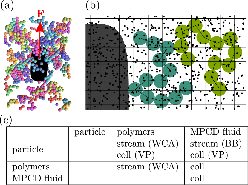
Figure 1: (a) Simulation snapshot around a solid particle (black) driven by a constant force $\mathbf{F}$ through a polymer solution. Different colors of the individual polymers are to aid visualization. (b) 2D sketch of the components involved: driven particle (grey), polymers (light and dark green), MPCD fluid particles (black dots) including virtual particles (VP; black dots in solid particle). The rectangular collision cell grid, which is shifted randomly in every time step [44], is also shown. (c) overview of the interactions between the different components in the streaming and collision step. Short range forces are realized by WCA potentials and bounce-back (BB) [49].

2.4 Hybrid MPCD-MD simulations

To simulate the dynamics of the polymers and the solid particles in the MPCD fluid we use a hydrid MPCD-MD scheme [44, 49]. In parallel with the MPCD streaming step the positions and velocities of the polymer beads are updated by determining the forces from the potentials [Eqs. (3) - (5)] and using a Velocity Verlet algorithm [50] with time step $\delta t_{P}=0.002\sqrt{mh^{2}/k_{B}T}$. The polymer beads, which have masses $m_{P}=10m$, are coupled to the fluid by including them in the collision step [33].

The colloid dynamics is also evolved using a Velocity Verlet algorithm, but with a time step $\delta t_{B}=0.02\sqrt{mh^{2}/k_{B}T}$. Fluid particles interact with the colloids by applying a bounce back rule, with momentum and angular momentum exchanged accordingly. In order to accurately resolve the flow fields near the colloids we use virtual particles inside the colloids, which contribute to the MPCD collision step [44]. In addition, polymer beads interact with the solid particles via a soft repulsive potential. A sketch of the simulated system including an overview of the interactions between the different components involved are shown in Fig. 1.

For all the systems studied we chose the simulation box sizes in the $x$ and $y$ directions to be $S_{x}=S_{y}=48$, while varying $S_{z}$ such that elongated particles minimized self-interaction due to long-range hydrodynamic interactions, see Table 1. In addition, we included two hard, impenetrable no-slip walls, located at $z=\pm S_{z}/2$, in order to suppress the tendency of the system to self-accelerate [51]. For each simulation a single solid particle is placed inside the simulation box. It is initialized at position $z_{0}=+S_{z}/4$, $x_{0}=y_{0}=0$ so that it is not too close to the walls. The number of simulation streaming and collision time steps $N_{t}$ (see Table 1) is adapted so that particles move to a final position $z_{0}\approx-S_{z}/4$. For each system we average over many realizations, i.e. between 20 and 65, in order to get good statistics for the measured physical quantities.

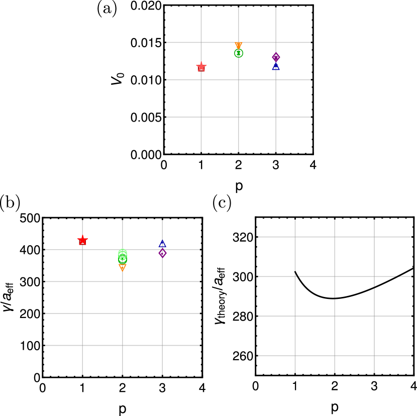
Figure 2: (a) Velocity $V_{0}$ of the differently-shaped colloids in the absence of polymers as a function of the colloid aspect ratio $p$. (b) Friction coefficient/effective radius determined from MPCD simulations for different colloid shapes. (c) Theoretical prediction for the friction coefficient/effective radius for prolate ellipsoids. Symbol/color code as in Table 1.

3 Results

3.1 Velocities: no polymers

We first determine the time- and ensemble-averaged velocity $V_{0}$ of the colloids in the absence of polymers ($\rho=0$) for all the systems listed in Table 1. In Fig. 2(a) we show results for different particle geometries, but keeping the driving force per effective radius $F/a_{\text{eff}}=5k_{B}T/a_{0}^{2}$ constant. Here $F$ is chosen rather small in order to simulate low Reynolds number flows. We also plot, in Fig. 2(b), the corresponding friction coefficients, ${\gamma}/{a_{\text{eff}}}={F}/{(a_{\text{eff}}V_{0}})$.

As expected, by normalizing the driving force by a colloid’s effective radius $a_{\text{eff}}$, the velocities and friction coefficients of all particles (spheres, ellipsoids and rods) are approximately the same. There is, however, a small dependence on the particle aspect ratio $p=b/a$ (Fig. 2(a)). One reason for the dependence of $V$ on $p$ is that for ellipsoids the translational hydrodynamic friction coefficient, parallel to the long axis of the particles, divided by the effective radius, ${\gamma_{\text{theory}}}/{a_{\text{eff}}}$, has a small dependence on the aspect ratio $p$ [52],

$$\frac{\gamma_{\text{theory}}}{a_{\text{eff}}}=\frac{16\pi\eta p^{-\frac{1}{3}}}{\frac{2p}{1-p^{2}}+\frac{\left(2p^{2}-1\right)\log\left(\frac{\sqrt{p^{2}-1}+p}{p-\sqrt{p^{2}-1}}\right)}{\left(p^{2}-1\right)^{3/2}}}.$$ (7)

This dependence on $p$ is illustrated in Fig. 2(c).

Simulations show the same trend for the dependence of the friction coefficient on $p$ as in the simulations, i.e.  a minimum for aspect ratio $p=2$. However, in the simulations, the dependence on $p$ is stronger than the theoretical prediction, and the absolute values of the friction coefficients are larger than the theoretical ones. The most likely reason for the differences is that we do not simulate an infinite domain of fluid, but use periodic boundary conditions for the simulations to be feasible, which can have an impact on the absolute values of the measured friction coefficients [32]. More simulations are needed to investigate this further. However, in the following we will only consider relative, rather than absolute trends in the velocities.

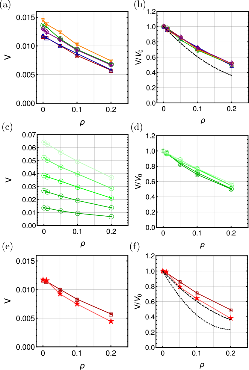
Figure 3: (a) Time- and ensemble-averaged velocities $V$ as a function of polymer concentration $\rho$ for differently-shaped colloids moving in flexible polymer solutions ($k_{b}=0$, $N=12$). The driving force $F$ is scaled by the effective radius $a_{\text{eff}}$ of the particle: $F/a_{\text{eff}}=5k_{B}T/a_{0}^{2}$. (b) Data in (a) with velocities scaled by the zero polymer limit, $V_{0}$. The black dashed line shows the theoretical curve based on simple viscosity scaling. (c) Velocities $V$ for short rods for different driving forces $F/a_{\text{eff}}$ as a function of polymer concentration $\rho$. (d) Data in (c) with velocities scaled by the zero polymer limit, $V_{0}$. (e) Velocities $V$ for spheres for different polymer flexibilities as a function of polymer concentration $\rho$. (f) Data in (e) with velocities scaled by the zero polymer limit, $V_{0}$. The black dashed line is the same as in (b). The black dotted line shows the theoretical curve based on simple viscosity scaling for motion in semiflexible polymer solutions. Symbol/color code as in Table 1.

3.2 Velocities: varying the polymer density

We now add polymers to the fluid, and observe that the velocities $V$ of the colloids decrease with increasing polymer density $\rho$. This is shown in Fig. 3, where again we use a driving force $F/a_{\text{eff}}=5k_{B}T/a_{0}^{2}$. In Fig. 3(a) we plot the velocities for spheres, ellipsoids and rods moving in fluids containing flexible polymers ($k_{b}=0$), which all decay in a similar way. This is seen more clearly by plotting the rescaled velocities $V/V_{0}$ against the density $\rho$ in Fig. 3(b).

Since in Newtonian fluids the friction coefficients increase linearly with the fluid viscosity $\eta$ (see e.g. Eq. (7)), the decrease in colloid velocity could simply be due to the increase in viscosity with the addition of polymers. If this is indeed the case, the velocity of the particle should scale with the the inverse viscosity $\eta^{-1}$. In Ref. [48] we determined the polymer density-dependence of the viscosity using shear-rheology measurements. For example, for flexible polymers ($k_{b}=0$) of length $N=12$, the density-dependence of the inverse viscosity can be fitted to the curve $\eta^{-1}=\eta_{0}^{-1}(1-4.74\rho+7.75\rho^{2})$, which is plotted as a black dashed line in Fig. 3(b). Thus we see that the measured velocities are larger than those predicted by a simple viscosity scaling. We shall show later that the reason for the discrepancy lies in the structure of the polymeric fluids.

We also measured the dependence of the particle velocity on the driving force $F$, as shown in Fig. 3(c). $F$ was increased up to $F/a_{\text{eff}}=25k_{B}T/a_{0}^{2}$, where the velocities increase up to $V=0.065\sqrt{k_{B}T/m}$, corresponding to a Reynolds number $Re=bV/\nu\approx 0.4$ (using the kinematic viscosity $\nu=1.6\sqrt{k_{B}Ta_{0}^{2}/m}$). As shown in Fig. 3(d), the scaled velocities $V/V_{0}$ almost collapse to a single curve showing that the driving force indeed only has a minor effect on the mobility of the particles. The velocities are, however, slightly higher when using larger driving forces. As we will see below, this is probably caused by the distribution of polymers around the particles.

Finally we contrast, in Figs. 3(e) and (f), the velocities of spheres moving in two different polymeric fluids, containing flexible or semiflexible filaments, respectively. The decay of the velocity $V$ for the sphere moving in the semiflexible polymer solutions is stronger than for flexible polymers. The main reason for this is that the viscosities of the semiflexible solutions increase more rapidly with density than those of the flexible solutions [48]. However, again, the sphere velocities are larger than expected from a simple viscosity scaling based on the relation $\eta^{-1}=\eta_{0}^{-1}(1-7.70\rho+19.4\rho^{2})$ measured for the semiflexible polymers (see the black dotted curve in Fig. 3(f)).

Taken together, these results show that the effective mobilities of driven spheres, ellipsoids and rods in a polymeric fluid are larger than those expected from modelling the fluids as a simple continuum viscous medium. We shall now investigate the relation between the structure of the polymeric fluids and the particle velocities.

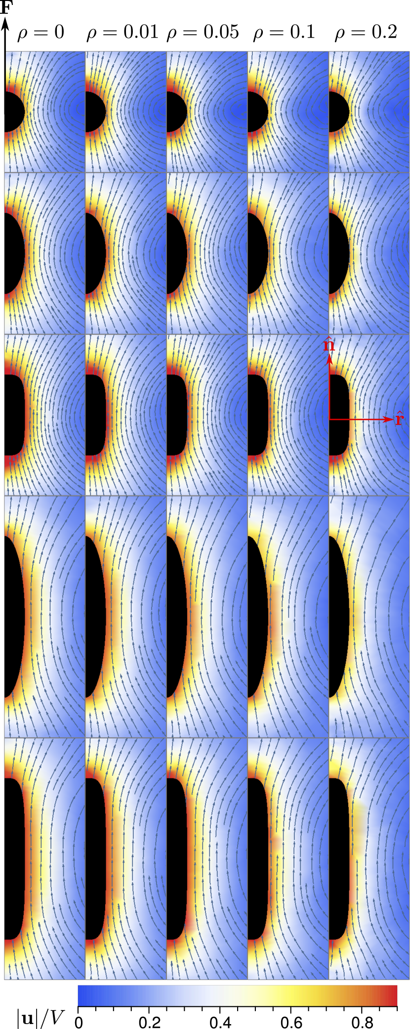
Figure 4: Time-, ensemble- and azimuthally averaged flow fields around the different types of colloid (top to bottom) moving in fluids containing flexible polymers of different volume fraction $\rho$. Streamlines are shown by blue arrows, and the background color (red to blue) of the plot indicates the strength of the flow field $|\mathbf{u}|$.

3.3 Flow fields

To help to understand why the colloids move faster than expected, we measure the velocity fields around them. It is well known that in a Newtonian fluid a particle driven by a constant force at low Reynolds number creates a Stokeslet flow in the far field, which decays with distance $r$ as $r^{-1}$ [52]. These long-range flows enable for example sedimenting particle suspensions to interact hydrodynamically and to create large-scale motion [53]. Details of the near-field flow are determined by the shape of the particle.

In Fig. 4 we show the time-, ensemble- and azimuthally averaged flow fields $\mathbf{u}(\mathbf{r})=u_{n}\hat{\mathbf{n}}+u_{r}\hat{\mathbf{r}}$ around single particles driven by a constant force $\mathbf{F}=F\hat{\mathbf{n}}$ with $F/a_{\text{eff}}=5k_{B}T/a_{0}^{2}$. The first column displays the flow fields in the absence of polymers, and the other columns the flow fields for solutions containing flexible polymers ($k_{b}=0$, $N=12$) at different volume fractions $\rho$. We observe that in all cases the flow fields show a Stokeslet-like behavior away from the particles. In the near field there are strong tangential flows, particularly for the more elongated particles. In Fig. 4 the strengths of the flow fields $|\mathbf{u}|$ are all normalized to the mean velocities $V$ of the particles. While their overall shapes do not change significantly with increasing the polymer density, we do observe that the scaled flow field strength is somewhat suppressed for particles moving in high-density polymeric fluids (e.g. right column with $\rho=0.2$).

To investigate the differences of the flow fields with and without polymers in more detail, we non-dimensionalize the parallel flow field components $u_{n}$ with the corresponding particle velocity, defining $u_{e}=u_{n}/V$ for the simulation with polymers, and $u_{e}^{0}=u_{n}^{0}/V_{0}$ for the no-polymer case. In Fig. 5(a) we plot the distance-dependent decays of the ratio $u_{e}(r)/u_{e}^{0}(r)$ measured around the equator of the particle for long rods ($b=9a_{0}$) for different polymer densities $\rho$. These results show that the flow fields in the presence of polymers decay more quickly close to the colloid than in the polymer-free case. This effect becomes more pronounced with increasing polymer density. By contrast, far from from the particle the ratio $u_{e}(r)/u_{e}^{0}(r)$ levels off to a constant $I$ indicating an $r^{-1}$ scaling in all cases. Similar curves are obtained for the other particle shapes although for the spherical particles the flow field ratio does not level off so clearly to a constant. This is because of the finite simulation box which induces recirculation flows which are strongest for the spherical particles, see Fig. 4.

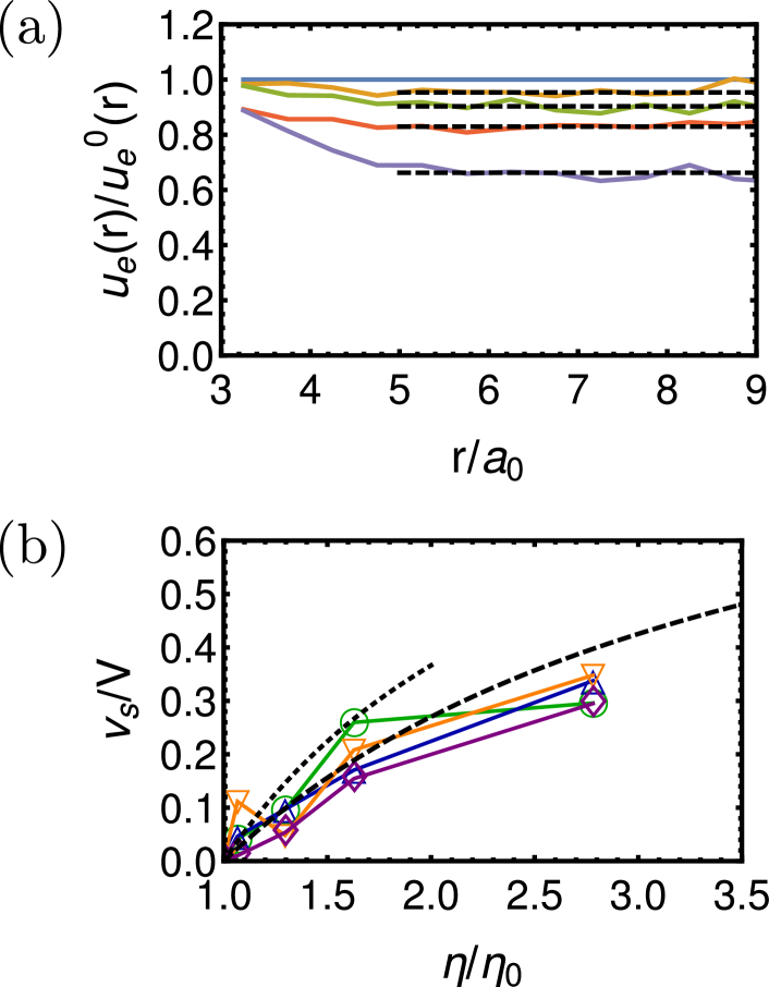
Figure 5: (a) Decay of the ratio of the non-dimensionalized tangential flow fields $u_{e}(r)$ and no-polymer flow fields $u_{e}^{0}(r)$. The curves, for densities $\rho=0.01$ (orange), $\rho=0.05$ (green), $\rho=0.1$ (red) and $\rho=0.2$ (purple), level off to constants $I$ (fits shown as black dashed lines). (b) Measured apparent slip velocities $v_{s}/V=1-I$ as a function of the normalized bulk viscosities $\eta/\eta_{0}$ of the fluids. The black dotted and dashed lines show theoretical predictions from a two-fluid model with inner fluid-layer thickness $\delta=a_{0}$ and $\delta=0.5a_{0}$, respectively. Symbol/color code as in Table 1.

The shape of the flow field can be modelled by introducing an apparent slip velocity $v_{s}=(1-I)V$ at the surface of the particle [54]. The slip velocities for differently-shaped colloids are shown in Fig. 5(b) as a function of the scaled viscosity of the polymer solution. To understand the reasons for this effective slip around the colloids we next study the properties of the polymers in their vicinity.

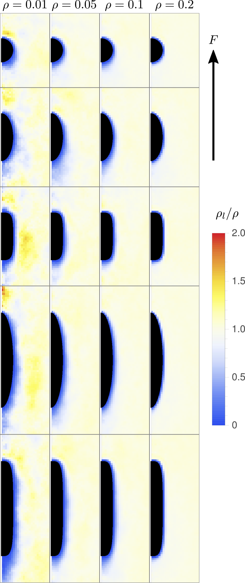
Figure 6: Local polymer density around different types of particles and at different bulk polymer densities $\rho$. The blue layers around the particles indicate polymer-depleted regions. Yellow indicates polymer-rich regions in front of and next to the particles.

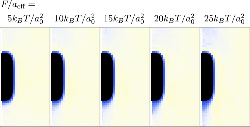
Figure 7: Local polymer density for short rods at different driving forces $F/a_{\text{eff}}$ for $\rho=0.2$. Color code as in Fig. 6.

3.4 Local polymer density and the depletion layer

Explicitly modeling the dynamics of polymers allows us to obtain detailed information about their spatial distribution and their conformations. In Fig. 6 we show the time-, ensemble- and azimuthally averaged local polymer densities, $\rho_{l}$, around the differently-shaped colloids for polymer solutions of flexible filaments, and using a driving force $F/a_{\text{eff}}=5k_{B}T/a_{0}^{2}$.

First, it can be seen from Fig. 6 that at high mean polymer density $\rho=0.2$ (right column) the distribution of polymers around all the colloids looks very similar: there is a shallow layer of fluid around the particle (blue region) where the local polymer density is significantly reduced. This layer is of almost constant thickness, and in particular there is no clear front-back asymmetry.

This changes significantly when $\rho$ is reduced. The thickness of the low-polymer-density layer increases, and a relatively large polymer-poor region emerges behind the colloids. For very small $\rho$ (left column) regions of enhanced polymer density in front of and next to the particles also appear. The reason for this is that polymers are pushed forward by the moving colloid, leading to an enhanced polymer density in front of the particle. This then tends to get pushed sideways leading to the polymer-rich regions at the side of the colloid. As the polymers are displaced the moving colloid leaves a polymer-poor area behind, since the polymers need time to diffusively re-enter this region.

For $F/a_{\text{eff}}=5k_{B}T/a_{0}^{2}$ these effects do not occur at high densities because polymer diffusion and interactions quickly remove any gradients in polymer density. However using higher driving forces, $F$, can lead to significant polymer-poor regions behind the particle even at higher polymer densities, as shown in Fig. 7 for $\rho=0.2$. The length of the polymer-poor region increases with increasing $F$, as the advective transport of the particles becomes faster than the diffusion of the polymers. This effect could contribute to the small differences in the transport velocities at different driving forces, see Fig. 3(d).

Finally, the reason for the low-polymer-density layer around the particle is the finite size of the polymers. At low polymer densities polymer depletion layers at surfaces are of the order of the radius of gyration of the polymers [55]. This is also the case for our polymers ($N=12$) where the radius of gyration is approximately $r_{g}\approx 2a_{0}$: at very low polymer densities (left column of Fig. 6), this is the order of the size of the depletion layer. At higher densities polymer-polymer interactions lead to configurations where the monomers are much more uniformly distributed around the particle leading to a smaller depletion layer thickness.

A more detailed representation of the polymer distribution around the equator of the colloids is shown in Fig. 8. From Fig. 8(a) we can see that at relatively low bulk polymer density $\rho=0.05$ the polymer density very close to the particle is zero, which means that the local fluid viscosity there is simply $\eta_{0}$, the fluid viscosity for the no-polymer case. Then the density of polymers increases gradually, and in a similar way for all particles considered, to eventually reach the bulk plateau. The depletion layer thickness, defined as the distance from the particle where the polymer density has dropped to half its value, $\delta=r(\rho_{l}/\rho=0.5)-a$, is here around $\delta\approx a_{0}$ and hence for $\rho=0.05$ already smaller than the radius of gyration. For higher polymer densities the depletion layer thickness decreases, as shown for the highest density $\rho=0.2$ in Fig. 8(b). Here $\delta\approx 0.5a_{0}$, which is the radius of a monomer. This is what we expect at high densities, where dense polymer solutions are expected to arrange uniformly due to polymer-polymer interactions, and in our coarse-grained model the monomer size defines the depletion thickness. Again, this is very similar for all the different colloids considered.

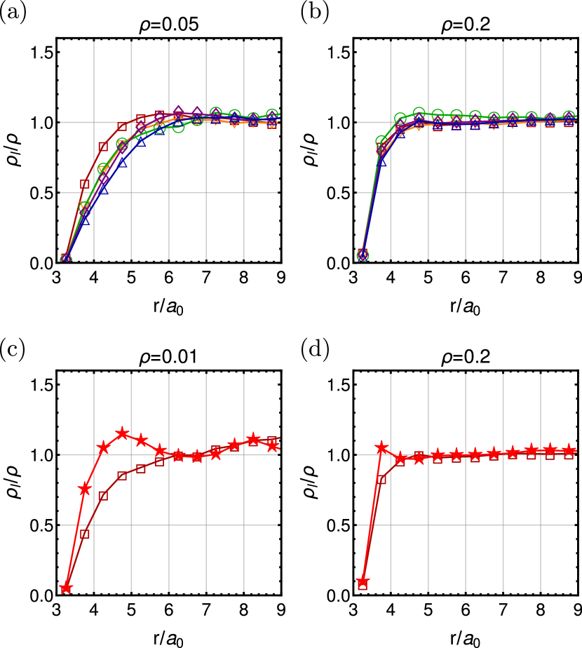
Figure 8: Local polymer densities $\rho_{l}$ normalized by the bulk densities $\rho$. Differently-shaped colloids at polymer densities (a) $\rho=0.05$ and (b) $\rho=0.2$. Colloidal spheres in flexible and semiflexible polymer solutions at polymer densities (c) $\rho=0.01$ and (d) $\rho=0.2$. Symbol/color code as in Table 1.

We do, however, see an effect of the type of polymer on the depletion layer. To show this, we compare results for motion in flexible ($k_{b}=0$) and semiflexible ($k_{b}=12k_{B}T$) polymer solutions. While for flexible polymers the radius of gyration is a good measure to estimate the depletion layer thickness at low densities, semiflexible polymers create a smaller depletion layer, comparable to the monomer size, see Fig. 8(c). At high densities the thickness is again comparable, as shown in Fig. 8(d), since it is now determined by the monomer size for both the flexible and semiflexible cases.

3.5 Other effects

So far we have seen that the polymer distribution close to the driven particles is clearly non-uniform. We also checked other local polymer properties around the particles, such as the local aligning and stretching of the polymers. However, because we mainly use rather small driving forces, $F/a_{\text{eff}}=5k_{B}T/a_{0}^{2}$, the local polymer properties around the particle are not changed significantly.

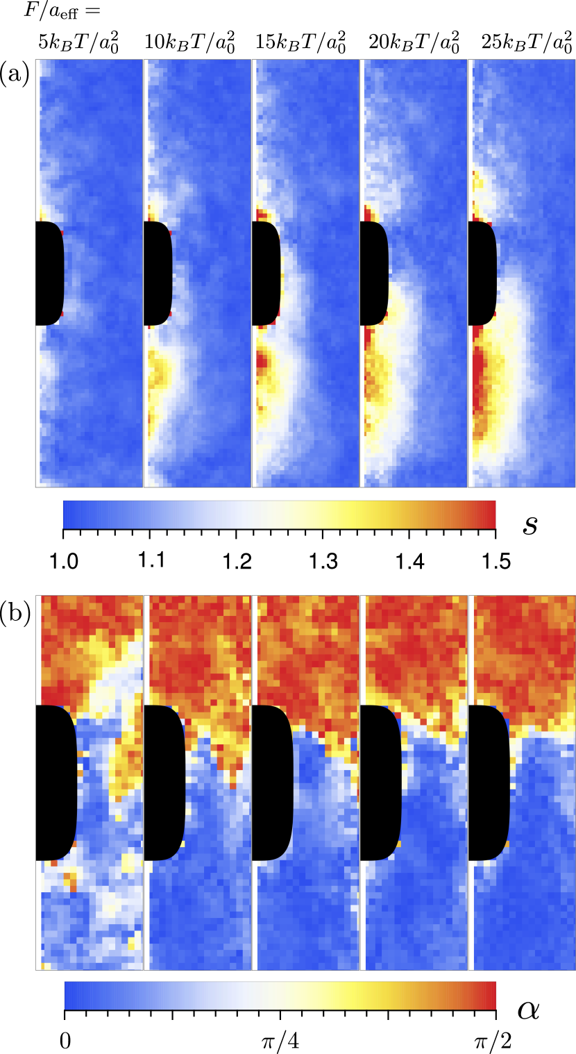
Figure 9: (a) Local effective polymer aspect ratio $s$ [Eq. (10)] for different driving forces $F/a_{\text{eff}}$. (b) Corresponding effective local orientation angle $\alpha$ of the polymers ($\alpha=0$: parallel, $\alpha=\pi/2$: perpendicular to particle orientation.)

For larger $F$ we do see some polymer stretching in front of the particle. In order to quantify the degree of stretching of the polymers, we determine the gyration tensors

$$g_{ij}=\frac{1}{N}\sum_{k=1}^{N}\Delta r_{k,i}\Delta r_{k,j}$$ (8)

for all polymers, at all times and for all different simulation runs, where $k$ is the polymer bead index, and $i$ and $j$ indicate Cartesian components of the relative vector $\Delta\mathbf{r}_{k}=\mathbf{r}_{k}-\mathbf{r}_{c}$ with $\mathbf{r}_{c}$ being the center of mass of the polymer. We then compute the local gyration tensors around the particle, averaged over time, ensembles and azimuthal angles,

$$G_{mn}(r,z)=\left\langle A_{mi}(\hat{\mathbf{n}})g_{ij}A_{jn}^{T}(\hat{\mathbf{n}})\right\rangle$$ (9)

where the transformation matrix $A_{mi}$ depends on the instantaneous particle orientation $\hat{\mathbf{n}}(t)$ and transforms the individual gyration tensors $g_{ij}$ to a coordinate system where the particle orientation $\hat{\mathbf{n}}(t)$ is the first basis vector. In Eq. (9) we averaged over all $g_{ij}$ calculated from polymer beads located within radial distances $r$ and $r+\delta r$, and within longitudinal distances $z$ and $z+\delta z$ from the center of the particle. This allows us to not only compute the local eigenvalues $\lambda_{1}^{2}(r,z)<\lambda_{2}^{2}(r,z)<\lambda_{3}^{2}(r,z)$ of $G_{mn}(r,z)$, but also the averaged orientations of the normalized eigenvectors $\hat{\mathbf{v}}_{m}(r,z)$ with respect to the particle orientation $\hat{\mathbf{n}}$. We measure the strength of the local stretching by the effective polymer aspect ratio $s(r,z)\geq 1$ defined by

$$s(r,z)=\frac{\lambda_{1}}{(\lambda_{2}+\lambda_{3})/2}$$ (10)

which is $s\approx 1$ for isotropic conformations and $s\rightarrow\infty$ for highly stretched polymers.

In Fig. 9(a) we plot $s$ for the motion of short rods at polymer density $\rho=0.2$ for different driving forces $F$. We can see that polymers get stretched mainly at the back and in front of the particle, and this effect increases with $F$. However, the overall effect is rather small for all forces ($s\lesssim 1.5$). In order to see how polymers align with respect to the particle orientation $\hat{\mathbf{n}}$ we compute the local angle $\alpha$ between $\hat{\mathbf{n}}$ and the eigenvector $\hat{\mathbf{v}}_{1}$ corresponding to the largest eigenvalue $\lambda_{1}^{2}$ which is in our transformed coordinate system simply $\alpha=\arccos|\hat{v}_{1,x}|$. In Fig. 9(b) we can clearly see that in front of the particle the polymers become oriented perpendicular to the particle due to the moving particle compressing these polymers. In contrast, polymers are aligned parallel to the particle at the back because the polymers gain extra space to move in the direction of the particle orientation.

3.6 Two-fluid model

Our results suggest that it might be possible to represent the fluid around the colloids using a two layer model. This comprises an inner layer of thickness $\delta$ which is essentially polymer-free, with viscosity $\eta_{0}$, and an outer region representing the bulk polymeric fluid, with viscosity $\eta$. In order to see whether such a two-fluid model can be used to explain the dependence of slip-length on viscosity and the discrepancy between the measured particle velocities and a simple viscosity-scaling approach (Fig. 2(d)), we employ a two-fluid model for spheres discussed in Refs. [26, 27]. We use the bulk viscosities $\eta$ and no-polymer viscosity $\eta_{0}$ obtained from MPCD simulations [48].

For translating spheres with radius $a$ this model can be solved exactly [26, 27]. It can be shown that the flow fields decay quickly within the inner layer, and as $r^{-1}$ in the bulk region, and that the ratio of the flow fields with and without polymers level off to a constant. This agrees with the numerical results in Fig. 5(a). Depending on the depletion layer thickness $\delta$ and the viscosity ratio $\eta/\eta_{0}$ the apparent slip velocity $v_{s}$ at the surface of the particle can be calculated as [27, 48]

$$v_{s}/V=1-\left[\eta/\eta_{0}(1+r_{s}^{3}/a^{3})+r_{s}^{3}/a^{3}\right]^{-1}$$ (11)

where $r_{s}=a+\delta$. In Fig. 5(b) we show the solutions of Eq. (11) for $\delta=a_{0}$ (low-density estimate, black dotted line) and for $\delta=0.5a_{0}$ (high-density estimate, black dashed line). We can see that this simple two-layer model indeed captures the measured apparent slip velocities qualitatively, and that even quantitatively the simulation results are in good agreement. Deviations from the theoretical curves are expected because the crossover between the inner and outer regions is smooth in the simulations, but sharp in the analytic model.

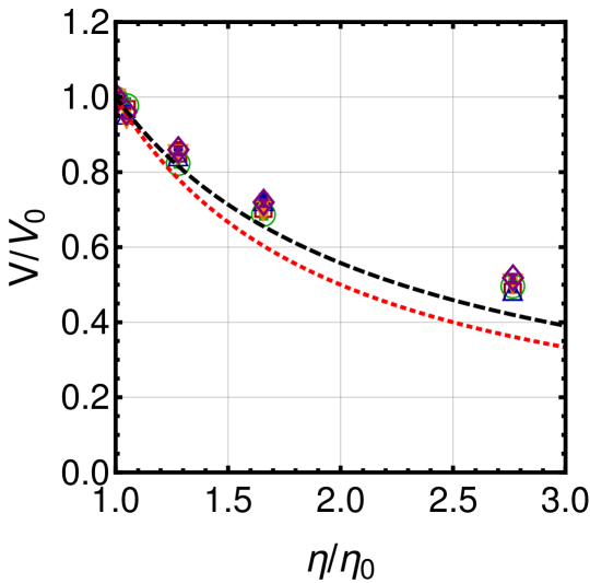
Figure 10: Velocities, $V$, of the differently-shaped colloids scaled by their respective velocities in a solution with no polymers, $V_{0}$, as a function of scaled fluid viscosity, $\eta/\eta_{0}$. The black dashed curve shows a theoretical estimate which includes the effect of a finite polymer depletion layer around the particle. The red dotted curve shows the theoretical velocities when the depletion layer is neglected. Symbol/color code as in Table 1.

The authors of Refs.[26, 27] also provide a formula for the velocity of the sphere in the presence of the depletion layer. In Fig. 10 we show how the measured velocities of the spheres, ellipsoids and rods depend on the viscosity of the fluids, and compare the numerical results to the theoretical predictions [26, 27] using a depletion layer thickness $\delta=a_{0}$ (black dashed line). Although we do not find perfect quantitative agreement with the theory, the two-fluid model matches our results much better than simply assuming that the colloid velocity is inversely proportional to the fluid viscosity (red dotted line).

4 Summary

We have performed coarse-grained hydrodynamic MPCD simulations of driven spheres, ellipsoids and rods moving in explicitly modeled polymer solutions. We first determined how the average particle velocities depend on particle shape, polymer densities, driving force and polymer type. We then measured the flow fields and local polymer density around the particles. Our main finding was that polymer-depleted regions close to the particles are responsible for an apparent tangential slip velocity. The thickness of the polymer depleted layer depends on both the density and type of the polymers. The depletion layer accounts for the measured flow fields and particle velocities, which we capture by a simple model that assumes two layers of different viscosities. We further showed that at sufficiently strong driving forces polymers become stretched and oriented perpendicular to the particle orientation in front of it, and parallel behind it.

Interestingly, there is little difference in the results for spheres, ellipsoids and rods, probably because we have chosen the same semi-minor axis $a$ for all particles. Varying $a$ will be of interest in future work. Moreover, while we performed simulations using simple polymeric fluids, it would be interesting to look for possible effects of shear thinning when using longer polymers, or elasticity if the polymers can create a large number of physical crosslinks.

References

References

- [1] E. Frey and K. Kroy, Ann. Phys. 14, 20 (2005).
- [2] F. Amblard, A. C. Maggs, B. Yurke, A. N. Pargellis, and S. Leibler, Phys. Rev. Lett. 77, 4470 (1996).
- [3] R. Metzler and J. Klafter, Phys. Rep. 339, 1 (2000).
- [4] J. Szymanski and M. Weiss, Phys. Rev. Lett. 103, 038102 (2009).
- [5] H. Guo, G. Bourret, R. B. Lennox, M. Sutton, J. L. Harden, and R. L. Leheny, Phys. Rev. Lett. 109, 055901 (2012).
- [6] F. Höfling and T. Franosch, Rep. Prog. Phys. 76, 046602 (2013).
- [7] A. M. Menzel, Phys. Rep. 554, 1 (2015).
- [8] A. Zöttl and H. Stark, J. Phys.: Condens. Matter 28, 253001 (2016).
- [9] C. Bechinger, R. Di Leonardo, H. Löwen, C. Reichhardt, G. Volpe, and G. Volpe, Rev. Mod. Phys. 88, 045006 (2016).
- [10] K. Norregard, R. Metzler, C. M. Ritter, K. Berg-Sorensen, and L. B. Oddershede, Chem. Rev. 117, 4342 (2017).
- [11] S. S. Olmsted, J. L. Padgett, A. I. Yudin, K. J. Whaley, T. R. Moench, and R. A. Cone, Biophys. J. 81, 1930 (2001).
- [12] S. K. Lai, D. E. O’Hanlon, S. Harrold, S. T. Man, Y.-Y. Wang, R. Cone, and J. Hanes, Proc. Natl. Ac. Sci. 104, 1482 (2007).
- [13] S. K. Lai, Y.-Y. Wang, and J. Hanes, Adv. Drug Del. Rev. 61, 158 (2009).
- [14] J. Kirch, A. Schneider, B. Abou, A. Hopf, U. F. Schaefer, M. Schneider, C. Schall, C. Wagner, and C.-M. Lehr, Proc. Natl. Ac. Sci. 45, 18355 (2012).
- [15] B. Button, L.-H. Cai, C. Ehre, M. Kesimer, D. B. Hill, J. K. Sheehan, R. C. Boucher, and M. Rubinstein, Science 337, 937 (2012).
- [16] M. Ernst, T. John, M. Guenther, C. Wagner, U. F. Schaefer, and C.-M. Lehr, Biophys. J. 112, 172 (2017).
- [17] Y. Cu and W. M. Saltzman, Adv. Drug Del. Rev. 61, 101 (2009).
- [18] J. T. Kalathi, U. Yamamoto, K. S. Schweizer, G. S. Grest, and S. K. Kumar, Phys. Rev. Lett. 112, 108301 (2014).
- [19] T. Ge, J. T. Kalathi, J. D. Halverson, G. S. Grest, and M. Rubinstein, Macromolecules 50, 1749 (2017).
- [20] Z. Li, Phys. Rev. E 80, 061204 (2009).
- [21] O. Lieleg and K. Ribbeck, Trends Cell Biol. 9, 543 (2011).
- [22] S. C. McBain, H. H. P. Yiu, and J. Dobson, Int. J. Nanomedicine 3, 169 (2008).
- [23] S. J. Kuhn, D. E. Hallahan, and T. D.Giorgio, Ann. Biomed. Eng. 34, 51 (2006).
- [24] C. Gutsche, F. Kremer, M. Krüger, M. Rauscher, R. Weeber, and J. Harting, J. Chem. Phys. 129, 084902 (2008).
- [25] G. H. Koenderink, S. Sacanna, D. G. A. L. Aarts, and A. P. Philipse, Phys. Rev. E 69, 021804 (2004).
- [26] R. Tuinier, J.K.G. Dhont, and T.-H. Fan, Europhys. Lett. 75, 929 (2006).
- [27] T.-H. Fan, J.K.G. Dhont, and R. Tuinier, Phys. Rev. E 75, 011803 (2007).
- [28] T. Odijk, Biophys. J. 79, 2314 (2000).
- [29] P. Illien, O. Bénichou, G. Oshanin, and R. Voituriez, Phys. Rev. Lett. 113, 030603 (2014).
- [30] N. Ter-Oganessian, B. Quinn, D. A. Pink, and A. Boulbitch, Phys. Rev. E 72, 041510 (2005).
- [31] S. H. Lee and R. Kapral, J. Chem. Phys. 121, 11163 (2004).
- [32] J. T. Padding and A. A. Louis, Phys. Rev. E 74, 031402 (2006).
- [33] A. Malevanets and J. M. Yeomans, Europhys. Lett. (EPL) 52, 231 (2000).
- [34] N. Kikuchi, A. Gent, and J. M. Yeomans, Eur. Phys. J. E 9, 63 (2002).
- [35] M. Ripoll, K. Mussawisade, R. G. Winkler and G. Gompper, Europhys. Lett. 68 106 (2004).
- [36] R.G. Winkler, K. Mussawisade, M. Ripoll and G. Gompper, J. Phys.: Condens. Matter 16 S3941 (2004).
- [37] S. H. Lee and R. Kapral, J. Chem. Phys. 124, 214901 (2006).
- [38] N. Watari, M. Makino, N. Kikuchi, R. G. Larson, and M. Doi, J. Chem. Phys. 126, 03B603 (2007).
- [39] C.-C. Huang, R. G. Winkler, G. Sutmann, and G. Gompper, Macromolecules 43, 10107 (2010).
- [40] S. Li, H. Jiang, and Z. Hou, Chinese Journal of Chemical Physics 29, 549 (2016).
- [41] A. Chen, N. Zhao and Z. Hou, Soft Matter 13, 8625 (2017).
- [42] R. Chen, R. Poling-Skutvik, A. Nikoubashman, M. P. Howard,J. C. Conrad, and J. C. Palmer, Macromolecules 51, 1865 (2018).
- [43] R. Kapral, Adv. Chem. Phys. 140, 89 (2008).
- [44] G. Gompper, T. Ihle, D. M. Kroll, and R. G. Winkler, Adv. Polym. Sci. 221, 1 (2009).
- [45] J. D. Weeks, D. Chandler, and H. C. Andersen, J. Chem. Phys. 54, 5237 (1971).
- [46] A. H. Barr, IEEE Comput. Graph. Appl. 1, 11 (1981).
- [47] A. K. Balin, A. Zöttl, J. M. Yeomans, and T. Shendruk, Phys. Rev. Fluids 2, 113102 (2017).
- [48] A. Zöttl and J. M. Yeomans, arXiv:1710.03505 (2017).
- [49] A. Zöttl and H. Stark, Eur. Phys. J. E 41, 61 (2018).
- [50] M. P. Allen and D. J. Tildesley, Computer Simulation of Liquids, (Clarendon Press, Oxford, England, 1989).
- [51] J. Hu, M. Yang, G. Gompper, and R. G. Winkler, Soft Matter 11, 7867 (2015).
- [52] S. Kim and J. S. Karrila, Microhydrodynamics - Principles and Selected Applications, (Dover Publications, Inc.,1991).
- [53] R. Piazza, Rep. Prog. Phys. 77, 056602 (2014).
- [54] E. Lauga, M. Brenner, and H. Stone, in Handbook of Experimental Fluid Dynamics, edited by J. Foss, C. Tropea, and A. Yarin (Springer, New York,2006).
- [55] P.-G. de Gennes, Scaling concepts in polymer physics, 7th ed. (Cornell University Press, London, 1979).