SPARCs for Unsourced Random Access

Abstract

Unsourced random-access (U-RA) is a type of grant-free random access with a virtually unlimited number of users, of which only a certain number $K_{a}$ are active on the same time slot. Users employ exactly the same codebook, and the task of the receiver is to decode the list of transmitted messages. We present a concatenated coding construction for U-RA on the AWGN channel, in which a sparse regression code (SPARC) is used as an inner code to create an effective outer OR-channel. Then an outer code is used to resolve the multiple-access interference in the OR-MAC. We propose a modified version of the approximate message passing (AMP) algorithm as an inner decoder and give a precise asymptotic analysis of the error probabilities of the AMP decoder and of a hypothetical optimal inner MAP decoder. This analysis shows that the concatenated construction under optimal decoding can achieve a vanishing per-user error probability in the limit of large blocklength and a large number of active users at sum-rates up to the symmetric Shannon capacity, i.e. as long as $K_{a}R<0.5\log_{2}(1+K_{a}{\sf SNR})$. This extends previous point-to-point optimality results about SPARCs to the unsourced multiuser scenario. Furthermore, we give an optimization algorithm to find the power allocation for the inner SPARC code that minimizes the ${\sf SNR}$ required to achieve a given target per-user error probability with the AMP decoder.

I Introduction

In new application scenarios of wireless networks such as Internet-of-Things (IoT), it is envisioned that a very large number of devices (referred to as users) are sending data to a common access point. Typical examples thereof include sensors for monitoring smart infrastructure or biomedical devices. This type of communication is characterized by short messages and sporadic activity. The large number of users and the sporadic nature of the transmission makes it very wasteful to allocate dedicated transmission resources to all the users. In contrast to these requirements, the traditional information theoretic treatment of the multiple-access uplink channel is focused on few users $K$, large blocklength $n$ and coordinated transmission, in the sense that each user is given an individual distinct codebook, and the $K$ users agree on which rate $K$-tuple inside the capacity region to operate [2, 3, 4]. Mathematically, this is reflected by considering the limit of infinite message- and blocklength while keeping the rate and the number of users fixed. This approach does not capture the bursty random arrival of messages in real world multiple access networks [5], which lead to the widespread success of packet based random-access models [6, 7, 8, 9]. Such models are based on simplified collision channels [10], which ignore the underlying physical communication and are thereby limited in the achievable performance [11, 12]. An alternative information theoretic route, more suited to capture the short messages of machine-type communication, was taken in recent works like [13, 14], where the number of users $K$ is taken to infinity along with the blocklength. It was shown that the information theoretic limits may be drastically different when the number of users grows together with the blocklength.

On a high level, we distinguish between grant-based and grant-free approaches. In a grant-based protocol the active users are identified and the base-station (BS) can then allocate transmission resources to the active users, while in a grant-free protocol the users transmit their data right away without awaiting the approval of the BS. For a recent overview of grant-free protocols see [15]. A novel grant-free random access paradigm, referred to as unsourced random-access (U-RA), was suggested in [14]. In U-RA each user employs the same codebook and the task of the decoder is to recover the list of transmitted messages irrespective of the identity of the users. The number of inactive users in such a model can be arbitrarily large and the performance of the system depends only on the number of active users $K_{a}$. Furthermore, a transmission protocol without the need for a subscriber identity is well suited for mass production. These features make U-RA particularly interesting for the aforementioned IoT applications.

In [14] the U-RA model for the real adder AWGN-MAC was introduced and a finite-blocklength random coding bound on the achievable energy-per-bit over noise power spectral density ($E_{b}/N_{0}$) was established. In following works several practical approaches were suggested which successively reduced the gap to the random coding achievability bound [16, 17, 18, 19]. The model has been extended to fading [20] and MIMO channels [21]. A concatenated coding approach for the U-RA problem on the real adder AWGN was proposed in [17]. The idea is to split each transmission into $L$ subslots. In each subslot the active users send a column from a common inner coding matrix, while the symbols across all subslots are chosen from a common outer tree code. We build upon the finding of [17] and its similarity to sparse regression codes (SPARCs) to give an improved inner decoder and a complete asymptotic error analysis. SPARCs were introduced in [22] as a class of channel codes for the point-to-point AWGN channel, which can achieve rates up to Shannon capacity under maximum-likelihood decoding. Later, it was shown that SPARCs can achieve capacity under approximate message passing (AMP) decoding with either power allocation [23] or spatial coupling [24, 25, 26, 27]. AMP is an iterative low-complexity algorithm for solving random linear estimation problems or generalized versions thereof [28, 29, 30]. A recent survey on SPARCs can be found in [31].

One of the appealing features of the AMP algorithm is that it is possible to analyse its asymptotic error probability, averaged over certain random matrix ensembles, through the so called state evolution (SE) equations [30, 32]. Interestingly the SE equations can also be obtained as the stationary points of the replica symmetric (RS) potential, an expression that was first calculated through the non-rigorous replica method [33, 34]. It was shown that in random linear estimation problems the stationary points of the RS potential also characterize the symbols-wise posterior distribution of the input elements and therefore also the error probability of several optimal estimators like the minimum-mean-square error (MMSE) estimator [34, 35]. The difference between the AMP and the MMSE estimate is that the MMSE estimate always corresponds to the global minimum of the RS-potential, while the AMP algorithm gets ‘stuck’ in local minima. The rate below which a local minimum appears was called the algorithmic or belief-propagation threshold in [35, 36, 25]. It was shown in [36, 37] that, despite the existence of local minima in the RS-potential, the AMP algorithm can still converge to the global minimum when used with spatially coupled matrices. Although the RS-potential was derived by (and named after) the non-rigorous replica method, it was recently proven to hold rigorously [38, 39]. The proof of [39] is more general in the sense that it includes the case where the unknown, to be estimated, vector of information symbols consists of blocks of size $2^{J}$ and each block is considered to be drawn iid from some distribution on $\mathbb{R}^{2^{J}}$.
Our main contribution in this work are as follows

• We extend the concept of sparse regression codes to the unsourced random access setting by making use of the tree code of [17].

• For the resulting inner-outer concatenated coding scheme, we introduce a matching outer channel model, analyse the achievable rates on this outer channel, and compare it to existing practical solutions.

• We propose a modified approximate message passing algorithm as an inner decoder and analyse its asymptotic error probability through its SE. We use the connections between SE and the RS formula to find the error probability of a hypothetical MAP decoder.

• We find that the error probability of the inner decoder admits a simple closed form in the limit of $K_{a},J\to\infty$ with $J=\alpha\log_{2}K_{a}$ for some $\alpha>1$. The limit was also considered in [17], motivated by the fact that $J$ is the number of bits required to encode the identity of each of up to $K_{\text{tot}}$ users if $K_{a}=K_{\text{tot}}^{1/\alpha}$. We show that the per-user error probability of the concatenated scheme with inner MAP decoding vanishes in the limit of large blocklength and infinitely many users, if the sum-rate is smaller than the symmetric Shannon capacity $0.5\log_{2}(1+K_{a}{\sf SNR})$. This shows that an unsourced random access scheme can, even with no coordination between users, achieve the same symmetric rates as a non-unsourced scheme.

• Using the results from the asymptotic analysis we identify parameter regions where the AMP decoder can achieve the same error probability as the MAP decoder. In parameter regions where there is a gap between the achievable error probability of the AMP and the MAP decoder we propose a method for finding an optimal power allocation that is able to improve the performance of the AMP decoder significantly.

• We provide finite-length simulations to show the efficiency of the proposed coding scheme and the accuracy of the analytical predictions.

The paper is organized as follows. In Section II we describe the channel model. In Section III we introduce the concatenated coding scheme. In Section IV we introduce the inner AMP decoder and the optimal, but uncomputable, MAP decoder and analyse their asymptotic error probabilities. In Section V we analyse the quantization step, which is necessary for a binary-input outer decoder. In Section VI we formulate the outer channel and give converse and achievability results. In Section VII we analyse the concatenated code. In Section VIII we give an algorithm to optimize the power allocation and in Section IX we introduce a low-complexity approximation of the suggested AMP algorithm. In Section X we give finite-length simulations and compare them to the analytical results.

II Channel Model

Let $K_{a}$ denote the number of active users, $n$ the number of available channel uses and $B=nR$ the size of a message in bits. The spectral efficiency is given by $\mu=K_{a}R$. The channel model used is

$${\bf y}=\sum_{i=1}^{K_{\text{tot}}}q_{i}{\bf x}_{i}+{\bf z},$$ (1)

where each ${\bf x}_{i}\in\mathcal{C}\subset\mathbb{R}^{n}$ is taken from a common codebook $\mathcal{C}$ and $q_{i}\in\{0,1\}$ are binary variables indicating whether a user is active. The number of active users is denoted as $K_{a}=\sum_{i=1}^{K_{\text{tot}}}q_{i}$. The codewords are assumed to be normalized as $\|{\bf x}_{i}\|_{2}^{2}=nP$ for a given energy-per-symbol $P$, and the noise vector ${\bf z}$ is Gaussian iid $z_{i}\sim\mathcal{N}(0,N_{0}/2)$, such that ${\sf SNR}=2P/N_{0}$ denotes the per-user ${\sf SNR}$. All the active users pick one of the $2^{B}$ codewords from $\mathcal{C}$, based on their message $W_{k}\in[1:2^{B}]$. The decoder of the system produces a list $g({\bf y})$ of at most $K_{a}$ messages. An error is declared if one of the transmitted messages is missing in the output list $g({\bf y})$ and we define the per-user probability of error as:

$$P_{e}=\frac{1}{K_{a}}\sum_{k=1}^{K_{a}}\mathbb{P}(W_{k}\notin g({\bf y})).$$ (2)

Note that the error is independent of the user identities in general and especially independent of the inactive users. The performance of the system is measured in terms of the required $E_{b}/N_{0}:=P/(RN_{0})$ for a target $P_{e}$ and the described coding construction is called reliable if $P_{e}\to 0$ as $n\to\infty$.

III Concatenated Coding

In this work we focus on a special type of codebook, where each transmitted codeword is created in the following way: First, the $B$-bit message $W_{k}$ of user $k$ is mapped to an $LJ$-bit codeword from some common outer codebook. Then each of the $J$-bit sub-sequences is mapped to an index $i_{k}(l)\in[1:2^{J}]$ for $l=[1:L]$ and $k=[1:K_{a}]$. The inner codebook is based on a set of $L$ coding matrices ${\bf A}_{l}\in\mathbb{R}^{n\times 2^{J}}$. Let ${\bf a}^{(l)}_{i}$ with $i=[1:2^{J}]$ denote the columns of ${\bf A}_{l}$. The inner codeword of user $k$ corresponding to the sequence of indices $i_{k}(1),...,i_{k}(L)$ is then created as

$${\bf x}_{k}=\sum_{l=1}^{L}\sqrt{P_{l}}{\bf a}^{(l)}_{i_{k}(l)}.$$ (3)

The columns ${\bf a}^{(l)}_{i}$ of ${\bf A}_{l}$ are assumed to be zero mean and scaled such that $\|{\bf a}^{(l)}_{i}\|_{2}^{2}=1$ and the power coefficients $P_{l}$ are chosen such that $\mathbb{E}[\|{\bf x}_{k}\|_{2}^{2}]\leq nP$ where the expectation is taken over all choices of indices $(i_{k}(1),...,i_{k}(L))$. The above encoding model can be written in matrix form as

$${\bf y}=\sum_{k=1}^{K_{a}}{\bf A}{\bf m}_{k}+{\bf z}={\bf A}\left(\sum_{k=1}^{K_{a}}{\bf m}_{k}\right)+{\bf z}.$$ (4)

where ${\bf A}=({\bf A}_{1}|...|{\bf A}_{L})$ and ${\bf m}_{k}\in\mathbb{R}^{L2^{J}}$ is a non-negative vector satisfying $m_{k,(l-1)2^{J}+i_{k}(l)}=\sqrt{P_{l}}$ and zero otherwise, for all $l=[1:L]$. Let $\hbox{\boldmath$\theta$}=\sum_{k=1}^{K_{a}}{\bf m}_{k}$ and let ${\bf s}$ denote the support of $\theta$ with multiplicity, such that $\hbox{\boldmath$\theta$}=\left(\sqrt{P_{1}}{\bf s}^{1}|...|\sqrt{P_{L}}{\bf s}^{L}\right)^{\top}$. That is, the components of ${\bf s}^{l}$ indicate how many active users have chosen a specific column of ${\bf A}_{l}$. We refer to $\sqrt{P_{l}}{\bf s}^{l}$ as the $l$-th section of $\theta$. The linear structure allows to write the channel (4) as a concatenation of the inner point-to-point channel $\hbox{\boldmath$\theta$}\to{\bf A}\hbox{\boldmath$\theta$}+{\bf z}$ and the outer binary input adder MAC $({\bf m}_{1},...,{\bf m}_{K_{a}})\to{\bf s}$. We will refer to those as the inner and outer channel, the corresponding encoder and decoder will be referred to as inner and outer encoder/decoder and the aggregated system of inner and outer encoder/decoder as the concatenated system. The per-user inner rate in terms of bits per channel use (c.u.) is given by $R_{\text{in}}:=LJ/n$ and the outer rate is given by $R_{\text{out}}=B/LJ$. For the sake of the analysis we shall consider a random ensemble of codes where the matrices ${\bf A}_{l}$ are generated with i.i.d. Gaussian components $\sim\mathcal{N}(0,1/n)$ and the outer encoded indices $i_{k}(l)$ are distributed uniformly and independently over $[1:2^{J}]$. Furthermore, we assume that the power coefficients are uniformly $P_{l}\equiv nP/L$, such that the power constraint $\mathbb{E}[\|{\bf x}_{k}\|_{2}^{2}]\leq nP$ is fulfilled on average over the code ensemble. The uniform power allocation will be relaxed in Section VIII, where we will consider a non-uniform power allocation.

IV Inner Channel

In this section we focus on the inner decoding problem of recovering ${\bf s}$ from

$${\bf y}={\bf A}\hbox{\boldmath$\theta$}+{\bf z}=\sqrt{\hat{P}}{\bf A}{\bf s}+{\bf z}$$ (5)

where $\hat{P}=nP/L$. Let $k_{i}\in[0:K_{a}]$ for $i\in[1:2^{J}]$ be non-negative integers. The probability of observing a specific ${\bf s}^{l}$ is given by:

$$p\left({\bf s}^{l}=(k_{1},...,k_{2^{J}})^{\top}\right)=2^{-K_{a}J}\frac{K_{a}!}{k_{1}!\cdots k_{2^{J}}!}$$ (6)

if $\sum_{i=1}^{2^{J}}k_{i}=K_{a}$ and zero otherwise. This is a multinomial distribution with uniform event probabilities. The marginals of such a distribution are known to be Binomial, i.e.:

$$p_{k}:=\mathbb{P}(s^{l}_{i}=k)={K_{a}\choose k}2^{-kJ}(1-2^{-J})^{K_{a}-k}$$ (7)

and specifically, the probability of observing a zero is:

$$p_{0}:=\mathbb{P}(s^{l}_{i}=0)=(1-2^{-J})^{K_{a}}.$$ (8)

We define two estimators for ${\bf s}$. The first is a variant of the approximate message passing (AMP) algorithm, which we will refer to as AMP-estimator. An estimate of ${\bf s}$ is obtained by iterating the following equations:

$$\begin{split}\hbox{\boldmath$\theta$}^{t+1}&=f_{t}({\bf A}^{\top}{\bf z}^{t}+\hbox{\boldmath$\theta$}^{t})\\ {\bf z}^{t+1}&={\bf y}-{\bf A}\hbox{\boldmath$\theta$}^{t+1}+\frac{2^{J}L}{n}{\bf z}^{t}\langle f^{\prime}_{t}({\bf A}^{\top}{\bf z}^{t}+\hbox{\boldmath$\theta$}^{t})\rangle\end{split}$$ (9)

where the function $f_{t}:\mathbb{R}^{2^{J}L}\to\mathbb{R}^{2^{J}L}$ is defined componentwise $f_{t}({\bf x})=(f_{t,1}(x_{1}),...,f_{t,2^{J}L}(x_{2^{J}L}))^{\top}$ and each component is given by

$$f_{t,i}(x)=\frac{\sqrt{\hat{P}}}{Z(x)}\sum_{k=0}^{K_{a}}p_{k}k\exp\left(\frac{1}{2\tau_{t}^{2}}\left(x-k\sqrt{\hat{P}}\right)^{2}\right)$$ (10)

with $\tau^{2}_{t}=\|{\bf z}^{t}\|_{2}^{2}/n$, $p_{0}$ as in (8) and

$$Z(x)=\sum_{k=0}^{K_{a}}p_{k}\exp\left(\frac{1}{2\tau_{t}^{2}}\left(x-k\sqrt{\hat{P}}\right)^{2}\right).$$ (11)

$\langle{\bf x}\rangle=(\sum_{i=1}^{N}x_{i})/N$ in (9) denotes the arithmetic mean of a vector, $f^{\prime}_{t}$ denotes the componentwise derivative of $f_{t}$ and ${\bf z}^{0}=\mathbf{0}$ is chosen as the initial value. After the equations (9) are iterated for some fixed number of iterations $T_{\text{max}}$, a final estimate of ${\bf s}$ is obtained by quantizing $\hbox{\boldmath$\theta$}^{T_{\text{max}}}$ to the nearest integer multiple of $\sqrt{\hat{P}}$ and dividing by $\sqrt{\hat{P}}$. Note, that each of the functions $f_{t,i}$ in (10) is chosen as the posterior-mean estimator (PME) of the component $\theta_{i}$ in a scalar Gaussian channel with noise variance $\tau_{t}^{2}$. This is justified by the remarkable property of the AMP algorithm that the terms ${\bf A}^{\top}{\bf z}^{t}+\hbox{\boldmath$\theta$}^{t}$ are distributed approximately like $\mathcal{N}(\hbox{\boldmath$\theta$},\tau_{t}^{2}{\bf I})$, i.e. like the true signal in iid Gaussian noise [30, 32].

The second estimator that we analyse is the symbol-by-symbol maximum-a-posteriori (SBS-MAP) estimator of ${\bf s}$

$$\hat{s}^{l}_{i}=\operatorname*{arg\,max}_{s\in[0:K_{a}]}\mathbb{P}(s^{l}_{i}=s|{\bf y},{\bf A}),$$ (12)

which minimizes the SBS error probability $\mathbb{P}(\hat{s}^{l}_{i}\neq s^{l}_{i})$ but is infeasible to compute in practice. Let

$$P_{e}^{\text{in}}=\frac{1}{L2^{J}}\sum_{l=1}^{L}\sum_{j=1}^{2^{J}}\mathbb{P}(\hat{s}^{l}_{j}\neq s^{l}_{j})$$ (13)

denote the inner per-user SBS error rate for some symbol-wise estimator $\hat{s}^{l}_{j}$, and let $P_{e}^{\text{MAP}}$ and $P_{e}^{\text{AMP}}$ denote the corresponding inner error rates of the MAP and the AMP estimator respectively.

IV-A Asymptotic Error Analysis

The error analysis is based on the self-averaging property of the random linear recovery problem (5) in the asymptotic limit $L,n\to\infty$ with a fixed $J$ and fixed $R_{\text{in}}$. That is, although ${\bf A},{\bf s}$ and ${\bf z}$ are random variables, the error probability of both mentioned estimators converges sharply to its average value. The convergence behavior is fully characterized by the external parameters $J,R_{\text{in}},{\sf SNR}$ and $K_{a}$. It is known that the asymptotic estimation error of the AMP algorithm can be analysed by the so called state evolution (SE) equations [30].

Theorem 1.

In the limit $n,L\to\infty$ for fixed $J$ and fixed $R_{\text{in}}$ the mean-square-error (MSE) of the AMP estimate (9) converges to the MSE of estimating $s$ in the scalar Gaussian channel

$$r=\sqrt{\eta\hat{P}}s+z$$ (14)

where $s$ is distributed according to the binomial distribution $p(s=k)$ specified in (7), i.e. the marginal distribution of a single section of ${\bf s}$, and $z\sim\mathcal{N}(0,1)$ is independent of $s$. The factor $\eta\geq 0$ is given as the smallest non-negative solution of

$$\frac{\mathrm{d}}{\mathrm{d}\eta}i^{\text{RS}}_{\text{AMP}}(\eta)=0$$ (15)

where $i^{\text{RS}}_{\text{AMP}}(\eta)$ is given by

$$i^{\text{RS}}_{\text{AMP}}(\eta)=2^{J}I(\eta\hat{P})+\frac{2^{J}}{2\beta}[(\eta-1)\log_{2}(e)-\log_{2}(\eta)]$$ (16)

$I(\eta\hat{P})$ denotes the mutual information between $r$ and $s$ in the scalar Gaussian channel (14). $\hfill\square$

Proof.

The theorem is merely a restatement of the SE result in [30] which states that the MSE of $\hbox{\boldmath$\theta$}^{t}$ can be described asymptotically by a scalar Gaussian channel where the effective noise variance follows the recursion

$$\tau^{2}_{t+1}=1+\beta\hat{P}\mathbb{E}[(s-f_{t}(\hat{P}s+\tau_{t}^{2}z))^{2}]$$ (17)

with $\tau_{0}^{2}=\|{\bf y}\|_{2}^{2}/n$ and $s,z$ jointly distributed as in (14). It is well known that in general the minimum-mean-square error (MMSE) can be achieved by the PME $\mathbb{E}[s|y]$. Since $f_{t}$ was chosen precisely as the PME of $\sqrt{\hat{P}}s$ in a scalar Gaussian channel of the form (14) with $\eta=1/\tau_{t}^{2}$, it holds that

$$\mathbb{E}[(s-f_{t}(\hat{P}s+\tau_{t}^{2}z))^{2}]=\text{mmse}(\eta\hat{P}),$$ (18)

where we introduce the MMSE function $\text{mmse}(\eta\hat{P})=\mathbb{E}[(s-\mathbb{E}[s|y])^{2}]$ in a Gaussian channel (14). Since the recursion starts at a high noise (low $\eta$) point and because $\text{mmse}(\eta\hat{P})$ is monotonically decreasing in $\eta$ the point of convergence is given by the smallest $\eta$ for which

$$\eta^{-1}=1+\beta\hat{P}\text{mmse}(\eta\hat{P})$$ (19)

holds. Setting the derivative of (16) with respect to $\eta$ to zero shows that (19) is precisely the condition for a stationary point. This can be seen using the I-MMSE theorem [40], which states that in a Gaussian additive noise channel it holds that:

$$\frac{1}{\log_{2}(e)}\frac{\mathrm{d}}{\mathrm{d}\eta}I(\eta\hat{P})=\frac{\hat{P}}{2}\text{mmse}(\eta\hat{P})$$ (20)

∎

The mutual information in (16) is bounded by the entropy of the input distribution for $\eta\to 0$ and so $\lim_{\eta\to 0}i^{RS}(\eta)=\infty$. Furthermore, (16) is continuously differentiable and therefore the smallest stationary point, i.e. the smallest $\eta$ for which $\mathrm{d}i^{\text{RS}}(\eta)/\mathrm{d}\eta=0$, is necessarily either a local minimum or a saddle point but never a local maximum. Note that although the assumed distribution on ${\bf s}$ is not iid the AMP algorithm in (9) uses a separable denoiser. In this case the SE result of [30] does not require ${\bf s}$ to be iid, but only that its empirical marginal distributions converge to some limit, which is required for the calculation of the SE. In fact, the presented AMP algorithm (9) is not optimal since it does not make full use of the distribution of ${\bf s}$, i.e. it ignores the correlation among different components of ${\bf s}$ within a section. The optimal AMP algorithm would use the vector PME of ${\bf s}$ in the following Gaussian vector channel as a denoiser:

$${\bf r}^{l}=\sqrt{\eta\hat{P}}{\bf s}^{l}+{\bf z}^{l}$$ (21)

where ${\bf s}^{l}\in\mathbb{R}^{2^{J}}$ is distributed according to the vector distribution $p({\bf s}^{l})$, specified in (6), the distribution of a single section of ${\bf s}$, and ${\bf z}^{l}\in\mathbb{R}^{2^{J}}$ is Gaussian iid with $\mathcal{N}(0,1)$ components, independent of ${\bf s}^{l}$. The vector PME can be expressed as follows

$$f_{t,l}^{\text{opt}}=\frac{1}{Z({\bf r}^{l})}\sum_{{\bf s}^{l}}{\bf s}^{l}\exp\left(-\frac{1}{2}\left\|{\bf r}^{l}-\sqrt{\eta\hat{P}}{\bf s}^{l}\right\|^{2}_{2}\right)p({\bf s}^{l}),$$ (22)

where $\sum_{{\bf s}^{l}}$ denotes the sum over all possible configurations within one section and $Z({\bf r}^{l})$ is a normalisation factor. Note, that the number of possible configurations of ${\bf s}_{l}$, and therefore the number of terms in the sum $\sum_{{\bf s}^{l}}$, grows exponentially in $J$ and $K_{a}$ which makes the direct computation of the vector PME infeasible. Nonetheless, according to [32], the MSE of this infeasible version of AMP can be tracked in the same way as in Theorem 1 but with the vector channel (21) instead of the scalar channel and $\eta\geq 0$ is given as the smallest stationary point of the potential

$$i^{\text{RS}}(\eta)=I_{2^{J}}(\eta\hat{P})+\frac{2^{J}}{2\beta}[(\eta-1)\log_{2}(e)-\log_{2}(\eta)]$$ (23)

where $I_{2^{J}}(\eta\hat{P})$ denotes the mutual information between ${\bf r}^{l}$ and ${\bf s}^{l}$ in the Gaussian vector channel (21) and $\beta=2^{J}L/n=R_{\text{in}}2^{J}/J$ is the aspect ratio of the matrix ${\bf A}$ in (5). Note, that for $J=0$, i.e. blocks of size one, (23) coincides (16).

An integral part of the proof of the SE equations in [30, 32] is that the intermediate terms ${\bf A}^{\top}{\bf z}^{t}+\hbox{\boldmath$\theta$}^{t}$, appearing in (9), are indeed asymptotically distributed as in the decoupled Gaussian channel (21). Therefore, the error statistics of any estimator that is applied to ${\bf A}^{\top}{\bf z}^{\infty}+\hbox{\boldmath$\theta$}^{\infty}$ after convergence ($t\to\infty$) can be analysed by studying the same estimator on the Gaussian channel (21) at the appropriate channel strength $\eta\hat{P}$.

A crucial point is that the asymptotic AMP performance is given by the smallest stationary point of the potential function. In particular, the MSE of AMP with the optimal vector PME (22) is described by the smallest stationary point of (23), while the MSE of AMP with the scalar PME (10) is described by the smallest stationary point of (16). Nonetheless, the potential functions also contains information about the performance of the optimal MMSE estimate $\hat{{\bf s}}=\mathbb{E}[{\bf s}|{\bf A},{\bf y}]$ [41]. Specifically, the asymptotic MMSE is given by the MSE of the PME of ${\bf s}$ in the Gaussian vector channel (21), similar to the analysis of AMP with the vector PME (22), but the effective channel strength $\eta$ is now the global minimizer of (23). We illustrate the used terminology in Figure 1. Note, that it is possible that the smallest stationary point and the global minimum coincide. In that case the AMP estimate coincides with the MMSE estimate.

Figure 1: Illustration of the RS-potential

For ${\bf s}$ with iid components, i.e. the special case $J=0$ where (23) reduces to (16), this connection was first discovered, using the non-rigorous replica method, in [33] for binary iid signals ${\bf s}$ and generalized to arbitrary iid ${\bf s}$ in [34, 29]. For this reason, the potential function (16) was termed the replica symmetric (RS) potential. This heuristic discovery was later confirmed rigorously in [38, 39]. The proof in [39, Ch. 4] is based on an adaptive interpolation approach and includes the case of block iid signals which are shown to be described by the global minimizer of (23).

Even in the iid signal case, the original results obtained by the replica method were slightly stronger then the rigorized versions in [38, 39, 41]. Specifically, they included the so called decoupling property [33, 34, 35], which informally states that, in the case of an iid prior, the conditional posterior distribution of ${\bf s}$ in the model (5) indeed behaves like the conditional posterior distribution induced by the scalar Gaussian channel (14). Motivated by the similarity of the RS potentials in the iid and in the block iid cases, respectively in (16) and (23), we conjecture that the decoupling principle holds (subject to the validity of the replica-based analysis) also for the block iid case, when the length of the blocks $2^{J}$ is constant with $n$ and $L$ . This is summarized in the following

Claim 1 (Decoupling Property).

For an arbitrary section index $l$ let ${\bf s}^{l}_{p}$ be a sample from the marginal posterior distribution $p_{{\bf s}^{l}|{\bf y},{\bf A}}$ where ${\bf y}$ is created according to model (5) and ${\bf s}^{l}_{0}$ being distributed according to the prior distribution of one section (6). We say that the decoupling property holds in some specified limit if the joint distribution of $({\bf s}^{l}_{0},{\bf s}^{l}_{p})$ converges to the joint distribution of $({\bf s}^{l}_{0},{\bf s}^{l})$ defined as follows. ${\bf s}^{l}_{0}$ is again distributed according to the prior of a single section while, conditional on ${\bf s}^{l}_{0}$, ${\bf s}^{l}$ is distributed according to the posterior distribution $p_{{\bf s}^{l}|{\bf r}^{l}}$ evaluated at the output of a Gaussian vector channel ${\bf r}^{l}=\sqrt{\eta\hat{P}}{\bf s}^{l}_{0}+{\bf z}^{l}$ with input ${\bf s}^{l}_{0}$. The factor $\eta\geq 0$ is given as the global minimizer of (23).

Remark 1.

The decoupling property implies that the error statistics of every estimator that is based purely on the marginal posterior distribution, including the SBS-MAP estimator, is asymptotically given by the error statistic of the same estimator but with the true posterior distribution replaced by a posterior distribution in a degraded Gaussian channel, where the degradation factor $\eta$ is given as the solution of the minimisation of (23). Therefore, asymptotically, once $\eta$ has been determined, the error of the SBS-MAP estimator can be computed as the error of the estimator $\hat{s}_{i}=\operatorname*{arg\,max}\mathbb{P}(s^{l}_{i}=s|{\bf r}^{l})$ in the channel (21). Claim 1 is supported by several reasons:

1. It was proven in [39, Ch. 4] that the mutual information between ${\bf s}$ and ${\bf y}$ in (5) converges to the RS potential (23). Through a limiting argument together with the I-MMSE theorem it is possible to conclude the convergence of the posterior-mean estimation error of ${\bf s}$ from (5) to the MMSE in the Gaussian vector channel [41, Corollary 7].

2. The replica-based proof of the scalar decoupling property in [34] consists of two steps. First it is shown that, subject to the validity of the replica analysis, the mutual information $I({\bf y};{\bf s})$ in (5) converges to (14). Then it is shown that all the moments of the joint distribution of $({\bf s}^{l}_{0},{\bf s}^{l})$ converge for an arbitrary index $l$ to the joint distribution of input and posterior output in a degraded Gaussian channel. The second step is obtained by essentially repeating the same calculation as in the first step.

3. In [33] it was argued that the mutual information is equivalent to the cumulant generating function and as such it contains the information about all the moments of the input-output distribution. Therefore the convergence of the mutual information would imply the decoupling property. Nonetheless, it is non-trivial to confirm such a claim in the given setting.

4. There is an strong connection between the SE of AMP and the replica method. As mentioned, the potential (23) also describes the performance of the optimal, computationally infeasible, AMP algorithm. The SE of AMP though has been proven rigorously [32], even for the case of block iid input distributions, and it is an integral part of the proof of the SE that the intermediate terms ${\bf A}^{\top}{\bf z}+\hbox{\boldmath$\theta$}^{t}$, appearing in (9), are asymptotically distributed as in the decoupled Gaussian channel (21). The major role that SE plays in the rigorous proof of the RS-potential in [41] leads us to believe that the decoupling property should also translate.

Nevertheless, the decoupling property, as stated here, is not supported by rigorous proofs in the current literature, Showing the decoupling property for block iid signals (wether via replica analysis or in a fully rigorous way) remains an interesting open problem for future work.

In the remaining chapter we give a mathematical analysis of the vector-channel based potential (23) and the scalar-channel based potential (16) and show that the componentwise PME in (10) is the best componentwise approximation of the vector PME and furthermore, in the typical sparse setting, i.e. $K_{a}\ll 2^{J}$, the difference between the minima of the two potential functions (23) and (16) is negligibly small and therefore the global minimizer of the potential (16) can be used to approximate the global minimizer of (23). This means that the error probability of both the presented AMP estimator and, through the decoupling property, the SBS-MAP estimator can be characterized by the local and global minimizers of the potential function (16) based in the mutual information in a scalar Gaussian channel. The connection between (16) and (23) is made precise in the following theorem:

Theorem 2.

Let $\eta_{\text{opt}}$ be the global minimizer of (23) and let $\tilde{\eta}_{\text{opt}}$ be the global minimizer of (16) then $\eta_{\text{opt}}>\tilde{\eta}_{\text{opt}}$ and

$$\eta_{\text{opt}}-\tilde{\eta}_{\text{opt}}=\mathcal{O}\left(\frac{R_{\text{in}}\log K_{a}}{\sqrt{J}}\right)$$ (24)

$\hfill\square$

Proof.

Analogous to (19) the optimality condition for $\eta_{\text{opt}}$ can be found by setting the derivative of (23) to zero and using the I-MMSE theorem for a Gaussian vector channel. This gives the condition

$$\eta^{-1}=1+\beta\hat{P}\frac{\text{mmse}_{2^{J}}(\eta\hat{P})}{2^{J}}$$ (25)

where $\text{mmse}_{2^{J}}(\eta\hat{P})$ is the MMSE of estimating ${\bf s}^{l}$ in the Gaussian vector channel (21). Let us introduce the mismatched MSE function. For an arbitrary probability distribution $q:[0:K_{a}]^{2^{J}}\to[0,1]$ we define

$$\text{mse}_{q}(t)=\mathbb{E}\|{\bf s}-\hat{{\bf s}}_{q}(\sqrt{t}{\bf s}+{\bf Z},t)\|_{2}^{2}$$ (26)

with

$$\hat{{\bf s}}_{q}({\bf r},t)=\sum_{{\bf s}\in[0:K_{a}]^{2^{J}}}{\bf s}\frac{\exp(-\|{\bf r}-\sqrt{t}{\bf s}\|_{2}^{2}/2)q({\bf s})}{\sum_{{\bf s}^{\prime}}\exp(-\|{\bf r}-\sqrt{t}{\bf s}^{\prime}\|_{2}^{2}/2)q({\bf s}^{\prime})}$$ (27)

The expression in (26) is the MSE of a (mismatched) PME in a Gaussian vector channel of the form (21) with respect to some prior distribution $q({\bf s})$, which may differ form the true prior $p_{\bf s}({\bf s})$. It is clear that from the minimality of the MMSE function that $\text{mmse}_{2^{J}}(t)\leq\text{mse}_{q}(t)$ for all $t$ with equality if $q({\bf s})=p_{\bf s}({\bf s})$. This means, that calculating the fixed-point of (25), with $\text{mmse}_{2^{J}}(t)$ replaced by $\text{mse}_{q}(t)$ for any choice of $q({\bf s})$ gives an upper bound on $\eta_{\text{opt}}$. The $L^{1}$-distance between the functions $\text{mmse}_{2^{J}}(t)$ and $\text{mse}_{q}(t)$ is quantified by the following result from [42]

$$\begin{split}&\frac{1}{2}\|\text{mse}_{q}-\text{mmse}_{2^{J}}\|_{L^{1}}\\ &=\frac{1}{2}\int_{0}^{\infty}[\text{mse}_{q}(t)-\text{mmse}_{2^{J}}(t)]\mathrm{d}t=D(p_{\bf s}\ \|\ q).\end{split}$$ (28)

where $D(p_{\bf s}\ \|\ q)$ denotes the KL-divergence between the distributions $p_{\bf s}$ and $q$. We focus on product distributions of the form $q({\bf s})=\prod_{i=1}^{2^{J}}q_{i}(s_{i})$, since for such distributions the vector MSE function (26) becomes the sum of scalar MSE functions, which are easy to calculate. Moreover, a simple calculation in Appendix A shows that the $L^{1}$ distance (28) is minimized by the product distribution whose factors $q_{i}$ match the marginals of $p_{\bf s}$. We prove in Appendix B that the KL-divergence between the multinomial distribution $p_{\bf s}$ and the product distribution of its marginals satisfies

$$D\left(p_{\bf s}\ \middle\|\ \prod_{i=1}^{2^{J}}p_{i}(s_{i})\right)=\mathcal{O}(\log K_{a})$$ (29)

By substituting $\eta\hat{P}=t$ we get from (28):

$$\begin{split}&\int_{0}^{1}\text{mse}_{q}(\eta\hat{P})-\text{mmse}_{2^{J}}(\eta\hat{P})\mathrm{d}\eta\\ &=\frac{1}{\hat{P}}\int_{0}^{\hat{P}}\text{mse}_{q}(t)-\text{mmse}_{2^{J}}(t)\mathrm{d}t\\ &<\frac{D\left(p_{\bf s}\ \middle\|\ \prod_{i=1}^{2^{J}}p_{i}(s_{i})\right)}{\hat{P}}\end{split}$$ (30)

Furthermore, since all marginals of $p_{\bf s}$ are identical and given by the binomial distribution, the mismatched MSE function of $q({\bf s})=\prod p_{i}(s_{i})$ takes the form

$$\text{mse}_{q}(t)=2^{J}\text{mmse}(t),$$ (31)

where $\text{mmse}(t)$ is the MMSE function in the scalar Gaussian channel (14) that appears in (19). So it follows from (28) and (29) that as a function of $\eta\in[0,1]$

$$\left\|\text{mmse}(\cdot\hat{P})-\frac{\text{mmse}_{2^{J}}(\cdot\hat{P})}{2^{J}}\right\|_{L^{1}}=\mathcal{O}\left(\frac{\log K_{a}}{2^{J}\hat{P}}\right)$$ (32)

Therefore, with $J\to\infty$, the difference between the per-component vector MMSE function in (25) and the scalar MMSE function in (19) converges exponentially fast in $L^{1}$ norm to zero. We show in Appendix C that exponentially fast convergence in $L^{1}$-norm implies exponentially fast pointwise convergence everywhere except on a set of arbitrary small measure.

The right-hand sides (RHSs) of (25) and (19) are multiplied by $\beta\hat{P}$. With the scaling conditions in Theorem 1 $\beta=R_{\text{in}}2^{J}/J$. Therefore, the difference between the RHS of (25) and (19) converges pointwise to zero with rate $\mathcal{O}(R_{\text{in}}\log K_{a}/(\delta\sqrt{J}))$ everywhere except on a set of measure $\mathcal{O}(\delta J^{-1/2})$. Since MMSE functions of Gaussian channels are non-increasing, by a well known theorem in real analysis, their pointwise convergence implies uniform convergence in all continuity points of the limit functions. Later, we will show that the common limit function of the mmse functions is continuous on two disjoint intervals divided by a single discontinuity point. Therefore, since uniform convergence preserves continuity, the pointwise convergence holds for all $\eta$ except for a single point. We have established that the difference of the right hand sides of the stationary point equations (19) and (25) converges pointwise to zero. Due to the smoothness of the MMSE functions [43, Proposition 7] the convergence carries over to the solutions of the (19) and (25) if $\eta_{\text{opt}}$ and $\tilde{\eta}_{\text{opt}}$ are away from the discontinuity point of the limiting function, which will follow later from Theorem 4. This concludes the proof of (24). ∎

Theorem 2 allows to calculate the minima of the potential (23) by solving the scalar fixed point equation (19) numerically. It guarantees that the error will be small, since typically $2^{J}$ is much larger than $K_{a}$. Nonetheless, the MMSE function in equation (19) can be further simplified if $J$ grows large. That is because the coefficients $p_{k}$ defined in (7), which can be expressed as

$$p_{k}=p_{0}\frac{{K_{a}\choose k}}{(2^{J}-1)^{k}}$$ (33)

decay exponentially with $kJ$. This suggests that for large $J$ we can drop all $p_{k}$ with $k\geq 2$:

Theorem 3.

Let $\text{mmse}_{\text{OR}}(t)$ be the MMSE function of estimating the binary variable $s_{\text{OR}}\in\{0,1\}$ in the scalar Gaussian channel

$$r=\sqrt{t}s_{\text{OR}}+z$$ (34)

where $p(s_{\text{OR}}=0)=p_{0}$ and $p(s_{\text{OR}}=1)=1-p_{0}$ and $z\sim\mathcal{N}(0,1)$ independent of $s_{\text{OR}}$. Then $\text{mmse}_{\text{OR}}(t)\geq\text{mmse}(t)$ for all $t>0$ and

$$\text{mmse}_{\text{OR}}(t)-\text{mmse}(t)=\mathcal{O}\left(\frac{K_{a}^{2}}{2^{2J}}\right)$$ (35)

$\hfill\square$

Proof.

See Appendix D. ∎

We choose the nomenclature OR in $\text{mmse}_{\text{OR}}$ because the distribution of $s_{\text{OR}}$ arises as the marginal distribution of ${\bf s}$ if we assume that it is not the sum of the individual messages ${\bf m}_{k}$ but the OR-sum:

$${\bf s}=\bigvee_{k=1}^{K_{a}}{\bf m}_{k}$$ (36)

Furthermore, let $I_{\text{OR}}(t)$ be the input-output mutual information in the channel (34) and

$$i^{\text{RS}}_{J,\text{OR}}(\eta)=I_{\text{OR}}(\eta\hat{P})+\frac{1}{2\beta}[(\eta-1)\log_{2}(e)-\log_{2}(\eta)]$$ (37)

the corresponding RS-potential. A consequence of Theorems 2 and 3 is that we can use (37) to find both the global minimizer of (23) and the local minimizer of (16).

Corollary 1.

Let $\eta_{\text{opt}}$ be the global minimizer of (23), let $\tilde{\eta}_{\text{opt}}^{\text{OR}}$ be the global minimizer of (37), let $\eta_{\text{alg}}$ be the smallest local minimizer of (16) and let $\tilde{\eta}^{\text{OR}}_{\text{alg}}$ be the smallest local minimizer of (37), then $\eta_{\text{opt}}>\tilde{\eta}_{\text{opt}}^{\text{OR}}$

$$\eta_{\text{opt}}-\tilde{\eta}_{\text{opt}}^{\text{OR}}=\mathcal{O}\left(\frac{R_{\text{in}}\log K_{a}}{\sqrt{J}}\right)$$ (38)

Furthermore, if $\eta_{\text{opt}}\neq\eta_{\text{alg}}$ then $\eta_{\text{alg}}>\tilde{\eta}_{\text{alg}}^{\text{OR}}$ and:

$$\eta_{\text{alg}}-\tilde{\eta}_{\text{alg}}^{\text{OR}}=\mathcal{O}\left(\frac{R_{\text{in}}\log K_{a}}{\sqrt{J}}\right)$$ (39)

$\hfill\square$

Note that we have only shown that the difference of the MMSE functions in the channels (21) and (34) converges to zero as $J\to\infty$. This shows that those functions converge to the same limiting function. The derivation of this limiting function itself is the subject of the following section.

IV-B The $J\to\infty$ limit

The problem with the numerical evaluation of the stationary points of (16), even when using Theorem 3, is that $2^{-J}$ is very small. We were able to evaluate the minima of (16) only up to around $J=60$. So even though (35) guarantees that the common $J\to\infty$ limit of the two MMSE functions in the channels (34) and (21) exists, it is not obvious how to calculate it numerically. To solve these problems we calculate the limit of (37) analytically in a regime where both $K_{a}$ and $J$ go to infinity with a fixed ratio $\alpha:=J/\log_{2}K_{a}$ for some $\alpha>1$. The parameter $\alpha$ determines the sparsity in the vector ${\bf s}$, e.g. for $K_{a}=300$ and $J=15$ we get $\alpha\sim 1.82$. In this limit $K_{a}/2^{J}=K_{a}^{1-\alpha}\to 0$, i.e. the sparsity in ${\bf s}$ goes to zero and the error term in Theorem 3 vanishes. The RS-potential (37) provides a characterisation of the AMP performance (and by Corollary 1 and Claim 1 also of the SBS-MAP performance) when sparsity and the aspect ratio $\beta$ are kept fixed. The following analysis provides a way of predicting the performance when the aspect ratios are growing large while at the same time the sparsity becomes small. We find that a non-trivial limit of the MMSE function exists in the energy-efficient regime, i.e. for $R_{\text{in}},P\to 0$ with fixed sum-rate $S_{\text{in}}=K_{a}R_{\text{in}}$ and fixed energy-per-coded-bit $\mathcal{E}_{\text{in}}={\sf SNR}/(2R_{\text{in}})$. Note, that in this limit $R_{\text{in}}=S/K_{a}$, i.e., the differences in (38) and (39) go to zero.

Theorem 4.

In the limit $K_{a},J\to\infty$, $R_{\text{in}},{\sf SNR}\to 0$ with fixed $\mathcal{E}_{\text{in}}$, $S_{\text{in}}$ and $J=\alpha\log_{2}K_{a}$ for some $\alpha>1$ the pointwise limit of the RS-potential (37) is given by (up to additive or multiplicative terms that are independent of $\eta$ and therefore do not influence the stationary points of $i^{\text{RS}}(\eta)$):

$$\begin{split}i^{\text{RS}}_{\infty}(\eta)&:=\lim_{J\to\infty}i^{\text{RS}}_{J,\text{OR}}(\eta)=\\ &\eta S_{\text{in}}\mathcal{E}_{\text{in}}[1-\theta(\eta-\bar{\eta})]\\ &+\frac{S_{\text{in}}}{\log_{2}e}\left(1-\frac{1}{\alpha}\right)\theta(\eta-\bar{\eta})\\ &+\frac{1}{2}[(\eta-1)-\ln\eta]\end{split}$$ (40)

where

$$\theta(x):=\begin{cases}1,\quad\text{if }x>0\\ \frac{1}{2},\quad\text{if }x=0\\ 0,\quad\text{if }x<0\\ \end{cases}$$ (41)

and

$$\bar{\eta}=\frac{1-\frac{1}{\alpha}}{\mathcal{E}_{\text{in}}\log_{2}e}$$ (42)

Furthermore, for $\eta\in(0,\bar{\eta})\cup(\bar{\eta},1]$

$$\lim_{J\to\infty}\frac{\mathrm{d}}{\mathrm{d}\eta}i^{\text{RS}}_{\text{J,OR}}(\eta)=\frac{\mathrm{d}}{\mathrm{d}\eta}i^{\text{RS}}_{\infty}(\eta)$$ (43)

$\square$

Proof.

See Appendix E. ∎

The stationary points of $i^{\text{RS}}_{\infty}(\eta)$ can then be calculated analytically, resulting in simple conditions:

Theorem 5.

$\eta^{*}=1$ is a global minimizer of $i^{\text{RS}}_{\infty}(\eta)$, if and only if

$$S_{\text{in}}\left(1-\frac{1}{\alpha}\right)<\frac{1}{2}\log_{2}(1+2S_{\text{in}}\mathcal{E}_{\text{in}})$$ (44)

and $\eta^{*}_{\text{loc}}=(1+2S_{\text{in}}\mathcal{E}_{\text{in}})^{-1}$ is a local minimizer of $i^{\text{RS}}_{\infty}(\eta)$ if and only if

$$2S_{\text{in}}\geq\log_{2}e\left(1-\frac{1}{\alpha}\right)^{-1}-\frac{1}{\mathcal{E}_{\text{in}}}$$ (45)

$\square$

Proof.

According to Theorem 4 the derivative of $i^{\text{RS}}_{\infty}(\eta)$ in (40) is given by

$$\frac{\partial i^{\text{RS}}_{\infty}}{\partial\eta}(\eta)=S_{\text{in}}\mathcal{E}_{\text{in}}[1-\theta(\eta-\bar{\eta})]+\frac{1}{2}\left(1-\frac{1}{\eta}\right)$$ (46)

for $\eta\neq\bar{\eta}$. Therefore, the stationary points of $i^{\text{RS}}_{\infty}(\eta)$ are

$$\eta_{0}^{*}=(1+2S_{\text{in}}\mathcal{E}_{\text{in}})^{-1}$$ (47)

and

$$\eta_{1}^{*}=1.$$ (48)

The first point $\eta_{0}^{*}$ is stationary if and only if $\eta_{0}^{*}<\bar{\eta}$, which, after rearranging, gives precisely condition (45). Also note, that the second derivative of $i^{\text{RS}}_{\infty}$ is $(4\eta)^{-2}$, so it is non-negative for all $\eta>0$. Therefore the stationary points are indeed minima. A local maximum may appear only at $\eta=\bar{\eta}$ where $i^{\text{RS}}_{\infty}$ is not differentiable. The values of $i^{\text{RS}}_{\infty}$ at the minimal points are

$$\begin{split}i^{\text{RS}}_{\infty}(\eta^{*}_{0})&=\frac{S_{\text{in}}\mathcal{E}_{\text{in}}}{1+2S_{\text{in}}\mathcal{E}_{\text{in}}}+\frac{1}{2}\left[\frac{-2S_{\text{in}}\mathcal{E}_{\text{in}}}{1+2S_{\text{in}}\mathcal{E}_{\text{in}}}+\ln(1+2S_{\text{in}}\mathcal{E}_{\text{in}})\right]\\ &=\frac{\log_{2}(1+2S_{\text{in}}\mathcal{E}_{\text{in}})}{2\log_{2}e}\end{split}$$ (49)

if $\eta^{*}_{0}<\bar{\eta}$, and

$$i^{\text{RS}}_{\infty}(\eta^{*}_{1})=\frac{S_{\text{in}}}{\log_{2}e}\left(1-\frac{1}{\alpha}\right)$$ (50)

It is apparent that $i^{\text{RS}}_{\infty}(\eta^{*}_{1})$ is the global minimum if and only if condition (44) is fulfilled. We implicitly used here that $\bar{\eta}\leq 1$, that is because condition (44) implies $\bar{\eta}<1$, which can be seen by solving inequality (44) for $\mathcal{E}_{\text{in}}$. ∎

V Hard Decision

In this section we calculate the symbol detection error probabilities, assuming that the output of the inner decoder for each position $s_{i}^{l}$ is given as the true signal in independent Gaussian noise with an effective channel strength $\eta\hat{P}$. For the AMP algorithm this assumption is well justified as mentioned in the beginning of Section IV while for the optimal symbol-wise detector this assumption is justified only by Claim 1. Note, that the MAP estimate on $s_{i}^{l}$ from a vector observation ${\bf r}^{l}$ in the channel (21) is the one which maximises $p(s_{i}^{l}|{\bf r}^{l})$. Such an estimate is hard to analyse in general so we resort to analysing the suboptimal estimator that maximises $p(s_{i}^{l}|r^{l}_{i})$. This error probability of this estimator is described by the error probability of MAP estimation in the scalar Gaussian channel (14) with the appropriate effective channel strength $\eta_{\text{opt}}$. As we will later show, the suboptimal estimation is sufficiently good in the sparse regime $K_{a}\ll 2^{J}$.

The previous section described in depth how the effective channel strength $\eta\hat{P}$ can be calculated for the AMP and MAP estimation respectively. For the detection, we consider only the problem of deciding between $s=0$ and $s\geq 1$ from the Gaussian observation $r$, specified by (14). We focus only on the support information for two reasons. First, because the outer code considered in this paper makes use only of the support information. Second, because we are interested in the typical setting where $K_{a}\ll 2^{J}$. The intuition is that, in this regime, collisions are so rare that the error-per-component of treating each component as if collisions are impossible is negligibly small. Let $\hat{\rho}$ be an estimate of $\mathds{1}(s\geq 1)$ given an observation of $s$ in Gaussian noise according to (14). We define two types of errors, the probability of missed detections (Type I errors)

$$p_{\text{md}}=p(\hat{\rho}=0|s\geq 1)$$ (51)

and the probability of false alarms (Type II errors)

$$p_{\text{fa}}=p(\hat{\rho}=1|s=0).$$ (52)

From the Neyman-Pearson Lemma [45], the optimal trade-off between the two types of errors is achieved by choosing $\hat{\rho}=1$ whenever

$$\frac{p(r|s\geq 1)}{p(r|s=0)}\geq\theta,$$ (53)

where $\theta$ is some appropriately chosen threshold. If we assume that $s$ takes on only binary values with $p(s>1)=0$ and $p(s=1)=1-p_{0}$, i.e. the same OR-approximation introduced in Theorem 3, a straightforward calculation shows that by varying $\theta$ the trade-off between $p_{\text{md}}$ and $p_{\text{fa}}$ follows the curve defined by the equation

$$Q^{-1}(p_{\text{md}})+Q^{-1}(p_{\text{fa}})=\sqrt{\eta\hat{P}}$$ (54)

where $Q(x)$ denotes the Q-function. In Figure 2 we plot this curve for $K_{a}=300$, $J=12$ and various values of $\eta\hat{P}$ together with the curves obtained from the precise evaluation of the Neyman-Pearson error probabilities without the OR-approximation. It is apparent that the difference between those two is barely recognizable. By choosing $\theta=p_{0}/(1-p_{0})$ we get the SBS-MAP estimator, which minimizes the total error probability

$$p(\hat{\rho}\neq\rho)=p_{\text{fa}}p_{0}+p_{\text{md}}(1-p_{0}).$$ (55)

Nonetheless, we find that is useful for practical purposes to vary the threshold $\theta$ to balance false alarms and missed detections in a way that is adapted to the outer decoder.

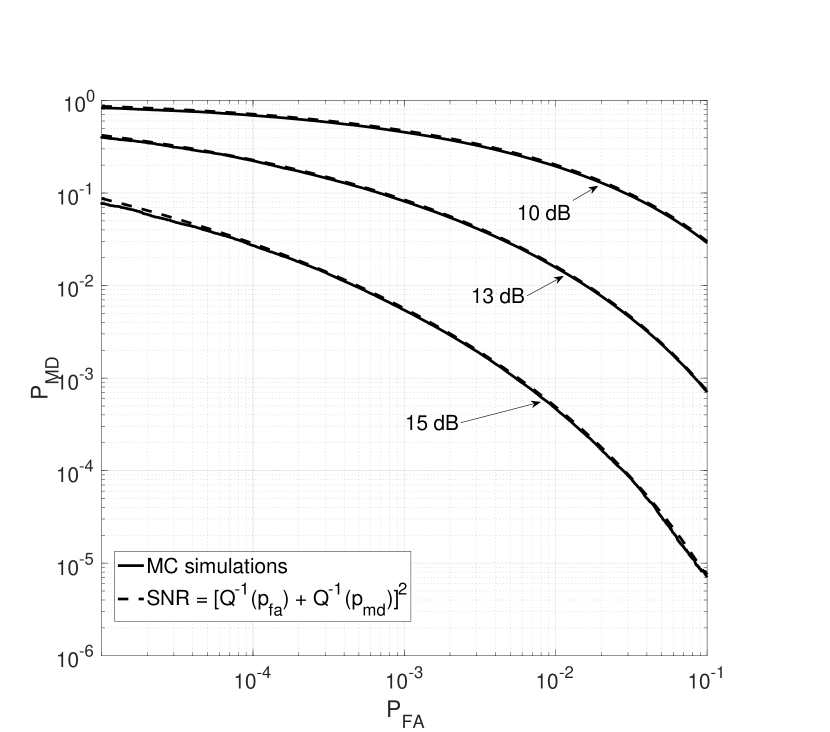
Figure 2: Detection error trade-off for $K_{a}=300$ and $J=12$. The solid curves are created by Monte-Carlo simulations of the channel (14) with subsequent likelihood-ratio test, where the threshold $\theta$ is varied. The dashed lines are calculated by (54).

VI Outer Channel

Let us assume that the inner decoder (SBS-MAP or AMP) has recovered the support of ${\bf s}=\sum_{k=1}^{K_{a}}{\bf m}_{k}$ such that the symbol-wise error probabilities are given by $p_{\text{md}}$ and $p_{\text{fa}}$. We have shown in the previous two sections how $p_{\text{md}}$ and $p_{\text{fa}}$ can be found in the asymptotic limit. The support of ${\bf s}$ is given by the OR-sum of the messages:

$$\hbox{\boldmath$\rho$}=\text{supp}({\bf s})=\bigvee_{k=1}^{K_{a}}{\bf m}_{k}$$ (56)

Let $\hat{\hbox{\boldmath$\rho$}}$ denote the estimated support vector. It can be interpreted as the output of $L$ uses of a vector OR-MAC with symbol-wise, asymmetric noise. We denote the lists of active indices in the $l$-th section by

$${\cal S}_{l}=\left\{i\in[1:2^{J}]:\hat{\rho}^{l}_{i}=1\right\}.$$ (57)

Given $L$ such lists, the outer decoder is tasked to recover the list of transmitted messages up to permutation. An outer code is a subset $\mathcal{C}\subset[1:2^{J}]^{L}$ of $|\mathcal{C}|=2^{JLR_{\text{out}}}$ codewords. An outer codeword can be equivalently represented as either a set of $L$ indices in $[1:2^{J}]$ or as a binary vector in $\mathbb{R}^{L2^{J}}$ with a single one in each section of size $2^{J}$.

Classical code constructions for the OR-MAC, like [46, 47], have been focussed on zero-error decoding, which does not allow for non-zero per-user-rates as $K_{a}\to\infty$, see e.g. [48] for a recent survey. Capacity bounds for the OR-MAC under the given input constraint have been derived in [49] and [50], where it was called the “T-user M-frequency noiseless MAC without intensity information” or “A-channel”. An asynchronous version of this channel was studied in [51]. Note, that the capacity bounds in the literature are combinatorial and hard to evaluate numerically for large numbers of $K_{a}$ and $2^{J}$. In the following we will show that, in the typical case of $K_{a}\ll 2^{J}$, a simple upper bound on the achievable rates based on the componentwise entropy is already tight.

From the channel coding theorem for discrete memoryless channels [4] it is known that a code with per-user-rate $R_{\text{out}}$ [bits/coded bits] and an arbitrarily small error probability exists if and only if

$$R_{\text{out}}<\frac{I({\bf m}_{1},...,{\bf m}_{K_{a}};\hat{\hbox{\boldmath$\rho$}})}{JK_{a}}.$$ (58)

The coding theorem assumes that each user has his own codebook, so the resulting rate constraint is an upper bound on the achievable rates of an outer code when every user has the same codebook. The mutual information is:

$$I({\bf m}_{1},...,{\bf m}_{K_{a}};\hat{{\bf s}})=H(\hat{{\bf s}})-H(\hat{{\bf s}}|{\bf m}_{1},...,{\bf m}_{K_{a}})$$ (59)

where

$$H(\hat{\hbox{\boldmath$\rho$}}|{\bf m}_{1},...,{\bf m}_{K_{a}})=2^{J}(p_{0}\mathcal{H}_{2}(p_{\text{fa}})+(1-p_{0})\mathcal{H}_{2}(p_{\text{md}}))$$ (60)

and $\mathcal{H}_{2}(\cdot)$ denotes the binary entropy function. The output entropy $H(\hat{{\bf s}})$ for general asymmetric noise is hard to compute. A simple upper bound on the entropy of the $2^{J}$-ary vector OR-channel can be obtained by the sum of the marginal entropies of $2^{J}$ independent binary-input binary-output channels. If we assume the coded messages to be uniformly distributed, i.e. $\mathbb{P}({\bf m}^{l}_{k}={\bf e}_{j})=2^{-J}$ for all $j=[1:2^{J}]$, then for all $i$

$$p(\rho_{i}=1)=1-p_{0}$$ (61)

with $p_{0}$ given in (8) and

$$p(\hat{\rho}_{i}=1)=(1-p_{0})(1-p_{\text{md}})+p_{0}p_{\text{fa}}$$ (62)

Therefore, after reordering, we get:

$$H(\hat{{\bf s}})\leq 2^{J}\mathcal{H}_{2}((1-p_{0})(1-p_{\text{fa}}-p_{\text{md}})+p_{\text{fa}})$$ (63)

Technically, this is only an upper bound, but we find numerically that it is very tight and furthermore, in the next section we will show that in the noiseless case it is actually achievable by an explicit outer code in the familiar limit $K_{a},J\to\infty$ with $J=\alpha\log_{2}K_{a}$. To find the limit of (63) we assume that $p_{\text{fa}}\leq cK_{a}/2^{J}=cK_{a}^{1-\alpha}$ for some constant $c>0$, i.e. the ratio of false positives to true positives remains at most constant as $K_{a},J\to\infty$. An equivalent condition is

$$\lim_{K_{a}\to\infty}\frac{\log_{2}p_{\text{fa}}}{\log_{2}K_{a}}\leq 1-\alpha$$ (64)

If this is not fulfilled the false positives dominate the entropy terms in the mutual information and the achievable rates go to zero. We use the fact that for small arguments, the binary entropy function becomes

$$\mathcal{H}_{2}(p)\approx p(1-\log_{2}p)$$ (65)

and that $(1-p_{0})\approx K_{a}/2^{J}$. With this, a straightforward calculation shows that

$$\lim_{K_{a},J\to\infty}\frac{I({\bf m}_{1},...,{\bf m}_{K_{a}};\hat{{\bf s}})}{JK_{a}}\leq(1-p_{\text{md}})\left(1-\frac{1}{\alpha}\right)$$ (66)

In the following we assume for simplicity that the inner decoder works error free, i.e. $p_{\text{fa}}=p_{\text{md}}=0$. Interestingly, the bound $1-\alpha^{-1}$ is achievable by a random code with a cover decoder, a construct often used in group testing literature. Given $\text{OR}(\mathcal{L})$, the OR-combination of $\mathcal{L}$, a list of $K_{a}$ codewords, the cover decoder goes through the whole codebook and produces a list of codewords that are covered by $\text{OR}(\mathcal{L})$. By construction the cover decoder will find all codewords in $\mathcal{L}$ and the error probability is governed by the number of false positives $n_{\text{fa}}$. We assume that if the decoder finds more than $K_{a}$ codewords, it discards exceeding codewords at random until the list contains only $K_{a}$ codewords. Therefore the per-user error probability of the cover decoder is given as $P_{e}=n_{\text{fa}}/(K_{a}+n_{\text{fa}})$. We write ${\bf c}_{1}\subset{\bf c}_{2}$ if a binary vector ${\bf c}_{1}$ is covered by a binary vector ${\bf c}_{2}$, that is if for all $i$ with $c_{1,i}=1$ also $c_{2,i}=1$.

Theorem 6.

Let $\mathcal{C}$ be an outer codebook of size $2^{LJR_{\text{out}}}$, where the position of each codeword in each section is chosen uniformly at random. Then the error probability of the cover decoder vanishes in the limit $L,K_{a},J\to\infty$ with $J=\alpha\log_{2}K_{a}$ for some $\alpha>1$ if

$$R_{\text{out}}<1-\frac{1}{\alpha}$$ (67)

$\hfill\square$

Proof.

Let $\mathcal{L}$ be a list of $K_{a}$ arbitrary codewords from $\mathcal{C}$. Then

$$P(n_{\text{fa}}\geq 1) =P\left(\bigcup_{{\bf c}\notin\mathcal{L}}\{{\bf c}\subset\text{OR}(\mathcal{L})\}\right)$$ (68)

$$\leq\sum_{{\bf c}\notin\mathcal{L}}P\left({\bf c}\subset\text{OR}\left(\mathcal{L}\right)\right)$$ (69)

$$\leq 2^{LJR_{\text{out}}}\max_{{\bf c}\notin\mathcal{L}}P\left({\bf c}\subset\text{OR}\left(\mathcal{L}\right)\right)$$ (70)

$$=2^{LJR_{\text{out}}}\max_{{\bf c}\notin\mathcal{L}}\prod_{l=1}^{L}P\left({\bf c}^{l}\subset\text{OR}\left(\mathcal{L}^{l}\right)\right)$$ (71)

$$=2^{LJR_{\text{out}}}\left(\frac{K_{a}}{2^{J}}\right)^{L}$$ (72)

$$=2^{LJR_{\text{out}}+L(1-\alpha)\log_{2}K_{a}}$$ (73)

$$=2^{LJ(R_{\text{out}}-(1-\alpha^{-1}))}$$ (74)

In the second line we have used the union bound. In the third line the non-negative sum is upper bounded by its maximum term times the number of codewords not in $\mathcal{L}$ which is $2^{LJR_{\text{out}}}-K_{a}\leq 2^{LJR_{\text{out}}}$. In the fourth line we have used that the entries of each section are chosen independently of each other. In the fifth line $\text{OR}(\mathcal{L}^{l})$ denotes the OR-combination of the $l$-th section of the codewords in $\mathcal{L}$. The probability that a random number from $[1:2^{J}]$ is contained in a fixed set of size $K_{a}$ is given by $1-(1-2^{-J})^{K_{a}}$, which becomes $K_{a}/2^{J}$ for small $K_{a}/2^{J}$. This probability is the same for all codewords not in $\mathcal{L}$ which allows to drop the maximum. It is apparent that the error probability vanishes for any $L$ and $J\to\infty$ if condition (67) is fulfilled. ∎

Remark 2.

The proof of Theorem 6 can easily be extended to include false positives. For that we introduce modified lists $\tilde{\text{OR}}(\mathcal{L}^{l})$, which in addition to the list of transmitted symbols in section $l$ also contain $n_{\text{fa}}$ random erroneous entries. If we assume that $n_{\text{fa}}=cK_{a}$ for some constant $c>0$ the result of Theorem 6 is unchanged. Since $p_{\text{fa}}=n_{\text{fa}}/2^{J}$, this condition is equivalent to (64).

We can also derive a finite length upper bound on the achievable outer rates with the cover decoder in a more direct, combinatorial way.

Theorem 7.

Any outer code that can guarantee error-free recovery under cover decoding for $K_{a}$ users with $L$-sections in the limit $K_{a},J\to\infty$ with $J=\alpha\log_{2}K_{a}$ has to satisfy:

$$R_{\text{out}}\leq 1-\frac{1}{\alpha}+\frac{1}{\alpha L}$$ (75)

$\hfill\square$

Proof.

We first show that any error free code has to satisfy

$$\frac{2^{LJR_{\text{out}}}}{K_{a}}\leq\frac{2^{JL}}{K_{a}^{L}}$$ (76)

To see this, assume an outer code that is error-free, i.e. for any list of $K_{a}$ codewords the OR-combination of theses codewords does not cover any other codeword that is not in the list. Then any two non-intersecting lists, $\mathcal{L}_{1}$ and $\mathcal{L}_{2}$, of $K_{a}$ codewords create two non-intersecting lists of $K_{a}^{L}$ possible sensewords. To see that they are non-intersecting, note, that due to the error-free property none of the codewords in $\mathcal{L}_{2}$ is covered by the OR-combination of all codewords from $\mathcal{L}_{1}$, which we denote by $\text{OR}(\mathcal{L}_{1})$. This means that each codeword from $\mathcal{L}_{2}$ differs from $\text{OR}(\mathcal{L}_{1})$ in at least one position. But this also means that any OR-combination of codewords from $\mathcal{L}_{2}$ differs from $\text{OR}(\mathcal{L}_{1})$ in at least one position.
Now divide the set of all $2^{LJR_{\text{out}}}$ codewords into distinct lists of length $K_{a}$, then each of these lists creates a distinct list of $K_{a}^{L}$ sensewords, whose total number has to be limited by the size of the space:

$$\frac{2^{LJR_{\text{out}}}}{K_{a}}K_{a}^{L}\leq 2^{JL}$$ (77)

This is precisely the statement of (76). If we use the scaling condition $2^{J}=K_{a}^{\alpha}$ and take the limit $K_{a},J\to\infty$ we get the statement of the theorem. ∎

For $L=1$ we get that $R_{\text{out}}\leq 1$, which can obviously be achieved, since for a single section no outer code is necessary.

VI-A Tree code

The first practical coding scheme for the outer OR-MAC with the sectionized structure has been presented in [17]. It works as follows: The $B$-bit message is divided into blocks of size $b_{1},b_{2},\ldots,b_{L}$ such that $\sum_{l}b_{l}=B$ and such that $b_{1}=J$ and $b_{l}<J$ for all $l=2,\ldots,L$. Each subblock $l=2,3,\ldots,L$ is augmented to size $J$ by appending $\pi_{l}=J-b_{l}$ parity bits, obtained using pseudo-random linear combinations of the information bits of the previous blocks $l^{\prime}<l$. Therefore, there is a one-to-one association between the set of all sequences of coded blocks and the paths of a tree of depth $L$. The pseudo-random parity-check equations generating the parity bits are identical for all users, i.e., each user makes use exactly of the same outer tree code. For more details on the outer coding scheme, please refer to [17].

Let ${\cal S}_{l},\ l=1,...,L$ be the list of active indices in the $l$-th section, defined in (57). Since the sections contain parity bits with parity profile $\{0,\pi_{2},\ldots,\pi_{L}\}$, not all message sequences in ${\cal S}_{1}\times{\cal S}_{2}\times\cdots\times{\cal S}_{L}$ are possible. The role of the outer decoder is to identify all possible message sequences, i.e., those corresponding to paths in the tree of the outer tree code [17]. The output list ${\cal L}$ is initialized as an empty list. Starting from $l=1$ and proceeding in order, the decoder converts the integer indices ${\cal S}_{l}$ back to their binary representation, separates data and parity bits, computes the parity checks for all the combinations with messages from the list ${\cal L}$ and extends only the paths in the tree which fulfill the parity checks. A precise analysis of the error probability in various asymptotic regimes is given in [17]. Specifically, the analysis shows that the error probability of the outer code goes to zero in the limit $K_{a},J\to\infty$ with $J=\alpha\log_{2}K_{a}$ and some $\alpha>1$ if the total number of parity bits $P=\sum_{l=2}^{L}\pi_{l}$ is chosen as ([17, Theorem 8 and 9])

1. $P=(L+\delta-1)\log_{2}K_{a}$ for some constant $\delta>0$ if all the parity bits are allocated in the last slots.

2. $P=c(L-1)\log_{2}K_{a}$ for some constant $c>1$ if the parity bits are allocated evenly at the end of each subslot except for the first.

In the first case the complexity scales like $\mathcal{O}(K_{a}^{R_{\text{out}}L}\log K_{a})$, since there is no pruning in the first $R_{\text{out}}L$ subslots, while in the second case the complexity scales linearly with $L$ like $\mathcal{O}(LK_{a}\log K_{a})$. The corresponding outer rates are

$$\begin{split}R_{\text{out}}&=B/(B+P)\\ &=1-P/(B+P)\\ &=1-P/(LJ)\\ &=1-\frac{L+\delta-1}{L\alpha}\\ &=1-\frac{1}{\alpha}+\frac{1}{L}\frac{\delta-1}{\alpha}\end{split}$$ (78)

for the case of all parity bits in the last sections and

$$\begin{split}R_{\text{out}}&=1-\frac{c(L-1)}{L\alpha}\\ &=1-\frac{c}{\alpha}-\frac{c}{L\alpha}\end{split}$$ (79)

for the case of equally distributed parity bits. In the limit $L\to\infty$ the achievable rates are therefore $R_{\text{out}}=1-1/\alpha$ and $R_{\text{out}}=1-c/\alpha$ respectively, which coincides with the asymptotic upper bound (66) for $p_{\text{md}}=0$ (up to a constant for the second case).

In Figure 3 and Figure 4 we compare empirical simulations with the developed theory. For the empirical results we fix $B=100$ bits and $L=8$. Furthermore, for various values of $J$ and $K_{a}$ we increase the number of parity bits until a per-user error probability $P_{e}<0.05$ is reached. In practice we use a mixture of the two types of parity profile described above. We choose the last section to be only parity bits, while the remaining parity bits are distributed uniformly over the sections $2,..,L-1$. The entropy bounds are calculated according to (63) with $p_{\text{fa}}=p_{\text{md}}=0$. In Figure 4 we plot the results as a function of $\alpha=J/\log_{2}K_{a}$. We can see that the achievable rates of the tree code with the used parity profile are very well described by the formula $R_{\text{out}}=1-\alpha^{-1}$ for different $J$ and $K_{a}$. Furthermore, we can see that the line $R_{\text{out}}=1-\alpha^{-1}$ is approached from above by the upper bound (63) as $J\to\infty$.

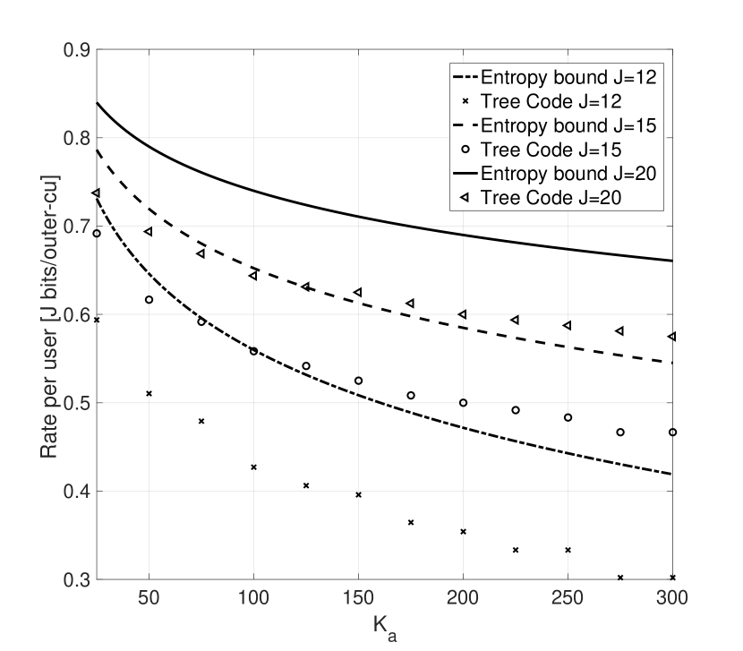
Figure 3: Achievable rates with the tree code with $L=8$ and $B=100$ bits together with the upper bound (63).

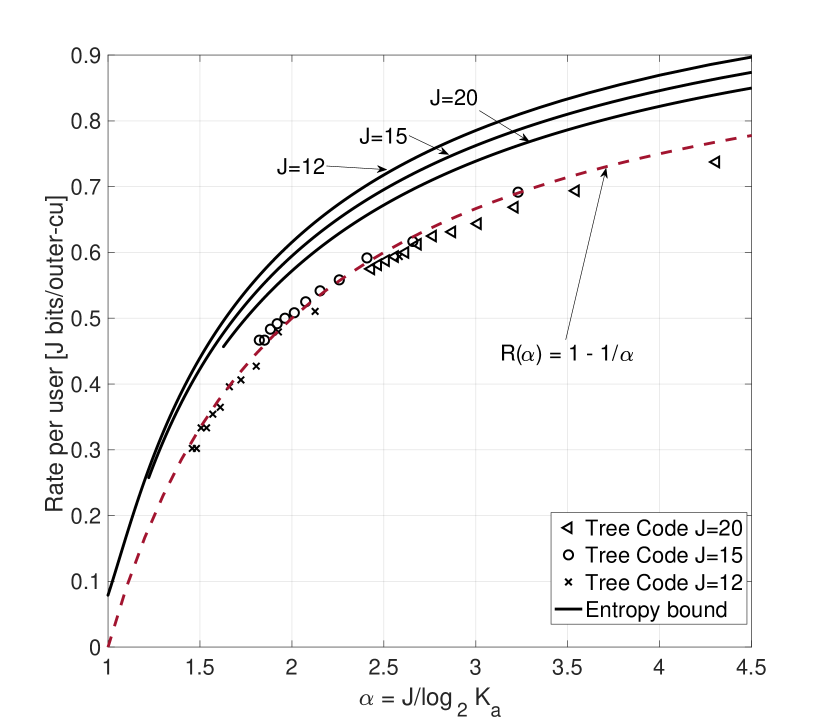
Figure 4: Achievable rates with the tree code with $L=8$ and $B=100$ bits together with the upper bound (63) as a function of $\alpha$.

VII Analysis of the concatenated scheme

Let us reformulate Theorem 5 in terms of the parameters of the concatenated code. Then the sum-rate is given as

$$S=K_{a}R=K_{a}R_{\text{in}}R_{\text{out}}=S_{\text{in}}R_{\text{out}}$$ (80)

and similarly we have

$$\frac{E_{b}}{N_{0}}=\frac{P}{RN_{0}}=\frac{\mathcal{E}_{\text{in}}}{R_{\text{out}}}.$$ (81)

As we have shown in the previous section, the best achievable outer rate is $R_{\text{out}}=1-\alpha^{-1}$, which turns out to coincide with the factor appearing in Theorem 5. Since the channel strength in the inner channel is given by $\eta\hat{P}$ and $\hat{P}=n{\sf SNR}/L=J{\sf SNR}/R_{\text{in}}=2J\mathcal{E}_{\text{in}}$, the channel strength goes to infinity with $J$ and the error probabilities $p_{\text{fa}}$ and $p_{\text{md}}$ in the outer channel vanish according to (54). An important condition to get the asymptotic limit $R_{\text{out}}=(1-p_{\text{md}})(1-\alpha^{-1})$ in (66) is (64), i.e. that the ratio of false positives to true positives remains at most constant. This condition requires that the channel strength in the inner channel has to grow fast enough to ensure that the probability of false alarms vanishes faster than the sparsity. In the following Theorem we show that the scaling condition for the error probability puts a constraint on the factor $\eta$.

Theorem 8.

Let $\eta\hat{P}$ be the channel strength in the scalar Gaussian channel (14). In the limit $K_{a},J\to\infty$ with $J=\alpha\log_{2}K_{a}$ for some $\alpha>1$ the condition (64) is fulfilled if and only if

$$\eta\geq\bar{\eta}$$ (82)

where $\bar{\eta}$ is given in (42). $\hfill\square$

Proof.

We show only the direction

$$\eta\geq\bar{\eta}\implies\lim_{K_{a}\to\infty}\frac{\log_{2}p_{\text{fa}}}{\log_{2}K_{a}}\leq 1-\alpha$$ (83)

the reverse implication can be shown similarly.
We can choose the points $p_{\text{md}}$ and $p_{\text{fa}}$ on the curve defined by (54) in a way that $Q^{-1}(p_{\text{md}})<\epsilon$ for some constant $\epsilon>0$. Therefore, for $\hat{P}=2J\mathcal{E}_{\text{in}}$

$$Q^{-1}(p_{\text{fa}})\geq\sqrt{\eta\hat{P}}-\epsilon=\sqrt{2\eta J\mathcal{E}_{\text{in}}}-\epsilon$$ (84)

so

$$p_{\text{fa}}\leq Q(\sqrt{2\eta J\mathcal{E}_{\text{in}}}-\epsilon)$$ (85)

and

$$\lim_{K_{a}\to\infty}\frac{\log_{2}p_{\text{fa}}}{\log_{2}K_{a}} \leq\lim_{K_{a}\to\infty}\frac{1}{\log_{2}(e)}\left(\frac{-\eta J\mathcal{E}_{\text{in}}}{\log_{2}K_{a}}+\frac{\mathcal{O}(\sqrt{J})}{\log_{2}K_{a}}\right)$$ (86)

$$=-\frac{\eta\alpha\mathcal{E}_{\text{in}}}{\log_{2}(e)}$$ (87)

where the first line follows from the standard bound on the Q-function $Q(x)\leq(2\pi)^{-1/2}\exp(-x^{2}/2)/x$. By reordering, we can see that $\eqref{eq:lim_log_p_fa}<1-\alpha$ if

$$\eta>\frac{1-\alpha^{-1}}{\log_{2}(e)\mathcal{E}_{\text{in}}}=\bar{\eta}$$ (88)

∎

The consequences of Theorem 8 for the concatenated code are summarized in the following Corollary.

Corollary 2.

Let $n,L,J,K_{a}\to\infty$ and $R,{\sf SNR}\to 0$ with fixed $E_{b}/N_{0}={\sf SNR}/(2R)$, $S=K_{a}R$ and $J=\alpha\log_{2}K_{a}$ for any $\alpha>1$. In this limit there is an outer code such that the concatenated code described in Section III with a random Gaussian codebook can be decoded with the AMP algorithm (9) and $P_{e}\to 0$ if and only if

$$S<\frac{1}{2}\left(\log_{2}e-(E_{b}/N_{0})^{-1}\right)$$ (89)

If the SBS-MAP estimator is used as inner decoder and the decoupling property holds true (Claim 1), reliable decoding is possible if and only if

$$S<\frac{1}{2}\log_{2}(1+K_{a}{\sf SNR})$$ (90)

$\square$

Proof.

The statement follows immediately from Theorems 5 and 8 together with the relation $\eta_{\text{loc}}^{*}<\bar{\eta}\leq 1$, which is discussed in the proof of Theorem 5. ∎

Remark 3.

In the case $K_{a}=1$ no outer code is necessary, so $R_{\text{in}}=R$ and furthermore $S_{\text{in}}=R$ and $2S_{\text{in}}\mathcal{E}_{\text{in}}={\sf SNR}$. Hence, if $K_{a}=1$ is fixed and $J\to\infty$, which corresponds to $\alpha\to\infty$, then Corollary 2 recovers the statements of [22, 23, 25], i.e. that SPARCs are reliable at rates up to the Shannon capacity $0.5\log_{2}(1+{\sf SNR})$ under optimal decoding. Also the algorithmic threshold (89) coincides with the result of [25]. In that sense Theorem 5 and Corollary 2 are an extension of [25] and show that SPARCs can achieve the optimal rate limit in the unsourced random access scenario. However, notice that the concept of our proof technique is simpler, since we make use of Theorem 3, which states that not only the sections are described by a decoupled channel model, but in the limit $J\to\infty$ also the individual components. So the result of Theorem 5 can be derived from the stationary points of a simple scalar-to-scalar function.

Remark 4.

In general, most classical multiple-access variants on the AWGN, where all the users are assumed to have their own codebook, can be represented as sparse recovery problems like (4). For that, let $K_{a}=1$ and identify the number of section with the number of users. The matrices ${\bf A}_{1},...,{\bf A}_{L}$ are then the codebooks of the individual users and $P_{l}$ are the transmit power coefficients of different users:

• Fixed $L$ in the limit $J,n\to\infty$ describes the classical AWGN Adder-MAC from [4], where each user has his own codebook.

• $L,J,n\to\infty$, where only a fraction of the sections are non-zero describes the many-access channel treated in [13]

• $J$ fixed and $L,n\to\infty$ describes specific version of the many-access MAC treated in [52, 14]

It is interesting, that in the first case Theorem 5 gives the correct result, after letting $\alpha\to\infty$, $K_{a}=1$ and $L=K$. The case of $J,n\to\infty$ at finite $L$ is not directly covered though by our analysis framework. Nonetheless, our empirical results (e.g. Figure 6) show a good agreement with the SE predictions even for small $L$. Especially the case $L=1$ is interesting since it resembles the U-RA formulation with random coding, as it was already noted in [52].

In Figure 5 and Figure 6 we visualize the results of Theorem 5. For that we fix $\alpha=2$. For various values of $J$ we set $K_{a}$ such that $J=\alpha\log_{2}K_{a}$. For each value of $R_{\text{in}}$ we then calculate $\eta_{\text{opt}}$ and $\eta_{\text{alg}}$ using the approximations of Theorem 2 and Corollary 1. We repeat this process with increasing ${\sf SNR}$ until $\eta_{\text{opt}}\hat{P}$ and $\eta_{\text{alg}}\hat{P}$ resp. reach a value of $(Q^{-1}(p_{\text{md}})+Q^{-1}(p_{\text{fa}}))^{2}$ where the error probabilities are chosen as $p_{\text{md}}=0.05/L$, with $L=8$, and $p_{\text{md}}=0.01K_{a}/2^{J}$. These are the solid lines in Figure 5 and Figure 6. The dashed lines are the threshold lines from Theorem 5. Additionally, in Figure 6 we plot empirical results, obtained by Monte-Carlo simulations with $L=8$, where the inner channel with the AMP decoder is simulated with increasing ${\sf SNR}$ until the error probabilities satisfy $p_{\text{md}}<0.05/L$ and $p_{\text{md}}<0.01K_{a}/2^{J}$, matching the values above. We can observe several interesting effects. We can see that the asymptotic trade-off curve $S_{\text{in}}(1-\alpha^{-1})=0.5\log_{2}(1+2S_{\text{in}}\mathcal{E}_{\text{in}})$ is approached from below by the curves for finite $J$. Also the finite length curves exhibit a region for small $S_{\text{in}}$, where $\mathcal{E}_{\text{in}}$ stays almost constant up to some value of $S_{\text{in}}$, and then it starts to grow linearly. Such a behavior was also observed in e.g. [52] in the context of finite-blocklength multiple access on the AWGN channel. This constant regions becomes smaller with increasing $J$ and disappears completely in the asymptotic limit. We can also see that there is a region of $S_{\text{in}}$ in that the algorithmic curve stays almost constant and matches the optimal curve. That is the region where there is only one unique minimum in the RS-potential. The empirical simulations in Figure 5 confirm the qualitative behavior of the calculated curves. The required energy stays constant over a large region of $S_{\text{in}}$ until some point, where it start to grow rapidly. Note, that Theorem 1 assumes infinite $L$, but nevertheless the theoretical results match the empirical simulations with $L=8$ very precisely. According to Theorem 5 in the limit $J\to\infty$ the required energy grows to infinity as $S_{\text{in}}$ approaches $\log_{2}(e)/[2(1-1/\alpha)]$. We can observe that this value is increased for finite $J$. In general, we can observe that the asymptotic algorithmic limit is very slowly approached from above. That has the interesting consequence, that for each $S_{\text{in}}$ there is a value $J^{*}$ below which the required energy decreases with $J$ and above which the required energy starts to increase again (see Figure 7 where this is visualized for $S_{\text{in}}=2$ with the same parameters as above). This reveals a limitation of the AMP algorithm, when used for sparse recovery, that only manifests when the size of the sections grows large while the inner rate is held constant. This goes against the intuition that the AMP performance should get better with increasing sections sizes because random fluctuations are averaged out. The sub-optimality of AMP and other iterative algorithms like belief-propagation has been noted several times, e.g. [36, 23, 26, 41]. The given analysis quantifies the sub-optimality from a different point of view, i.e. in the information theoretically interesting regime of constant inner rate.

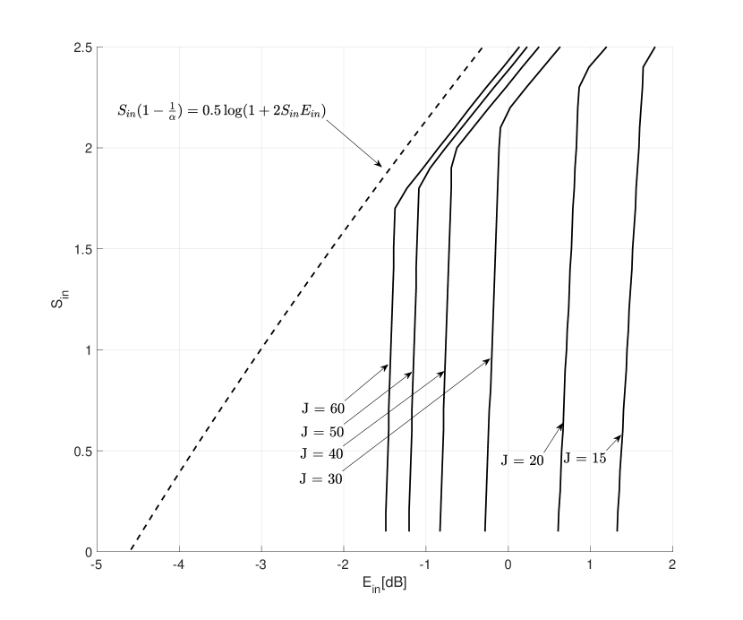
Figure 5: Required $\mathcal{E}_{\text{in}}$ to reach specific target error probabilities under optimal decoding and $J=\alpha\log_{2}K_{a}$ for $\alpha=2$ according to Claim 1 and Theorem 2. The dashed line is the asymptotic limit according to Theorem 5.

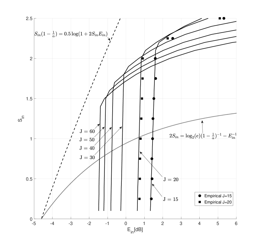
Figure 6: Required $\mathcal{E}_{\text{in}}$ to reach specific target error probabilities with AMP decoding and $J=\alpha\log_{2}K_{a}$ for $\alpha=2$ according to Theorem 1. The empirical simulations were conducted with $L=8$. The dashed lines are the asymptotic limits according to Theorem 5.

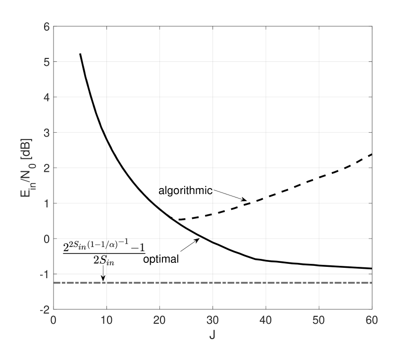
Figure 7: Required $\mathcal{E}_{\text{in}}$ to reach specific target error probabilities with $\alpha=2$ and $S_{\text{in}}=2$ according to Theorems 1,5 and Claim 1. The results show that the AMP estimate becomes increasingly suboptimal once $J$ passes a certain threshold around $J^{*}\approx 22$.

VIII Optimizing the Power Allocation

The foregoing asymptotic analysis has important implications for the code design. We have empirically observed that there is a critical number of users at which the required energy-per-bit increases sharply and that this critical number gets smaller as $J$ grows larger. According to the analytic insight developed in the previous section this behavior is to be attributed to the sub-optimality of the decoder, see Figure 6, and we expect the required energy to decrease further with $J$ if an optimal decoder is used. For single user sparse regression codes it is possible to get rid of the local minimum in the potential function. This has been achieved through a non-uniform power allocation in [23] and through spatial coupling in [24, 25, 26, 27]. More generally, it was shown in [53, 54] that in a set of identical copies of a recursive equation, which are described by some potential function, when the copies of the recursion are coupled in a special way, the potential of the coupled system has only one minimum, which coincides with the global minimum of the scalar potential function, even if the uncoupled potential has a local, non-global minimum. This phenomenon was termed threshold saturation in the context of belief-propagation decoding [55].

We focus on the power allocation approach, because it is easy to obtain an optimized power allocation for an AMP algorithm with separable denoising functions and a given input distribution. We present a linear programming algorithm to optimize the power allocation for the AMP algorithm that follows very closely the optimization procedure of [56], which was developed in the context of CDMA.

The denoising function in (10) was specific to a uniform power allocation $P_{l}=P/L$ for all $l$. For a generic power allocation we replace the componentwise denoising functions $f_{t,i}$ with ones that depend on the section index:

$$f_{t,i}^{l}(x)=\frac{\sqrt{\hat{P}_{l}}}{Z(x)}\sum_{k=0}^{K_{a}}p_{k}k\exp\left(\frac{1}{2\tau_{t}^{2}}\left(x-k\sqrt{\hat{P_{l}}}\right)^{2}\right)$$ (91)

where $\hat{P}_{l}=nP_{l}/L$ and

$$Z(x)=\sum_{k=0}^{K_{a}}p_{k}\exp\left(\frac{1}{2\tau_{t}^{2}}\left(x-k\sqrt{\hat{P_{l}}}\right)^{2}\right)$$ (92)

To analyse the error probability of this modified AMP algorithm in the asymptotic limit $L\to\infty$, we assume that the powers $P_{l}$ take values only in a finite set $\{\Pi_{1},...,\Pi_{I}\}$ and that the ratio of sections which use $\Pi_{i}$ is given by $\alpha_{i}=|\{l:P_{l}=\Pi_{i}\}|/L$ satisfying $\sum_{i=1}^{I}\alpha_{i}=1$ and $\sum_{i=1}^{I}\alpha_{i}\Pi_{i}=P$. We assume that these ratios stay constant as $L\to\infty$. According to the generalized SE in [32] the recursive equation which describes the behavior of the modified AMP algorithm is given by

$$\tau^{2}_{t+1}=\sigma_{w}^{2}+\lim_{L\to\infty}\frac{\beta}{L2^{J}}\mathbb{E}\left[\|\eta_{t}(\hbox{\boldmath$\theta$}+\tau_{t}{\bf Z})-\hbox{\boldmath$\theta$}\|_{2}^{2}\right]$$ (93)

where $\sigma^{2}_{w}=P^{-1}$,

$$\hbox{\boldmath$\theta$}=(\hbox{\boldmath$\theta$}^{1}|...|\hbox{\boldmath$\theta$}^{L})=\left(\left.\sqrt{\hat{P}_{1}}{\bf s}^{1}\right|...\left|\sqrt{\hat{P}_{L}}{\bf s}^{L}\right.\right)^{\top}$$ (94)

is a rescaled version of ${\bf s}$ and $\eta_{t}$ is componentwise given by $\eta_{t,i}^{l}=\sqrt{\hat{P}_{l}}f_{t,i}^{l}$. Since we choose $f_{t}^{l}=(f_{t,1}^{l},...,f_{t,2^{J}}^{l})$ to be separable the expected value in (93) decouples as follows

$$\begin{split}&\mathbb{E}\left[\|\eta_{t}(\hbox{\boldmath$\theta$}+\tau_{t}Z)-\hbox{\boldmath$\theta$}\|_{2}^{2}\right]=\\ &\sum_{l=1}^{L}\sum_{j=1}^{2^{J}}\mathbb{E}\left[\left(\sqrt{P}_{l}f_{t,j}^{l}\left(\sqrt{P}_{l}s^{l}_{j}+\tau_{t}Z\right)-\sqrt{P}_{l}s^{l}_{j}\right)^{2}\right]\end{split}$$ (95)

As $L$ goes to infinity the sum over $l$ converges to its mean for each $j$

$$\begin{split}\lim_{L\to\infty}\frac{1}{L}&\sum_{l=1}^{L}\mathbb{E}\left[\left(\sqrt{P}_{l}f_{t,j}^{l}\left(\sqrt{P}_{l}s^{l}_{j}+\tau_{t}Z\right)-\sqrt{P}_{l}s^{l}_{j}\right)^{2}\right]\\ &=\sum_{i=1}^{I}\alpha_{i}\hat{\Pi}_{i}\mathbb{E}\left[\left(f_{t,i}^{l}\left(\sqrt{\Pi}_{i}s+\tau_{t}Z\right)-s\right)^{2}\right]\end{split}$$ (96)

where now $s$ is a random variable distributed according to the marginal empirical distribution of ${\bf s}$ and $\hat{\Pi}_{i}=n\Pi_{i}/L=J\Pi_{i}/R_{\text{in}}$. This holds for each component $j$ and each $j$ has the same marginal distribution, so the sum over $j$ becomes redundant.

Remark 5.

We can see that in this calculation the sums over $j$ and $l$ are interchangeable. If $2^{J}$ is large enough the sum over $j$ already converges to its mean value and the sum over $l$ becomes redundant. This explains heuristically why we can observe a good correspondence between the state evolution and the empirical performance even for small $L$. Technically the exponential scaling regime with $\beta\to\infty$ is not covered by the result of [32].

Note, that the denoising functions $f_{t,i}^{l}$ were chosen precisely as the PME of $s$ in a scalar Gaussian channel like (14) with power $\sqrt{\hat{P}_{l}}$. So they minimize the MSE in (96) and by substituting $\tau^{2}=\eta^{-1}$ we get the fixed point condition

$$\eta^{-1}=1+\beta\sum_{i=1}^{I}\alpha_{i}\hat{\Pi}_{i}\text{mmse}(\eta\hat{\Pi}_{i}).$$ (97)

The function $\text{mmse}(t)$ is precisely the same as in (19). We can see that the right hand side of (97) is a linear combination of rescaled versions of the original MMSE function in (19). We can formulate the condition that (97) has no local minima besides the global minimum around $\eta=1$ as follows:

$$\begin{split}\underset{\hbox{\boldmath$\alpha$}}{\text{minimize}}\quad&\sum_{i=1}^{I}\alpha_{i}\Pi_{i}\\ \text{subject to}\quad&1+\beta\sum_{i=1}^{I}\alpha_{i}\hat{\Pi}_{i}\text{mmse}(\eta\hat{\Pi}_{i})<\eta^{-1}-\epsilon\\ &\forall\eta\in[0,1-\delta],\\ &\sum_{i=1}^{I}\alpha_{i}=1,\\ &\alpha_{i}\geq 0\end{split}$$ (98)

where $\epsilon,\delta>0$ are appropriately chosen slack variables. The optimization problem (98) is a linear program and therefore easily solvable. The discrete set of $\Pi_{i}$ is chosen as follows. For fixed $K_{a},J,R_{\text{in}}$ we set a target inner channel strength. We use Theorem 2 to determine the smallest power $P_{\text{opt}}$ such that for $\eta_{\text{opt}}$, the global minimizer of (16), it holds that $\eta_{\text{opt}}\hat{P}_{\text{opt}}$ exceeds the target inner channel strength. This $P_{\text{opt}}$ serves as lower bound on the set of $\Pi_{i}$. The upper bound is chosen arbitrary, e.g. $5P_{\text{opt}}$. The $\Pi_{i}$ are then chosen as a uniform discretisation of the interval $[P_{\text{opt}},5P_{\text{opt}}]$. In Figure 8 we visualize this for $K_{a}=300,J=20,R_{\text{in}}=0.0061$, where we have chosen the slack parameters $\epsilon=0.01,\delta=0.1$. The solution of (98) gives an optimal power distribution that puts weight only two values, $\Pi_{1}=P_{\text{opt}}$ and another value $P_{*}$ in a ratio of $\alpha_{1}\sim 0.81$ to $\alpha_{2}\sim 0.19$. The total average power $\alpha_{1}P_{\text{opt}}+\alpha_{2}P_{*}$ is about $0.5$dB smaller than $P_{\text{alg}}$, the power at which (16) has no local minimizers. This means by letting one fifth of the sections use a higher power it is possible to let the other four fifths of the section use the optimal power without having a local convergence point. In Figure 8 a) we plot

$$g(\eta)=1+\beta\left(\alpha_{1}\hat{P}_{\text{opt}}\text{mmse}(\eta\hat{P}_{\text{opt}})+\alpha_{2}\hat{P}_{*}\text{mmse}(\eta\hat{P}_{*})\right)-\eta^{-1}$$ (99)

and its counterparts without power allocation. Figure 8 b) shows the integral of $g(\eta)$, which resemble the RS-potential (16) with a non-uniform power allocation.

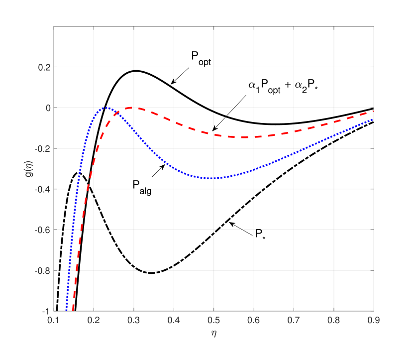
(a)

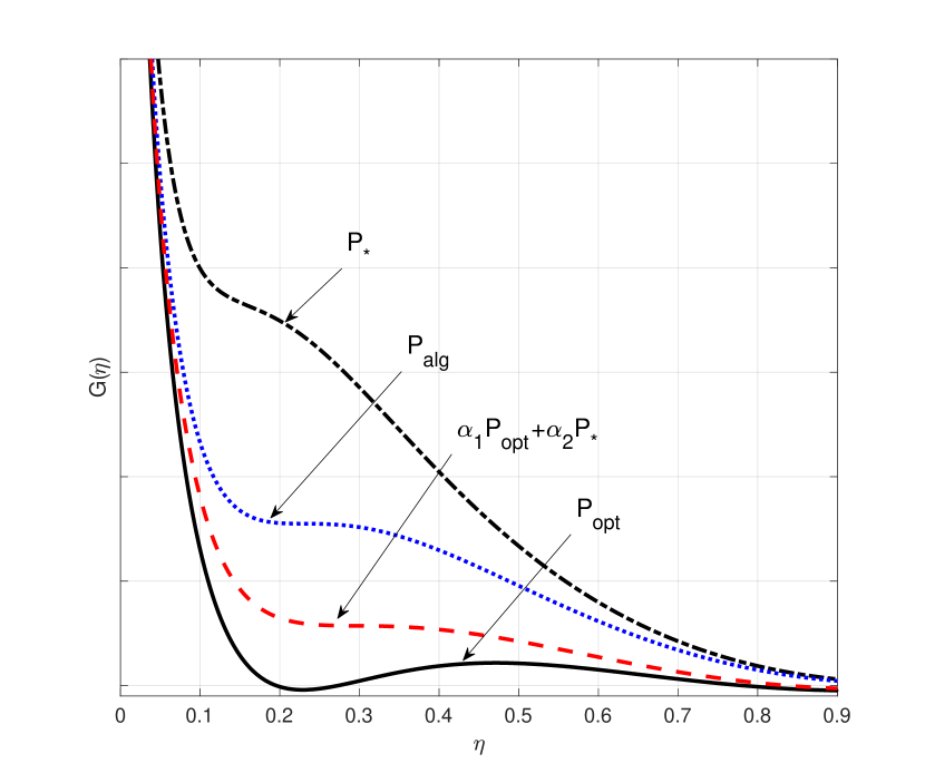
(b)

Figure 8: Visualization of the solution of the optimization problem for $K_{a}=300,R_{\text{in}}=0.0061,J=20$. The solution puts weights only on two powers $P_{\text{opt}}$ and $P_{*}\sim 1.9P_{\text{opt}}$ with ratios $\alpha_{1}=0.81$ and $\alpha_{2}=0.19$. The total power in the power allocated system is $\mathcal{E}_{\text{in}}=1.6$dB while the algorithmic threshold is $\mathcal{E}_{\text{in,alg}}=2.1$dB. So the power allocation in this case gives a gain of $0.5$dB.

The efficiency of the power allocation is demonstrated in Figure 9 with finite-length simulations. We choose $L=8,J=20$ and use the outer tree code with 0 parity bits in the first section, $20$ parity bits in the last, and alternating between 8 and 9 parity bits in the remaining sections. This leaves a total of $89$ data bits. We choose those numbers to stay below the typical number of 100 bits that is commonly used in IoT scenarios. The blocklength is chosen as $n=26229$, which results in $R_{\text{in}}=0.0061$ and a per-user spectral efficiency of $R_{\text{in}}R_{\text{out}}=0.0034$. To distribute the power as closely as possible to the optimized power allocation obtained above we choose two sections to have a power roughly twice as high as the remaining six sections. We can see that by using a power allocation a gain of about 0.5-1 dB is achievable, which matches the theoretical prediction. With the same parameters as above but $K_{a}=200$ we find that $P_{\text{alg}}=P_{\text{opt}}$. So the desired inner channel strength of $15$dB can be obtained by the AMP algorithm with a flat power allocation. In that case a non-uniform power allocation may be detrimental, because it could introduce unwanted local minima into (16). Indeed, simulations confirm that the 2-level power allocation that was effective for $K_{a}=300$ actually worsens the performance for $K_{a}\leq 250$. This means that the power allocation has to be tailored carefully to the expected parameters and it only improves the performance if there is a gap between $P_{\text{alg}}$ and $P_{\text{opt}}$.

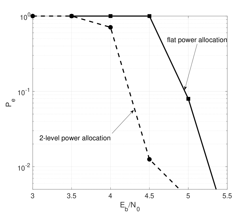
Figure 9: $J=20,L=8,B=89$ bits, $n=26229,R_{\text{out}}=0.55$, which leads to $R_{\text{in}}=0.0061$ and $\mu=0.0034$. $P_{e}$ is the per-user-probability of error.

IX Considerations for Practical Implementation

The denoising function in the AMP algorithm, (10) or its counterpart for non-uniform powers in (91), can be simplified if $K_{a}\ll 2^{J}$. Then the probabilities $p_{k}$ are very small for $k\geq 2$ and by neglecting them we get the modified denoising function

$$f_{t,i}^{\text{OR}}(x)=\sqrt{\hat{P}}\left(1+\frac{p_{0}}{1-p_{0}}\exp\left(\frac{\hat{P}-2\sqrt{\hat{P}x}}{2\tau_{t}^{2}}\right)\right)^{-1}$$ (100)

which we denote with the suffix OR because it is the PME in the channel (34). In the parameter range of our simulations we can see almost no difference between the full version (10) and the truncated OR-estimator (100). For moderate values of $2^{J}$ compared to $K_{a}$, we can improve on (100) slightly by taking into account $p_{2}$:

$$\begin{split}f_{t,i}^{\text{OR+}}(x)&=\frac{\sqrt{\hat{P}}}{Z(x)}\left(p_{1}\exp\left(-\frac{\left(x-\sqrt{\hat{P}}\right)^{2}}{2\tau_{t}^{2}}\right)\right.\\ &\left.+2(1-p_{0}-p_{1})\exp\left(-\frac{\left(x-2\sqrt{\hat{P}}\right)^{2}}{2\tau_{t}^{2}}\right)\right)\end{split}$$ (101)

where

$$\begin{split}Z(x)=&p_{0}\exp\left(-\frac{x^{2}}{2\tau_{t}^{2}}\right)+p_{1}\exp\left(-\frac{\left(x-\sqrt{\hat{P}}\right)^{2}}{2\tau_{t}^{2}}\right)\\ &+(1-p_{0}-p_{1})\exp\left(-\frac{\left(x-2\sqrt{\hat{P}}\right)^{2}}{2\tau_{t}^{2}}\right)\end{split}$$ (102)

If necessary, further terms can be included in the same way.

X Finite-length Simulations

In Figure 10 the required $E_{b}/N_{0}$ to achieve a per-user probability $P_{e}<0.05$ is shown. For the empirical curves with $J=15$ we use $B=100$ bits and $n=30000$ real symbols. For $J=20$ we use $B=89$ bits and $n=26226$ real symbols. This results in a per-user spectral efficiency of $\mu=0.0033$ and $\mu=0.0034$, which is the typical value used in comparable works [14, 19, 16, 17, 18]. As an inner decoder we use the AMP algorithm (9) with (101) as denoiser. After the inner decoder converged, in each section, the $K_{a}+\Delta$ largest entries are declared as active and added to the list $\mathcal{S}_{l}$ for the outer tree code. We use $\Delta=50$. For $J=15$ we use $L=16$ and the parity bits for the outer code are chosen as: $\hbox{\boldmath$\pi$}=(0,7,8,8,9,...,9,13,14)$. For $J=20$ we use $L=8$ and a parity bit distribution $\hbox{\boldmath$\pi$}=(0,9,8,9,8,9,8,20)$. The outer rates are $R_{\text{out}}=0.4167$ and $R_{\text{out}}=0.5563$ respectively. For the SE curves we first estimate the required effective inner channel strength by setting the error rates in the outer channel to $p_{\text{md}}=P_{e}/L$ and $p_{\text{fa}}=\Delta/2^{J}$. The required inner channel strength is then calculated by (54). We use the potential (16) to estimate the power to achieve the required inner channel strength. For the curves with power allocation we use the method of Section VIII to find the optimal power allocation for $K_{a}=300$. We can see that in both cases, $J=15$ and $J=20$, the required power decreases for $K_{a}=300$ but increases for all other values of $K_{a}$. So the power allocation has to be adapted to the expected number of users. The empirical values match the theoretically estimated SE curves very well, which confirms the precision of the asymptotic analysis, even though the number of sections is very small.

The obtained value of $4.3$ dB for $K_{a}=300$ is at the point of writing $0.7$ dB better than the best reported value of $5$ dB, which was achieved in [57]. For smaller values of $K_{a}$ other coding schemes have achieved better results, the best of which at the point of writing are [19] and [18], but both of those schemes have shown a rapid increase in required energy as $K_{a}$ grows large. In [57] an enhanced version of the discussed concatenated coding scheme was presented, where another outer code was used that enabled the passing of soft decoding information between the AMP decoder and the outer decoder, resulting in an turbo-like iterative decoding scheme, alternating between inner and outer decoder. With this type of decoding the required power for $K_{a}\leq 250$ is reduced significantly, but for $K_{a}=300$ the required power is still around $5$dB.

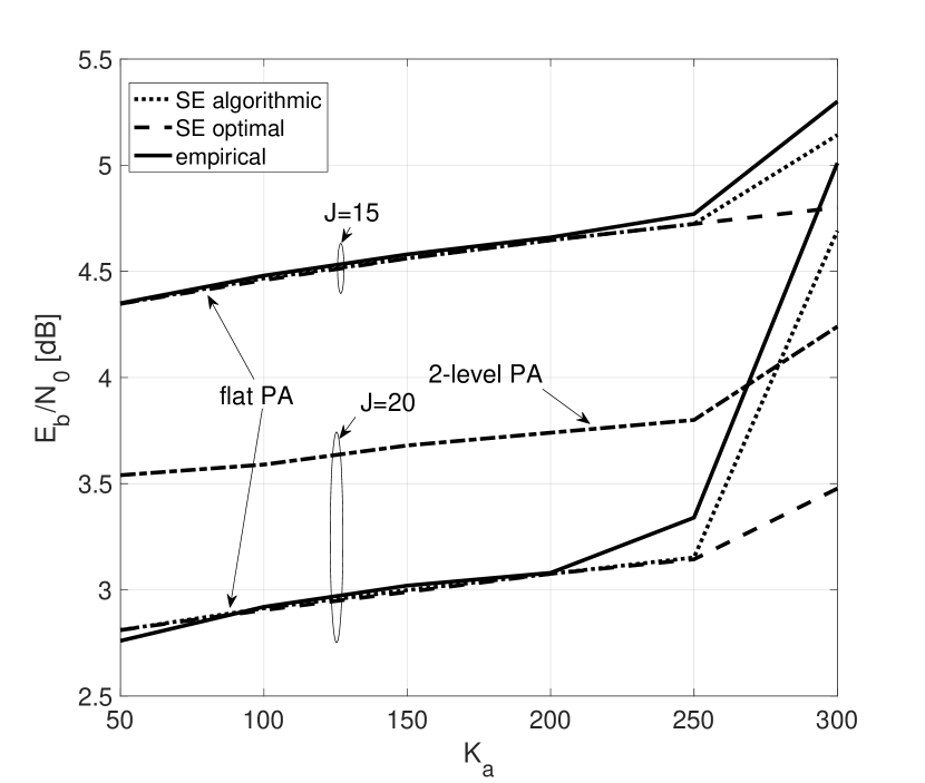
Figure 10: Required $E_{b}/N_{0}$ to achieve a per-user error probability $P_{e}<0.05$. For $J=15$ we used $B=100$, $n=30000$, and for $J=20$ we used $B=89$, $n=26229$.

XI Summary and Outlook

In this work we have introduced a concatenated coding construction that extends the concept of sparse regression codes to the unsourced random access scenario. In this construction an inner code is used as an efficient single user channel code for the AWGN channel and an outer code is used to resolve the multiple access interference. The structural similarity to the coupled compressed sensing scheme allowed us to use the tree code presented in [17] as an outer code. We use the AMP algorithm as inner decoder, for which we have introduced a low-complexity approximation to the Bayesian optimal denoiser. We introduced a decomposition of the channel into an inner and an outer channel to analyse the asymptotic limits under optimal decoding. Furthermore, we calculated the asymptotically required energy-per-bit of the inner AMP decoder and compared it to the optimal decoder. Finite-length simulations show that the calculated results describe the actual required energy-per-bit for a fixed per-user error probability very precisely. We find that as $J\to\infty$, where $2^{J}$ is the size of the outer alphabet, the achievable sum-rates of the concatenated code converge to the Shannon limit, even if the number of active users $K_{a}$ grows to infinity simultaneously, but much faster than $J$. This is in stark contrast to the typical information theoretic limit, where the size of the message is considered to be much larger than the number of active users. Therefore, it is noteworthy that even under short message length (compared to the number of users) and no coordination between users the Shannon limit can be achieved.

Unfortunately, also the difference in required energy between the AMP decoder and the optimal decoder grows rapidly with $J$ once $J$ surpasses a certain value that depends on the rate. When there is a difference in performance between the AMP and the optimal inner decoder, a non-uniform power allocation can be used to improve the performance of the AMP decoder. We present a linear programming algorithm to find an optimized power allocation. Although for small sum-spectral efficiencies existing U-RA coding schemes like [19, 18] are more energy-efficient than the presented scheme, we show that for a sum-spectral efficiency of 1 bit/c.u. and $K_{a}=300$ users the presented approach improves on existing ones by almost 1 dB. The good performance at high spectral efficiencies and the availability of a precise analysis make the presented coding scheme stand out among the existing U-RA approaches and therefore an interesting candidate for massive MTC.

The extension of the presented coding scheme and analysis to more general channel models incorporating fading, asynchronicity or multiple receivers seems to be in reach and promising research directions. Furthermore, the presented analysis can be seen as a basis to analyse the more complex turbo-like decoder of [57].

Appendix A Optimal product distribution

Lemma 1.

Let $\Omega\subset\mathbb{R}$ be some discrete set. Let $p({\bf s})$ with $p:\Omega^{2^{J}}\to\mathbb{R}_{+}$ be a probability mass function on $\Omega^{2^{J}}$. Let $p_{s_{1}}(s_{1}),....,p_{s_{2^{J}}}(s_{2^{J}})$ denote the marginals of $p({\bf s})$. Further let,

$$\mathcal{P}_{\text{prod}}:=\left\{q({\bf s})=\prod_{i=1}^{2^{J}}q_{i}(s_{i}),q_{i}:\Omega\to\mathbb{R}_{+}\middle|\sum_{s\in\Omega}q_{i}(s)=1\right\}$$ (103)

denote the space of product distributions on $\Omega^{2^{J}}$. Then

$$\operatorname*{arg\,min}_{q\in\mathcal{P}_{\text{prod}}}D(p\ \|\ q)=\prod_{i=1}^{2^{J}}p_{s_{i}}(s_{i})$$ (104)

Proof.

For a product distribution $q\in\mathcal{P}_{\text{prod}}$, $D(p\ \|\ q)$ can be expressed as:

$$D(p\ \|\ q) =\sum_{\bf s}p({\bf s})\log\frac{p({\bf s})}{q({\bf s})}$$ (105)

$$=\sum_{\bf s}p({\bf s})\log\frac{p({\bf s})}{\prod_{i}p_{s_{i}}(s_{i})}\frac{\prod_{i}p_{s_{i}}(s_{i})}{q({\bf s})}$$ (106)

$$=D\left(p\ \middle\|\ \prod_{i}p_{s_{i}}\right)+\sum_{\bf s}\sum_{i=1}^{2^{J}}p({\bf s})\log\frac{p_{s_{i}}(s_{i})}{q_{i}(s_{i})}$$ (107)

The first term is independent of $q$ and the second term can be rewritten as

$$\sum_{\bf s}\sum_{i=1}^{2^{J}}p({\bf s})\log\frac{p_{s_{i}}(s_{i})}{q_{i}(s_{i})}$$ (108)

$$=\sum_{i=1}^{2^{J}}\sum_{s_{i}}\left(\sum_{{\bf s}\setminus s_{i}}p({\bf s})\right)\log\frac{p_{s_{i}}(s_{i})}{q_{i}(s_{i})}$$ (109)

$$=\sum_{i=1}^{2^{J}}\sum_{s_{i}}p_{s_{i}}(s_{i})\log\frac{p_{s_{i}}(s_{i})}{q_{i}(s_{i})}$$ (110)

$$=\sum_{i=1}^{2^{J}}D(p_{s_{i}}\ \|\ q_{i})$$ (111)

which is non-negative and minimized by $q_{i}\equiv p_{s_{i}}$. ∎

Appendix B $D_{\text{KL}}$(Mult $\|$ Bin)

A vector $(z_{1},...,z_{2^{J}})$ is called multinomial distributed with parameter $n$ and probabilities $p_{1},...,p_{2^{J}}$ if

$$p({\bf z}) =\mathbb{P}(Z_{1}=z_{1},..,Z_{2^{J}}=z_{2^{J}})$$ (112)

$$=\begin{cases}\frac{n!}{z_{1}!\cdots z_{2^{J}}!}p_{1}^{z_{1}}\cdots p_{2^{J}}^{z_{2^{J}}}&\quad\sum_{i=1}^{2^{J}}z_{i}=n\\ 0&\quad\text{else}\end{cases}.$$ (113)

It follows from the multinomial theorem, that the distribution is normalized $\sum_{\bf z}p({\bf z})=1$. An important property of the multinomial distribution is that the marginals follow a binomial distribution:

$$p(Z_{i}=z_{i})=\sum_{{\bf z}\backslash z_{i}}\mathbb{P}(z_{1},...,z_{2^{J}})=\binom{n}{z_{i}}p_{i}^{z_{i}}(1-p_{i})^{n-z_{i}}$$ (114)

with covariance given by $\text{cov}(Z_{i},Z_{j})=-np_{i}p_{j}$.

Let $n=K_{a}$ and $p_{i}=2^{-J}$ for all $i=1,...,K_{a}$ and let $q(Z)$ denote the binomial distribution with parameters $n=K_{a}$ and $p_{i}=2^{-J}$. Then the marginals of $p$ are all identical and equal to $q(Z)$ and it holds

$$D_{\text{KL}}\left(p\ \middle\|\ \prod_{i=1}^{2^{J}}q_{i}\right) =\sum_{\bf z}p({\bf z})\log_{2}\frac{p({\bf z})}{q_{i}(z_{i})}$$ (115)

$$=-H(p)+2^{J}H(q)$$ (116)

where $H(p)$ denotes the entropy of the multinomial distribution $p$ and $H(q)$ the entropy of the binomial distribution $q$. Both entropies are well known and given by

$$H(p)=JK_{a}-\log_{2}K_{a}!$$ (117)

$$+2^{J}\sum_{t=0}^{K_{a}}{{K_{a}}\choose{t}}\left(2^{-J}\right)^{t}\left(1-2^{-J}\right)^{K_{a}-t}\log_{2}t!$$ (118)

and

$$H(q) =-\log_{2}K_{a}!+\mathbb{E}_{q}[\log Z!]+\mathbb{E}_{q}[\log(K_{a}-Z)!]$$ (119)

$$+J\mathbb{E}_{q}[Z]-\mathbb{E}_{q}[K_{a}-Z]\log_{2}(1-2^{-J})$$ (120)

We have $\mathbb{E}_{q}[Z]=K_{a}/2^{J}$ and $\mathbb{E}_{q}[K_{a}-Z]=K_{a}-K_{a}/2^{J}$. In the limit for large $J$, we can expand $\mathbb{E}_{q}[\log_{2}(K_{a}-Z)!]$ in terms of $2^{-J}$ and get:

$$\mathbb{E}_{q}[\log_{2}(K_{a}-Z)!]=\log_{2}K_{a}!-\frac{K_{a}}{2^{J}}\log_{2}K_{a}+\mathcal{O}\left(\frac{1}{2^{2J}}\right).$$ (121)

Inserting this, (118) and (120) into (116), many terms cancel and we get:

$$D_{\text{KL}}\left(p\ \middle\|\ \prod_{i=1}^{K_{a}}q_{i}\right)$$ (122)

$$=\log_{2}K_{a}!-K_{a}(2^{J}-1)\log_{2}(1-2^{-J})-K_{a}\log_{2}K_{a}$$ (123)

Using $\log_{2}(1-2^{-J})=-\log_{2}(e)/2^{J}+\mathcal{O}(1/2^{2J})$ for large $J$ and the Stirling approximation $\log_{2}K_{a}!=K_{a}\log_{2}K_{a}-K_{a}\log_{2}e+\mathcal{O}(\log K_{a})$ we get

$$D_{\text{KL}}\left(p({\bf x})\ \middle\|\ \prod_{i=1}^{K_{a}}q_{i}(x_{i})\right)=\mathcal{O}(\log K_{a})-\frac{K_{a}\log_{2}e}{2^{J}}.$$ (124)

which implies (29).

Appendix C Exponential $L^{1}$ convergence implies exponential convergence in measure

Theorem 9.

Let $(f_{J})_{J=1,2,...}$ be a sequence of integrable functions s.t.

$$\|f_{J}-f\|_{L^{1}}\leq\frac{c}{2^{J}}$$ (125)

for some constant $c>0$ and all large enough $J$. For any $\delta>0$ there is a $J_{\delta}$ such that for all $J\geq J_{\delta}$

$$|f_{J}(t)-f(t)|\leq\frac{\sqrt{J}}{\delta 2^{J}}$$ (126)

holds for all $t$ except for a set of size $\mathcal{O}(\delta J^{-1/2})$. $\hfill\square$

Proof.

Let $\epsilon>0$ then

$$\sum_{j=J}^{\infty}\|f_{j}-f\|_{L^{1}}\leq\frac{c}{2^{J-1}}<\epsilon\frac{\sqrt{J}}{\delta 2^{J}}$$ (127)

holds for all

$$J>J_{\delta}=\left(\frac{2c\delta}{\epsilon}\right)^{2}$$ (128)

where we have used condition (125) and the formula

$$\sum_{j=J}^{\infty}2^{-j}=2^{-(J-1)}.$$ (129)

Now define the sets

$$A_{j}=\left\{t:|f_{j}(t)-f(t)|>\frac{\sqrt{j}}{\delta 2^{j}}\right\}$$ (130)

and let $\mu(A_{j})$ denote the Lebesgue measure of $A_{j}$. Then it follows from elementary properties of the integral that

$$\sum_{j=J}^{\infty}\mu(A_{j})\frac{\sqrt{J}}{\delta 2^{J}}<\sum_{j=J}^{\infty}\|f_{j}-f\|_{L^{1}}<\epsilon\frac{\sqrt{J}}{\delta 2^{J}}$$ (131)

and so

$$\mu\left(\bigcup_{j=J}^{\infty}A_{j}\right)\leq\sum_{j=J}^{\infty}\mu(A_{j})<\epsilon$$ (132)

Let $\mathcal{A}_{J}:=\bigcup_{j=J}^{\infty}A_{j}$, then

$$\mathcal{A}_{J}^{c}=\left\{t:|f_{j}(t)-f(t)|\leq\frac{\sqrt{J}}{\delta 2^{J}},\ \forall j\geq J\right\}$$ (133)

and so (132) states that $\mu(\mathcal{A}_{J})$, the measure of the set of points on which the pointwise convergence does not hold, can be made arbitrarily small. More precisely, it follows from (128) that

$$\mu(\mathcal{A}_{J})=\mathcal{O}\left(\frac{\delta}{\sqrt{J}}\right)$$ (134)

∎

Appendix D Proof of Theorem 3

Let

$$q(k)=p_{k}$$ (135)

for $k=0,..,K_{a}$, where $p_{k}$ are the binomial probabilities defined in (7) and

$$q_{\text{OR}}(0) =p_{0}$$ (136)

$$q_{\text{OR}}(1) =1-p_{0}.$$ (137)

Let $r,s,z$ be jointly distributed according to the Gaussian model

$$r=\sqrt{t}s+z,$$ (138)

with $z\sim\mathcal{N}(0,1)$ independent of $s$ for some fixed $t\geq 0$ and $s$ distributed according to $q$. Let $\text{mmse}(t)$ be the MMSE of estimating $s$ from the Gaussian observation $r$ and let $f(r)$ be the PME of $s$, given by

$$f(r)=\frac{1}{Z(r)}\sum_{k=0}^{K_{a}}p_{k}ke^{-\left(r-k\sqrt{t}\right)^{2}/2}$$ (139)

with

$$Z(r)=\sum_{k=0}^{K_{a}}p_{k}e^{-\left(r-k\sqrt{t}\right)^{2}/2}$$ (140)

Let $f^{\text{OR}}(r)$ be the mismatched PME, which estimates $s$ from $r$ assuming that $s$ is distributed according to $q_{\text{OR}}$. It is given by

$$f^{\text{OR}}(r)=\frac{(1-p_{0})e^{-\left(r-\sqrt{t}\right)^{2}/2}}{Z^{\text{OR}}(r)}$$ (141)

with

$$Z^{\text{OR}}(r)=p_{0}e^{-r^{2}/2}+(1-p_{0})e^{-\left(r-\sqrt{t}\right)^{2}/2}$$ (142)

Let $\text{mmse}_{\text{OR}}(t)$ be the mean square error of $f^{\text{OR}}(r)$. Since $f^{\text{OR}}(r)$ is mismatched we have $\text{mmse}(t)\leq\text{mmse}_{\text{OR}}(t)$ and it holds:

$$0 \leq\text{mmse}_{\text{OR}}(t)-\text{mmse}(t)$$ (143)

$$=\sum_{k=0}^{K_{a}}p_{k}\mathbb{E}\left\{\left[k-f^{\text{OR}}\left(\sqrt{t}k+z\right)\right]^{2}-[k-f(\sqrt{t}k+z)]^{2}\right\}$$ (144)

$$=p_{0}\mathbb{E}\left\{\left[f^{\text{OR}}(z)\right]^{2}-\left[f(z)\right]^{2}\right\}$$ (145)

$$+p_{1}\mathbb{E}\left\{\left[1-f^{\text{OR}}\left(\sqrt{t}+z\right)\right]^{2}-\left[1-f\left(\sqrt{t}+z\right)\right]^{2}\right\}$$ (146)

$$+\sum_{k=2}^{K_{a}}p_{k}\mathbb{E}\left\{\left[k-f^{\text{OR}}\left(\sqrt{t}k+z\right)\right]^{2}-\left[k-f\left(\sqrt{t}k+z\right)\right]^{2}\right\}$$ (147)

We can bound the terms (145) - (147) individually. Since $0\leq f^{\text{OR}}(r)\leq 1$, (147) is bound by

$$\eqref{eq:mse_3} \leq\sum_{k=2}^{K_{a}}p_{k}k^{2}$$ (148)

$$=\text{Var}(s)+[\mathbb{E}(s)]^{2}-p_{1}$$ (149)

$$=\frac{K_{a}}{2^{J}}\left(1-\frac{K_{a}}{2^{J}}\right)+\frac{K_{a}^{2}}{2^{2J}}-\frac{K_{a}}{2^{J}}\left(1-2^{-J}\right)^{K_{a}-1}$$ (150)

$$=\mathcal{O}\left(\frac{K_{a}^{2}}{2^{2J}}\right)$$ (151)

For the remaining terms we split the expected values over $z$ in (145) and $\eqref{eq:mse_2}$ in two parts, depending on whether $Z(r)=Z(\sqrt{t}+z)$ is smaller or larger than $Z^{\text{OR}}(r)$.

D-1 $Z(r)\leq Z^{\text{OR}}(r)$

We have:

$$f^{\text{OR}}(r) =\frac{1}{Z^{\text{OR}}(r)}(1-p_{0})e^{-\left(r-\sqrt{t}\right)^{2}/2}$$ (152)

$$\leq\frac{1}{Z(r)}(1-p_{0})e^{-\left(r-\sqrt{t}\right)^{2}/2}$$ (153)

and

$$f(r) =\frac{1}{Z(r)}\sum_{k=0}^{K_{a}}p_{k}ke^{-\left(r-\sqrt{t}k\right)^{2}/2}$$ (154)

$$\geq\frac{1}{Z(r)}p_{1}e^{-\left(r-\sqrt{t}\right)^{2}/2}$$ (155)

because all the summands are non-negative. It follows for all $r$:

$$[f^{\text{OR}}(r)]^{2}-[f(r)]^{2}$$ (156)

$$\leq\left[\frac{p_{1}e^{-\left(r-\sqrt{t}\right)^{2}/2}}{Z(r)}\right]^{2}\left[\left(\frac{1-p_{0}}{p_{1}}\right)^{2}-1\right]$$ (157)

$$\leq\left[\left(\frac{1-p_{0}}{p_{1}}\right)^{2}-1\right]$$ (158)

$$=\left[\left(\frac{1-(1-2^{-J})^{K_{a}}}{\frac{K_{a}}{2^{J}}(1-2^{-J})^{K_{a}-1}}\right)^{2}-1\right]$$ (159)

$$\leq\mathcal{O}\left(\frac{K_{a}^{2}}{2^{2J}}\right)$$ (160)

which bounds the integral in $\eqref{eq:mse_1}$ on the set $\{Z(z)\leq Z^{\text{OR}}(z)\}$. For (146) notice that

$$\left[1-f^{\text{OR}}(r)\right]^{2}-[1-f(r)]^{2}$$ (161)

$$=f^{\text{OR}}(r)^{2}-f(r)^{2}+2\left[f(r)-f^{\text{OR}}(r)\right]$$ (162)

The first term was already bound in (160), we bound the second term by

$$f(r)-f^{\text{OR}}(r)$$ (163)

$$=\left[1-f^{\text{OR}}(r)\right]-[1-f(r)]$$ (164)

$$=\frac{p_{0}e^{-r^{2}/2}}{Z^{\text{OR}}(r)}-\frac{p_{0}e^{-r^{2}/2}+\sum_{k=1}^{K_{a}}p_{k}(1-k)e^{-\left(r-\sqrt{t}k\right)^{2}/2}}{Z(r)}$$ (165)

$$\leq\frac{1}{Z(r)}\sum_{k=2}^{K_{a}}p_{k}(k-1)e^{-\left(r-\sqrt{t}k\right)^{2}/2}$$ (166)

$$\leq\frac{1}{Z(r)}\max_{k\geq 2}\left\{e^{-\left(r-\sqrt{t}k\right)^{2}/2}\right\}\sum_{k=2}^{K_{a}}kp_{k}$$ (167)

$$=\frac{1}{Z(r)}\max_{k\geq 2}\left\{e^{-\left(r-\sqrt{t}k\right)^{2}/2}\right\}\left(\frac{K_{a}}{2^{J}}-p_{1}\right)$$ (168)

$$=\frac{e^{-\left(r-\sqrt{t}k^{*}\right)^{2}/2}}{p_{1}e^{-\left(r-\sqrt{t}\right)^{2}/2}}\mathcal{O}\left(\frac{K_{a}^{2}}{2^{2J}}\right)$$ (169)

where $k^{*}=\operatorname*{arg\,max}_{k\geq 2}\left\{\exp(-(r-\sqrt{t}k)^{2}/2)\right\}$. For the last line, notice that $Z(r)\geq p_{k}\exp(-(r-\sqrt{t}k)^{2}/2)$ for all $k$ and especially for $k=1$. In (169) we have $r=\sqrt{t}+z$. For the expected value in (146) we have to integrate over $z$, restricted to the values of $z$ for which $Z(r)\leq Z^{\text{OR}}(r)$. Since

$$\int_{-\infty}^{\infty}e^{-z^{2}/2}\frac{e^{-(z-\sqrt{t}(k^{*}-1))^{2}/2}}{p_{1}e^{-z^{2}/2}}=\frac{1}{p_{1}}$$ (170)

and the integrand is non-negative, the same integral, restricted to $\{z:Z(\sqrt{t}+z)\leq Z^{\text{OR}}(\sqrt{t}+z)\}$, is also bounded by $1/p_{1}$.

D-2 $Z(r)>Z^{\text{OR}}(r)$

Let $r$ be such that, $Z(r)>Z^{\text{OR}}(r)$. It holds that

$$f^{\text{OR}}(r) =1-\frac{p_{0}e^{-r^{2}/2}}{Z^{\text{OR}}(r)}$$ (171)

$$\leq 1-\frac{p_{0}e^{-r^{2}/2}}{Z(r)}$$ (172)

$$=\frac{1}{Z(r)}\sum_{k=1}^{K_{a}}p_{k}e^{-\left(r-k\sqrt{t}\right)^{2}/2}$$ (173)

$$\leq\frac{1}{Z(r)}\sum_{k=1}^{K_{a}}kp_{k}e^{-\left(r-k\sqrt{t}\right)^{2}/2}$$ (174)

$$=f(r)$$ (175)

Since both terms are non-negative we get

$$f^{\text{OR}}(r)^{2}-f(r)^{2}\leq 0$$ (176)

which, together with (160), shows that (145) is bounded by a term of order $\mathcal{O}\left(\frac{K_{a}^{2}}{2^{2J}}\right)$.

For (146), the same argumentation as in (162) holds and it remains to bound $f(r)-f^{\text{OR}}(r)$. We have that

$$f(r)-f^{\text{OR}}(r)$$ (177)

$$=\frac{1}{Z(r)}\sum_{k=1}^{K_{a}}kp_{k}e^{-\left(r-k\sqrt{t}\right)^{2}/2}-\frac{1}{Z^{\text{OR}}(r)}(1-p_{0})e^{-\left(r-\sqrt{t}\right)^{2}/2}$$ (178)

$$\leq\frac{1}{Z(r)}\sum_{k=1}^{K_{a}}kp_{k}e^{-\left(r-k\sqrt{t}\right)^{2}/2}-\frac{1}{Z(r)}(1-p_{0})e^{-\left(r-\sqrt{t}\right)^{2}/2}$$ (179)

$$\leq\frac{1}{Z(r)}\sum_{k=2}^{K_{a}}kp_{k}e^{-\left(r-k\sqrt{t}\right)^{2}/2}$$ (180)

$$\leq\frac{1}{Z(r)}\max_{k\geq 2}\left\{e^{-\left(r-\sqrt{t}k\right)^{2}/2}\right\}\left(\frac{K_{a}}{2^{J}}-p_{1}\right)$$ (181)

$$=\frac{e^{-\left(r-\sqrt{t}k^{*}\right)^{2}/2}}{p_{1}e^{-\left(r-\sqrt{t}\right)^{2}/2}}\mathcal{O}\left(\frac{K_{a}^{2}}{2^{2J}}\right)$$ (182)

This is the same term as in (182), for which we have shown that its expected value over $z$ is bounded by $p_{1}^{-1}\mathcal{O}(K_{a}^{2}/2^{2J})$. (182), together with (169), shows that $f(r)-f^{\text{OR}}(r)$ is bounded by $p_{1}^{-1}\mathcal{O}(K_{a}^{2}/2^{2J})$ for all $r$. (169) and (176) show that $f^{\text{OR}}(r)^{2}-f(r)^{2}=\mathcal{O}(K_{a}^{2}/2^{2J})$ for all $r$, and therefore, by (162), also (146) is bound by a term of order $\mathcal{O}\left(\frac{K_{a}^{2}}{2^{2J}}\right)$. This concludes the proof of Theorem 3.

Appendix E Proof of Theorem 4

The RS-potential (37), rescaled by $\beta/2^{J}$ takes the form

$$i^{\text{RS}}(\eta)=\frac{R_{\text{in}}2^{J}}{J}I(\eta\hat{P})+\frac{\log_{2}e}{2}[(\eta-1)-\ln\eta]$$ (183)

with the mutual information

$$I(\eta\hat{P}):=I(X;Y)=H(Y)-H(Y|X)$$ (184)

for $P(X=0)=p_{0}$, $P(X=1)=1-p_{0}$ and $Y=(\eta\hat{P})^{\frac{1}{2}}X+Z$, for $Z\sim\mathcal{N}(0,1)$ independent of $X$. The mutual information $I(\eta\hat{P})$ can be evaluated as follows. First, note that in an additive channel $H(Y|X)=H(Z)$, so $H(Y|X)$ is independent of $\eta$ and therefore we can ignore it when evaluating $i^{\text{RS}}(\eta)$. The distribution of $Y$ is given by

$$\begin{split}p(y)&=p_{0}p(y|x=0)+(1-p_{0})p(y|x=1)\\ &=\frac{p_{0}}{\sqrt{2\pi}}\exp\left(-\frac{y^{2}}{2}\right)+\frac{1-p_{0}}{\sqrt{2\pi}}\exp\left(-\frac{1}{2}\left(y-(\eta\hat{P})^{\frac{1}{2}}\right)^{2}\right),\end{split}$$ (185)

so the differential output entropy $H(Y)=-\int p(y)\log_{2}p(y)\mathrm{d}y$ can be split into the sum of two parts. Define $H_{0}$ and $H_{1}$ respectively by

$$H_{0}:=-\frac{1}{\sqrt{2\pi}}\int_{-\infty}^{\infty}\exp\left(-\frac{y^{2}}{2}\right)\log_{2}(p(y))\mathrm{d}y$$ (186)

and

$$\begin{split}H_{1}&:=-\frac{1}{\sqrt{2\pi}}\int_{-\infty}^{\infty}\exp\left(-\frac{1}{2}\left(y-(\eta\hat{P})^{\frac{1}{2}}\right)^{2}\right)\log_{2}(p(y))\mathrm{d}y\\ &=-\frac{1}{\sqrt{2\pi}}\int_{-\infty}^{\infty}\exp\left(-\frac{y^{2}}{2}\right)\log_{2}\left(p\left(y+(\eta\hat{P})^{\frac{1}{2}}\right)\right)\mathrm{d}y\end{split}$$ (187)

such that the following relation holds:

$$I(\eta\hat{P})=p_{0}H_{0}+(1-p_{0})H_{1}.$$ (188)

Taking into account the scaling factor in (183) and using that $\lim_{J\to\infty}2^{J}(1-p_{0})=K_{a}$ and $\lim_{J\to\infty}p_{0}=1$ we get that

$$\begin{split}\lim_{J\to\infty}\frac{R_{\text{in}}2^{J}}{J}I(\eta\hat{P})&=\lim_{J\to\infty}\left(\frac{R_{\text{in}}2^{J}}{J}H_{0}+\frac{S}{J}H_{1}\right)\end{split}$$ (189)

Now let us take a closer look at $\log_{2}p(y)=\log_{2}(e)\ln p(y)$ which appears in both $H_{0}$ and $H_{1}$. Let $x_{1},x_{2}>0$ with $x_{2}>x_{1}$. Then for the logarithm of the sum of exponentials it holds that

$$-\ln(e^{-x_{1}}+e^{-x_{2}})=x_{1}+\ln(1+e^{-(x_{2}-x_{1})}).$$ (190)

The error term $\ln(1+e^{-(x_{2}-x_{1})})$ decays exponentially as the difference $x_{2}-x_{1}$ grows. Since $p(y)$ is the sum of two exponentials we can approximate $\ln p(y)$ by:

$$\begin{split}-\ln p(y)\approx\min\left\{\frac{y^{2}}{2}-\ln(p_{0}),\frac{1}{2}\left(y-(\eta\hat{P})^{\frac{1}{2}}\right)^{2}-\ln(1-p_{0})\right\}\end{split}$$ (191)

This approximation is justified, since the difference of the two exponents in $p(y)$ is proportional to $\sqrt{J}$, and so it grows large with $J$. First, note, that since $\min\{a,b\}\leq a$ and $\min\{a,b\}\leq b$ holds for all $a,b\in\mathbb{R}$, $-\ln p(y)\leq y^{2}/2-\ln(1-p_{0})$ as well as $-\ln p(y+(\eta\hat{P})^{\frac{1}{2}})\leq y^{2}/2+\ln(2^{J}/K_{a})$. This means that each of the integrands in $H_{0}$ and $H_{1}/J$ resp. is bounded uniformly, for all $J$, by an integrable function. This allows us to evaluate the integrals by using Lebesgue’s theorem on dominated convergence. For this purpose we need to calculate the pointwise limits of $\ln p(y)$ and $\ln p(y+(\eta\hat{P})^{\frac{1}{2}})/J$. The theorem on dominated convergence then states, that the limit of the integrals is given by the integral of the pointwise limits.
The minimum in (191) can be expressed as

$$-\ln p(y)=\begin{cases}\frac{y^{2}}{2}&\quad y<\gamma\\ \frac{1}{2}\left(y-(\eta\hat{P})^{\frac{1}{2}}\right)^{2}+\ln\left(\frac{2^{J}}{K_{a}}\right)&\quad y\geq\gamma\end{cases}$$ (192)

where we neglected $\ln(p_{0})=\ln(1-K_{a}/2^{J})\sim K_{a}/2^{J}$ and $\gamma$ is given by

$$\gamma=\frac{1}{2}\left(\eta\hat{P}\right)^{\frac{1}{2}}+\ln\left(\frac{2^{J}}{K_{a}}\right)\left(\eta\hat{P}\right)^{-\frac{1}{2}}.$$ (193)

Given the considered scaling constraints and $\hat{P}=J{\sf SNR}/R_{\text{in}}=2J\mathcal{E}_{\text{in}}$, $\gamma$ can be rewritten as

$$\gamma=\sqrt{\frac{J}{2}}\left(\sqrt{\eta\mathcal{E}_{\text{in}}}+\frac{1-\frac{1}{\alpha}}{\log e\sqrt{\eta\mathcal{E}_{\text{in}}}}\right)$$ (194)

The term in parenthesis is strictly positive for all $\eta$ so $\lim_{J\to\infty}\gamma=\infty$ and therefore the pointwise limit of $\ln p(y)$ is give by $\lim_{J\to\infty}\ln p(y)=-y^{2}/2$. It follows from Lebesgue’s theorem on dominated convergence that

$$\lim_{J\to\infty}H_{0}=\log_{2}e$$ (195)

which is independent of $\eta$, so we can ignore it when evaluating $i^{\text{RS}}(\eta)$. For the calculation of $H_{1}$ note that:

$$-\ln p\left(y+(\eta\hat{P})^{\frac{1}{2}}\right)=\begin{cases}\frac{1}{2}\left(y+(\eta\hat{P})^{\frac{1}{2}}\right)^{2}&\quad y<\gamma^{\prime}\\ \frac{y^{2}}{2}+\ln\left(\frac{2^{J}}{K_{a}}\right)&\quad y\geq\gamma^{\prime}\end{cases}$$ (196)

where we defined $\gamma^{\prime}:=\gamma-(\eta\hat{P})^{\frac{1}{2}}$. $\gamma^{\prime}$ is not non-negative anymore and therefore the asymptotic behavior of $\gamma^{\prime}$ depends on $\eta$ in the following way:

$$\lim_{J\to\infty}\gamma^{\prime}=\begin{cases}\infty&\ \text{if }\eta<\bar{\eta}\\ 0&\ \text{if }\eta=\bar{\eta}\\ -\infty&\ \text{if }\eta>\bar{\eta}\\ \end{cases}$$ (197)

where $\bar{\eta}$ was defined in (42). This gives the following asymptotic behavior:

$$-\lim_{J\to\infty}\frac{\ln p(y+(\eta\hat{P})^{\frac{1}{2}})}{J}=\begin{cases}\eta\mathcal{E}_{\text{in}}+\frac{1}{2J}&\ \eta<\bar{\eta}\\ (1-\alpha^{-1})/\log_{2}e&\ \eta\geq\bar{\eta}\end{cases}$$ (198)

Finally, using (195), (187), (189), (198) and the $\theta$ function defined in (41) we get:

$$\begin{split}&\lim_{J\to\infty}\left(\frac{i^{\text{RS}}(\eta)}{\log_{2}e}-\frac{R_{\text{in}}2^{J}}{J}\right)\\ &=\eta S\mathcal{E}_{\text{in}}[1-\theta(\eta-\hat{\eta})]\\ &+\frac{S}{\log_{2}e}\left(1-\frac{1}{\alpha}\right)\theta(\eta-\bar{\eta})+\frac{1}{2}\left[(\eta-1)-\ln\eta\right]\end{split}$$ (199)

This proves the expression (40) for the pointwise limit of the potential function. A similar calculation shows that the derivatives of the potentials, i.e., the functions $\text{mmse}_{\text{or}}$ also converge pointwise: The $\text{mmse}_{\text{or}}$ function is given by

$$\text{mmse}_{\text{OR}}(t)=p_{0}\mathbb{E}[f^{\text{OR}}(z)^{2}]+(1-p_{0})\mathbb{E}[(1-f^{\text{OR}}(\sqrt{t}+z))^{2}]$$ (200)

where $f^{\text{OR}}(r)$ was defined in (141). First, we show that the first summand of $\beta\hat{P}\text{mmse}_{\text{OR}}(\eta\hat{P})$ goes to zero. Note that $\beta\hat{P}=2^{J}R_{\text{in}}/J\cdot 2J\mathcal{E}_{\text{in}}=\mathcal{O}(2^{J}/K_{a})$ since $R_{\text{in}}=S/K_{a}$. It is apparent that $f^{\text{OR}}(z)=\mathcal{O}(K_{a}/2^{J})$. Therefore, $\beta\hat{P}f^{\text{OR}}(z)^{2}=\mathcal{O}(K_{a}/2^{J})$, which goes to zero for all $z$. Furthermore, $f^{\text{OR}}(z)^{2}$ can be bounded by $1$ which is integrable w.r.t the Gaussian density. So, by the dominated convergence theorem, also $\beta\hat{P}\mathbb{E}[f^{\text{OR}}(z)^{2}]\to 0$. For the second summands, note that $\beta\hat{P}(1-p_{0})=\mathcal{O}(1)$, so it remains to analyze $\lim\mathbb{E}[(1-f^{\text{OR}}(\sqrt{\eta\hat{P}}+z))^{2}]$. After some algebraic manipulations we find

$$\begin{split}1-f^{\text{OR}}\left(\sqrt{\eta\hat{P}}+z\right)=\frac{c}{c^{\prime}+\exp(\gamma^{\prime\prime}(z))}\end{split}$$ (201)

where $c,c^{\prime}>0$ are some constants independent of all variables and

$$\gamma^{\prime\prime}(z)=\eta J\mathcal{E}_{\text{in}}+J(1-\alpha^{-1})+z\sqrt{2\eta J\mathcal{E}_{\text{in}}}.$$ (202)

We can see that $\gamma^{\prime\prime}\to 0$ for $\eta<\bar{\eta}$, i.e., $\lim(1-f^{\text{OR}}(\sqrt{\eta\hat{P}}+z))^{2}=\text{const.}>0$, and $\gamma^{\prime\prime}\to\infty$ for $\eta>\bar{\eta}$, i.e., $\lim(1-f^{\text{OR}}(\sqrt{\eta\hat{P}}+z))^{2}=0$. Again, the integrand can be bound by $1$, so by the dominated convergence theorem the convergence carries over to the expected values.

Note that the limiting mmse function is constant on the intervals $(0,\bar{\eta})$ and $(\bar{\eta},\eta)$. Since both the mutual information and the mmse functions are non-increasing in $\eta$, a standard result from real analysis states that pointwise convergence implies uniform convergence in all continuity points of the limit functions. This shows that both the RS-potential and its derivatives converge uniformly on the intervals $(0,\bar{\eta})$ and $(\bar{\eta},\eta)$. By another standard results from real analysis this implies that also the sequence of derivatives converges. This proves the statement of the theorem.

References

- [1] Alexander Fengler, Peter Jung and Giuseppe Caire “SPARCs and AMP for Unsourced Random Access” In IEEE Int. Symp. Inf. Theory Proc., 2019, pp. 2843–2847
- [2] Rudolf Ahlswede “Multi-Way Communication Channels” In Second International Symposium on Information Theory: Tsahkadsor, Armenia, USSR, Sept. 2 - 8, 1971, 1973
- [3] H. Liao “Multiple Access Channels (Ph.D. Thesis Abstr.)” In IEEE Trans. Inf. Theory 19.2, 1973, pp. 253–253 DOI: 10.1109/TIT.1973.1054960
- [4] A El Gamal and T M Cover “Multiple User Information Theory” In Proc IEEE 68.1, 1980, pp. 1466–1483
- [5] R. Gallager “A Perspective on Multiaccess Channels” In IEEE Trans. Inf. Theory 31.2, 1985, pp. 124–142 DOI: 10.1109/TIT.1985.1057022
- [6] Norman Abramson “THE ALOHA SYSTEM: Another Alternative for Computer Communications” In Proceedings of the November 17-19, 1970, Fall Joint Computer Conference, AFIPS ’70 (Fall) Houston, Texas: Association for Computing Machinery, 1970, pp. 281–285 DOI: 10.1145/1478462.1478502
- [7] Enrico Casini, Riccardo De Gaudenzi and Oscar Del Rio Herrero “Contention Resolution Diversity Slotted ALOHA (CRDSA): An Enhanced Random Access Schemefor Satellite Access Packet Networks” In IEEE Trans. Wirel. Commun. 6.4, 2007, pp. 1408–1419 DOI: 10.1109/TWC.2007.348337
- [8] Gianluigi Liva “Graph-Based Analysis and Optimization of Contention Resolution Diversity Slotted ALOHA” In IEEE Trans. Commun. 59.2, 2011, pp. 477–487 DOI: 10.1109/TCOMM.2010.120710.100054
- [9] Enrico Paolini, Gianluigi Liva and Marco Chiani “Coded Slotted ALOHA: A Graph-Based Method for Uncoordinated Multiple Access” In IEEE Trans. Inf. Theory 61.12, 2015, pp. 6815–6832 DOI: 10.1109/TIT.2015.2492579
- [10] J. Massey and P. Mathys “The Collision Channel without Feedback” In IEEE Trans. Inf. Theory 31.2, 1985, pp. 192–204 DOI: 10.1109/TIT.1985.1057010
- [11] A. Ephremides and B. Hajek “Information Theory and Communication Networks: An Unconsummated Union” In IEEE Trans. Inf. Theory 44.6, 1998, pp. 2416–2434 DOI: 10.1109/18.720543
- [12] Matteo Berioli, Andrea Munari, Giuseppe Cocco and Gianluigi Liva “Modern Random Access Protocols” Now Publishers, 2016
- [13] Xu Chen, Tsung-Yi Chen and Dongning Guo “Capacity of Gaussian Many-Access Channels” In IEEE Trans. Inf. Theory 63.6, 2017, pp. 3516–3539 DOI: 10.1109/TIT.2017.2668391
- [14] Y. Polyanskiy “A Perspective on Massive Random-Access” In 2017 IEEE International Symposium on Information Theory (ISIT), 2017, pp. 2523–2527 DOI: 10.1109/ISIT.2017.8006984
- [15] Xiaoming Chen et al. “Massive Access for 5G and Beyond” In IEEE J. Sel. Areas Commun. 39.3, 2021, pp. 615–637 DOI: 10.1109/JSAC.2020.3019724
- [16] Avinash Vem, Krishna R. Narayanan, Jun Cheng and Jean-Francois Chamberland “A User-Independent Serial Interference Cancellation Based Coding Scheme for the Unsourced Random Access Gaussian Channel” In 2017 IEEE Information Theory Workshop (ITW) Kaohsiung, Taiwan: IEEE, 2017, pp. 121–125 DOI: 10.1109/ITW.2017.8278023
- [17] Vamsi K. Amalladinne, Jean-Francois Chamberland and Krishna R. Narayanan “A Coded Compressed Sensing Scheme for Unsourced Multiple Access” In IEEE Trans. Inf. Theory, 2020 DOI: 10.1109/TIT.2020.3012948
- [18] Evgeny Marshakov, Gleb Balitskiy, Kirill Andreev and Alexey Frolov “A Polar Code Based Unsourced Random Access for the Gaussian MAC” In 2019 IEEE 90th Vehicular Technology Conference (VTC2019-Fall), 2019, pp. 1–5 DOI: 10.1109/VTCFall.2019.8891583
- [19] A. K. Pradhan, V. K. Amalladinne, K. R. Narayanan and J. Chamberland “Polar Coding and Random Spreading for Unsourced Multiple Access” In ICC 2020 - 2020 IEEE International Conference on Communications (ICC), 2020, pp. 1–6 DOI: 10.1109/ICC40277.2020.9148687
- [20] Suhas S Kowshik, Kirill Andreev, Alexey Frolov and Yury Polyanskiy “Energy Efficient Random Access for the Quasi-Static Fading MAC” In IEEE Int. Symp. Inf. Theory Proc., 2019, pp. 2768–2772 DOI: 10.1109/ISIT.2019.8849288
- [21] Alexander Fengler, Saeid Haghighatshoar, Peter Jung and Giuseppe Caire “Non-Bayesian Activity Detection, Large-Scale Fading Coefficient Estimation, and Unsourced Random Access With a Massive MIMO Receiver” In IEEE Trans. Inf. Theory 67.5, 2021, pp. 2925–2951 DOI: 10.1109/TIT.2021.3065291
- [22] Antony Joseph and Andrew Barron “Least Squares Superposition Codes of Moderate Dictionary Size Are Reliable at Rates up to Capacity” In IEEE Trans. Inf. Theory 58.5, 2012, pp. 2541–2557 DOI: 10.1109/TIT.2012.2184847
- [23] Cynthia Rush, Adam Greig and Ramji Venkataramanan “Capacity-Achieving Sparse Superposition Codes via Approximate Message Passing Decoding” In IEEE Trans. Inf. Theory 63.3, 2017, pp. 2016–2020 DOI: 10.1109/ISIT.2015.7282809
- [24] Jean Barbier, Mohamad Dia and Nicolas Macris “Threshold Saturation of Spatially Coupled Sparse Superposition Codes for All Memoryless Channels” In 2016 IEEE Information Theory Workshop (ITW), 2016, pp. 76–80 DOI: 10.1109/ITW.2016.7606799
- [25] Jean Barbier and Florent Krzakala “Approximate Message-Passing Decoder and Capacity-Achieving Sparse Superposition Codes” In IEEE Trans. Inf. Theory 63.8, 2017, pp. 1–32 DOI: 10.1109/TIT.2017.2713833
- [26] Kuan Hsieh, Cynthia Rush and Ramji Venkataramanan “Spatially Coupled Sparse Regression Codes: Design and State Evolution Analysis” In 2018 IEEE International Symposium on Information Theory (ISIT), 2018, pp. 1016–1020 DOI: 10.1109/ISIT.2018.8437615
- [27] Cynthia Rush, Kuan Hsieh and Ramji Venkataramanan “Capacity-Achieving Spatially Coupled Sparse Superposition Codes with AMP Decoding” In ArXiv200207844 Cs Math, 2020 arXiv:2002.07844 [cs, math]
- [28] David L. Donoho, Arian Maleki and Andrea Montanari “Message Passing Algorithms for Compressed Sensing” In PNAS 106.45, 2009, pp. 18914–18919 DOI: 10.1073/pnas.0909892106
- [29] Sundeep Rangan “Generalized Approximate Message Passing for Estimation with Random Linear Mixing” In IEEE Int. Symp. Inf. Theory Proc., 2011, pp. 1–18 DOI: 10.1109/ISIT.2011.6033942
- [30] Mohsen Bayati and Andrea Montanari “The Dynamics of Message Passing on Dense Graphs, with Applications to Compressed Sensing” In IEEE Trans. Inf. Theory 57.2, 2011, pp. 764–785 DOI: 10.1109/TIT.2010.2094817
- [31] Ramji Venkataramanan, Sekhar Tatikonda and Andrew Barron “Sparse Regression Codes” In CIT 15.1-2, 2019, pp. 1–195 DOI: 10.1561/0100000092
- [32] Raphaël Berthier, Andrea Montanari and Phan-Minh Nguyen “State Evolution for Approximate Message Passing with Non-Separable Functions” In Information and Inference: A Journal of the IMA 9.1, 2020, pp. 33–79 DOI: 10.1093/imaiai/iay021
- [33] Toshiyuki Tanaka “A Statistical-Mechanics Approach to Large-System Analysis of CDMA Multiuser Detectors” In IEEE Trans. Inf. Theory 48.11, 2002, pp. 2888–2910 DOI: 10.1109/TIT.2002.804053
- [34] D. Guo and S. Verdu “Randomly Spread CDMA: Asymptotics via Statistical Physics” In IEEE Trans. Inf. Theory 51.6, 2005, pp. 1983–2010 DOI: 10.1109/TIT.2005.847700
- [35] Dongning Guo, Dror Baron and Shlomo Shamai “A Single-Letter Characterization of Optimal Noisy Compressed Sensing” In 2009 47th Annual Allerton Conference on Communication, Control, and Computing (Allerton), 2009, pp. 52–59 DOI: 10.1109/ALLERTON.2009.5394838
- [36] Florent Krzakala et al. “Probabilistic Reconstruction in Compressed Sensing: Algorithms, Phase Diagrams, and Threshold Achieving Matrices” In J. Stat. Mech. Theory Exp. 2012.08, 2012, pp. P08009 DOI: 10.1088/1742-5468/2012/08/P08009
- [37] J. Barbier, N. Macris, M. Dia and F. Krzakala “Mutual Information and Optimality of Approximate Message-Passing in Random Linear Estimation” In IEEE Trans. Inf. Theory 66.7, 2020, pp. 4270–4303 DOI: 10.1109/TIT.2020.2990880
- [38] Galen Reeves and Henry D Pfister “The Replica-Symmetric Prediction for Compressed Sensing with Gaussian Matrices Is Exact”, 2016, pp. 665–669 DOI: 10.1109/ISIT.2016.7541382
- [39] Jean Barbier and Nicolas Macris “The Adaptive Interpolation Method: A Simple Scheme to Prove Replica Formulas in Bayesian Inference” In Probab. Theory Relat. Fields 174.3, 2019, pp. 1133–1185 DOI: 10.1007/s00440-018-0879-0
- [40] Dongning Guo, Shlomo Shamai and Sergio Verdú “Mutual Information and Minimum Mean-Square Error in Gaussian Channels” In IEEE Trans. Inf. Theory 51.4, 2005, pp. 1261–1282 DOI: 10.1109/TIT.2005.844072
- [41] Jean Barbier, Nicolas Macris, Mohamad Dia and Florent Krzakala “Mutual Information and Optimality of Approximate Message-Passing in Random Linear Estimation” In IEEE Trans. Inf. Theory 66.7, 2020, pp. 4270–4303 DOI: 10.1109/TIT.2020.2990880
- [42] Sergio Verdu “Mismatched Estimation and Relative Entropy” In IEEE Trans. Inf. Theory 56.8, 2010, pp. 3712–3720 DOI: 10.1109/TIT.2010.2050800
- [43] Dongning Guo, Yihong Wu, Shlomo Shamai and Sergio Verdu “Estimation in Gaussian Noise: Properties of the Minimum Mean-Square Error” In IEEE Trans. Inf. Theory 57.4, 2011, pp. 2371–2385 DOI: 10.1109/TIT.2011.2111010
- [44] IEEE “IEEE Standard for Floating-Point Arithmetic” In IEEE Std 754-2019 Revis. IEEE 754-2008, 2019, pp. 1–84 DOI: 10.1109/IEEESTD.2019.8766229
- [45] H. Vincent Poor “An Introduction to Signal Detection and Estimation”, Springer Texts in Electrical Engineering New York: Springer-Verlag, 1994 DOI: 10.1007/978-1-4757-2341-0
- [46] W. Kautz and R. Singleton “Nonrandom Binary Superimposed Codes” In IEEE Trans. Inf. Theory 10.4, 1964, pp. 363–377 DOI: 10.1109/TIT.1964.1053689
- [47] A Dyachkov and Vyacheslav Rykov “Survey of Superimposed Code Theory.” In Problems of Control and Information Theory 12, 1983, pp. 229–242
- [48] Sándor Győri “Coding for a Multiple Access OR Channel: A Survey” In Discrete Applied Mathematics 156.9, General Theory of Information Transfer and Combinatorics, 2008, pp. 1407–1430 DOI: 10.1016/j.dam.2005.03.033
- [49] Shih-Chun Chang and J. Wolf “On the T-User M-Frequency Noiseless Multiple-Access Channel with and without Intensity Information” In IEEE Trans. Inf. Theory 27.1, 1981, pp. 41–48 DOI: 10.1109/TIT.1981.1056304
- [50] A. J. Grant and C. Schlegel “Collision-Type Multiple-User Communications” In IEEE Trans. Inf. Theory 43.5, 1997, pp. 1725–1736 DOI: 10.1109/18.623182
- [51] A.J. Han Vinck and K.J. Keuning “On the Capacity of the Asynchronous T-User M-Frequency Noiseless Multiple-Access Channel without Intensity Information” In IEEE Trans. Inf. Theory 42.6, 1996, pp. 2235–2238 DOI: 10.1109/18.556613
- [52] Ilias Zadik, Yury Polyanskiy and Christos Thrampoulidis “Improved Bounds on Gaussian MAC and Sparse Regression via Gaussian Inequalities” In IEEE Int. Symp. Inf. Theory Proc., 2019, pp. 430–434 DOI: 10.1109/ISIT.2019.8849764
- [53] Arvind Yedla, Yung-Yih Jian, Phong S. Nguyen and Henry D. Pfister “A Simple Proof of Threshold Saturation for Coupled Vector Recursions” In 2012 IEEE Information Theory Workshop, 2012, pp. 25–29 DOI: 10.1109/ITW.2012.6404671
- [54] Arvind Yedla, Yung-Yih Jian, Phong S. Nguyen and Henry D. Pfister “A Simple Proof of Maxwell Saturation for Coupled Scalar Recursions” In IEEE Trans. Inform. Theory 60.11, 2014, pp. 6943–6965 DOI: 10.1109/TIT.2014.2352296
- [55] Shrinivas Kudekar, Tom Richardson and Ruediger Urbanke “Threshold Saturation via Spatial Coupling: Why Convolutional LDPC Ensembles Perform so Well over the BEC” In IEEE Trans. Inf. Theory 57.2, 2011, pp. 803–834 DOI: 10.1109/TIT.2010.2095072
- [56] Giuseppe Caire, Ralf R. Müller and Toshiyuki Tanaka “Iterative Multiuser Joint Decoding: Optimal Power Allocation and Low-Complexity Implementation” In IEEE Trans. Inf. Theory 50.9, 2004, pp. 1950–1973 DOI: 10.1109/TIT.2004.833351
- [57] Vamsi K. Amalladinne et al. “On Approximate Message Passing for Unsourced Access with Coded Compressed Sensing” In 2020 IEEE International Symposium on Information Theory (ISIT), 2020, pp. 2995–3000 DOI: 10.1109/ISIT44484.2020.9173954