Forthcoming in Operations Research (2021)
Computing Large Market Equilibria Using Abstractions

Abstract

Computing market equilibria is an important practical problem for market design, for example in fair division of items. However, computing equilibria requires large amounts of information (typically the valuation of every buyer for every item) and computing power. We consider ameliorating these issues by applying a method used for solving complex games: constructing a coarsened abstraction of a given market, solving for the equilibrium in the abstraction, and lifting the prices and allocations back to the original market. We show how to bound important quantities such as regret, envy, Nash social welfare, Pareto optimality, and maximin share/proportionality when the abstracted prices and allocations are used in place of the real equilibrium. We then study two abstraction methods of interest for practitioners: (1) filling in unknown valuations using techniques from matrix completion, (2) reducing the problem size by aggregating groups of buyers/items into smaller numbers of representative buyers/items and solving for equilibrium in this coarsened market. We find that in real data allocations/prices that are relatively close to equilibria can be computed from even very coarse abstractions.

1 Introduction

The problem of computing the equilibrium prices and allocation of a market economy has large informational and computational requirements (Hayek 1945, Scarf 1967). In this work we apply the idea of abstraction to market equilibrium computation. We construct a simplified model of a market, referred to as an abstraction, solve for the equilibrium in the abstraction, and then lift the solution back to the original market. We derive analytic bounds for the error in the computed equilibrium as a function of abstraction quality, describe two methods of abstraction that can be useful in practical problems, and evaluate our approach on real datasets.

Computing optimal allocations subject to constraints has been a problem of interest since the inception of modern economic theory. Early applications included trying to use linear programming to plan the entire Soviet economy (Kantorovich 1960, 1975). Modern market designers, with slightly less grand visions, also use centralized algorithms to construct allocations with various properties such as incentive compatibility, envy freeness, stability, efficiency, and notions of fairness (Roth 2002, Klemperer 2018).

We will focus on the canonical case of Fisher markets. In Fisher markets we have a set of divisible items to be allocated and a set of individuals who may receive the items (our theoretical results also hold for the indivisible setting). Individuals have a total budget of money and valuations for each item. Formally, a market equilibrium consists of a price for each item and an allocation such that (1) individuals cannot improve their utility by using their budgets to purchase a different set of items (given the prices) and (2) the total demand for each item (i.e., the sum of the solution of each individual’s maximization problem of allocating their budget) is equal to the supply. The equilibrium in Fisher markets that maximizes Nash social welfare can be computed by solving the Eisenberg-Gale (EG) convex program (Eisenberg and Gale 1959).

An important reason for computation of market equilibria in practice is the problem of eliciting valuations and assigning items to individuals in the absence of money. One such mechanism is known as competitive equilibrium from equal incomes or commonly simply CEEI (Varian et al. 1974). Individuals are endowed with a budget of pseudo currency, give their valuations for items, an equilibrium of the resulting market is computed, and individuals receive the allocation from this equilibrium. This mechanism is known to have good properties: it is envy free, achieves a Pareto-optimal outcome, and is incentive compatible when the market is large (Budish 2011, Azevedo and Budish 2018). A version of CEEI is used in practice in course allocations at business schools (Budish et al. 2016).

While the course allocation setting has complex preferences and constraints, we are primarily motivated by applications where the assumptions of linear additive utilities are appropriate and where scales are large. One may consider using Fisher markets in recommender systems. Here buyers are content creators and items are impressions. An advantage of Fisher market based allocation, rather than standard click-through rate maximization, is that it creates a more equal distribution of impressions across creators which is desirable in many cases. One example is the recommendation of jobs on online market places. There, click-through rate maximization can lead to congestion issues where some jobs receive many applicants and others receive few. Such an extreme outcome is bad for both the job posters and the job seekers.

As another example, it is known that in online advertising, Fisher markets with quasi-linear utilities are directly related to the budget-management problem faced by large internet platforms that sell impressions using paced auctions (Conitzer et al. 2021, 2019). These systems are typically online (e.g., using auction-based pacing). In this setting, the static model can either be used to warm start pacing multipliers off past data (as these multipliers can be derived from the EG program (Conitzer et al. 2019)), or to run a posted price-based system where prices are updated by computing static markets from past demand and supply. In addition, computation of static Fisher market equilibria is of interest even in the online case for ex-post market analysis and counter-factual reasoning (“what would happen to prices if supply of $X$ were to go up by $Y\%$?”) in such markets. An interesting future direction is to consider how to solve the Fisher-market convex program in an online fashion. In an online setting some of our proposed abstraction methods could be combined with an online algorithm directly, for example our low-rank market model.

Scaling market equilibrium computation to larger markets, such as internet-scale ones, requires solving two major challenges. First, one needs access to large amounts of information (e.g., every person’s valuation for every item or item combination). Second, one needs access to enough computing power to solve the related convex program which is solvable in polynomial time (Nisan et al. 2007) but still unwieldy for very large markets (e.g., thousands or millions of buyers).

In this paper we propose a solution methodology for finding the equilibria of large markets using market abstractions. We use the available details of a market instance to create a compact abstraction (a simplified model of the market), solve for the equilibrium in the abstraction, and then lift the solution to the original market. We provide a general set of results that allow us to bound various metrics of relevance that capture the distance to equilibria for the allocation and prices derived from the abstraction. This is the best that one can hope for large instances since computing the true equilibrium is computationally hard. Some metrics for which our bounds are valid include regret, envy, Pareto optimality, and Nash social welfare. We show that these results hold both for standard and quasi-linear Fisher markets.

We then turn to practice and focus on two abstraction methods of particular interest. The first uses techniques from matrix completion to infer valuations for person-item pairs that we may not have access to. We refer to this case as low-rank markets. The second consists in reducing the size of the market (and thus the computational burden) by replacing groups of buyers and items with representative buyers and representative items, respectively. We solve for equilibria in the space of representative buyers/items and then split the allocation of each representative among the buyers/items it represents. We refer to this case as representative market equilibrium. We show that this abstraction reduces the computational complexity and can be efficiently parallelized. We provide two lifting procedures to go from the abstract solution to the original market—a proportional and a recursive version—and discuss the tradeoffs between them.

We apply these abstraction methods, which can be used together, to real datasets including a novel one which we have collected, and evaluate the quality of solutions for various abstraction levels. We find that the equilibria found even in coarse abstractions have low errors in envy, regret, maximin share, distance to Pareto optimality, and Nash social welfare.

2 Related Work

The use of equilibrium assumptions to make estimates of deep ‘structural’ parameters is of interest in both applied micro and macroeconomics (Berry et al. 1995, Ljungqvist and Sargent 2018). Often, the lack of individual-level data, or computing power, requires the use of representative agents (i.e., a single consumer that represents all individuals in the economy). To get around this issue, analysts typically make (strong) assumptions which imply that the equilibrium prices, aggregate decisions, and some structural parameters computed using a representative-agent stand-in are equivalent to the ones that would be derived from a model which includes all individual agents. In our work we are specifically interested in the situation where these assumptions are not true and the lifted answer from the abstraction does not yield the true equilibrium prices/allocation. There is increasing interest in using heterogeneous agent models in applied economic modeling (Hommes 2006) and expanding our results to these cases is an interesting direction for future work.

Abstraction is an idea often used in the context of games. In two-player, zero-sum games (e.g., poker) a popular goal is to compute a Nash equilibrium strategy during training time and use it in actual play against opponents. In large games, however, it is impractical to solve for the Nash equilibrium of the original game and practitioners solve for the Nash equilibrium of an abstraction and then lift it to be a strategy for the original game. Abstractions often use heuristics and are hand tuned (Gilpin et al. 2007, Waugh et al. 2009, Ganzfried and Sandholm 2014, Brown et al. 2015, Brown and Sandholm 2018) but they have more recently begun to be constructed automatically using function approximation (e.g., deep learning) (Moravčík et al. 2017, Brown et al. 2019). In games, unlike in markets, the relationship between the quality of abstraction and the quality of the lifted strategy in the original game has been heavily studied (Lanctot et al. 2012, Kroer and Sandholm 2014, 2016, 2018).

There is a literature on abstraction in non-market-based allocation problems (Walsh et al. 2010, Peng and Sandholm 2016, Lu and Boutilier 2015). The scalability problem faced in the allocation setting is similar to ours, but because the underlying optimization problem is very different (i.e., the maximization of allocative efficiency rather than a market equilibrium) the abstraction methods and results in these papers are quite different in character from ours.

There is a large literature on computing market equilibria in Fisher markets using convex programming (Eisenberg and Gale 1959, Shmyrev 2009) or gradient-based methods (Birnbaum et al. 2011, Nesterov and Shikhman 2018), typically via the Eisenberg-Gale convex program (EG). There is also work extending the EG program to new settings such as quasi-linear utilities, indivisible items, or set-valued utility functions (Chen et al. 2007, Caragiannis et al. 2016, Cole et al. 2017, Cole and Gkatzelis 2018, Murray et al. 2020). Our paper complements this existing work as our results are agnostic to the algorithm used for equilibrium computation; any of these algorithms can be employed for computing a market equilibrium in conjunction with our market abstraction model.

The literature on utilitarian welfare maximization in the context of market equilibrium is related to the quasilinear variant of the Fisher-market setting that we consider. In particular, that literature is motivated by applications to auctions, where market equilibrium with quasilinear utilities is a natural concept. Typically, this literature focuses on indivisible items, but does not allow budget constraints. For example, Baldwin and Klemperer (2019) study such a setting motivated by the auctions used for auctioning off loans during financial crises. Leme and Wong (2020) study fast oracle-algorithms for computing market equilibria in this setting when only an aggregate demand oracle is available. Bichler and Waldherr (2019) study an exchange setting with utilitarian welfare maximization, where budgets are allowed. However, the problem of computing a market equilibrium in that setting turns out to be significantly harder than in our setting ($\Sigma^{p}_{2}$-hard in particular). See Bichler et al. (2020) for a survey of the general literature on market equilibrium with utilitarian welfare. In this paper, we focus on the case of Fisher markets with budgets, where the EG convex program and its quasilinear extension naturally leads to market equilibrium. An interesting direction for future work would be to apply abstraction techniques to more general market equilibrium problems under utilitarian welfare maximization.

Another reason for computing market equilibria is to perform counterfactual reasoning in complex systems such as online advertising (Bottou et al. 2013, Peysakhovich et al. 2019). For example, it is known that market equilibrium is also the equilibrium that results from budget smoothing in first and second-price auction markets such as those for online advertising (Borgs et al. 2007, Conitzer et al. 2021, 2019). Thus, computing EG equilibria in large markets gives a way to answer counterfactual questions like: “what would happen to prices if supply of some items changed by $10\%$?” using only supply and demand information without having to simulate the actual rules of the market.

A related setting to ours is the one with linear additive utilities but indivisible items. In such settings, market equilibrium is not guaranteed to exist, but a closely related solution concept is to compute the discrete allocation that maximizes the EG objective (i.e., simply discretize the EG program). This computation is used in allocation mechanisms on Spliddit, an online application which helps groups of individuals allocate items fairly (Goldman and Procaccia 2015), motivated by problems such as fairly splitting jewelry, artworks, or even an entire estate. The site also allows some of the goods to be divisible (e.g., cash or financial assets). Our theoretical results also apply to this setting, though our algorithmic results for generating smaller markets via clustering would require changes in order to yield a reasonable solution approach.

3 Market Equilibrium in Fisher Markets

In this paper we focus on the canonical Fisher market setting with linear utilities. We have a set of $n$ buyers and a set of $m$ items (or goods; we will use the two terms interchangeably). Each item $j$ has a supply of $s_{j}$ units that are divisible. We denote by $X\in\mathbb{R}_{+}^{n\times m}$ the allocations of items to buyers where $x_{ij}$ refers to the share of item $j$ allocated to buyer $i$. We say an allocation is a full allocation if the sum of each column $j$ of $X$ is $s_{j}$. We use the convention that a vector $x_{i}$ corresponding to buyer $i$ and denoted in lower case is the $i$-th row of $X$, and use the shorthand $[n]=\{1,\ldots,n\}$ to denote the index set of buyers or items.

Each buyer $i$ is endowed with a budget $B_{i}$. We denote by $V\in\mathbb{R}_{+}^{n\times m}$ the matrix of values with $v_{ij}$ being the value of buyer $i$ for item $j$ and $v_{i}$ the vector of values for buyer $i$. For a given allocation $X$ we assume that total values are additive and linear, i.e.,

$$u_{i}(x_{i})=v_{i}\cdot x_{i}=\sum_{j}v_{ij}x_{ij}.$$

We assume throughout that each item $j$ has at least one buyer $i$ such that $v_{ij}>0$, and each buyer $i$ has at least one item $j$ such that $v_{ij}>0$. Note that if this does not hold then we may preprocess away such degenerate buyers and items.

Definition 1.

Given (linear, anonymous) prices $p\in\mathbb{R}_{+}^{m}$ for the items, the demand set for buyer $i$ is

$$d_{i}(p)=\{\arg\max_{x_{i}\in\mathbb{R}_{+}^{m}}v_{i}\cdot x_{i}:p\cdot x_{i}\leq B_{i},x_{i}\leq s\}.$$

Note that in our definition of demand computation each buyer is supply-aware: they require $x_{i}\leq s$ in their computation. This is not crucial for any of our results and we could also remove that constraint from the definition of $d_{i}(p)$. Including it is motivated by the fact that supply-aware buyers allow market equilibria to capture budget-smoothing in second-price auction markets (Conitzer et al. 2021).

Definition 2.

A set of prices and an allocation $(p^{*},X^{*})$ is a market equilibrium if $x^{*}_{i}\in d_{i}(p^{*})$ for all $i\in[n]$ and $X^{*}$ is a full allocation.

A market equilibrium is, in general, hard to compute (Chen et al. 2009, Othman et al. 2016), even in the piecewise-linear Fisher case (Chen and Teng 2009). Furthermore markets may have multiple equilibria in the case of supply-aware buyers. However, in linear Fisher markets a particular market equilibrium is computable using the Eisenberg-Gale (EG) convex program (Eisenberg and Gale 1959):

$$\underset{X\in\mathbb{R}_{+}^{n\times m}}{\text{max}} \sum_{i}B_{i}\text{log}(v_{i}\cdot x_{i})$$

subject to $$\sum_{i}x_{ij}\leq s_{j}\text{ }\forall j.$$

This convex program has no incentive constraints and no prices, so it may be surprising that it is somehow related to a market equilibrium. However, it can be shown that the optimal solution $X^{*}$ for this convex program is a market equilibrium allocation. The corresponding prices are the dual variables associated with each of the supply constraints.

An attractive feature of the EG equilibrium is that it tells us exactly what the equilibrium outcome actually maximizes—the geometric mean of individual utilities weighted by budgets—i.e., the Nash social welfare when budgets are $1$ (Varian et al. 1974, Caragiannis et al. 2016). For this reason the EG solution is also referred to as the max Nash welfare (MNW) allocation.

The equilibrium found by the EG procedure has a useful structure: for every item that an individual is receiving in their equilibrium allocation they receive equal ‘bang per buck.’ Formally, in the EG equilibrium $(p^{*},X^{*})$

$$\text{if }x^{*}_{ij},x^{*}_{ij^{\prime}}>0\text{ then }\dfrac{v_{ij}}{p^{*}_{j}}=\dfrac{v_{ij^{\prime}}}{p^{*}_{j^{\prime}}}.$$

This also corresponds to the unique equilibrium in the case where buyers are not supply-aware. From the convex program it can be shown that the set of EG prices and per-buyer utilities are unique. On the other hand, there may be multiple associated equilibrium allocations, for example, if buyers view two items as perfectly interchangeable.

3.1 Quasi-Linear Fisher Markets

So far we have considered Fisher markets where money has no intrinsic value. These are useful for fair division applications such as the computation of CEEI where the ‘money’ allocated to each individual is indeed useless outside the mechanism. Another type of Fisher market is a quasi-linear Fisher market where leftover budget is useful outside of the market. For example, if we are considering the case of online ad markets, any unspent budget is refunded to the buyers and can be used in outside purchases. Formally, this changes the utility function to depend on prices as follows:

$$u_{i}(x_{i},p)=v_{i}\cdot x_{i}+(B_{i}-x_{i}\cdot p).$$

The definition and existence of equilibrium prices and allocations can be derived just as above. In addition, it is known that such quasi-linear Fisher market equilibria can also be found via a slightly modified version of the EG convex program (Cole et al. 2017).

To keep notation simple, we will focus on the standard Fisher market case for the theory section of this paper. However, in the Appendix we show that all of the results in terms of bounds on the error introduced by abstraction readily extend to the case of quasi-linear Fisher markets. In addition, we perform an experiment in the quasi-linear setting and show that, just as in the standard Fisher setting, abstractions give good results in practice.

4 Abstractions of Markets

We are interested in settings where we do not have full access to the valuation matrix $V$. Let us call the original market $M=(V,B,s)$. Instead of $M$, we consider some smaller market $\tilde{M}=(\tilde{V},\tilde{B},\tilde{s})$ which is an abstraction of $M$. The number of buyers and items in $\tilde{M}$ may be smaller than that of $M$. A market equilibrium $(\tilde{p},\tilde{X})$ is then computed for the abstraction $\tilde{M}$. Finally, we specify a lifting procedure that generates a set of prices $\hat{p}$ and an allocation $\hat{X}$ for $M$, based on the abstraction solution $(\tilde{p},\tilde{X})$. This lifting procedure also produces a valuation matrix $\hat{V}$ of the same dimensions as $V$, such that $(\hat{p},\hat{X})$ is an equilibrium under the market $\hat{M}=(\hat{V},B,s)$. The purpose of the matrix $\hat{V}$, which encodes the abstraction and lifting procedures, is that we will use it to derive bounds on the solution quality of $(\hat{p},\hat{X})$ in terms of $V$.

To be concrete, the abstract market $\tilde{M}$ could arise from a clustering of the buyers and items: every buyer is assigned to a representative buyer, and every item is assigned to a representative item. In that case, the approximate valuation matrix $\hat{V}$ would be such that each value $\hat{v}_{ij}$ is equal to the value $\tilde{v}_{\tilde{i},\tilde{j}}$ of the corresponding representative buyer $\tilde{i}$ and representative item $\tilde{j}$.

Given this setup, our main question is:

Question 1 (Main Question).

If $(\hat{p},\hat{X})$ is an equilibrium with respect to $\hat{V}$ what can be said about it relative to the true valuation matrix $V$?

Definition 3.

We define the abstraction error as $\Delta V=V-\hat{V}$. We use $\Delta v_{i}$ to denote $v_{i}-\hat{v}_{i}$.

Throughout this section and the section on approximation results we assume that $s_{j}=1$ for all $j$. This is only for ease of notation, and is without loss of generality as valuations and prices can be rescaled to fit the assumption. The next section will be focused on showing a rather technical and general theorem which implies the following results:

Result 1 (Main Results, Informal Statement).

For commonly used evaluation metrics of candidate solutions such as regret, Nash social welfare, envy, Pareto optimality, and maximin share, the error from using $\hat{V}$ instead of $V$ can be bounded using various matrix norms of $\Delta V$.

Individual bounds will largely be in terms of $\|\Delta v_{i}\|_{1}$, the $\ell_{1}$-norm of the change in values for buyer $i$. Bounds over all agents will mostly use the $\ell_{1},\ell_{\infty}$-norm for matrices, but where the $\ell_{1}$ part is applied to rows rather than columns:

$$\|\Delta V\|_{1,\infty}=\max_{i\in[n]}\|\Delta v_{i}\|_{1}.$$

Note that the standard definition of this norm is to apply it to columns, not rows.

Again, we note that while this paper primarily focuses on the divisible Fisher market setting, our results in this section all carry over to the indivisible setting as well as to quasi-linear Fisher markets.

4.1 LQFS Properties Under Market Abstractions

We now define a general class of properties of allocations and prices, referred to as linear and quantified over a fixed set (LQFS), that will be approximately preserved under abstractions. Our definition is a generalization of the Balkanski et al. (2014) notion of linear properties in fair division mechanisms (see Appendix A.1 for why the Balkanski et al. (2014) definition does not give us what we want).

We give an abstract definition of a property that we use to prove a general approximation result. We then instantiate it for several types of guarantees such as no envy, which compares the current allocation across agents, and global properties such as the potential for Pareto improvement. The intuition is relatively simply: we wish to capture properties such that if the property holds in the abstracted market with valuation matrix $\hat{V}$, then the error in the property when measured under $V$ is linearly related to the error $\Delta V$. This will more-or-less follow from the linearity of utilities. However, a second crucial concern is the set of comparisons that need to be checked, in order for the property to hold. Intuitively, this set of comparisons should remain invariant under changes to the valuation matrix $V$.

Definition 4.

A property $k$ of an arbitrary tuple of valuations, prices, and allocations $(V,p,X)$ is per-buyer LQFS (linear and quantified over a fixed set) if it can be represented as follows: We are given some set of allocations $\mathcal{X}^{k}$ that we compare to, a quantifier $Q\in\{\exists,\forall\}$, weights $\lambda_{1}^{k},\lambda_{2}^{k}\geq 0$, and sets of buyers $I_{i}$ for each $i\in[n]$. We then ask that for all $X^{\prime}\in\mathcal{X}^{k}$, $Qi\in[n]$ (i.e., either for all $i$, or there exists $i$), we have

$$u_{i}(x_{i})\geq\lambda_{1}^{k}\max_{i^{\prime}\in[n]}u_{i}(x_{i^{\prime}})+\lambda_{2}^{k}\min_{i^{\prime}\in I_{i}}u_{i}(x_{i^{\prime}}^{\prime}),$$ (1)

where $I_{i}$ is the set of buyers we wish to compare $i$’s allocation to.

A property $k$ of $(V,p,X)$ is global LQFS if, given $w_{i}^{k}\geq 0$ for each $i\in[n]$, it can be represented as follows

$$\sum_{i\in[n]}w_{i}^{k}u_{i}(x_{i})\geq\sum_{i\in[n]}w_{i}^{k}u_{i}(x_{i}^{\prime})\ \forall X^{\prime}\in\mathcal{X}^{k}.$$ (2)

In both cases, $\mathcal{X}^{k}$ is a subset of all supply-feasible allocations, which is allowed to depend on $p$ and $X$, but not $V$.

Equation (1) compares the utility of buyer $i$ under the current allocation and prices to various other allocations: the first term on the right-hand side with weight $\lambda_{1}^{k}$ is used to measure the extent to which buyer $i$ likes the bundles assigned to other buyers under $p,X$; the second term with weight $\lambda_{2}^{k}$ measures how much buyer $i$ improves under the alternative allocation $X^{\prime}$, if forced to take the worst allocation in the set $I_{i}$. Practically speaking, $I_{i}$ is typically either equal to $[n]$ or $\{i\}$.

The goal will be to show that each LQFS property on $(\hat{V},\hat{p},\hat{X})$ is an approximate LQFS property on $(V,\hat{p},\hat{X})$. Crucially, the sets $\mathcal{X}^{k}_{i}$ in per-buyer LQFS properties and $\mathcal{X}^{k}$ in global LQFS properties will remain the same both in the abstraction and in the original market since they do not depend on $V$; for most properties we examine, this set is either a singleton, the set of all supply-feasible allocations, or the set of budget-feasible allocations under $p$.

We now show our main technical result:

Theorem 1.

LQFS properties are approximately preserved under abstraction in the following sense:

Consider some particular per-buyer LQFS property $k$ which is satisfied under $(\hat{V},\hat{p},\hat{X})$. Then the property is approximately satisfied for $(V,\hat{p},\hat{X})$. In particular, for all $X^{\prime}\in\mathcal{X}^{k}$, we have that $Qi\in[n]$:

$$u_{i}(\hat{x}_{i})\geq\lambda_{1}^{k}\max_{i^{\prime}\in[n]}u_{i}(\hat{x}_{i^{\prime}})+\lambda_{2}^{k}\min_{i^{\prime}\in I_{i}}u_{i}(x_{i^{\prime}}^{\prime})-\max(1,\lambda_{1}^{k}+\lambda_{2}^{k})\|\Delta V\|_{1,\infty}.$$

Consider some global LQFS property $k$, quantified over a set of allocations $\mathcal{X}^{k}$ which is satisfied under $(\hat{V},\hat{X},\hat{p})$. Then the property is approximately satisfied for $(V,\hat{p},\hat{X})$. In particular,

$$\sum_{i\in[n]}w_{i}^{k}u_{i}(\hat{x}_{i})\geq\sum_{i\in[n]}w_{1}^{k}u_{i}(x_{i}^{\prime})-\sum_{i\in[n]}w_{i}^{k}\|\Delta v_{i}\|_{1},\ \forall X^{\prime}\in\mathcal{X}^{k}.$$

The proof is given in the Appendix.

4.2 Which Properties Are LQFS?

We now show that a large number of market equilibrium properties are in fact LQFS properties and thus they are approximately preserved under abstraction.

One notion of the quality of a pair $(p,X)$ of prices and allocation is the induced regret. That is, how close is $\hat{x}_{i}$ to actually being a demand vector given the prices $\hat{p}$? Here we measure regret with respect to the supply constraints when the buyer can buy all items for themselves. Formally the regret of a buyer under a solution $(\hat{p},\hat{X})$ is

$$\text{Regret}_{i}(\hat{p},\hat{X})=u_{i}(d_{i}(\hat{p}))-u_{i}(\hat{x}_{i}).$$

By definition, in equilibrium, regret is $0$.

Another important metric of allocation quality is envy (Varian et al. 1974, Budish 2011, Caragiannis et al. 2016). The envy for buyer $i$ is the amount by which they prefer any other buyers’ allocation over their own. Importantly, when buyers have the same budget, equilibrium allocations are envy free. This is a major reason for the popularity of CEEI as an allocation mechanism. Formally, the envy is

$$\textrm{Envy}_{i}(\hat{X})=\max_{i^{\prime}\in[n]}u_{i}(\hat{x}_{i^{\prime}})-u_{i}(\hat{x}_{i}).$$

Finally, we look at the maximin share (MMS) guarantee. MMS is the value that buyer $i$ would obtain if they were allowed to split the allocation $X$ into $n$ bundles, but were then assigned their least-valued bundle $\min_{i^{\prime}}u_{i}(x_{i^{\prime}})$. MMS was introduced by Budish (2011), and it generalizes the proportional-share notion of divisible assignment to the indivisible setting. In proportional-share assignment, each buyer $i$ is required to receive an allocation that they like at least as much as the one where they receive a fraction $\frac{1}{n}$ of each item. Since MMS generalizes fair share our result below applies to both fairness notions.

Formally, the MMS guarantee of buyer $i$ is

$$\textrm{MMS}_{i}=\max_{x\in X}\min_{i^{\prime}\in[n]}u_{i}(x_{i^{\prime}}).$$

We say that the MMS gap for buyer $i$ in allocation $x$ is

$$\textrm{MMS gap}_{i}(\hat{X})=\max(0,\textrm{MMS}_{i}-u_{i}(\hat{x}_{i})).$$

Often in market design the goal is to maximize social welfare, i.e., the sum of buyer utilities. However, in general, a market equilibrium may not lead to a social-welfare-maximizing solution. This is easy to see by considering the solution to the problem of maximizing geometric-mean utility: it is a market equilibrium, but it will never set any buyer utility to zero, even when that is the only way to maximize social welfare.

Instead, the usual efficiency criterion for market equilibria is that they are Pareto optimal (see, e.g., Varian et al. (1974), Budish (2011), Caragiannis et al. (2016)). We focus specifically on ability to strongly Pareto improve an allocation $\hat{X}$: for any Pareto-improving allocation $X^{\prime}$, we say that its strong Pareto improvement is the utility gain of the buyer who gained the least. For a market equilibrium, we are guaranteed that there does not exist any Pareto-improving allocation, and thus there is also no strongly-improving allocation.

While market equilibrium has no guarantees regarding social welfare, it can nonetheless be related to weighted social welfare maximization. Negishi’s theorem (Negishi 1960) says that given a market equilibrium, there exists a set of utility weights $\{\beta_{i}\}$ specifying the utility weight of each buyer such that the market-equilibrium allocation is the allocation that maximizes weighted social welfare (in Fisher markets these weights are simply the inverse bang-per-bucks).

Our next result shows that each of these commonly studied properties falls into the LQFS class.

Theorem 2.

Regret, envy, MMS, proportional share, and strong Pareto improvement are per-buyer LQFS properties. Weighted social welfare maximization is a global LQFS property.

Proof.

Throughout the proof, we let $(p,X)$ be the allocation and prices satisfying a given property for $V$.

For regret, we instantiate LQFS with the comparison set $\mathcal{X}^{k}$ equal to all supply-feasible allocations that are budget-feasible for every buyer under $p$, quantifier $Q=\forall$, weights $\lambda^{k}_{1}=0,\lambda^{k}_{2}=1$, and $I_{i}=\{i\}$. This yields that for all $i$ and all supply-feasible allocations $X^{\prime}$ such that $x_{i^{\prime}}^{\prime}\cdot p\leq B_{i^{\prime}}$, we have the inequality (note that this includes supply and budget-feasible allocations which allocate only to $i$)

$$u_{i}(x_{i})\geq u_{i}(x_{i}^{\prime}).$$

For envy, we instantiate LQFS with comparison set $\mathcal{X}^{k}=\{X\}$, quantifier $Q=\forall$, weights $\lambda^{k}_{1}=1,\lambda^{k}_{2}=0$, and comparison set $I_{i}=\emptyset$. This yields that for all $i$, we have the inequality

$$u_{i}(x_{i})\geq\max_{i^{\prime}\in[n]}u_{i}(x_{i^{\prime}}).$$

For MMS and proportionality, we instantiate LQFS with the comparison set $\mathcal{X}^{k}$ equal to the set of all supply-feasible allocations, quantifier $Q=\forall$, weights $\lambda^{k}_{1}=0,\lambda^{k}_{2}=1$, and $I_{i}=[n]$. This instantiation gives MMS when goods are indivisible, and proportionality when goods are divisible. In particular, we get that for all $i$ and every supply-feasible allocation,

$$u_{i}(x_{i})\geq\min_{i^{\prime}\in[n]}u_{i}(x_{i^{\prime}}^{\prime}).$$

In the divisible case the proportional allocation $x_{i}=\frac{1}{n}$ is included in this set, and every other supply-feasible allocation has some $i^{\prime}$ with lower $u_{i}(x_{i^{\prime}}^{\prime})$ than in the proportional allocation. In the MMS case, this is exactly the same as the MMS definition.

For strong Pareto improvement, we instantiate LQFS where the comparison set $\mathcal{X}^{k}$ is the set of all supply-feasible allocations, quantifier $Q=\exists$, weights $\lambda^{k}_{1}=0,\lambda^{k}_{2}=1$, and $I_{i}=\{i\}$. This guarantees that for every supply-feasible allocation $X^{\prime}$, there exists some $i$ such that

$$u_{i}(x_{i})\geq u_{i}(x_{i}^{\prime}),$$

which is equivalent to saying that there is no strong Pareto improvement.

For weighted social welfare maximization with weights $\beta\in\mathbb{R}_{+}^{n}$, we instantiate global LQFS with the comparison set $\mathcal{X}^{k}$ equal to the set of all supply-feasible allocations and weights $w^{k}_{i}=\beta_{i}$ equal to the weights we use in our weighted social welfare objective. This gives that for all $X^{\prime}$ we have

$$\sum_{i}w^{k}_{i}u_{i}(x_{i})\geq\sum_{i}w^{k}_{i}u_{i}(x_{i}^{\prime}),$$

which is exactly the guarantee needed for maximizing weighted social welfare. ∎

Using the fact that each of our measures of interest is an LQFS property, the main result follows immediately from Theorem 1. First we cover the per-buyer LQFS properties.

Theorem 3.

Let $(\hat{p},\hat{X})$ be equilibrium allocations and prices computed under $\hat{V}$. We can give the following bounds for each of the properties under the true valuation matrix $V$:

1. The regret, envy, and MMS gap for each buyer is at most $\|\Delta V\|_{1,\infty}$

2. Any strong Pareto improvement from $\hat{X}$ is bounded by $\|\Delta V\|_{1,\infty}.$

Since weighted social-welfare maximization is a global LQFS property, we get the following.

Theorem 4 (Negishi Welfare is Preserved Under Abstraction).

Let $\{\beta_{i}\}$ the Negishi social-welfare weights for the equilibrium under $\hat{V}$. Then $\hat{X}$ solves the problem of maximizing social welfare for $V$ under weights $\{\beta_{i}\}$ up to an additive error of at most $\sum_{i\in[n]}\beta_{i}\|\Delta v_{i}\|_{1}\leq\|\beta\|_{1}\|\Delta V\|_{1,\infty}$.

4.3 Properties that are not LQFS

Another global optimality condition that has gained recent interest from the perspective of fairness is Nash social welfare (Caragiannis et al. 2016). The Nash social welfare (NSW) is the product of buyer utilities, formally

$$\text{NSW}(X)=\prod_{i\in[n]}u_{i}(x_{i}).$$

NSW is appealing as compared to regular social welfare, since it ensures that we must give all buyers a reasonable amount of utility, or they will cause the whole objective to be small. In fact, the EG program computes the solution that maximizes NSW, so market equilibria themselves are exactly the set set of NSW maximizers.

While NSW is not an LQFS property, we can show that it is approximately preserved under abstraction:

Theorem 5 (NSW is Preserved Under Abstraction).

The NSW of the optimal EG solution $\hat{X}$ under $\hat{V}$ upper bounds the NSW of the optimal solution $X^{*}$ to the original EG problem as follows:

$$\text{NSW}(X^{*})\leq\prod_{i\in[n]}\bigg{(}1+\frac{\|\Delta v_{i}\|_{1}}{\hat{u}_{i}(x_{i}^{*})}\bigg{)}\text{NSW}(\hat{x}).$$

This assumes $\hat{u}_{i}(x^{*}_{i})>0$ for all $i$, i.e., the difference between $V$ and $\hat{V}$ should be such that the original optimal solution still has nonzero value under $\hat{V}$.

In contrast to the various properties above, the improvement to social welfare in any Pareto-improving allocation is not bounded. Consider the following counterexample:

$$V=\begin{bmatrix}1&\epsilon&\epsilon\\ 0&1&\epsilon\end{bmatrix},\quad\hat{V}=\begin{bmatrix}1&\epsilon&0\\ 0&1&\epsilon\end{bmatrix},\quad B_{1}=B_{2}=1,\quad s_{1}=s_{2}=s_{3}=1.$$

In the abstracted valuations $\hat{V}$ the unique market equilibrium has prices $\hat{p}=(0,2,0)$ and allocates item 1 to buyer 1, item 3 to buyer 2, and splits item 2 in half among the buyers. But now, in spite of $\|\Delta V\|_{1,\infty}=\epsilon$, we get that we can improve social welfare by $\frac{1}{2}-\epsilon$ under a Pareto-improving allocation by splitting item 3 instead of item 2.

The reason can be seen through the lens of LQFS properties. Maximizing social welfare over Pareto-improving allocations can be thought of as solving the linear program $\max_{x^{\prime}}\{\sum_{i}u_{i}(x_{i}^{\prime}):u_{i}(x_{i}^{\prime})\geq u_{i}(x_{i})\ \forall i,\sum_{i}x_{ij}^{\prime}\leq 1\ \forall j\}$, where $x_{i}$ is the allocation of buyer $i$ in the allocation we are trying to Pareto improve. If $\hat{X}$ is Pareto optimal under $\hat{V}$ and the utility functions in the constraints are defined with respect to $\hat{V}$, then this can be thought of as quantifying over the set of allocations satisfying the constraints in the LP, and indeed we are guaranteed that the objective at $\hat{X}$ is higher than for any other allocation in this quantification (under $\hat{V}$). But when we use $V$ to define the utility functions in the constraints, we change the set of allocations we compare to (in other words, the quantification is not fixed when moving from $\hat{V}$ to $V$).

4.4 Tightness of Bounds

We now show that our bounds are tight. Consider the following market:

Example 1.

There are $n\geq 2$ buyers and $nm$ items with supply equal to one, with $m\geq 1$. Each buyer $i$ has value $1$ for every item, except items $(i-1)m+1,\ldots,im$, for which they have value $1+\epsilon$. Each buyer has budget $m$. Now consider an abstraction $\hat{V}$ where every buyer has value $1$ for every item, this abstraction has $\|\Delta V\|_{1,\infty}=m\epsilon$, since every buyer has $m$ items for which their utility is lowered by $\epsilon$. Under $\hat{V}$, every market equilibrium has all prices equal to $1$, and any allocation that allocates exactly $m$ units of items to every buyer is a corresponding market equilibrium allocation. Consider the allocation where buyer $i$ gets all of items $im+1,\ldots(i+1)m$ (with buyer $n$ getting the first $m$ items); this is a market equilibrium allocation under $\hat{V}$ with all prices set to $1$. But now $i$ envies buyer $i-1$ by $m\epsilon$, and has regret $m\epsilon$. Furthermore, by rotating the allocation we can improve every buyer’s utility by $m\epsilon$, and improve Negishi-weighted social welfare by $\|\beta\|m\epsilon$ (note that the Negishi weights must all be the same in this market). This example works for any $n\geq 2,m\geq 1$, and thus shows asymptotic tightness.

5 Abstractions in Practice

The two major obstacles to computing equilibria in practice are information requirements (needing to know every element of $V$) and computation requirements. We now describe two techniques—matrix completion and the use of representative buyers/items—that can be used to reduce these burdens. We discuss how they fit into the framework of abstractions, and relate them to our abstraction bounds derived above. Figure 1 summarizes the two abstraction approaches.

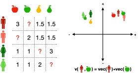
Figure 1: Two abstraction methods that can be used together to reduce information and computational constraints. Left: Low-rank matrix completion uses observed data to discover a latent vector for each item and buyer. Unobserved valuations are approximated using the dot product of these vectors. Right: Representative buyer/item abstractions collapse multiple buyers and/or multiple items into single representative agents.

Recall that most of the bounds (with exception of the Nash social welfare) related the quality of the equilibrium $(\hat{p},\hat{X})$ to $\|\Delta V\|_{1,\infty}$. This norm is computationally difficult to work with in practice since it is non-smooth. Instead, we will consider a much better understood matrix norm for practical applications, the Frobenius norm, which is defined as $\|\Delta V\|_{F}=(\sum_{i,j}\Delta v_{i,j}^{2})^{1/2}$.

Using the Frobenius norm implies that we have to settle for a less tight bound given by:

$$\|\Delta V\|_{1,\infty}=\max_{i\in[n]}\|\Delta v_{i}\|_{1}\leq\max_{i\in[n]}\sqrt{m}\|\Delta v_{i}\|_{2}\leq\sqrt{m}\|\Delta V\|_{F}.$$

Using the Frobenius norm gains us the ability to use well-known techniques to construct our abstractions. We will use low-rank matrix completion to learn missing entries and here it is well known that if $\hat{V}$ is the optimal $k$-rank approximation to $V$ then $\|\Delta V\|_{F}=(\sum_{i=k}^{\min(n,m)}\sigma^{2}_{i})^{1/2}$ where $\sigma_{i}$ is the $i^{th}$ singular value of the original matrix $V$—that is, the Frobenius norm is related to the ‘cut off’ singular values of the matrix.

Furthermore, if our matrix completion is being done from samples (as is common in many online applications) we can use a hold-out test set to estimate $\|\Delta V\|_{F}.$

In addition to rank-$k$ approximation, we will also use $k$-means clustering to reduce the size of $V$; this technique can also be viewed as a way of finding an approximation that minimizes the Frobenius norm (Bauckhage 2015).

Remark 1.

While our bound tells us about the quality of the allocations and prices, it tells us little about how close the values themselves are to the exact solution. It is known that the equilibrium $(p,X)$ is continuous in $V$ (Megiddo and Vazirani 2007). Thus, we can make the allocation and prices arbitrarily close by making $\|\Delta V\|$ sufficiently small. However, unlike quantities like regret, envy, etc., there is no linear relationship between $\|\Delta V\|$ and how far the abstracted price vector and allocation matrix is from the equilibrium under $V$. This is an interesting area for future work.

5.1 Low-Rank Matrix Completion

We begin with the information problem, that is, the case where not all entries of $V$ are known to us. Without some imputation of the missing entries, we cannot compute an equilibrium. If every $v_{ij}$ is completely independent and unpredictable from other valuations of the same buyer or other valuations of the same item by other buyers, then we have no hope of filling in missing entries in a sensible way. However, in most real world situations this is likely not the case and there is shared information across entries of the valuation matrix. To fill in the missing entries we can use standard techniques from matrix completion (e.g., Recht 2011).

A standard method for matrix completion is as follows: given a set of observations $\mathcal{O}$ of elements from a matrix $V$ with generic element $v_{ij}$, we try to find a set of vectors $vec(i)\in\mathbb{R}^{d}$ for every buyer $i$ and $vec(j)\in\mathbb{R}^{d}$ for every item $j$ to solve

$$\min_{vec}\sum_{v_{ij}\in\mathcal{O}}(v_{ij}-vec(i)\cdot vec(j))^{2}.$$

After we fit this model, we can construct a now complete matrix $\hat{V}$ of the original dimensionality with $\hat{v}_{ij}=vec(i)\cdot vec(j)$ and use this in place of $V$ for our task of interest. The solution ends up effectively minimizing $\min_{\hat{V}}\|V-\hat{V}\|_{F}$ over rank $d$ matrices $\hat{V}$. Note that matrix completion is not guaranteed to give positive $\hat{v}_{ij}$ even if all observed $v_{ij}$ are positive, so we replace all $\hat{v}_{ij}\leq.001$ with $.001.$

5.2 Representative Market Equilibrium

The issue of computation constraints when solving for market equilibrium arises because the EG program grows linearly in the size of the matrix $V$. This can lead to issues both with computation time, and especially memory usage. If an abstraction can reduce the number of buyers (and/or items), it can make the computation of equilibrium much more efficient. Given a valuation matrix $V$ we consider abstracting the market as follows.

5.2.1 Proportional Lift

Algorithm 1 Representative Market Equilibrium

Input: Set $\mathcal{O}$ of known valuations with generic element $o_{ij}$ (not necessarily the full matrix), $\hat{n}$, $\hat{m}$.

procedure Construct Representatives

     If matrix is fully available, use the row/columns as the vectors

     Else solve for vectors for each buyer $\text{vec}(i)$ and item $\text{vec}(j)$

     Use $k$-means clustering on the buyer vectors with $\hat{n}$ centroids

     Use $k$-means clustering on the item vectors with $\hat{m}$ centroids

     Use centroids of $k$-means as vector representations of representatives

     Set representative market valuations as dot products of above vectors

procedure Compute Representative Supplies/Budgets

     Sum budgets of buyers assigned to representative $i$ by $k$-means to get budget

     Sum supplies of items assigned to representative $j$ by $k$-means to get supply

Compute market equilibrium in the representative market

Algorithm 1 constructs a representative market equilibrium (RME) which we denote as $(\tilde{p}_{rep},\tilde{X}_{rep})$. The RME is of a different dimension than the original market. The question is now how to lift the prices and allocations to the original items and buyers. Prices are simple, we can just assign to every item $j$ the price of its representative item from the RME.

Allocations are more difficult. We first consider a proportional lift. We perform the lift in two steps. First we begin with $\tilde{X}_{rep}$ and construct a new allocation $X^{\prime}$ of dimension $\hat{n}\times m$ with $x^{\prime}_{i}$ being the allocation of original items to each representative buyer. Each representative buyer receives a supply weighted share of each item. Let $r(j)$ be the representative item for real item $j$. Then the amount of item $j$ that is allocated to representative buyer $i$ in this step is

$$x^{\prime}_{ij}=\dfrac{s_{j}}{\sum_{k\in r(j)}s_{k}}\tilde{x}_{ir(j)}.$$

Given $X^{\prime}$ we finish the lift by now splitting items across individuals proportionally to their budget. We denote the final allocation as $\hat{X}\in\mathbb{R}_{+}^{n\times m}$. Let $r(i)$ denote the representative buyer for real buyer $i$. The allocation of item $j$ to real buyer $i$ is

$$\hat{x}_{ij}=\dfrac{b_{i}}{\sum_{k\in r(i)}b_{k}}x^{\prime}_{r(i)j}.$$

Because everything is allocated proportionally we have that the supply constraint binds and thus the allocation is a full allocation. The proportional lift has the advantage that it is simple to compute and that our bounds can be applied directly. The allocations from the proportional RME are equivalent to those which would result if we constructed an approximate valuation matrix $\hat{V}$ by getting vector representations for each buyer/item, getting their representative abstraction, and replacing $v_{ij}$ by $\text{vec}(r(i))\cdot\text{vec}(r(j)).$

5.2.2 Recursive Lift

Proportional lifting is arguably the most direct and natural way to lift a solution. However, it makes no attempt to utilize the fact that the different buyers mapping to a single representative buyer are generally heterogeneous, even if similar. Next we present a lifting procedure which exploits the heterogeneity within each group of buyers assigned to the same representative buyer to improve on proportional lifting.

First, let us define $X^{R}$ to be an allocation of original items to representative buyers. We define a lift $L(X^{R})$ to be an allocation to the original buyers such that they are only allocated items from their respective representative buyer. We let $L_{i}(X^{R})$ be the bundle of goods received by buyer $i$ in the lift. We denote by $r(\tilde{i})$ the set of buyers assigned to representative buyer $\tilde{i}$.

Definition 5.

$L(X^{R})$ is a local lift if for any representative buyer $\tilde{i}$, we have that $\sum_{i\in r(\tilde{i})}L_{i}(X^{R})\leq x^{R}_{\tilde{i}}$.

Secondly, we shall use the less formal restriction that a local lift should be computable using only $X^{R}$ and the set of valuations $\{v_{i}:i\in r(\tilde{i})\}$.

To be concrete, consider the following example:

Example 2.

There are three buyers and three items, all with supplies and budgets equal to one. A representative market is created with two buyers: $\{(1),(2,3)\}$ and two items: $\{(1),(2,3)\}$. So, the first buyer and item remain unabstracted, but the latter two buyers and items are merged into a single representative buyer and item. Now, say that the solution to the abstraction is to split each of the two abstracted items in half. Then, the proportional lift is for buyers $2$ and $3$ to receive $\frac{1}{4}$ of each of the three original items. A local lift on the abstracted buyer is any reallocation of the items such that buyers $2$ and $3$ receive at most half of each item in aggregate.

The concept of a local lift is natural when we want to consider using parallelization for the computation of the lift. Locality means that only information about the allocation a representative buyer received is used to compute the re-allocation to the buyers represented by the representative buyer. Thus, we can solve the main abstraction and then solve each component of the lift (defined by each representative buyer) in parallel without any message passing. The proportional lift is a local lift.

Recall that the original objective function for the EG equilibrium is the maximization of Nash social welfare. Thus, we now consider a lift which is optimal in the family of local lifts in the sense that it is the NSW-maximizing one.

The lift works as follows: For each representative buyer, we look at the allocation of original items to that representative buyer in the abstraction equilibrium, denote this by $\tilde{x}^{R}_{\tilde{i}}$. We then construct a new local market for each representative buyer $i$. The buyers in the local market are individuals in $r(\tilde{i})$, their budgets are their original budgets, and supplies are $\tilde{x}^{R}_{\tilde{i}}$.

The lift $L(X^{R})$ is the solution to

$$\max_{X}\left\{\sum_{i\in r(\tilde{i})}\log(v_{i}\cdot x_{i}):\sum_{i\in r(\tilde{i})}{x_{i}}\leq\tilde{x}^{R}_{\tilde{i}}\right\}.$$

This lift yields a market equilibrium in the local market. We call this approach recursive representative market equilibrium (RRME). From the way the lift is constructed it is obvious that a local lift maximizes Nash social welfare among all local lifts if and only if it is an RRME.

In Example 2, the RRME is constructed by creating a new market with buyers $2$ and $3$ in it, and where the supply of each item is $1/2$. Then, we lift their allocation by finding a market equilibrium allocation of this new market. More generally we would need to solve for multiple markets, but here there is only one representative buyer that represents multiple original buyers.

We can also show that RRME is guaranteed to improve on several metrics relative to the proportional lift: Pareto gap, regret, MMS gap, and NSW by Theorem 5. Intuitively, this is due to the utility guarantee provided by market equilibrium, which says that each buyer does better than their budget-proportional allocation of each item.

Theorem 6.

Let $(p,X)$ be a solution obtained from proportional allocation from solving a representative market instance. Let $(p,X^{R})$ be the solution obtained by applying RRME to $(p,X)$. The RRME solution leads to weakly lower Pareto gap, regret, and MMS gap, as well as weakly higher NSW.

Proof.

First we note the following simple fact which holds for any agent $i$: the utility of $i$ under $X^{R}$ is weakly greater than that under $X$, i.e., $v_{i}\cdot x^{R}_{i}\geq v_{i}\cdot x_{i}$. This is because (a subset of) $X^{R}$ is a market equilibrium in the recursive market for the corresponding $\tilde{i}$, and an agent is guaranteed to get at least the value of the budget-proportional allocation in any market equilibrium.

The Pareto gap is the value of a linear program that maximizes social welfare (minus current welfare) subject to the constraint that each agent is weakly better off. Since utilities are greater in $X^{R}$ this is a strictly more constrained problem than for $X$, and thus the value, i.e., the Pareto gap, is lower.

Since we keep prices the same the optimal bundle $x_{i}^{*}$ for each agent remains the same for $(p,X)$ and $(p,X^{R})$. Thus the only affected part of regret is the negative term, which is weakly greater under $X^{R}$ since utilities are weakly greater.

That the MMS gap is smaller and NSW greater follows directly from each agent having weakly-higher utility. ∎

While the objectives in Theorem 6 are all guaranteed to improve in the RRME over the proportional lift, the example below shows that envy may not. Intuitively, this is because we may have an agent $i$ who does not envy agent $j$ very much in the proportional lift, but in the RRME $j$ improves very much while $i$ improves very little, thus generating an increase in envy.

Example 3.

Consider a 5-buyer-4-item instance with valuations $v_{1}=v_{2}=[1.5,1.5,0,0],v_{3}=[0,0,1+\epsilon,1-\epsilon],v_{4}=[0,0,1-\epsilon,1+\epsilon],v_{5}=[1.5,1.5,1+\epsilon,1-\epsilon]$, and budgets and supplies equal to $1$. Now consider the abstraction where buyers $1,2,5$ are clustered to a representative buyer with valuation $v_{\tilde{1}}=[1.5,1.5,0,0]$ and budget $3$, and buyers $3,4$ are clustered to a representative buyer with valuation $v_{\tilde{2}}=[0,0,1.5,1.5]$ and budget $2$. The representative market equilibrium with equal rates is to assign representative buyer $\tilde{1}$ all of items $1$ and $2$, each with price $1.5$ and assign representative buyer $\tilde{2}$ all of $3$ and $4$ at price $1$ each. This assignment leads to no envy when we perform the budget-proportional allocation. However, if we apply RME to representative buyer $\tilde{2}$ then buyers $3$ and $4$ get assigned all of items $3$ and $4$, respectively. Now buyer $5$ envies buyer $3$, as they could get $\epsilon$ more utility.

We view the potential increase in envy as a necessary price to pay in order to reap the benefits of locally optimizing each of the representative allocations. In order to avoid potential envy increases, we would need to take into account agents $i\notin r(\tilde{i})$ when computing the lift, which would often not be feasible computationally (since the whole point of the representative abstraction was to avoid a convex program whose size is on the order of $n\times m$).

6 Experimental Evaluation

6.1 First-Order Methods for Market Equilibrium

We initially considered solving the EG convex program directly via the CVXPY package (Diamond and Boyd 2016, Akshay Agrawal and Boyd 2018), which is a package for formulating convex programs in a uniform way, while utilizing underlying optimization solvers such as ECOS (Domahidi et al. 2013), CVXOPT (Andersen et al. 2013), and SCS (O’Donoghue et al. 2016). However, this approach turned out to have numerical problems once the number of agents and items reached around 130 each, regardless of the underlying solver.

To deal with those scalability issues, we solve the EG convex program via first-order methods. We consider the following Lagrangian relaxation:

$$\min_{0\leq p\leq\|B\|_{1}/s}\sum_{i\in[n]}\max_{0\leq x_{i}\leq s}B_{i}\log(v_{i}\cdot x_{i})-x_{i}\cdot p+s\cdot p\,.$$ (3)

This formulation allows us to apply standard algorithms for solving convex-concave saddle-point problems such as the primal-dual algorithm of Chambolle and Pock (2011, 2016) (henceforth referred to as PD). PD is an algorithm for solving problems of the following form (we omit some unnecessary generality):

$$\min_{x\in\cal X}\max_{p\in P}\ \mathcal{L}(x,p)\coloneqq x^{T}Kp+f(x)+s\cdot p$$ (4)

where $K$ is a matrix with bounded norm $L=\|K\|=\max_{\|x\|\leq 1,\|p\|\leq 1}\ x^{T}Kp$, and $f$ is a proper, lower semicontinuous convex function with a Lipschitz-bounded gradient, i.e., $\|\nabla f(x)-\nabla f(x^{\prime})\|\leq L_{f}\|x-x^{\prime}\|$ for all $x,x^{\prime}\in\cal X$.

An iteration of PD is as follows:

$$(\hat{p},\hat{X})= \mathcal{PD}_{\tau,\sigma}(\bar{x},\bar{p},\tilde{x},\tilde{p})\text{ where }$$

$$\begin{cases}\hat{x}=\arg\min_{x\in\cal X}f(\bar{x})+\langle\nabla f(\bar{x}),x-\bar{x}\rangle+x^{T}K\tilde{p}+\frac{1}{\tau}\|x-\bar{x}\|\,,\\ \hat{p}=\arg\min_{p\in P}\frac{1}{\sigma}\|x-\bar{x}\|-\tilde{x}^{T}Kp\,.\end{cases}$$

The algorithm repeatedly calls $\mathcal{PD}$ to generate a sequence of iterates as follows (note that the function invocation depends on the computed value, this is implementable because $x^{t+1}$ is computed before $p^{t+1}$):

$$(x^{t+1},p^{t+1})=\mathcal{PD}_{\tau,\sigma}(x^{t},p^{t},2x^{t+1}-x^{t},p^{t}).$$

The average iterates $\bar{x}=\sum_{t=1}^{T}x^{t}$ and $\bar{p}=\sum_{t=1}^{T}p^{t}$ converge to a saddle-point solution. The performance of the algorithm is usually measured in terms of reducing the saddle-point residual: $\max_{p}\mathcal{L}(\bar{x},p)-\min_{x}\mathcal{L}(x,\bar{p})$. A natural question is how quickly this error measure is driven to zero.

Nesterov and Shikhman (2018) study a formulation similar to (3), but where prices are unbounded, and they arrive at an algorithm where the saddle-point residual goes to zero at a rate of $O(1/\sqrt{T})$, but achieve additional auction-like properties in terms of the resulting dynamics. Leveraging the structure of our problem gives us even better worst-case bounds on convergence. Because in practice such worst case bounds are rarely reached and because these theoretical results are not the primary focus of our paper we discuss them informally here for completeness and relegate the formal statements to the Appendix:

Result 2.

Under mild assumptions the PD algorithm reduces the saddle-point residual of the EG problem at a rate of $O\left(\frac{n^{7/2}m^{2}}{T}\right)$.

The expression above makes some simplifying assumptions for readability. We include the full treatment in the Appendix. From the perspective of abstraction, the most important thing is that we have a $O(n^{7/2}m^{2})$ dependence on problem size. For this simplified rate we can give a nice expression for the savings in worst-case convergence rate due to our representative buyer/item abstraction:

Result 3.

Let $n$, $m$ be the number of buyers/items in the original market and $\hat{n}$, $\hat{m}$ be the number in the abstracted market. Under mild assumptions the representative buyer/item abstraction with proportional lift has a worst case convergence rate that is $O(\frac{\hat{n}^{7/2}\hat{m}^{2}}{n^{7/2}m^{2}})$ of the convergence rate of the full problem. If we use the recursive lift instead the relevant speedup is $O(\frac{\hat{n}^{5/2}\hat{m}^{2}}{n^{5/2}m^{2}}).$

While asymptotic analysis does not tell the whole story, the results do suggest that we should expect larger savings in computational complexity for ‘long and thin’ markets (those with many buyers and relatively few items) than those with many items and few buyers, which is precisely what we see in our experiments.

In practice, the primary concern is the memory usage of PD, as well as the cost per iteration. For the optimization formulation that uses PD, a variable is needed for every buyer and item pair, and thus memory usage is linear in the market size. Similarly, each step of PD can be computed in linear time for our setting. In practice, we thus get an asymptotic linear improvement to both memory usage and cost per iteration. In theory, we get much more than a linear improvement in total running time, based on the above estimates of the number of iterations needed in the worst case. However, in practice the number of iterations needed does not seem to grow much with the size of the market, and so the primary practical savings are those due to the memory and cost-per-iteration improvements.

In extremely large cases (e.g., online ad systems with millions of buyers and billions of impressions) it would not even be feasible to run PD on the original problem instance (typically due to memory usage), and so abstracting down to a manageable size becomes compulsory.

6.2 General Analysis Plan

We now evaluate the abstraction approaches above on several real datasets. We first discuss the analyses we perform on all datasets then we discuss each dataset in detail and give results.

For each dataset we compute the EG equilibrium in the full market and compare to the prices/allocations we generate using abstractions. We set budgets to $1$ and supplies to be such that there is one item per person (note that since we are in the divisible case, this only affects the prices/allocations up to a scaling factor).

We vary three properties of abstractions jointly. First, we replace the valuation matrix $V$ with a rank $k$ approximation for various $k$. To compute these low-rank representations we use the singular value decomposition (SVD). Second, we consider compressing the large number of buyers into a smaller set of representative buyers. We refer to this as abstraction coarseness and measure it as a percentage of the original market size. Thus, a $40\%$ abstraction is one which replaces 7200 original buyers with 2880 representative buyers via the $k$-means procedure above. Third, we compare the use of a proportional split and the recursive splitting. The goods were not abstracted in the first two datasets (but see Section 6.5 where we do abstract both sides).

In the results reported here we replace abstracted valuations (e.g., low-rank estimated ones) that are below $0$ with $0.01.$ This means that we do not allow our abstractions to turn any player into a ‘dummy player’ that receives no items.

We measure all of our theoretical quantities of interest: regret of each individual given each allocation (we normalize this by the maximum utility of the allocation), an individual’s envy (again, normalized by the utility that an individual would receive from the envied bundle), Nash social welfare (normalized by the Nash social welfare of the unabstracted market), Pareto optimality (normalized by the utility in the Pareto-optimal allocation), maximin share (normalized by utility being achieved).

We also look at one quantity for which we do not have bounds: total welfare/efficiency of the allocation (normalized by the total welfare of the unabstracted market). Note that market equilibrium makes no pretense of maximizing efficiency (indeed it only guarantees Pareto optimality and, in the case of EG equilibrium, Nash social welfare).

6.3 Dataset: Jester1

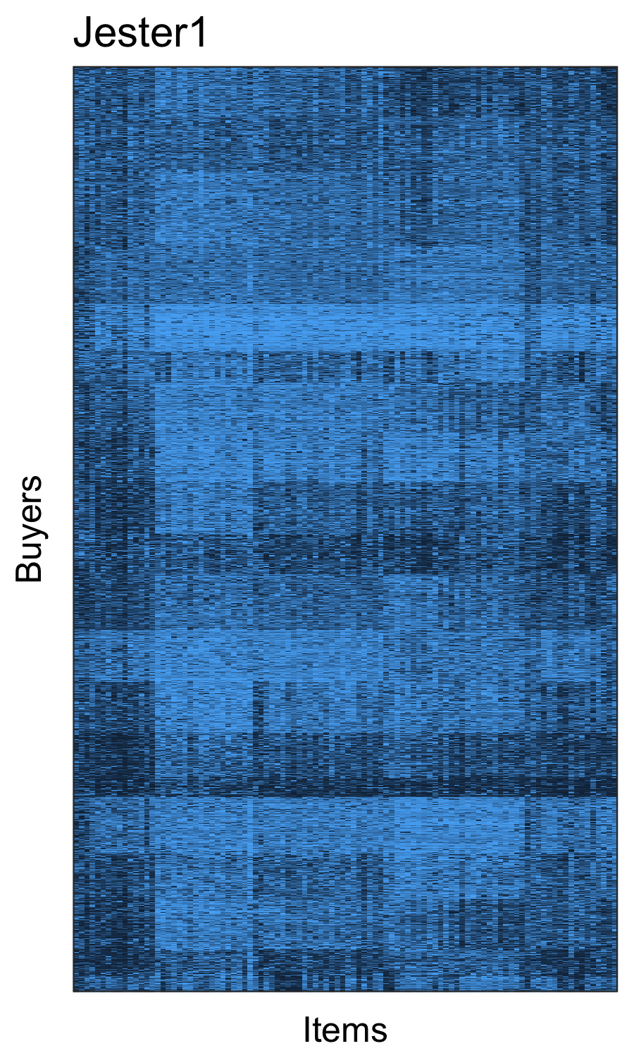
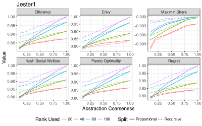
Figure 2: Market created by using valuation matrix from the Jester1 dataset with 7200 buyers and 100 items (left panel). There is clear structure suggesting compressibility. In this experiment we apply representative buyer abstraction only. Equilibria computed in quite coarse abstractions maintain good properties (right panel).

We begin by considering an existing dataset used for the evaluation of recommender systems. In typical recommender system datasets individuals give a rating (rather than a monetary evaluation) for each object. Nevertheless, standard recommender system datasets are still useful examples of valuation matrices for two reasons: first, when equilibrium computation is used for market design/fair division (e.g., CEEI and related algorithms at Wharton or Spliddit) the budget given to each individual is only virtual currency and, second, allocations in EG equilibrium are not affected by the scaling of an individual’s utilities so they are relatively robust to different ways individuals may interpret ratings.

The first dataset we consider, Jester 1, contains the evaluation of 100 jokes by over 79,000 individuals (Goldberg et al. 2001). We extract a submatrix of 7200 individuals that have rated all of the jokes giving us a complete market. Ratings in Jester are on a continuous scale between $-10$ and $10$ and our theory requires positive valuations so we shift the valuations to be (weakly) positive by shifting the whole matrix by $+10$.

Figure 2 left panel shows a representation of the Jester1 valuation matrix with lighter colors representing higher valuation. To show the structure more clearly we normalize each individual’s valuations to lie in $[0,1]$ for the figure (not the experiments) and perform clustering on the rows and columns to set the order they will be displayed. There is clear block structure suggesting that we can abstract the market using the representative buyer method effectively.

The right panel shows our main results. Even a coarse abstraction with recursion (720 representative buyers for 7200 original buyers and 20% rank compression) can yield an allocation that achieves almost $90\%$ of the Nash social welfare and efficiency of the unabstracted allocation and is almost Pareto optimal (there exists an allocation that improves total utility by 10% without leaving anyone worse off). Individuals display some regret (the abstracted allocation achieves $85\%$ of the utility they could achieve if buyers optimized given the abstraction prices) and some envy. Finally, we see that a weak notion of fair division, maximin share, is almost completely guaranteed under even the coarsest abstraction.

6.4 Dataset: Household Items

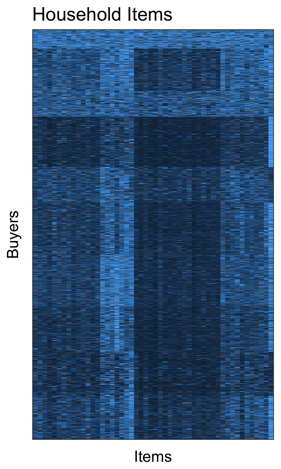
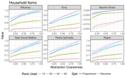
Figure 3: Market created by using a valuation matrix from the Household Item dataset with 2876 buyers and 50 items (left panel). There is clear structure suggesting compressibility. In this experiment we apply representative buyer abstraction only. Equilibria computed in quite coarse abstractions maintain good properties (right panel).

We also construct a new dataset of individuals who estimated their willingness-to-pay for 50 household items selected from a well-regarded online review site. Unlike in typical recommender datasets where items can often be naturally clustered into ‘types’ (e.g., romance movies, horror movies) we specifically chose items to span a broad range of product categories. (Examples: rain jacket, tool box, toaster, shovel, bluetooth headphones, thermos, blackout shade, bike pump, etc; see Figure 4 for full list of items and average valuations for each one.) Items were chosen to be representative of a large number of categories to make our compression problem more difficult.

In a survey conducted on an online labor market, individuals from the US were presented with a photo and brief description of each item. To deal with quality issues, specific brands and models for each item were selected from an online review site to be the ‘best in their class’ and participants were informed of this. Items were presented in a random order and participants entered their personal US dollar valuation for each item. At the end of the survey, participants were asked how well they felt they understood the questions/task. We use data from the 2876 individuals (out of 3300) that said they felt the task was natural and they could give a good personal valuation for all of the items. Here we list the items we used as well as their average valuations by individuals.

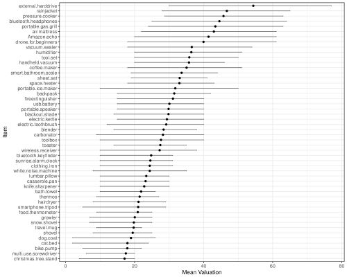
Figure 4: Items used in household item survey as well as their average valuations and first and third quantiles.

For this computational experiment, we apply matrix approximation, representative buyer/item modeling, and recursive reallocation.

Figure 3 shows the market, represented as in the Jester1 experiment above (left panel) as well as our main results (right panel). We see that even coarse abstractions can yield good properties and that recursive allocation meaningfully improves Pareto optimality and Nash social welfare of the approximations. There is a sharper tradeoff between compression and abstraction performance than in Jester. Recall though that this is because our candidate items were specifically chosen to be of quite different types and so display lower inter/intra item correlations in valuation than typical recommender datasets of, e.g., jokes or movies.

6.5 Dataset: MovieLens

Both datasets above includes many more buyers than items. We would like to consider a dataset where both sides of the market are large. However, asking individuals to evaluate many hundreds of items would be expensive and likely yield low quality data. Instead, we construct such a market from MovieLens 1M (Harper and Konstan 2015), a standard dataset for the evaluation of matrix completion algorithms. This dataset contains 6040 individuals with their ratings for a selection of 3952 total movies. In total, the dataset includes 1 million ratings. We treat each 1-5 rating as a valuation.

MovieLens 1M is very sparse (only a small percentage of possible user/movie rating pairs are observed) so we cannot use the data directly to construct a market as we could in the other datasets.

Instead, we will construct a semi-synthetic dataset by using the data to fit a low-rank approximation to the true rating matrix and doing our analysis on this model. We consider the submatrix which consists of the 1500 movies with the most observed ratings (avg. number of ratings: 579) and the top 1500 users who have rated the most movies (avg. number of ratings: 425). We use this submatrix as our valuation matrix for the market (Figure 5 left panel shows the market).

To generate the complete submatrix for the MovieLens 1M market we take the observed ratings denoted as $\mathcal{O}$ with generic element $o_{ij}$. We use PyTorch (Paszke et al. 2017) and minimize the loss function

$$\sum_{o_{ij}\in\mathcal{O}}(o_{ij}-\text{vec}(user_{i})\cdot\text{vec}(movie_{j})+\text{bias}(user_{i})+\text{bias}(movie_{j}))^{2}$$

over $d$ dimensional vectors for each user and movie and $1$ dimensional biases for each user and movie. We randomly split the data into an $80\%$ training set and a $20\%$ validation set and use the validation set to choose $d$ from the set $\{20,30,50,70,100\}$ and the weight decay parameter from the set $\{10^{-5},10^{-4},10^{-3},10^{-2},10^{-1}\}.$ We choose the best performing hyper-parameters from this group via the validation set (d=$20$, weight decay=$10^{-5}$).

We do not do any extensive tuning nor consider ‘proper’ test set accuracy as we are simply using this model to construct a simple semi-synthetic dataset for our experiment rather than trying to achieve state of the art prediction results.

Because the completion method already uses a low-rank approximation and because we cannot get the ground truth market equilibrium we only test the representative buyer abstraction here. Unlike in the datasets above, we construct both representative buyers and representative items. The right panel of Figure 5 shows that in this case even an extremely coarse abstraction (150 representative buyers, 150 representative items instead of the original 1500) can achieve outcomes that are quite close those of the full equilibrium.

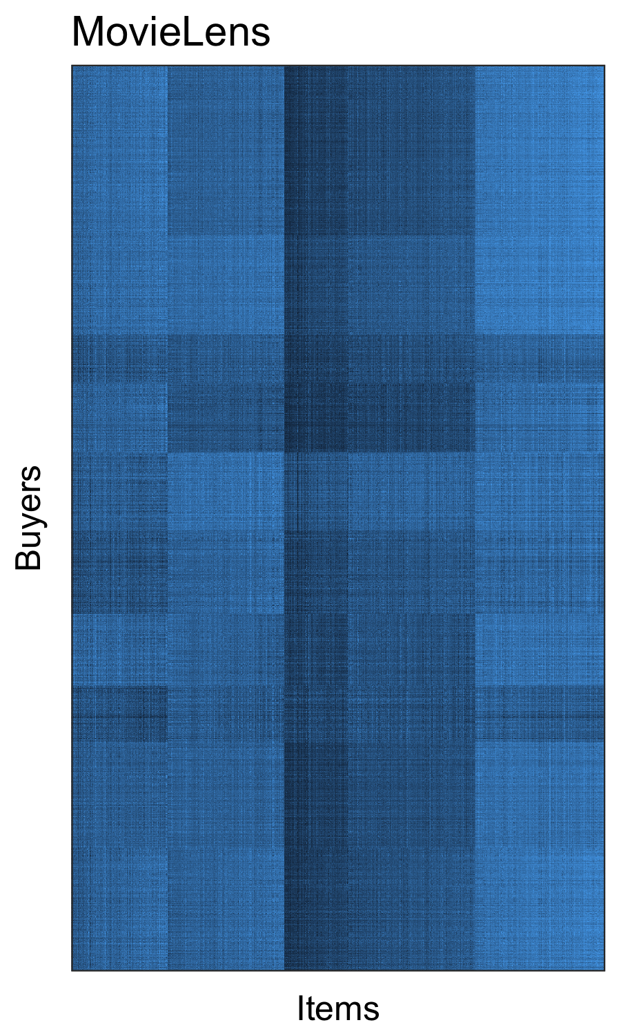
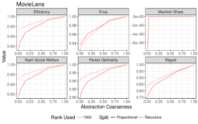
Figure 5: Market created by using valuation matrix from the MovieLens dataset with 1500 buyers and 1500 items (left panel). There is clear structure suggesting compressibility. In this experiment we apply both representative buyer and representative item abstraction. Equilibria computed in quite coarse abstractions maintain good properties (right panel).

6.6 A Large Market

In each of the experiments above, we used markets where we could compute the equilibrium for the full instance. We now consider an experiment for a market that is too large for us to compute the equilibrium for the full instance. In this case we cannot compute metrics like the NSW loss or the Pareto gap but we can still compute individual-level metrics like envy and regret.

As a large dataset we consider the larger MovieLens 10 million dataset. Here $69,897$ users rate $8228$ movies, for a total of $\sim 10$ million ratings. We construct the valuation vectors as in the smaller MovieLens markets above except using a $100$ dimensional embedding.

This problem is too large to solve the full instance on our commodity hardware. Instead, we solve a $4,000\times 4000$ abstraction—this is a more than $97\%$ reduction in size from the full market. We compute the allocations using both the proportional and recursive lifts.

Figure 6 shows the results of sampling $1,000$ buyers and computing their envy and regret associated with the lifted allocations and prices. We attain average regret near $16\%$ for the proportional lift and $14\%$ for the recursive lift, and correspondingly small average envy values. The worst values of regret and envy are not much higher.

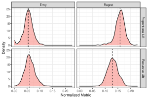
Figure 6: In the large MovieLens market, we cannot solve for the full equilibrium, however, we can compute individual levels of regret and envy for some sampled buyers. We see that a $97\%$ reduction in problem size is associated with a relatively small regret and envy in both the proportional and recursive lifts.

6.7 Quasi-Linear Markets

So far we have focused on the case where budgets are useless outside the market. This is the setting of interest for market designers that are using equilibrium as a tool for fair division of items (e.g., CEEI) and also marketing managers in ads marketplaces. However, our approximation results are also applicable to quasi-linear Fisher markets—those where leftover budget has use outside the market. In our household items dataset (unlike in Jester and MovieLens) individual valuations are given in dollars. Although quasi-linear valuations are not the main focus of this work, we present a preliminary experiment to investigate whether abstractions are useful in a quasi-linear market.

We use the same household items setup as above but now we consider quasi-linear utility and give each individual a budget of $\$10$. The quasi-linear case is slightly different from the standard one in several other ways. First, we know that there exists an equilibrium that can be found via a convex program but that this program no longer maximizes Nash social welfare. Second, doing a recursive lift generates multiple prices per item (different prices within each cluster) and is thus not interpretable anymore. Thus, we do not look at either of these in this experiment.

In addition, because now money is ‘real’ rather than existing solely for the sake of the mechanism, now we also consider an additional metric of interest: how well abstraction prices match up with true equilibrium prices. To measure this we consider the normalized price accuracy given by

$$1-\dfrac{\sum_{j}(\hat{p}_{j}-p_{j})^{2}}{\sum_{j}p_{j}^{2}}.$$

A value of $1$ means prices are perfectly predicted. It is known that prices are continuous in the $V$ matrix, so for a given desired level of price accuracy there exists a sufficiently small $\Delta V$ that attains that level. However, like efficiency or weak Pareto optimality, prices are not an LQFS and thus we have no formal guarantees about their accuracy when $\Delta V$ is not small.

Figure 7 show our main results. As with the standard Fisher case, we see that even coarse abstractions lead to fairly good results.

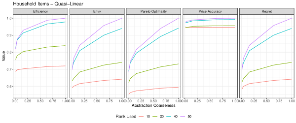
Figure 7: Quasi-linear Equilibria computed in quite coarse abstractions maintain good properties.

7 Conclusion and Future Directions

Computing market equilibria is a difficult problem. We have shown that the method of abstraction—solving a coarser problem and lifting the solution—can be used to reduce the information requirements and computation requirements of equilibrium computation. In addition, we have introduced a new dataset that we hope others can use for work on fair division.

There are many future directions to expand this research. In this work we looked at Fisher markets which assume additive valuations. This rules out situations where goods can be complements or substitutes. In the case of such preferences the information required to compute a market equilibrium becomes extremely large as we need to know the valuations of individuals for every possible combination of goods (Porter et al. 2003). However, recent work has begun to explore representing preferences with complements and substitutes in low-rank vector format (Ruiz et al. 2020, Peysakhovich and Ugander 2017). An interesting future direction is combining such techniques with abstraction methods. Generalizing beyond linear valuations could lead to greater scalability for problems such as public decision making, which have recently been related to market equilibria (Garg et al. 2020). Another interesting direction would be to apply abstraction techniques to more general market equilibrium problems under utilitarian welfare maximization.

A problem related to our setting is the cake cutting problem, where the goal is to allocate (WLOG) the interval $[0,1]$ to agents with heterogeneous preferences over subsets of the interval (Edmonds and Pruhs 2011, Chen et al. 2013, Balkanski et al. 2014, Aziz and Mackenzie 2016). This setting is significantly more complicated than linear Fisher markets. It would be interesting to investigate how our abstraction approach can be generalized to this harder setting, although the relationship to matrix decomposition becomes less pronounced. Some variants of cake cutting can be related directly to Fisher markets. Aziz and Ye (2014) show that cake cutting with piecewise-constant utilities is equivalent to linear Fisher market equilibrium, and Gao and Kroer (2021) show that general piecewise-linear utilities in cake cutting can be handled via Fisher markets with a continuum of items. The results of Aziz and Ye (2014) imply that our results extend directly to piecewise-constant-utility cake cutting, An interesting research direction is to what extent our results can be used to extended to other cake-cutting settings, for example via the relationship established by Gao and Kroer (2021).

We considered the use of market equilibria as allocation mechanisms (as in, e.g., the literature on fair division). However, another important use of computation of market equilibria is counterfactual estimation as in structural models in economics (Berry et al. 1995, Chawla et al. 2017). For example, an online marketplace may want to know how prices (and thus revenues) would change if certain market conditions (e.g., supplies, budgets) were to change. Using the method of abstracting large markets to answer such questions is also an important future direction.

We looked at two methods that could be jointly used to create abstractions: low-rank approximation and representative buyer/item modeling. The representative market abstraction speeds up computation but we did not use low-rank structure for anything but filling in missing data. An interesting algorithmic question is whether the low-rank structure can be leveraged to speed up the gradient calculation steps of our first-order methods, for example, by employing recent techniques for fast nearest neighbor search (Johnson et al. 2019).

Our work fits into the nascent but growing literature on combining techniques from machine learning/AI with classical results from game theory to solve market design (Feng et al. 2018, Golowich et al. 2018), game abstraction (Moravčík et al. 2017, Brown et al. 2019), and agent design (Lerer and Peysakhovich 2017, 2019) problems that cannot be easily solved in closed form. In this work we leveraged standard linear abstractions (low-rank approximation, k-means clustering). A question for future work is whether more complex, non-linear methods, can be used to construct even better abstractions.

8 Author Biographies

Christian Kroer

Christian Kroer is an Assistant Professor of Industrial Engineering and Operations Research at Columbia University, as well as a member of the Data Science Institute at Columbia. His research interests are at the intersection of operations research, economics, and computation, with a focus on how optimization and AI methods enable large-scale economic solution concepts. He obtained his Ph.D. in computer science from Carnegie Mellon University, and spent a year as a postdoc with the Economics and Computation team at Facebook Research. He was a winner of the 2016-2018 Facebook Fellowship in economics and computation, and a runner-up in the 2017 INFORMS Computing Society Student Paper Competition.

Alexander Peysakhovich

Alexander Peysakhovich is a senior research scientist at Facebook Artificial Intelligence research. His work includes both basic and applied research at the intersection of behavioral science, economics, game theory, and artificial intelligence. He holds a PhD in Behavioral Economics from Harvard."

Eric Sodomka

Eric Sodomka is a Research Scientist on the Core Data Science team at Facebook, as well as an advisory board member of Data Science Nigeria. His research interests lie at the intersection of economics and computer science. In particular, he is interested in designing markets that facilitate collaboration across academic disciplines, that connect theoreticians and practitioners, and that improve opportunities for underrepresented groups. He currently resides in Edinburgh, Scotland. Prior to that, he worked in Facebook’s Menlo Park office, where he managed the Algorithmic Game Theory and Market Design Research group. He received his Ph.D. in Computer Science from Brown University.

Nicolas Stier-Moses

Nicolas Stier-Moses is a Director at Facebook Core Data Science. His work leverages innovative research to drive impact to the products, infrastructure and processes at Facebook, the company. The group draws inspiration from a rich and diverse set of disciplines including Operations, Economics, Mechanism Design, Algorithms, Statistics, Machine Learning, Experimentation, and Computational Social Science. Between 2014 and 2017, he supported the Economics, Algorithms and Optimization team, which is one of the areas of focus of Core Data Science. Prior to joining Facebook, Nicolas was an Associate Professor at the Decision, Risk and Operations Division of Columbia Business School and at the Business School of Universidad Torcuato Di Tella. He received a Ph.D. degree from the Operations Research Center at the Massachusetts Institute of Technology.

Appendix A Appendix

A.1 Linear properties

Balkanski et al. (2014) defined linear properties as properties of allocations that can be represented as an index set $G$ of finitely-many linear constraints:

$$\sum_{i,j}A^{k}_{ij}u_{i}(x_{j})\geq c^{k}\quad\forall k\in G$$

such that $\sum_{ij}A^{k}_{ij}\leq 1$ for all $k\in G$. It is easy to show that linear properties are approximately preserved under $\hat{V}$. Here $G$ is allowed to be an arbitrary finite-sized index set of constraints (so for example, $G$ could be the set of inequalities required for no envy).

Consider any $k\in G$, we have:

$$c^{k} \leq\sum_{i,j}A^{k}_{ij}\hat{u}_{i}(x_{j})=\sum_{i,j}A^{k}_{ij}(u_{i}(x_{j})-\Delta v_{i}\cdot x_{j})=\sum_{i,j}A^{k}_{ij}u_{i}(x_{j})-\sum_{i,j}A^{k}_{ij}\Delta v_{i}\cdot x_{j}\leq\max_{i,j}\hat{u}_{i}(x_{j})$$

Now we can use the sum-to-less-than-one property of $A^{k}$ to bound the error:

$$\sum_{i,j}A^{k}_{ij}\Delta v_{i}\cdot x_{j}\leq\max_{i,j}\Delta v_{i}\cdot x_{j}\leq\max_{i}\|\Delta v_{i}\|_{1}=\|\Delta V\|_{1,\infty}$$

Thus we can use this general bound on linear properties to show that envy and equitability, as well as any other linear property, is preserved up to an additive error $\|\Delta V\|_{1,\infty}$. Balkanski et al. (2014) also mention proportionality as a linear property, however here one has to be slightly careful in our setting. Because we have two different market instances $V,V^{\prime}$, it is not generally the case that there exists a single set of linear-property constants $A,c$ representing proportionality as a linear constraint, since the $c$ is in general different for $V$ and $V^{\prime}$. Thus our result on MMS and proportionality being preserved does not follow directly from bounding linear properties. One has to further relate the RHS constants $c$ and $c^{\prime}$ under the two instances.

A.2 Proof of Theorem 1

Proof.

We first show the result for a per-buyer property. Let $X^{\prime}\in\mathcal{X}^{k}$, $i$ be any buyer for which the quantification holders under $\hat{V}$, $i^{\prime}$ be arbitrary, and $i^{\prime\prime}$ the minimizer of $u_{i}(x_{i^{\prime\prime}}^{\prime})$, we then have

$$\hat{u}_{i}(\hat{x}_{i})\geq\lambda_{1}^{k}\hat{u}_{i}(\hat{x}_{i^{\prime}})+\lambda_{2}^{k}\min_{i^{\prime}}\hat{u}_{i}(\hat{x}_{i^{\prime}}^{\prime})\Leftrightarrow\\ \sum_{j}\hat{v}_{ij}(\hat{x}_{ij}-\lambda_{1}^{k}\hat{x}_{i^{\prime}j}-\lambda_{2}^{k}x_{i^{\prime\prime}j}^{\prime})+QL(B_{i}-\hat{p}_{j}(\hat{x}_{i}-\lambda_{1}^{k}\hat{x}_{i^{\prime}}-\lambda_{2}^{k}x_{i^{\prime\prime}}^{\prime}))\geq 0,$$

where $QL\in\{0,1\}$ is a constant which denotes whether $u_{i}$ is quasilinear. This is equivalent to

$$\sum_{j}v_{ij}(\hat{x}_{ij}-\lambda_{1}^{k}\hat{x}_{i^{\prime}j}-\lambda_{2}^{k}x_{i^{\prime\prime}j}^{\prime})+QL(B_{i}-\hat{p}_{j}(\hat{x}_{i}-\lambda_{1}^{k}\hat{x}_{i^{\prime}}-\lambda_{2}^{k}x_{i^{\prime\prime}}^{\prime}))\geq-\sum_{j}\Delta v_{ij}(\hat{x}_{ij}-\lambda_{1}^{k}\hat{x}_{i^{\prime}j}-\lambda_{2}^{k}x_{i^{\prime\prime}j}^{\prime}).$$

We can rewrite this in terms of $u_{i}$ to get

$$u_{i}(\hat{x}_{i})-(\lambda_{1}^{k}u_{i}(\hat{x}_{i^{\prime}})+\lambda_{2}^{k}\min_{i^{\prime}}u_{i}(\hat{x}_{i^{\prime}}^{\prime})) \geq-\sum_{j}\Delta v_{ij}(\hat{x}_{ij}-\lambda_{1}^{k}\hat{x}_{i^{\prime}j}-\lambda_{2}^{k}x_{i^{\prime}j}^{\prime}),$$

$$\geq-\sum_{j}|\Delta v_{ij}|\max(\hat{x}_{ij},\lambda_{1}^{k}\hat{x}_{i^{\prime}j}+\lambda_{2}^{k}x_{i^{\prime}j}^{\prime}),$$

$$\geq-\|\Delta V\|_{1,\infty}\max(1,\lambda_{1}^{k}+\lambda_{2}^{k}).$$

Since $i^{\prime}$ was arbitrary this implies

$$u_{i}(\hat{x}_{i})-(\lambda_{1}^{k}\max_{i^{\prime}}u_{i}(\hat{x}_{i^{\prime}})+\lambda_{2}^{k}\min_{i^{\prime}}u_{i}(\hat{x}_{i^{\prime}}^{\prime}))\geq-\|\Delta V\|_{1,\infty}\max(1,\lambda_{1}^{k}+\lambda_{2}^{k}).$$

Thus the property holds approximately for buyer $i$ under $V$, as the theorem requires.

Now consider a global property $k$. By definition we have that for any alternative allocation $X^{\prime}\in\mathcal{X}^{k}$

$$0 \leq\sum_{i\in[n]}\beta_{i}\hat{v}_{i}\cdot\hat{x}_{i}-\sum_{i\in[n]}\beta_{i}\hat{v}_{i}\cdot\hat{x}^{\prime}_{i}$$

$$=\sum_{i\in[n]}\sum_{j\in[m]}\beta_{i}\hat{v}_{i}\cdot(\hat{x}_{i}-\hat{x}^{\prime}_{i})$$

$$=\sum_{i\in[n]}\sum_{j\in[m]}\beta_{i}(v_{i}-\Delta v_{i})\cdot(\hat{x}_{i}-\hat{x}^{\prime}_{i})$$

$$\leq\sum_{i\in[n]}\sum_{j\in[m]}\beta_{i}v_{i}\cdot(\hat{x}_{i}-\hat{x}^{\prime}_{i})+\sum_{i\in[n]}\sum_{j\in[m]}\beta_{i}\|\Delta v_{i}\|_{1}.$$

∎

A.3 Proofs of Other Theorems

Proof of Theorem 5: Bounded NSW.

We have

$$\text{NSW}(X^{*})=\prod_{i\in[n]}v_{i}\cdot x^{*}_{i}=\prod_{i\in[n]}(\hat{v}_{i}\cdot x^{*}_{i}+\Delta v_{i}\cdot x^{*}_{i})=\prod_{i\in[n]}\hat{v}_{i}\cdot x^{*}_{i}\bigg{(}1+\frac{\Delta v_{i}\cdot x^{*}_{i}}{\hat{v}_{i}\cdot x^{*}_{i}}\bigg{)}.$$

Now we can use the fact that $X^{*}$ is feasible under $\hat{V}$ to note that its value must be less than that of $\hat{X}$:

$$\text{NSW}(X^{*})\leq\prod_{i\in[n]}\hat{v}_{i}\cdot\hat{x}_{i}\bigg{(}1+\frac{\Delta v_{i}\cdot x^{*}_{i}}{\hat{v}_{i}\cdot x^{*}_{i}}\bigg{)}\leq\prod_{i\in[n]}\hat{v}_{i}\cdot\hat{x}_{i}\bigg{(}1+\frac{\|\Delta v_{i}\|_{1}}{\hat{v}_{i}\cdot x^{*}_{i}}\bigg{)}=\text{NSW}(\hat{X})\prod_{i\in[n]}\bigg{(}1+\frac{\|\Delta v_{i}\|_{1}}{\hat{v}_{i}\cdot x^{*}_{i}}\bigg{)}.$$

∎

Proof of Theorem 6: RRME weakly improves buyer utilities.

First we note the following simple fact which holds for any buyer $i$: the utility of $i$ under $X^{r}$ is weakly greater than that under $X$, i.e., $v_{i}\cdot x^{r}_{i}\geq v_{i}\cdot x_{i}$. This is because (a subset of) $X^{r}$ is a market equilibrium in the recursive market for the corresponding $\tilde{i}$, and a buyer is guaranteed to get at least the value of the budget-proportional allocation in any market equilibrium.

The Pareto gap is the value of a linear program that maximizes social welfare (minus current welfare) subject to the constraint that each buyer is weakly better off. Since utilities are greater in $X^{r}$ this is a strictly more constrained problem than for $X$, and thus the value, i.e., the Pareto gap, is lower.

Since we keep prices the same the optimal bundle $x_{i}^{*}$ for each buyer remains the same for $(p,X)$ and $(p,X^{r})$. Thus the only affected part of regret is the negative term, which is weakly greater under $X^{r}$ since utilities are weakly greater.

That the MMS gap is smaller and NSW greater follows directly from each buyer having weakly-higher utility. ∎

A.4 Convergence Rates of RME Computation

The average iterates $\bar{x}=\sum_{t=1}^{T}x^{t}$ and $\bar{p}=\sum_{t=1}^{T}p^{t}$ converge to a saddle-point solution at a rate of $O(\frac{(L+L_{f})D_{x}+LD_{p}}{T})$, where $D_{x},D_{p}$ is the maximum value of the $\ell_{2}$ norm over $\cal X$ and $P$ respectively. Note that we upper bound the price vector $p$ by the sum of budgets $\|B\|_{1}$, and each allocation vector $x_{i}$ by the supply of each item. This does not change the set of equilibria, as these conditions are all guaranteed to be satisfied in equilibrium.

We now show how to instantiate our SPP (3) in terms of the generic SPP (4). We have that $\cal X$ is the product of allocation vectors $\times_{i\in[n]}\{x_{i}:0\leq x_{i}\leq s\}$ over the buyers, and $P=\{p:0\leq p\leq\|B\|_{1}/s\}$ is the set of price vectors. $K$ is an $nm\times m$ matrix representing $\sum_{i\in[n]}p\cdot x_{i}$, i.e., with a $1$ in each row/column-pair $r,j$ when the row $r$ corresponds to a variable that denotes assigning item $j$ to some bidder. The norm $L$ of $K$ is $\sqrt{n}$, which is achieved by any pair $x,p$ such that $p_{j}=1$ for some $j$, and $x_{ij}=\frac{1}{\sqrt{n}}$, with all other entries $0$, or by setting $p=\frac{1}{\sqrt{m}},x=\frac{1}{\sqrt{mn}}$.

The logarithm in the objective function presents a challenge because the gradient is unbounded near zero; this problem can be addressed by noting that agents are always guaranteed to receive their MMS value in equilibrium, and thus we can add the additional constraint $v_{i}\cdot x_{i}\geq\textrm{MMS}_{i}$ to the feasible set of each agent, thereby bounding the gradient difference $L_{f}$ by $\max_{i\in[n],j\in[m]}\frac{v_{ij}B_{i}}{\textrm{MMS}_{i}}$. In practice we found that utilities did not approach zero and thus this projection was unnecessary.

The value of $D_{x}$ is $n\|s\|_{2}^{2}$, the maximum is achieved by setting $x_{ij}=s_{j}$ for all $i,j$. The value of $D_{p}$ is $\sum_{j\in[m]}(\|B\|_{1}/s_{j})^{2}$, the maximum is achieved by setting each price at its upper bound.

Putting together this construction gives an algorithm that converges to a saddle point of (3) at a rate of

$$\max_{p\in P}\mathcal{L}(\bar{x},p)-\min_{x\in\cal X}\mathcal{L}(x,\bar{p})\leq O\bigg{(}\frac{(\sqrt{n}+\max_{i,j}\frac{v_{ij}B_{i}}{\textrm{MMS}_{i}})n\|s\|_{2}^{2}+\sqrt{n}\sum_{j\in[m]}(\|B\|_{1}/s_{j})^{2}}{T}\bigg{)}.$$

Now we see that if we solve a clustering $(\{C_{\tilde{i}}\},\{C_{\tilde{j}}\})$ we get the following convergence rate:

$$O\bigg{(}\frac{(\sqrt{\hat{n}}+\max_{i\in[\hat{n}],j\in[\hat{m}]}\frac{\hat{v}_{ij}\hat{B}_{i}}{\textrm{MMS}_{i}})\hat{n}\|\hat{s}\|_{2}^{2}+\sqrt{\hat{n}}\sum_{j\in[\hat{m}]}(\|\hat{B}\|_{1}/\hat{s}_{j})^{2}}{T}\bigg{)}.$$ (5)

Furthermore, each iteration is of order $O(\hat{n}\hat{m})$ rather than $O(nm)$. To get a sense of the savings in running time, say that supply and budgets are both $1$. In that case the original problem has runtime cost $O(n^{7/2}m^{2})$ (since the third term usually dominates), and thus compressing to $10\%$ problem size leads to a runtime decrease of factor $100$ to $3162$ depending on whether the decrease in instance size is primarily due to fewer items or buyers.

If we apply recursive lift then we have to solve $k$ market equilibrium problems corresponding to each cluster of buyers. The cost of computing the recursive allocations is the sum of the costs of computing each recursive market equilibrium. This can be expressed as a sum over terms similar to (5), but where $\hat{n},\hat{m}$ represent the size of the given recursive instance. Again we assume that budgets and supplies are $1$ to get a sense of runtime savings. We can then use the fact that the union of the buyer clusters is $[n]$ to bound the runtime as $O(n\hat{n}^{5/2}\hat{m}^{2})$, where $\hat{n},\hat{m}$ corresponds to the size of the recursive market equilibrium which maximizes $\hat{n}^{5/2}\hat{m}^{2}$. Thus even with the additional cost of computing the RME allocation the runtime cost savings are on the order of $100$ to $316$ for the case where each recursive market is a tenth of the size of the original market.

A.5 Quasilinear variant

In this section we describe how our results can be instantiated for quasilinear (QL) utilities.

Each buyer $i$ has a utility that now depends on how much leftover money they have. We let $\delta_{i}$ denote the amount of leftover money. The utility of buyer $i$ is now

$$u_{i}^{QL}(x_{i},\delta_{i})=v_{i}\cdot x_{i}+\delta_{i}$$

.

Given prices $p\in\mathbb{R}_{+}^{m}$ for the goods, a QL demand for buyer $i$ is

$$d_{i}^{QL}(p)=\{\arg\max_{x,\delta:x\cdot p+\delta\leq B_{i}}v_{i}\cdot x+\delta\}.$$

The QL demand can be set valued but the maximum reachable utility given a price vector is unique.

Similar to the non-QL case, a market equilibrium can be computed via convex programming (EG-QL):

$$\underset{x}{\text{max}} \sum_{i}B_{i}\text{log}(v_{i}\cdot x_{i}+\delta_{i})-\delta_{i}$$

subject to $$\sum_{i}x_{ij}\leq s_{j}\text{ }\forall j$$

Note that this convex program is almost identical to the standard EG program; the only difference is the introduction of $\delta_{i}$ for each buyer $i$ (this convex program for QL utilities was first given by Chen et al. (2007) and later by Cole et al. (2017)).

Now consider the utility function $\hat{u}_{i}^{QL}(x_{i},\delta_{i})=\hat{v}_{i}\cdot x_{i}+\delta_{i}$. Since the $\delta_{i}$ term does not depend on $\hat{V}$, we have

$$u_{i}^{QL}(x_{i},\delta_{i})=v_{i}\cdot x_{i}+\delta_{i}=(\hat{v}_{i}+\Delta v_{i})\cdot x_{i}+\delta_{i}=\hat{u}_{i}^{QL}(x_{i},\delta_{i})+\Delta v_{i}\cdot x_{i},$$

and thus the abstracted utility function behaves exactly the same as in the non-QL case with respect to the abstraction error $\Delta v_{i}$. We then have that

Theorem 7.

Envy, regret, MMS, proportional share, and strong Pareto improvement are LQFS properties under QL utilities, and are thus bounded by $\|\Delta V\|_{1,\infty}$. Weighted social welfare is LQFS and is thus bounded by $\|\hat{w}\|_{1}\|\Delta V\|_{1,\infty}$ for weights $\hat{w}$.

The proof is identical to the non-QL case after noting that $\Delta v_{i}$ behaves exactly the same in both cases.

References

- Akshay Agrawal and Boyd (2018) Akshay Agrawal SD Robin Verschueren, Boyd S (2018) A rewriting system for convex optimization problems. Journal of Control and Decision 5(1):42–60.
- Andersen et al. (2013) Andersen M, Dahl J, Vandenberghe L (2013) Cvxopt: A Python package for convex optimization. http://abel.ee.ucla.edu/cvxopt . Last accessed April 2021.
- Azevedo and Budish (2018) Azevedo EM, Budish E (2018) Strategy-proofness in the large. The Review of Economic Studies 86(1):81–116.
- Aziz and Mackenzie (2016) Aziz H, Mackenzie S (2016) A discrete and bounded envy-free cake cutting protocol for any number of agents. Foundations of Computer Science (FOCS), 2016 IEEE 57th Annual Symposium on, 416–427 (IEEE).
- Aziz and Ye (2014) Aziz H, Ye C (2014) Cake cutting algorithms for piecewise constant and piecewise uniform valuations. International Conference on Web and Internet Economics, 1–14 (Springer).
- Baldwin and Klemperer (2019) Baldwin E, Klemperer P (2019) Understanding preferences: “demand types”, and the existence of equilibrium with indivisibilities. Econometrica 87(3):867–932.
- Balkanski et al. (2014) Balkanski E, Kurokawa D, Brânzei S, Procaccia AD (2014) Simultaneous cake cutting. Proceedings of the Twenty-Eighth AAAI Conference on Artificial Intelligence, 566–572, AAAI’14 (AAAI Press).
- Bauckhage (2015) Bauckhage C (2015) K-means clustering is matrix factorization. arXiv preprint arXiv:1512.07548 .
- Berry et al. (1995) Berry S, Levinsohn J, Pakes A (1995) Automobile prices in market equilibrium. Econometrica: Journal of the Econometric Society 841–890.
- Bhojanapalli et al. (2016) Bhojanapalli S, Neyshabur B, Srebro N (2016) Global optimality of local search for low rank matrix recovery. Advances in Neural Information Processing Systems, 3873–3881.
- Bichler et al. (2020) Bichler M, Fichtl M, Schwarz G (2020) Walrasian equilibria from an optimization perspective: A guide to the literature. Naval Research Logistics (NRL) .
- Bichler and Waldherr (2019) Bichler M, Waldherr S (2019) Computing core-stable outcomes in combinatorial exchanges with financially constrained bidders. Proceedings of the 2019 ACM Conference on Economics and Computation, 747–747.
- Birnbaum et al. (2011) Birnbaum B, Devanur NR, Xiao L (2011) Distributed algorithms via gradient descent for Fisher markets. Proceedings of the 12th ACM conference on Electronic commerce, 127–136 (ACM).
- Borgs et al. (2007) Borgs C, Chayes J, Immorlica N, Jain K, Etesami O, Mahdian M (2007) Dynamics of bid optimization in online advertisement auctions. Proceedings of the 16th international conference on World Wide Web, 531–540 (ACM).
- Bottou et al. (2013) Bottou L, Peters J, Quiñonero-Candela J, Charles DX, Chickering DM, Portugaly E, Ray D, Simard P, Snelson E (2013) Counterfactual reasoning and learning systems: The example of computational advertising. The Journal of Machine Learning Research 14(1):3207–3260.
- Brown et al. (2015) Brown N, Ganzfried S, Sandholm T (2015) Hierarchical abstraction, distributed equilibrium computation, and post-processing, with application to a champion no-limit texas hold’em agent. Proceedings of the 2015 International Conference on Autonomous Agents and Multiagent Systems, 7–15 (International Foundation for Autonomous Agents and Multiagent Systems).
- Brown et al. (2019) Brown N, Lerer A, Gross S, Sandholm T (2019) Deep counterfactual regret minimization. Chaudhuri K, Salakhutdinov R, eds., Proceedings of the 36th International Conference on Machine Learning, ICML 2019, 9-15 June 2019, Long Beach, California, USA, volume 97 of Proceedings of Machine Learning Research, 793–802 (PMLR).
- Brown and Sandholm (2018) Brown N, Sandholm T (2018) Superhuman ai for heads-up no-limit poker: Libratus beats top professionals. Science 359(6374):418–424.
- Budish (2011) Budish E (2011) The combinatorial assignment problem: Approximate competitive equilibrium from equal incomes. Journal of Political Economy 119(6):1061–1103.
- Budish et al. (2016) Budish E, Kessler JB, et al. (2016) Bringing Real Market Participants’ Real Preferences into the Lab: An Experiment that Changed the Course Allocation Mechanism at Wharton (National Bureau of Economic Research).
- Caragiannis et al. (2016) Caragiannis I, Kurokawa D, Moulin H, Procaccia AD, Shah N, Wang J (2016) The unreasonable fairness of maximum Nash welfare. Proceedings of the 2016 ACM Conference on Economics and Computation, 305–322 (ACM).
- Chambolle and Pock (2011) Chambolle A, Pock T (2011) A first-order primal-dual algorithm for convex problems with applications to imaging. Journal of mathematical imaging and vision 40(1):120–145.
- Chambolle and Pock (2016) Chambolle A, Pock T (2016) On the ergodic convergence rates of a first-order primal–dual algorithm. Mathematical Programming 159(1-2):253–287.
- Chawla et al. (2017) Chawla S, Hartline JD, Nekipelov D (2017) Mechanism redesign. arXiv preprint arXiv:1708.04699 .
- Chen et al. (2007) Chen L, Ye Y, Zhang J (2007) A note on equilibrium pricing as convex optimization. International Workshop on Web and Internet Economics, 7–16 (Springer).
- Chen et al. (2009) Chen X, Dai D, Du Y, Teng SH (2009) Settling the complexity of Arrow-Debreu equilibria in markets with additively separable utilities. 2009 50th Annual IEEE Symposium on Foundations of Computer Science, 273–282 (IEEE).
- Chen and Teng (2009) Chen X, Teng SH (2009) Spending is not easier than trading: on the computational equivalence of Fisher and Arrow-Debreu equilibria. International Symposium on Algorithms and Computation, 647–656 (Springer).
- Chen et al. (2013) Chen Y, Lai JK, Parkes DC, Procaccia AD (2013) Truth, justice, and cake cutting. Games and Economic Behavior 77(1):284–297.
- Cole et al. (2017) Cole R, Devanur NR, Gkatzelis V, Jain K, Mai T, Vazirani VV, Yazdanbod S (2017) Convex program duality, Fisher markets, and Nash social welfare. 18th ACM Conference on Economics and Computation, EC 2017 (Association for Computing Machinery, Inc).
- Cole and Gkatzelis (2018) Cole R, Gkatzelis V (2018) Approximating the Nash social welfare with indivisible items. SIAM Journal on Computing 47(3):1211–1236.
- Conitzer et al. (2019) Conitzer V, Kroer C, Panigrahi D, Schrijvers O, Sodomka E, Stier-Moses NE, Wilkens C (2019) Pacing equilibrium in first-price auction markets. Proceedings of the 2019 ACM Conference on Economics and Computation, 587, EC ’19 (New York, NY, USA: Association for Computing Machinery).
- Conitzer et al. (2021) Conitzer V, Kroer C, Sodomka E, Stier-Moses NE (2021) Multiplicative pacing equilibria in auction markets. Operations Research Forthcoming.
- Diamond and Boyd (2016) Diamond S, Boyd S (2016) CVXPY: A Python-embedded modeling language for convex optimization. Journal of Machine Learning Research 17(83):1–5.
- Domahidi et al. (2013) Domahidi A, Chu E, Boyd S (2013) ECOS: An SOCP solver for embedded systems. European Control Conference (ECC), 3071–3076.
- Edmonds and Pruhs (2011) Edmonds J, Pruhs K (2011) Cake cutting really is not a piece of cake. ACM Trans. Algorithms 7(4):51.
- Eisenberg and Gale (1959) Eisenberg E, Gale D (1959) Consensus of subjective probabilities: The pari-mutuel method. The Annals of Mathematical Statistics 30(1):165–168.
- Feng et al. (2018) Feng Z, Narasimhan H, Parkes DC (2018) Deep learning for revenue-optimal auctions with budgets. Proceedings of the 17th International Conference on Autonomous Agents and Multiagent Systems, 354–362 (International Foundation for Autonomous Agents and Multiagent Systems).
- Ganzfried and Sandholm (2014) Ganzfried S, Sandholm T (2014) Potential-aware imperfect-recall abstraction with earth mover’s distance in imperfect-information games. Proceedings of the Twenty-Eighth AAAI Conference on Artificial Intelligence, 682–690 (AAAI Press).
- Gao and Kroer (2021) Gao Y, Kroer C (2021) Infinite-dimensional Fisher markets: Equilibrium, duality and optimization. Proceedings of the AAAI Conference on Artificial Intelligence.
- Garg et al. (2020) Garg N, Goel A, Plaut B (2020) Markets for public decision-making. Social Choice and Welfare .
- Ge et al. (2016) Ge R, Lee JD, Ma T (2016) Matrix completion has no spurious local minimum. Advances in Neural Information Processing Systems, 2973–2981.
- Gilpin et al. (2007) Gilpin A, Sandholm T, Sørensen TB (2007) Potential-aware automated abstraction of sequential games, and holistic equilibrium analysis of texas hold’em poker. Proceedings of the 22nd national conference on Artificial intelligence-Volume 1, 50–57 (AAAI Press).
- Goldberg et al. (2001) Goldberg K, Roeder T, Gupta D, Perkins C (2001) Eigentaste: A constant time collaborative filtering algorithm. Information Retrieval 4(2):133–151.
- Goldman and Procaccia (2015) Goldman J, Procaccia AD (2015) Spliddit: Unleashing fair division algorithms. ACM SIGecom Exchanges 13(2):41–46.
- Golowich et al. (2018) Golowich N, Narasimhan H, Parkes DC (2018) Deep learning for multi-facility location mechanism design. Proceedings of the 27th International Joint Conference on Artificial Intelligence, 261–267, IJCAI’18 (AAAI Press).
- Harper and Konstan (2015) Harper FM, Konstan JA (2015) The movielens datasets: History and context. ACM Trans. Interact. Intell. Syst. 5(4).
- Hayek (1945) Hayek FA (1945) The use of knowledge in society. The American economic review 35(4):519–530.
- Hommes (2006) Hommes CH (2006) Heterogeneous agent models in economics and finance. Handbook of computational economics 2:1109–1186.
- Johnson et al. (2019) Johnson J, Douze M, Jégou H (2019) Billion-scale similarity search with GPUs. IEEE Transactions on Big Data 1–1.
- Kantorovich (1975) Kantorovich L (1975) Mathematics in economics: achievements, difficulties, perspectives. Technical report, Nobel Prize Committee.
- Kantorovich (1960) Kantorovich LV (1960) Mathematical methods of organizing and planning production. Management Science 6(4):366–422.
- Klemperer (2018) Klemperer P (2018) Auctions: theory and practice (Princeton University Press).
- Kroer and Sandholm (2014) Kroer C, Sandholm T (2014) Extensive-form game abstraction with bounds. Proceedings of the fifteenth ACM conference on Economics and computation, 621–638 (ACM).
- Kroer and Sandholm (2016) Kroer C, Sandholm T (2016) Imperfect-recall abstractions with bounds in games. Proceedings of the 2016 ACM Conference on Economics and Computation, 459–476 (ACM).
- Kroer and Sandholm (2018) Kroer C, Sandholm T (2018) A unified framework for extensive-form game abstraction with bounds. Advances in Neural Information Processing Systems, 612–623.
- Lanctot et al. (2012) Lanctot M, Gibson R, Burch N, Zinkevich M, Bowling M (2012) No-regret learning in extensive-form games with imperfect recall. Proceedings of the 29th International Coference on International Conference on Machine Learning, 1035–1042 (Omnipress).
- Leme and Wong (2020) Leme RP, Wong SCw (2020) Computing Walrasian equilibria: Fast algorithms and structural properties. Mathematical Programming 179(1):343–384.
- Lerer and Peysakhovich (2017) Lerer A, Peysakhovich A (2017) Maintaining cooperation in complex social dilemmas using deep reinforcement learning. arXiv preprint arXiv:1707.01068 .
- Lerer and Peysakhovich (2019) Lerer A, Peysakhovich A (2019) Learning social conventions in Markov games. Conference on Artificial Intelligence, Ethics, and Society .
- Ljungqvist and Sargent (2018) Ljungqvist L, Sargent TJ (2018) Recursive macroeconomic theory (MIT press).
- Lu and Boutilier (2015) Lu T, Boutilier C (2015) Value-directed compression of large-scale assignment problems. Twenty-Ninth AAAI Conference on Artificial Intelligence.
- Megiddo and Vazirani (2007) Megiddo N, Vazirani VV (2007) Continuity properties of equilibrium prices and allocations in linear Fisher markets. International Workshop on Web and Internet Economics, 362–367 (Springer).
- Moravčík et al. (2017) Moravčík M, Schmid M, Burch N, Lisỳ V, Morrill D, Bard N, Davis T, Waugh K, Johanson M, Bowling M (2017) Deepstack: Expert-level artificial intelligence in heads-up no-limit poker. Science 356(6337):508–513.
- Murray et al. (2020) Murray R, Kroer C, Peysakhovich A, Shah P (2020) Robust market equilibria with uncertain preferences. Proceedings of the AAAI Conference on Artificial Intelligence, volume 34, 2192–2199 (AAAI Press).
- Negishi (1960) Negishi T (1960) Welfare economics and existence of an equilibrium for a competitive economy. Metroeconomica 12(2-3):92–97.