Cold-start Playlist Recommendation with Multitask Learning

Abstract

Playlist recommendation involves producing a set of songs that a user might enjoy. We investigate this problem in three cold-start scenarios: (i) cold playlists, where we recommend songs to form new personalised playlists for an existing user; (ii) cold users, where we recommend songs to form new playlists for a new user; and (iii) cold songs, where we recommend newly released songs to extend users’ existing playlists. We propose a flexible multitask learning method to deal with all three settings. The method learns from user-curated playlists, and encourages songs in a playlist to be ranked higher than those that are not by minimising a bipartite ranking loss. Inspired by an equivalence between bipartite ranking and binary classification, we show how one can efficiently approximate an optimal solution of the multitask learning objective by minimising a classification loss. Empirical results on two real playlist datasets show the proposed approach has good performance for cold-start playlist recommendation.

Introduction

Online music streaming services (e.g., Spotify, Pandora, Apple Music) are playing an increasingly important role in the digital music industry. A key ingredient of these services is the ability to automatically recommend songs to help users explore large collections of music. Such recommendation is often in the form of a playlist, which involves a (small) set of songs. We investigate the problem of recommending songs to form personalised playlists in cold-start scenarios, where there is no historical data for either users or songs. Conventional recommender systems for books or movies (?; ?) typically learn a score function via matrix factorisation (?), and recommend the item that achieves the highest score. This approach is not suited to cold-start settings due to the lack of interaction data. Further, in playlist recommendation, one has to recommend a subset of a large collection of songs instead of only one top ranked song. Enumerating all possible such subsets is intractable; additionally, it is likely that more than one playlist is satisfactory, since users generally maintain more than one playlist when using a music streaming service, which leads to challenges in standard supervised learning.

We formulate playlist recommendation as a multitask learning problem. Firstly, we study the setting of recommending personalised playlists for a user by exploiting the (implicit) preference from her existing playlists. Since we do not have any contextual information about the new playlist, we call this setting cold playlists. We find that learning from a user’s existing playlists improves the accuracy of recommendation compared to suggesting popular songs from familiar artists. We further consider the setting of cold users (i.e., new users), where we recommend playlists for new users given playlists from existing users. We find it challenging to improve recommendations beyond simply ranking songs according to their popularity if we know nothing except the identifier of the new user, which is consistent with previous discoveries (?; ?; ?). However, improvement can still be achieved if we know a few simple attributes (e.g., age, gender, country) of the new users. Lastly, we investigate the setting of recommending newly released songs (i.e., cold songs) to extend users’ existing playlists. We find that the set of songs in a playlist are particularly helpful in guiding the selection of new songs to be added to the given playlist.

We propose a novel multitask learning method that can deal with playlist recommendation in all three cold-start settings. It optimises a bipartite ranking loss (?; ?) that encourages songs in a playlist to be ranked higher than those that are not. This results in a convex optimisation problem with an enormous number of constraints. Inspired by an equivalence between bipartite ranking and binary classification, we efficiently approximate an optimal solution of the constrained objective by minimising an unconstrained classification loss. We present experiments on two real playlist datasets, and demonstrate that our multitask learning approach improves over existing strong baselines for playlist recommendation in cold-start scenarios.

Multitask learning for recommending playlists

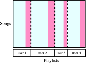
(a) Cold Playlists

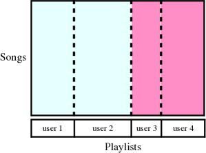
(b) Cold Users

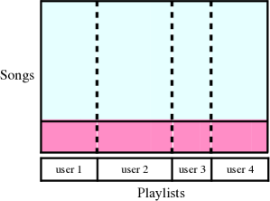
(c) Cold Songs

Figure 1: Three settings of cold-start playlist recommendation. In each setting, rows represent songs, and a column represents a playlist, which is a binary vector where an element denotes if the corresponding song is in the playlist. Playlists are grouped by user. Light Cyan represents playlists or songs in the training set, and dark Magenta represents playlists or songs in the test set. (a) Cold Playlists: recommending personalised playlists (Magenta) for each user given users’ existing playlists (Cyan); (b) Cold Users: recommending playlists for new users (Magenta) given playlists from existing users (Cyan); (c) Cold Songs: recommending newly released songs (Magenta) to extend users’ existing playlists (Cyan).

We first define the three cold-start settings considered in this paper, then introduce the multitask learning objective and show how the problem of cold-start playlist recommendation can be handled. We discuss the challenge in optimising the multitask learning objective via convex constrained optimisation and show how one can efficiently approximate an optimal solution by minimising an unconstrained objective.

Cold playlists, cold users and cold songs

Figure 1 illustrates the three cold-start settings for playlist recommendation that we study in this paper:

1. Cold playlists, where we recommend songs to form new personalised playlists for each existing user;

2. Cold users, where we recommend songs to form new playlists for each new user;

3. Cold songs, where we recommend newly released songs to extend users’ existing playlists.

In the cold playlists setting, a target user (i.e., the one for whom we recommend playlists) maintains a number of playlists that can be exploited by the learning algorithm. In the cold users setting, however, we may only know a few simple attributes of a new user (e.g., age, gender, country) or nothing except her user identifier. The learning algorithm can only make use of playlists from existing users. Finally, in the cold songs setting, the learning algorithm have access to content features (e.g., artist, genre, audio data) of newly released songs as well as all playlists from existing users.

Multitask learning objective

Suppose we have a dataset $\mathcal{D}$ with $N$ playlists from $U$ users, where songs in every playlist are from a music collection with $M$ songs. Assume each user has at least one playlist, and each song in the collection appears in at least one playlist. Let $P_{u}$ denote the (indices of) playlists from user $u\in\{1,\dots,U\}$. We aim to learn a function $f(m,u,i)$ that measures the affinity between song $m\in\{1,\dots,M\}$ and playlist $i\in P_{u}$ from user $u$. Suppose for song $m$, function $f$ has linear form,

$$f(m,u,i)=\mathbf{w}_{u,i}^{\top}\mathbf{x}_{m},$$ (1)

where $\mathbf{x}_{m}\in\mathbb{R}^{D}$ represents the $D$ features of song $m$, and $\mathbf{w}_{u,i}\in\mathbb{R}^{D}$ are the weights of playlist $i$ from user $u$.

Inspired by the decomposition of user weights and artist weights in (?), we decompose $\mathbf{w}_{u,i}$ into three components

$$\mathbf{w}_{u,i}={\bm{\alpha}}_{u}+{\bm{\beta}}_{i}+\bm{\mu},$$ (2)

where ${\bm{\alpha}}_{u}$ are weights for user $u$, ${\bm{\beta}}_{i}$ are weights specific for playlist $i$, and $\bm{\mu}$ are the weights shared by all users (and playlists). This decomposition allows us to learn the user weights ${\bm{\alpha}}_{u}$ using all her playlists, and exploit all training playlists when learning the shared weights $\bm{\mu}$.

Let ${\bm{\uptheta}}$ denote all parameters in $\left\{\{{\bm{\alpha}}_{u}\}_{u=1}^{U},\{{\bm{\beta}}_{i}\}_{i=1}^{N},\bm{\mu}\right\}$. The learning task is to minimise the empirical risk of affinity function $f$ on dataset $\mathcal{D}$ over ${\bm{\uptheta}}$, i.e.,

$$\min_{\bm{\uptheta}}\,\Omega({\bm{\uptheta}})+R_{\bm{\uptheta}}(f,\mathcal{D}),$$ (3)

where $\Omega({\bm{\uptheta}})$ is a regularisation term and $R_{\bm{\uptheta}}(f,\mathcal{D})$ denotes the empirical risk of $f$ on $\mathcal{D}$. We call the objective in problem (3) the multitask learning objective, since we jointly learn from multiple tasks where each one involves recommending a set of songs given a user or playlist.

We further assume that playlists from the same user have similar weights and the shared weights $\bm{\mu}$ are sparse (i.e., users only share a small portion of their weights). To impose these assumptions, we apply $\ell_{1}$ regularisation to encourage sparsity of the playlist weights ${\bm{\beta}}_{i}$ and the shared weights $\bm{\mu}$. The regularisation term in our multitask learning objective is

$$\Omega({\bm{\uptheta}})=\lambda_{1}\sum_{u=1}^{U}\|{\bm{\alpha}}_{u}\|_{2}^{2}+\lambda_{2}\sum_{i=1}^{N}\|{\bm{\beta}}_{i}\|_{1}+\lambda_{3}\|\bm{\mu}\|_{1},$$

where constants $\lambda_{1},\lambda_{2},\lambda_{3}\in\mathbb{R}_{+}$, and the $\ell_{2}$ regularisation term is to penalise large values in user weights. We specify the empirical risk $R_{\uptheta}(f,\mathcal{D})$ later.

Cold-start playlist recommendation

Once parameters $\uptheta$ have been learned, we make a recommendation by first scoring each song according to available information (e.g., an existing user or playlist), then form or extend a playlist by either taking the top-$K$ scored songs or sampling songs with probabilities proportional to their scores. Specifically, in the cold playlists setting where the target user $u$ is known, we score song $m$ as

$$r_{m}^{(a)}=({\bm{\alpha}}_{u}+\bm{\mu})^{\top}\mathbf{x}_{m}.$$ (4)

Further, in the cold users setting where simple attributes of the new user are available, we approximate the weights of the new user using the average weights of similar existing users (e.g., in terms of cosine similarity of user attributes) and score song $m$ as

$$r_{m}^{(b)}=\left(\frac{1}{|\mathcal{U}|}\sum_{u\in\mathcal{U}}{\bm{\alpha}}_{u}+\bm{\mu}\right)^{\top}\mathbf{x}_{m},$$ (5)

where $\mathcal{U}$ is the set of (e.g., 10) existing users that are most similar to the new user. On the other hand, if we know nothing about the new user except her identifier, we can simply score song $m$ using the shared weights, i.e.,

$$r_{m}^{(b)}=\bm{\mu}^{\top}\mathbf{x}_{m}.$$ (6)

Lastly, in the cold songs setting where we are given a specific playlist $i$ from user $u$, we therefore can score song $m$ using both user weights and playlist weights, i.e.,

$$r_{m}^{(c)}=({\bm{\alpha}}_{u}+{\bm{\beta}}_{i}+\bm{\mu})^{\top}\mathbf{x}_{m}.$$ (7)

We now specify the empirical risk $R_{\uptheta}(f,D)$ and develop methods to optimise the multitask learning objective.

Constrained optimisation with ranking loss

We aim to rank songs that are likely in a playlist above those that are unlikely when making a recommendation. To achieve this, we optimise the multitask learning objective by minimising a bipartite ranking loss. In particular, we minimise the number of songs not in a training playlist but ranked above the lowest ranked song in it. The loss of the affinity function $f$ for playlist $i$ from user $u$ is defined as

where $M_{-}^{i}$ is the number of songs not in playlist $i$, binary variable $y_{m}^{i}$ denotes whether song $m$ appears in playlist $i$, and $\llbracket\cdot\rrbracket$ is the indicator function that represents the 0/1 loss.

The empirical risk when employing the bipartite ranking loss $\Delta_{f}(u,i)$ is

$$R_{{\bm{\uptheta}}}^{\textsc{rank}}(f,\mathcal{D})=\frac{1}{N}\sum_{u=1}^{U}\sum_{i\in P_{u}}\Delta_{f}(u,i).$$ (8)

There are two challenges when optimising the multitask learning objective in problem (3) with the empirical risk $R_{\uptheta}^{\textsc{rank}}$, namely, the non-differentiable 0/1 loss and the min function in $\Delta_{f}(u,i)$. To address these challenges, we first upper-bound the 0/1 loss with one of its convex surrogates, e.g., the exponential loss $\llbracket z\leq 0\rrbracket\leq e^{-z}$,

One approach to deal with the min function in $\Delta_{f}(u,i)$ is introducing slack variables $\xi_{i}$ to lower-bound the scores of songs in playlist $i$ and transform problem (3) with empirical risk $R_{\uptheta}^{\textsc{rank}}$ into a convex constrained optimisation problem

Note that the number of constraints in the above optimisation problem is $\sum_{u=1}^{U}\sum_{i\in P_{u}}\sum_{m=1}^{M}\,\llbracket y_{m}^{i}\!=\!1\rrbracket,$ i.e., the accumulated playcount of all songs, which is of order $O(\mkern 1.5mu\overline{\mkern-2.5muL\mkern-1.5mu}\mkern 1.5muN)$ asymptotically, where $\mkern 1.5mu\overline{\mkern-2.5muL\mkern-1.5mu}\mkern 1.5mu$ is the average number of songs in playlists (typically less than $100$). However, the total number of playlists $N$ can be enormous in production systems (e.g., Spotify hosts more than $2$ billion playlists), which imposes a significant challenge in optimisation. This issue could be alleviated by applying the cutting-plane method (?) or the sub-gradient method. Unfortunately, we find both methods converge extremely slowly for this problem in practice. In particular, the cutting plane method is required to solve a constrained optimisation problem with at least $N$ constraints in each iteration, which remains challenging.

Unconstrained optimisation with classification loss

An alternative approach to deal with the min function in $\Delta_{f}(u,i)$ is approximating it using the well known Log-sum-exp function (?, p. 72),

$$\min_{j}z_{j}=\displaystyle-\max_{j}(-z_{j})=\displaystyle-\lim_{p\to+\infty}\frac{1}{p}\log\sum_{j}\exp(-pz_{j}),$$

which allows us to approximate the empirical risk $R_{{\bm{\uptheta}}}^{\textsc{rank}}$ (with the exponential surrogate) by $\widetilde{R}_{{\bm{\uptheta}}}^{\textsc{rank}}$ defined as

where hyper-parameter $p\in\mathbb{R}_{+}$ and

$$\delta_{f}(m,u,i)=\!\!\sum_{m^{\prime}:y_{m^{\prime}}^{i}=0}\!\!\exp(-(f(m,u,i)-f(m^{\prime},u,i))).$$

We further observe that $\widetilde{R}_{{\bm{\uptheta}}}^{\textsc{rank}}$ can be transformed into the standard P-Norm Push loss (?) by simply swapping the positives $\{m:y_{m}^{i}=1\}$ and negatives $\{m^{\prime}:y_{m^{\prime}}^{i}=0\}$. Inspired by the connections between bipartite ranking and binary classification (?), we swap the positives and negatives in the P-Classification loss (?) while taking care of signs. This results in an empirical risk with a classification loss:

where $M_{+}^{i}$ is the number of songs in playlist $i$.

Lemma 1.

Let ${\bm{\uptheta}}^{*}\in\operatorname*{argmin}_{{\bm{\uptheta}}}R_{{\bm{\uptheta}}}^{\textsc{mtc}}$ (assuming minimisers exist), then ${\bm{\uptheta}}^{*}\in\operatorname*{argmin}_{{\bm{\uptheta}}}\widetilde{R}_{{\bm{\uptheta}}}^{\textsc{rank}}$.

Proof.

See Appendix for a complete proof. Alternatively, we can use the proof of the equivalence between P-Norm Push loss and P-Classification loss (?) if we swap the positives and negatives. ∎

By Lemma 1, we can optimise the parameters of the multitask learning objective by solving a (convex) unconstrained optimisation problem:

$$\min_{\bm{\uptheta}}\ \Omega({\bm{\uptheta}})+R_{{\bm{\uptheta}}}^{\textsc{mtc}}(f,\mathcal{D}).$$ (10)

Problem (10) can be efficiently optimised using the Orthant-Wise Limited-memory Quasi-Newton (OWL-QN) algorithm (?), an L-BFGS variant that can address $\ell_{1}$ regularisation effectively.

We refer to the approach that solves problem (10) as Multitask Classification (MTC). As a remark, optimal solutions of problem (10) are not necessarily the optimal solutions of problem $\min_{\bm{\uptheta}}\ \Omega({\bm{\uptheta}})+\widetilde{R}_{{\bm{\uptheta}}}^{\textsc{rank}}$ due to regularisation. However, when parameters ${\bm{\uptheta}}$ are small (which is generally the case when using regularisation), optimal solutions of the two objectives can nonetheless approximate each other well.

Related work

We summarise recent work most related to playlist recommendation and music recommendation in cold-start scenarios, as well as work on the connection between bipartite ranking and binary classification.

There is a rich collection of recent literature on playlist recommendation, which can be summarised into two typical settings: playlist generation and next song recommendation. Playlist generation is to produce a complete playlist given some seed. For example, the AutoDJ system (?) generates playlists given one or more seed songs; Groove Radio can produce a personalised playlist for the specified user given a seed artist (?); or a seed location in hidden space (where all songs are embedded) can be specified in order to generate a complete playlist (?). There are also works that focus on evaluating the learned playlist model, without concretely generating playlists (?; ?). See this recent survey (?) for more details.

Next song recommendation predicts the next song a user might play after observing some context. For example, the most recent sequence of songs with which a user has interacted was used to infer the contextual information, which was then employed to rank the next possible song via a topic-based sequential model learned from users’ playlists (?). Context can also be the artists in a user’s listening history, which has been employed to score the next song together with frequency of artist collocations as well as song popularity (?; ?). It is straightforward to produce a complete playlist using next song recommendation techniques, i.e., by picking the next song sequentially (?; ?).

In the collaborative filtering literature, the cold-start setting has primarily been addressed through suitable regularisation of matrix factorisation parameters based on exogenous user- or item-features (?; ?; ?). Content-based approaches (?, chap. 4) can handle the recommendation of new songs, typically by making use of content features of songs extracted either automatically (?; ?) or manually by musical experts (?). Further, content features can also be combined with other approaches, such as those based on collaborative filtering (?; ?; ?), which is known as the hybrid recommendation approach (?; ?).

Another popular approach for cold-start recommendation involves explicitly mapping user- or item- content features to latent embeddings (?). This approach can be adopted to recommend new songs, e.g., by learning a convolutional neural network to map audio features of new songs to the corresponding latent embeddings (?), which were then used to score songs together with the latent embeddings of playlists (learned by MF). The problem of recommending music for new users can also be tackled using a similar approach, e.g., by learning a mapping from user attributes to user embeddings.

A slightly different approach to deal with music recommendation for new users is learning hierarchical representations for genre, sub-genre and artist. By adopting an additive form with user and artist weights, it can fall back to using only artist weights when recommending music to new users; if the artist weights are not available (e.g., a new artist), this approach further falls back to using the weights of sub-genre or genre (?). However, the requirement of seed information (e.g., artist, genre or a seed song) restricts its direct applicability to the cold playlists and cold users settings. Further, encoding song usage information as features makes it unsuitable for recommending new songs directly.

It is well known that bipartite ranking and binary classification are closely related (?; ?). In particular, ? (?) have shown that the P-Norm Push (?) is equivalent to the P-Classification when the exponential surrogate of 0/1 loss is employed. Further, the P-Norm Push is an approximation of the Infinite-Push (?), or equivalently, the Top-Push (?), which focuses on the highest ranked negative example instead of the lowest ranked positive example in the Bottom-Push adopted in this work. Compared to the Bayesian Personalised Ranking (BPR) approach (?; ?) that requires all positive items to be ranked higher than those unobserved ones, the adopted approach only penalises unobserved items that ranked higher than the lowest ranked positive item, which can be optimised more efficiently when only the top ranked items are of interest (?; ?).

Experiments

We present empirical evaluations for cold-start playlist recommendation on two real playlist datasets, and compare the proposed multitask learning method with a number of well known baseline approaches.

Dataset

We evaluate on two publicly available playlist datasets: the 30Music (?) and the AotM-2011 (?) dataset. The Million Song Dataset (MSD) (?) serves as an underlying dataset where songs in all playlists are intersected; additionally, song and artist information in the MSD are used to compute song features.

30Music Dataset is a collection of listening events and user-generated playlists retrieved from Last.fm. We first intersect the playlists data with songs in the MSD, then filter out playlists with less than 5 songs. This results in about 17K playlists over 45K songs from 8K users.

AotM-2011 Dataset is a collection of playlists shared by Art of the Mix users during the period from 1998 to 2011. Songs in playlists have been matched to those in the MSD. It contains roughly 84K playlists over 114K songs from 14K users after filtering out playlists with less than 5 songs.

Table 1 summarises the two playlist datasets used in this work. See Appendix for more details.

Features

Song metadata, audio data, genre and artist information, as well as song popularity (i.e., the accumulated playcount of the song in the training set) and artist popularity (i.e., the accumulated playcount of all songs from the artist in the training set) are encoded as features. The metadata of songs (e.g., duration, year of release) and pre-computed audio features (e.g., loudness, mode, tempo) are from the MSD. We use genre data from the Top-MAGD genre dataset (?) and tagtraum genre annotations for the MSD (?) via one-hot encoding. If the genre of a song is unknown, we apply mean imputation using genre counts of songs in the training set. To encode artist information as features, we create a sequence of artist identifiers for each playlist in the training set, and train a word2vec model that learns embeddings of artists. We assume no popularity information is available for newly released songs, and therefore song popularity is not a feature in the cold songs setting. Finally, we add a constant feature (with value $1.0$) for each song to account for bias.

Table 1: Statistics of music playlist datasets

	30Music	AotM-2011
Playlists	17,457	84,710
Users	8,070	14,182
Avg. Playlists per User	2.2	6.0
Songs	45,468	114,428
Avg. Songs per Playlist	16.3	10.1
Artists	9,981	15,698
Avg. Songs per Artist	28.6	53.8

Experimental setup

We first split the two playlist datasets into training and test sets, then evaluate the test set performance of the proposed method, and compare it against several baseline approaches in each of the three cold-start settings.

Dataset split

In the cold playlists setting, we hold a portion of the playlists from about 20% of users in both datasets for testing, and all other playlists are used for training. The test set is formed by sampling playlists where each song has been included in at least five playlists among the whole dataset. We also make sure each song in the test set appears in the training set, and all users in the test set have a few playlists in the training set. In the cold users setting, we sample 30% of users and hold all of their playlists in both datasets. Similarly, we require songs in the test set to appear in the training set, and a user will thus not be used for testing if holding all of her playlists breaks this requirement. To evaluate in the cold songs setting, we hold 5K of the latest released songs in the 30Music dataset, and 10K of the latest released songs in the AotM-2011 dataset where more songs are available. We remove playlists where all songs have been held for testing.

See Appendix for the statistics of these dataset splits.

Table 2: AUC for playlist recommendation in three cold-start settings. Higher values indicate better performance.

Cold Playlists					Cold Users					Cold Songs
Method	30Music	AotM-2011			Method	30Music	AotM-2011			Method	30Music	AotM-2011
PopRank	94.0	93.8			PopRank	88.3	91.8			PopRank	70.9	76.5
CAGH	94.8	94.2			CAGH	86.3	88.1			CAGH	68.0	77.4
SAGH	64.5	79.8			SAGH	54.5	53.7			SAGH	51.5	53.6
WMF	79.5	85.4			WMF+kNN	84.9	N/A			MF+MLP	81.4	80.8
MTC	95.9	95.4			MTC	88.8	91.8			MTC	86.6	84.3

Baselines

We compare the performance of our proposed method (i.e., MTC) with the following baseline approaches in each of the three cold-start settings:

• The Popularity Ranking (PopRank) method scores a song using only its popularity in the training set. In the cold songs setting where song popularity is not available, a song is scored by the popularity of the corresponding artist.

• The Same Artists - Greatest Hits (SAGH) (?) method scores a song by its popularity if the artist of the song appears in the given user’s playlists (in the training set); otherwise the song is scored zero. In the cold songs setting, this method only considers songs from artists that appear in the given playlist, and scores a song using the popularity of the corresponding artist.

• The Collocated Artists - Greatest Hits (CAGH) (?) method is a variant of SAGH. It scores a song using its popularity, but weighted by the frequency of the collocation between the artist of the song and artists that appear in the given user’s playlists (in the training set). In the cold users setting, we use the 10 most popular artists instead of artists in the user’s listening history, and the cold songs setting is addressed in the same way as in SAGH.

• A variant of Matrix Factorisation (MF), which first learns the latent factors of songs, playlists or users through MF, then scores each song by the dot product of the corresponding latent factors. Recommendations are made as per the proposed method. In the cold playlists setting, we factorise the song-user playcount matrix using the weighted matrix factorisation (WMF) algorithm (?), which learns the latent factors of songs and users. In the cold users setting, we first learn the latent factors of songs and users using WMF, then approximate the latent factors of a new user by the average latent factors of the $k$ (e.g., 100) nearest neighbours (in terms of cosine similarity of user attributes, e.g., age, gender and country) in the training set. We call this method WMF+kNN. In the cold songs setting, we factorise the song-playlist matrix to learn the latent factors of songs and playlists, which are then used to train a neural network to map song content features to the corresponding latent factors (?; ?). We can then obtain the latent factors of a new song as long as its content features are available. We call this method MF+MLP.

Evaluation

We evaluate all approaches using two accuracy metrics that have been adopted in playlist recommendation tasks: HitRate@K (?) and Area under the ROC curve (AUC) (?). We further adopt two beyond-accuracy metrics: Novelty (?; ?) and Spread (?), which are specifically tailored to recommender systems.

HitRate@K (i.e., Recall@K) is the number of correctly recommended songs amongst the top-$K$ recommendations over the number of songs in the observed playlist. It has been widely employed to evaluate playlist generation and next song recommendation methods (?; ?; ?; ?). AUC has been primarily used to measure the performance of classifiers. It has been applied to evaluate playlist generation methods when the task has been cast as a sequence of classification problems (?).

It is believed that useful recommendations need to include previously unknown items (?; ?). This ability can be measured by Novelty, which is based on the assumption that, intuitively, the more popular a song is, the more likely a user is to be familiar with it, and therefore the less likely to be novel. Spread, however, is used to measure the ability of an algorithm to spread its attention across all possible songs. It is defined as the entropy of the distribution of all songs. See Appendix for more details of these beyond-accuracy metrics.

Results and discussion

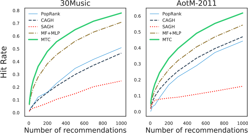
Figure 2: Hit rate of recommendation in the cold songs setting. Higher values indicate better performance.

Table 3: Spread for playlist recommendation in three cold-start settings. Moderate values are preferable.

Cold Playlists					Cold Users					Cold Songs
Method	30Music	AotM-2011			Method	30Music	AotM-2011			Method	30Music	AotM-2011
PopRank	9.8	10.5			PopRank	9.8	10.5			PopRank	7.4	7.8
CAGH	5.8	2.3			CAGH	4.2	5.3			CAGH	4.3	4.6
SAGH	10.3	10.4			SAGH	10.0	10.7			SAGH	6.5	5.9
WMF	10.7	11.6			WMF+kNN	10.7	N/A			MF+MLP	8.5	9.2
MTC	9.4	10.4			MTC	9.9	11.4			MTC	7.9	8.3

Accuracy

Table 2 shows the performance of all methods in terms of AUC. We can see that PopRank achieves good performance in all three cold-start settings. This is in line with results reported in (?; ?). Artist information, particularly the frequency of artist collocations that is exploited in CAGH, improves recommendation in the cold playlists and cold songs settings. Further, PopRank is one of the best performing methods in the cold users setting, which is consistent with previous discoveries (?; ?; ?). The reason is believed to be the long-tailed distribution of songs in playlists (?; ?). The MF variant does not perform well in the cold playlists setting, but it performs reasonably well in the cold users setting when attributes of new users are available (e.g., in the 30Music dataset), and it works particularly well in the cold songs setting where both song metadata and audio features are available for new songs.

Lastly, MTC is the (tied) best performing method in all three cold-start settings on both datasets. Interestingly, it achieves the same performance as PopRank in the cold users setting on the AotM-2011 dataset, which suggests that MTC might degenerate to simply ranking songs according to popularity when making recommendations for new users; however, when attributes of new users are available, it can improve by exploiting information learned from existing users.

Figure 2 shows the hit rate of all methods in the cold songs setting when the number of recommended new songs varies from 5 to 1000. As expected, the performance of all methods improves when the number of recommendations increases. Further, we observe that learning based approaches (i.e., MTC and MF+MLP) always perform better than other baselines that use only artist information. works surprisingly well; it even outperforms CAGH which exploits artist collocations on the 30Music dataset. The fact that CAGH always performs better than SAGH confirms that artist collocation is helpful for music recommendation. Lastly, MTC outperforms all other methods by a big margin on both datasets, which demonstrates the effectiveness of the proposed approach for recommending new songs.

We also observe that MTC improves over baselines in the cold playlists and cold users settings (when simple attributes of new users are available), although the margin is not as big as that in the cold songs setting. See Appendix for details.

Beyond accuracy

Note that, unlike AUC and hit rate, where higher values indicate better performance, moderate values of Spread and Novelty are usually preferable (?; ?).

Table 3 shows the performance of all recommendation approaches in terms of Spread. In the cold songs setting, CAGH and SAGH focus on songs from artists in users’ listening history and similar artists, which explains the relative low Spread. However, in the cold playlists and cold users settings, SAGH improves its attention spreading due to the set of songs it focuses on is significantly bigger (i.e., songs from all artists in users’ previous playlists and songs from the 10 most popular artists, respectively). Surprisingly, CAGH remains focusing on a relatively small set of songs in both settings. Lastly, in all three cold-start settings, the MF variants have the highest Spread, while both PopRank and MTC have (similar) moderate Spread, which is considered better.

Figure 3 shows the Novelty of all methods in the cold playlists setting. We can see that PopRank has the lowest Novelty, which is not surprising given the definition of Novelty (see Appendix). Both SAGH and CAGH start with low Novelty and grow when the number of recommended songs increases, but the Novelty of CAGH saturates much earlier than that of SAGH. The reason could be that, when the number of recommendations is larger than the total number of songs from artists in a user’s previous playlists, SAGH will simply recommend songs randomly (which are likely to be novel) while CAGH will recommend songs from artists that are similar to those in the user’s previous playlists (which could be comparably less novel). Further, MTC achieves lower Novelty than WMF and CAGH, which indicates that MTC tends to recommend popular songs to form new playlists. To conclude, MTC and CAGH have moderate Novelty on both datasets, and therefore perform better than other approaches.

The proposed approach also achieves moderate Novelty in the cold songs setting. However, in the cold users setting, the MF variant and CAGH have moderate Novelty, which are therefore preferred. See Appendix for details.

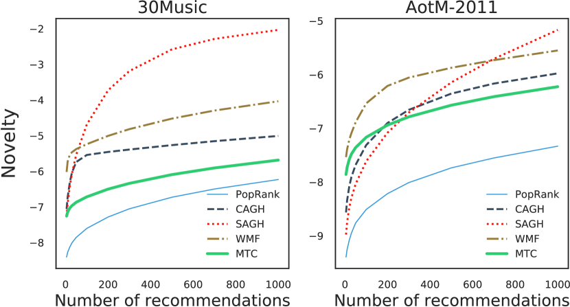
Figure 3: Novelty of recommendation in the cold playlists setting. Moderate values are preferable.

Conclusion and future work

We study the problem of recommending playlists to users in three cold-start settings: cold playlists, cold users and cold songs. We propose a multitask learning method that learns user- and playlist-specific weights as well as shared weights from user-curated playlists, which allows us to form new personalised playlists for an existing user, produce playlists for a new user, and extend users’ playlists with newly released songs. We optimise the parameters (i.e., weights) by minimising a bipartite ranking loss that encourages songs in a playlist to be ranked higher than those that are not. An equivalence between bipartite ranking and binary classification further enables efficient approximation of optimal parameters. Empirical evaluations on two real playlist datasets demonstrate the effectiveness of the proposed method for cold-start playlist recommendation. For future work, we would like to explore auxiliary data sources (e.g., music information shared on social media) and additional features of songs and users (e.g., lyrics, user profiles) to make better recommendations. Further, non-linear models such as deep neural networks have been shown to work extremely well in a wide range of tasks, and the proposed linear model with sparse parameters could be more compact if a non-linear model were adopted.

Appendix to “Cold-start Playlist Recommendation with Multitask Learning”

Appendix A Proof of Lemma 1

First, we can approximate the empirical risk $R_{\uptheta}^{\textsc{rank}}$ (with the exponential surrogate) as follows:

$$R_{\uptheta}^{\textsc{rank}}(f,\mathcal{D}) =\frac{1}{N}\sum_{u=1}^{U}\sum_{i\in P_{u}}\frac{1}{M_{-}^{i}}\sum_{m^{\prime}:y_{m^{\prime}}^{i}=0}\exp\left(-\min_{m:y_{m}^{i}=1}f(m,u,i)+f(m^{\prime},u,i)\right)$$

$$=\frac{1}{N}\sum_{u=1}^{U}\sum_{i\in P_{u}}\frac{1}{M_{-}^{i}}\exp\left(-\min_{m:y_{m}^{i}=1}f(m,u,i)\right)\sum_{m^{\prime}:y_{m^{\prime}}^{i}=0}\exp\left(f(m^{\prime},u,i)\right)$$

$$\approx\frac{1}{N}\sum_{u=1}^{U}\sum_{i\in P_{u}}\frac{1}{M_{-}^{i}}\exp\left(\frac{1}{p}\log\sum_{m:y_{m}^{i}=1}e^{-pf(m,u,i)}\right)\sum_{m^{\prime}:y_{m^{\prime}}^{i}=0}\exp\left(f(m^{\prime},u,i)\right)$$

$$=\frac{1}{N}\sum_{u=1}^{U}\sum_{i\in P_{u}}\frac{1}{M_{-}^{i}}\left(\sum_{m:y_{m}^{i}=1}e^{-pf(m,u,i)}\right)^{\frac{1}{p}}\sum_{m^{\prime}:y_{m^{\prime}}^{i}=0}e^{f(m^{\prime},u,i)}$$

$$=\frac{1}{N}\sum_{u=1}^{U}\sum_{i\in P_{u}}\frac{1}{M_{-}^{i}}\left(\left(\sum_{m^{\prime}:y_{m^{\prime}}^{i}=0}e^{f(m^{\prime},u,i)}\right)^{p}\sum_{m:y_{m}^{i}=1}e^{-pf(m,u,i)}\right)^{\frac{1}{p}}$$

$$=\frac{1}{N}\sum_{u=1}^{U}\sum_{i\in P_{u}}\frac{1}{M_{-}^{i}}\left(\sum_{m:y_{m}^{i}=1}e^{-pf(m,u,i)}\left(\sum_{m^{\prime}:y_{m^{\prime}}^{i}=0}e^{f(m^{\prime},u,i)}\right)^{p}\right)^{\frac{1}{p}}$$

$$=\frac{1}{N}\sum_{u=1}^{U}\sum_{i\in P_{u}}\frac{1}{M_{-}^{i}}\left(\sum_{m:y_{m}^{i}=1}\left(\sum_{m^{\prime}:y_{m^{\prime}}^{i}=0}e^{-\left(f(m,u,i)-f(m^{\prime},u,i)\right)}\right)^{p}\right)^{\frac{1}{p}}$$

$$=\widetilde{R}_{\uptheta}^{\textsc{rank}}(f,\mathcal{D}).$$

Recall that $R_{\uptheta}^{\textsc{mtc}}$ is the following classification risk:

$$R_{\uptheta}^{\textsc{mtc}}(f,\mathcal{D})=\frac{1}{N}\sum_{u=1}^{U}\sum_{i\in P_{u}}\left(\frac{1}{pM_{+}^{i}}\sum_{m:y_{m}^{i}=1}e^{-pf(m,u,i)}+\frac{1}{M_{-}^{i}}\sum_{m^{\prime}:y_{m^{\prime}}^{i}=0}e^{f(m^{\prime},u,i)}\right),$$

Let $\uptheta^{*}\in\operatorname*{argmin}_{\uptheta}R_{\uptheta}^{\textsc{mtc}}$ (assuming minimisers exist), we want to prove that $\uptheta^{*}\in\operatorname*{argmin}_{\uptheta}\widetilde{R}_{\uptheta}^{\textsc{rank}}$.

Proof.

We follow the proof technique in (?) by first introducing a constant feature $1$ for each song, without loss of generality, let the first feature of $\mathbf{x}_{m},\,m\in\{1,\dots,M\}$ be the constant feature, i.e., $x_{m}^{0}=1$. We can show that $\frac{\partial\,R_{\uptheta}^{\textsc{mtc}}}{\partial\,\uptheta}=0$ implies $\frac{\partial\,\widetilde{R}_{\uptheta}^{\textsc{rank}}}{\partial\,\uptheta}=0$, which means minimisers of $R_{\uptheta}^{\textsc{mtc}}$ also minimise $\widetilde{R}_{\uptheta}^{\textsc{rank}}$.

Let $\displaystyle 0=\frac{\partial\,R_{\uptheta}^{\textsc{mtc}}}{\partial\,\beta_{i}^{0}}=\frac{1}{N}\left(\frac{1}{pM_{+}^{i}}\sum_{m:y_{m}^{i}=1}e^{-pf(m,u,i)}(-p)+\frac{1}{M_{-}^{i}}\sum_{m^{\prime}:y_{m^{\prime}}^{i}=0}e^{f(m^{\prime},u,i)}\right),\ \forall i\in P_{u},\,u\in\{1,\dots,U\},$

we have

$$\frac{1}{M_{+}^{i}}\sum_{m:y_{m}^{i}=1}e^{-pf(m,u,i)}\Bigg{|}_{\uptheta=\uptheta^{*}}=\frac{1}{M_{-}^{i}}\sum_{m^{\prime}:y_{m^{\prime}}^{i}=0}e^{f(m^{\prime},u,i)}\Bigg{|}_{\uptheta=\uptheta^{*}},\ \forall i\in P_{u},\,u\in\{1,\dots,U\},$$ (11)

Further, let

$$\mathbf{0}=\frac{\partial\,R_{\uptheta}^{\textsc{mtc}}}{\partial\,{\bm{\beta}}_{i}}=\frac{1}{N}\left(\frac{1}{pM_{+}^{i}}\sum_{m:y_{m}^{i}=1}e^{-pf(m,u,i)}(-p\mathbf{x}_{m})+\frac{1}{M_{-}^{i}}\sum_{m^{\prime}:y_{m^{\prime}}^{i}=0}e^{f(m^{\prime},u,i)}\mathbf{x}_{m^{\prime}}\right),\ \forall i\in P_{u},\,u\in\{1,\dots,U\},$$

we have

$$\frac{1}{M_{+}^{i}}\sum_{m:y_{m}^{i}=1}e^{-pf(m,u,i)}\mathbf{x}_{m}\Bigg{|}_{\uptheta=\uptheta^{*}}=\frac{1}{M_{-}^{i}}\sum_{m^{\prime}:y_{m^{\prime}}^{i}=0}e^{f(m^{\prime},u,i)}\mathbf{x}_{m^{\prime}}\Bigg{|}_{\uptheta=\uptheta^{*}},\ \forall i\in P_{u},\,u\in\{1,\dots,U\}.$$ (12)

Note that $\forall i\in P_{u},\,u\in\{1,\dots,U\}$,

Let

$$h(u,i)=\frac{1}{NM_{-}^{i}}\left(\sum_{m:y_{m}^{i}=1}e^{-pf(m,u,i)}\right)^{\frac{1}{p}}\sum_{m^{\prime}:y_{m^{\prime}}^{i}=0}e^{f(m^{\prime},u,i)},\ \forall i\in P_{u},\,u\in\{1,\dots,U\}.$$

Similar to Eq. (13), we have

$$\frac{\partial\,h(u,i)}{\partial\,{\bm{\beta}}_{i}}\Bigg{|}_{\uptheta=\uptheta^{*}}=\mathbf{0},\ \forall i\in P_{u},\,u\in\{1,\dots,U\}.$$ (14)

Note that $\forall u\in\{1,\dots,U\}$, by Eq. (14)

$$\frac{\partial\,\widetilde{R}_{\uptheta}^{\textsc{rank}}}{\partial\,{\bm{\alpha}}_{u}}\Bigg{|}_{\uptheta=\uptheta^{*}}=\sum_{i\in P_{u}}\frac{\partial\,h(u,i)}{\partial\,{\bm{\alpha}}_{u}}\Bigg{|}_{\uptheta=\uptheta^{*}}=\sum_{i\in P_{u}}\frac{\partial\,h(u,i)}{\partial\,{\bm{\beta}}_{i}}\Bigg{|}_{\uptheta=\uptheta^{*}}=\mathbf{0},$$ (15)

and

$$\frac{\partial\,\widetilde{R}_{\uptheta}^{\textsc{rank}}}{\partial\,\bm{\mu}}\Bigg{|}_{\uptheta=\uptheta^{*}}=\sum_{u=1}^{U}\sum_{i\in P_{u}}\frac{\partial\,h(u,i)}{\partial\,\bm{\mu}}\Bigg{|}_{\uptheta=\uptheta^{*}}=\sum_{u=1}^{U}\sum_{i\in P_{u}}\frac{\partial\,h(u,i)}{\partial\,{\bm{\beta}}_{i}}\Bigg{|}_{\uptheta=\uptheta^{*}}=\mathbf{0}.$$ (16)

Finally, by Eq. (13), Eq. (15), and Eq. (16), $\uptheta^{*}\in\operatorname*{argmin}_{\uptheta}\widetilde{R}_{\uptheta}^{\textsc{rank}}$.

∎

Appendix B Evaluation metrics

The four evaluation metrics used in this work are:

• HitRate@K, which is also known as Recall@K, is the number of correctly recommended songs amongst the top-$K$ recommendations over the number of songs in the observed playlist.

• Area under the ROC curve (AUC), which is the probability that a positive instance is ranked higher than a negative instance (on average).

• Novelty measures the ability of a recommender system to suggest previously unknown (i.e., novel) items,

  $$\text{Novelty@K}=\frac{1}{U}\sum_{u=1}^{U}\frac{1}{|P_{u}^{\textsc{test}}|}\sum_{i\in P_{u}^{\textsc{test}}}\sum_{m\in S_{K}^{i}}\frac{-\log_{2}pop_{m}}{K},$$

  where $P_{u}^{\textsc{test}}$ is the (indices of) test playlists from user $u$, $S_{K}^{i}$ is the set of top-$K$ recommendations for test playlist $i$ and $pop_{m}$ is the popularity of song $m$. Intuitively, the more popular a song is, the more likely a user is to be familiar with it, and therefore the less likely to be novel.

• Spread measures the ability of a recommender system to spread its attention across all possible items. It is defined as the entropy of the distribution of all songs,

  $$\text{Spread}=-\sum_{m=1}^{M}P(m)\log P(m),$$

  where $P(m)$ denotes the probability of song $m$ being recommended, which is computed from the scores of all possible songs using the softmax function in this work.

Appendix C Dataset

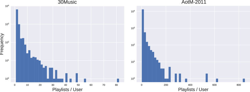
Figure 4: Histogram of the number of playlists per user

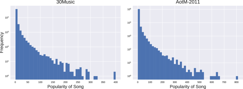
Figure 5: Histogram of song popularity

The histograms of the number of playlists per user as well as song popularity of the two datasets are shown in Figure 4 and Figure 5, respectively. We can see from Figure 4 and Figure 5 that both the number of playlists per user and song popularity follow a long-tailed distribution, which imposes further challenge to the learning task as the amount of data is very limited for users (or songs) at the tail.

The training and test split of the two playlist datasets in the three cold-start settings are shown in Table 4, Table 5, and Table 6, respectively.

Table 4: Dataset for cold playlists

Dataset	Training Set			Test Set
	Playlists	Users		Playlists	Users
30Music	15,262	8,070		2,195	1,644
AotM-2011	75,477	14,182		9,233	2,722

Table 5: Dataset for cold users

Dataset	Training Set			Test Set
	Users	Playlists		Users	Playlists
30Music	5,649	14,067		2,420	3,390
AotM-2011	9,928	76,450		4,254	8,260

Table 6: Dataset for cold songs

Dataset	Training Set			Test Set
	Songs	Playlists		Songs	Playlists
30Music	40,468	17,342		5,000	8,215
AotM-2011	104,428	84,646		10,000	19,504

Appendix D Empirical results

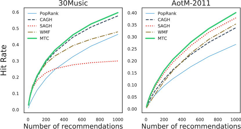
Figure 6: Hit rate of recommendation in the cold playlists setting. Higher values indicate better performance.

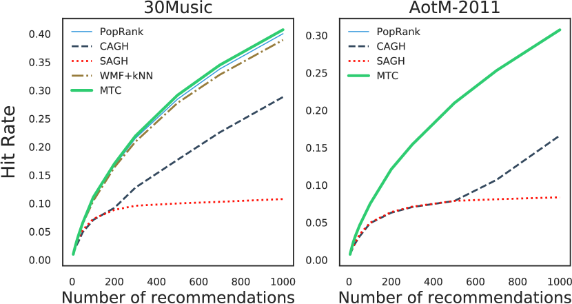
Figure 7: Hit rate of recommendation in the cold users setting. Higher values indicate better performance.

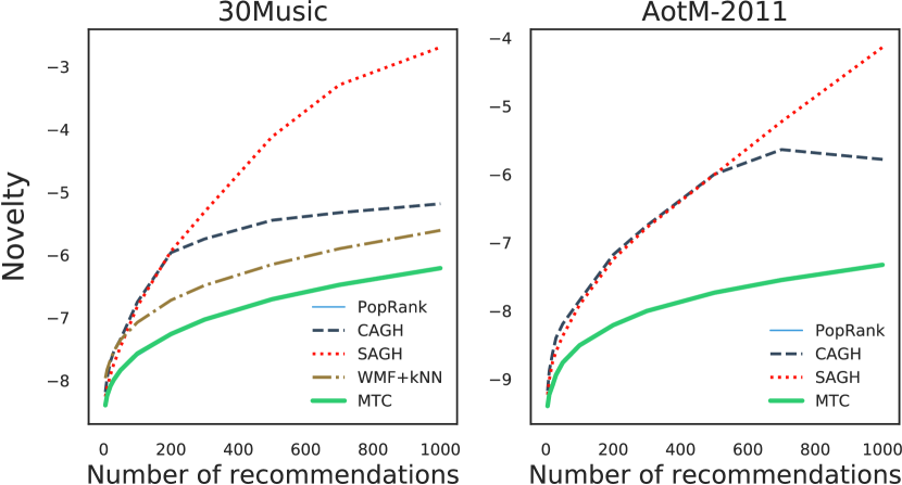
Figure 8: Novelty of recommendation in the cold users setting. Moderate values are preferable.

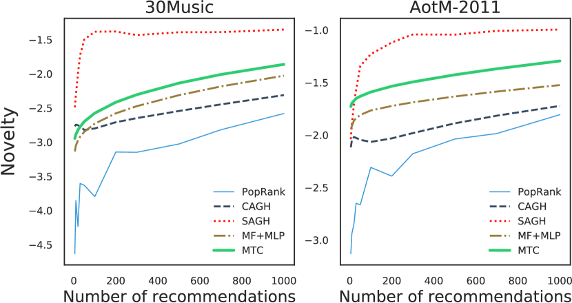
Figure 9: Novelty of recommendation in the cold songs setting. Moderate values are preferable.

Appendix E Notations

We introduce notations in Table 7.

Table 7: Notations used in this paper

Notation			Description
$D$	$\in$	$\mathbf{Z}^{+}\rule{10.0pt}{0.0pt}$	The number of features for each song
$M$	$\in$	$\mathbf{Z}^{+}$	The number of songs, indexed by $m,m^{\prime}\in\{1,\dots,M\}$
$M_{+}^{i}$	$\in$	$\mathbf{Z}^{+}$	The number of songs in playlist $i$
$M_{-}^{i}$	$\in$	$\mathbf{Z}^{+}$	The number of songs not in playlist $i$, i.e., $M_{-}^{i}=M-M_{+}^{i}$
$N$	$\in$	$\mathbf{Z}^{+}$	The total number of playlists from all users
$U$	$\in$	$\mathbf{Z}^{+}$	The number of users, indexed by $u\in\{1,\dots,U\}$
$P_{u}$			The set of indices of playlists from user $u$
${\bm{\alpha}}_{u}$	$\in$	$\mathbb{R}^{D}$	The weights of user $u$
${\bm{\beta}}_{i}$	$\in$	$\mathbb{R}^{D}$	The weights of playlist $i$ from user $u$, $i\in P_{u}$
$\bm{\mu}$	$\in$	$\mathbb{R}^{D}$	The weights shared by all users (and playlists)
$\mathbf{w}_{u,i}$	$\in$	$\mathbb{R}^{D}$	The weights of playlist $i$ from user $u$, $\mathbf{w}_{u,i}={\bm{\alpha}}_{u}+{\bm{\beta}}_{i}+\bm{\mu}$
$y_{m}^{i}$	$\in$	$\mathbb{R}^{D}$	The positive binary label $y_{m}^{i}=1$, i.e., song $m$ is in playlist $i$
$y_{m^{\prime}}^{i}$	$\in$	$\mathbb{R}^{D}$	The negative binary label $y_{m^{\prime}}^{i}=0$, i.e., song $m^{\prime}$ is not in playlist $i$
$\mathbf{x}_{m}$	$\in$	$\mathbb{R}^{D}$	The feature vector of song $m$

References

- [Agarwal and Chen, 2009] Agarwal, D. and Chen, B.-C. (2009). Regression-based latent factor models. In KDD.
- [Agarwal, 2011] Agarwal, S. (2011). The infinite push: A new support vector ranking algorithm that directly optimizes accuracy at the absolute top of the list. In ICDM.
- [Agarwal and Niyogi, 2005] Agarwal, S. and Niyogi, P. (2005). Stability and generalization of bipartite ranking algorithms. In COLT.
- [Aggarwal, 2016] Aggarwal, C. C. (2016). Recommender Systems: The Textbook. Springer.
- [Andrew and Gao, 2007] Andrew, G. and Gao, J. (2007). Scalable training of L1-regularized log-linear models. In ICML.
- [Avriel, 2003] Avriel, M. (2003). Nonlinear programming: analysis and methods. Courier Corporation.
- [Ben-Elazar et al., 2017] Ben-Elazar, S., Lavee, G., Koenigstein, N., Barkan, O., Berezin, H., Paquet, U., and Zaccai, T. (2017). Groove radio: A bayesian hierarchical model for personalized playlist generation. In WSDM.
- [Bertin-Mahieux et al., 2011] Bertin-Mahieux, T., Ellis, D. P., Whitman, B., and Lamere, P. (2011). The million song dataset. In ISMIR.
- [Bonnin and Jannach, 2013] Bonnin, G. and Jannach, D. (2013). Evaluating the quality of playlists based on hand-crafted samples. In ISMIR.
- [Bonnin and Jannach, 2015] Bonnin, G. and Jannach, D. (2015). Automated generation of music playlists: Survey and experiments. ACM Computing Surveys.
- [Boyd and Vandenberghe, 2004] Boyd, S. and Vandenberghe, L. (2004). Convex Optimization. Cambridge University Press.
- [Burke, 2002] Burke, R. (2002). Hybrid recommender systems: Survey and experiments. User modeling and user-adapted interaction, 12:331–370.
- [Cao et al., 2010] Cao, B., Liu, N. N., and Yang, Q. (2010). Transfer learning for collective link prediction in multiple heterogenous domains. In ICML.
- [Chen et al., 2012] Chen, S., Moore, J. L., Turnbull, D., and Joachims, T. (2012). Playlist prediction via metric embedding. In KDD.
- [Cremonesi et al., 2010] Cremonesi, P., Koren, Y., and Turrin, R. (2010). Performance of recommender algorithms on top-n recommendation tasks. In RecSys.
- [Donaldson, 2007] Donaldson, J. (2007). A hybrid social-acoustic recommendation system for popular music. In RecSys.
- [Eghbal-Zadeh et al., 2015] Eghbal-Zadeh, H., Lehner, B., Schedl, M., and Widmer, G. (2015). I-vectors for timbre-based music similarity and music artist classification. In ISMIR.
- [Ertekin and Rudin, 2011] Ertekin, Ş. and Rudin, C. (2011). On equivalence relationships between classification and ranking algorithms. JMLR, 12:2905–2929.
- [Freund et al., 2003] Freund, Y., Iyer, R., Schapire, R. E., and Singer, Y. (2003). An efficient boosting algorithm for combining preferences. JMLR, 4:933–969.
- [Gantner et al., 2010] Gantner, Z., Drumond, L., Freudenthaler, C., Rendle, S., and Schmidt-Thieme, L. (2010). Learning attribute-to-feature mappings for cold-start recommendations. In ICDM.
- [Hariri et al., 2012] Hariri, N., Mobasher, B., and Burke, R. (2012). Context-aware music recommendation based on latenttopic sequential patterns. In RecSys.
- [Herlocker et al., 2004] Herlocker, J. L., Konstan, J. A., Terveen, L. G., and Riedl, J. T. (2004). Evaluating collaborative filtering recommender systems. ACM Transactions on Information Systems, 22:5–53.
- [Hu et al., 2008] Hu, Y., Koren, Y., and Volinsky, C. (2008). Collaborative filtering for implicit feedback datasets. In ICDM.
- [Jannach et al., 2015] Jannach, D., Lerche, L., and Kamehkhosh, I. (2015). Beyond hitting the hits: Generating coherent music playlist continuations with the right tracks. In RecSys.
- [John, 2006] John, J. (2006). Pandora and the music genome project. Scientific Computing, 23:40–41.
- [Kluver and Konstan, 2014] Kluver, D. and Konstan, J. A. (2014). Evaluating recommender behavior for new users. In RecSys.
- [Koren et al., 2009] Koren, Y., Bell, R., and Volinsky, C. (2009). Matrix factorization techniques for recommender systems. Computer, 42:30–37.
- [Li et al., 2014] Li, N., Jin, R., and Zhou, Z.-H. (2014). Top rank optimization in linear time. In NIPS.
- [Ma et al., 2008] Ma, H., Yang, H., Lyu, M. R., and King, I. (2008). SoRec: Social recommendation using probabilistic matrix factorization. In CIKM.
- [Manning et al., 2008] Manning, C. D., Raghavan, P., and Schütze, H. (2008). Introduction to Information Retrieval. Cambridge University Press.
- [McFee et al., 2012] McFee, B., Bertin-Mahieux, T., Ellis, D. P., and Lanckriet, G. R. (2012). The Million Song Dataset Challenge. In WWW.
- [McFee and Lanckriet, 2011] McFee, B. and Lanckriet, G. R. (2011). The natural language of playlists. In ISMIR.
- [McFee and Lanckriet, 2012] McFee, B. and Lanckriet, G. R. (2012). Hypergraph models of playlist dialects. In ISMIR.
- [Menon and Williamson, 2016] Menon, A. K. and Williamson, R. C. (2016). Bipartite ranking: a risk-theoretic perspective. JMLR, 17:1–102.
- [Netflix, 2006] Netflix (2006). Netflix Prize. http://www.netflixprize.com/.
- [Oord et al., 2013] Oord, A. v. d., Dieleman, S., and Schrauwen, B. (2013). Deep content-based music recommendation. In NIPS.
- [Platt et al., 2002] Platt, J. C., Burges, C. J., Swenson, S., Weare, C., and Zheng, A. (2002). Learning a gaussian process prior for automatically generating music playlists. In NIPS.
- [Rendle et al., 2009] Rendle, S., Freudenthaler, C., Gantner, Z., and Schmidt-Thieme, L. (2009). BPR: Bayesian personalized ranking from implicit feedback. In UAI.
- [Rudin, 2009] Rudin, C. (2009). The P-Norm Push: A simple convex ranking algorithm that concentrates at the top of the list. JMLR, 10:2233–2271.
- [Sarwar et al., 2001] Sarwar, B., Karypis, G., Konstan, J., and Riedl, J. (2001). Item-based collaborative filtering recommendation algorithms. In WWW.
- [Schedl et al., 2017] Schedl, M., Zamani, H., Chen, C.-W., Deldjoo, Y., and Elahi, M. (2017). Current challenges and visions in music recommender systems research. ArXiv e-prints.
- [Schindler et al., 2012] Schindler, A., Mayer, R., and Rauber, A. (2012). Facilitating comprehensive benchmarking experiments on the million song dataset. In ISMIR.
- [Schreiber, 2015] Schreiber, H. (2015). Improving genre annotations for the million song dataset. In ISMIR.
- [Seyerlehner et al., 2010] Seyerlehner, K., Widmer, G., Schedl, M., and Knees, P. (2010). Automatic music tag classification based on blocklevel features. In SMC.
- [Shao et al., 2009] Shao, B., Wang, D., Li, T., and Ogihara, M. (2009). Music recommendation based on acoustic features and user access patterns. IEEE Transactions on Audio, Speech, and Language Processing, 17:1602–1611.
- [Turrin et al., 2015] Turrin, R., Quadrana, M., Condorelli, A., Pagano, R., and Cremonesi, P. (2015). 30music listening and playlists dataset. In Poster Track of RecSys.
- [Yoshii et al., 2006] Yoshii, K., Goto, M., Komatani, K., Ogata, T., and Okuno, H. G. (2006). Hybrid collaborative and content-based music recommendation using probabilistic model with latent user preferences. In ISMIR.
- [Zhang et al., 2012] Zhang, Y. C., Séaghdha, D. Ó., Quercia, D., and Jambor, T. (2012). Auralist: introducing serendipity into music recommendation. In WSDM.