Accelerated Experimental Design for Pairwise Comparisons

Abstract

Pairwise comparison labels are more informative and less variable than class labels, but generating them poses a challenge: their number grows quadratically in the dataset size. We study a natural experimental design objective, namely, D-optimality, that can be used to identify which $K$ pairwise comparisons to generate. This objective is known to perform well in practice, and is submodular, making the selection approximable via the greedy algorithm. A naïve greedy implementation has $O(N^{2}d^{2}K)$ complexity, where $N$ is the dataset size, $d$ is the feature space dimension, and $K$ is the number of generated comparisons. We show that, by exploiting the inherent geometry of the dataset–namely, that it consists of pairwise comparisons–the greedy algorithm’s complexity can be reduced to $O(N^{2}(K+d)+N(dK+d^{2})+d^{2}K).$ We apply the same acceleration also to the so-called lazy greedy algorithm. When combined, the above improvements lead to an execution time of less than 1 hour for a dataset with $10^{8}$ comparisons; the naïve greedy algorithm on the same dataset would require more than 10 days to terminate.

1 Introduction

In many supervised learning applications, including medicine and recommender systems, class labels are solicited from (and generated by) human labelers. Datasets constructed thusly are often noisy, to counter this, several recent works [1, 2, 3, 4, 5] propose augmenting datasets via comparisons. For example, a medical expert can classify patients as, e.g. diseased or normal, but can also order pairs of patients w.r.t. disease severity. Similarly, beyond generating class labels in recommender systems (e.g., stars), labelers can also declare their relative preference between any two items.

Incorporating comparison labels to the training process has two advantages. First, comparisons indeed reveal additional information compared to traditional class labels: this is because they capture both inter and intra-class relationships; the latter are not revealed via class labels alone. Second, comparisons are often less noisy than (absolute) class labels. Indeed, human labelers disagreeing when generating class judgments often exhibit reduced variability when asked to compare pairs of items instead. This has been extensively documented in a broad array of domains, including medicine [6, 1], movie recommendations [7, 3], travel recommendations [8], music recommendations [9], and web page recommendations [10], to name a few.

Nevertheless, soliciting comparison labels poses a significant challenge, as the number of potential comparisons is quadratic in the dataset size. It therefore makes sense to solve the following experimental design (i.e., batch active learning) problem: given a budget $K$, and a set of existing class labels, identify the $K$ comparison labels the expert should generate that will better augment the existing dataset. There are several natural ways through which this experimental design problem can be formalized. In this paper, we focus on an objective motivated by D-Optimal design [11, 12]. This objective leads to selections that perform very well in practice against competing methods [5]. Most importantly, it is also submodular; as such, a set of comparisons attaining a constant approximation guarantee can be constructed in polynomial time via the so-called greedy algorithm [13].

Applying the greedy algorithm naïvely in this experimental design setting leaves a lot to be desired. Given that the set of comparisons is quadratic, a naïve implementation of the algorithm leads to a complexity of $O(N^{2}d^{2}K)$, where $N$ is the size of the dataset, $d$ is the dimension of the feature space, and $K$ is the size of the selected set of comparisons. The quadratic nature of this computation makes the use of the algorithm prohibitive for all but the smallest datasets, especially when the samples are high-dimensional. On the other hand, the fact that the same $N$ objects participate in these $O(N^{2})$ pairs suggests an underlying structure that can potentially be exploited to improve time performance.

To that end, we make the following contributions:

• We formally study the problem of accelerating the greedy algorithm for learning pairwise comparisons. To the best of our knowledge, we are the first to study methods of reducing the complexity of greedy by exploiting the inherent geometry of the dataset-namely, that it consists of pairwise comparisons.

• We show that, by exploiting this underlying structure, the greedy algorithm can indeed be accelerated. Using Cholesky factorization [14], the Sherman Morisson formula[15], and the pairwise comparison structure, we reduce the greedy algorithm’s complexity from $O(N^{2}d^{2}K)$ to $O(N^{2}(K+d)+N(dK+d^{2})+d^{2}K)$. The $O(N^{2}(K+d))$ term, which dominates when $N\gg K+d$, consists of an $O(N^{2}d)$ pre-processing step and an $O(N^{2})$ computation per iteration involving only scalar operations.

• We further apply our acceleration techniques to the so-called lazy-greedy algorithm [16, 17, 18, 19], which is known to perform well experimentally.

• We evaluate the execution time performance of our accelerated algorithms over both synthetic and real-life datasets, demonstrating that they significantly outperform naïve implementations. Our experiments show that we can select comparisons from a dataset involving more than $10^{8}$ comparison pairs, each comprising $400$-dimensional features, in less than an hour; a naïve implementation takes more than $10$ days.

The remainder of this paper is organized as follows. We discuss related work in Section 2. Our problem formulation and our accelerated greedy algorithm can be found in Sections 3 and 4, respectively. We discuss our accelerated lazy greedy algorithms in Sec. 5, and present our numerical evaluations in Section 6. Finally, we conclude in Section 7.

2 Related Work

Integrating classification and pairwise comparison labels has received considerable attention recently [2, 20, 21, 22]. Integrating regression labels with ranking information was proposed in [2] as a means to improve regression outcomes in label-imbalanced datasets, and similar approaches have been used to incorporate both “pointwise” and “pairwise” labels in image classification tasks [20, 22]. Penalties used in this literature are variants of the MAP estimation we describe in Sec. 3, and are directly related to our Bradley-Terry generative model. None of these works however deal with the problem of how to collect pairwise comparison labels.

Experimental design (a.k.a. batch active learning) is classic [12]. Mutual information is a a commonly used objective [23, 24], which is monotone submodular under certain conditions [25]. Applying this objective to our generative model retains submodularity but, as in other settings [26], both (a) computing the posterior of the model, as well as (b) evaluating the function when having access to this posterior, are intractable. Many natural objectives are submodular, and are thus amenable to approximation via the greedy algorithm by Nemhauser et al. [13]; indeed, submodularity arises in a broad array of active learning problems [27, 28].

Our setting is closest to–and motivated by–work by a series of papers that study experimental design in the context of comparisons. Jamieson and Nowak [29] assume the existence of a total ordering, and which is learned in the absence of features. Grasshof et al. [30] and Glickman et al. [31] study experimental design on the Bradley-Terry model, again without features. They use D-Optimal design and KL-divergence as optimization objectives, respectively. Closer to our setting, Guo et al. [5] study four different submodular experimental design objectives, including D-optimality, Mutual Information, Information Entropy, and Fisher Information, in the high-dimensional setting. The authors establish experimentally that Mutual Information performs best, but is intractable, while D-optimality is a close second. Guo et al. implement only the naïve greedy algorithm, whose complexity is $O(N^{2}d^{2}K)$, and do not exploit the underlying structure of the problem to accelerate the algorithm; this limits their experiments to datasets with no more than $10^{4}$ comparisons. We depart in identifying ways to exploit this structure to drastically accelerate the greedy algorithm, enabling us to solve problems with $10^{8}$ comparisons in less than an hour.

3 Problem Formulation

Table 1: Summary of Notation

​​$\mathbb{N}$, $\mathbb{R}$, $\mathbb{S}_{+}$​​	sets of naturals, reals, and positive definite matrices
$N$	number of samples in dataset
$d$	sample dimension (i.e., number of features)
$\mathcal{N}$	dataset of samples
$i,j$	sample indices in $\mathcal{N}$
$\mathcal{C}$	set of pairwise comparisons
$\mathcal{A}$	the initial set with absolute labels
$K$	number of comparisons to be collected
$\mathcal{S}$	subset of $\mathcal{C}$ to be collected
$\lambda$	regularization parameter in $\mathbb{R}_{+}$
$\bm{x}_{i}$	feature vector of sample $i$ in $\mathbb{R}^{d}$
$\bm{x}_{i,j}$	$\bm{x}_{i}-\bm{x}_{j}$
$\mathbf{X}$	matrix of feature vectors $\bm{x}_{i}$, $i\in\mathcal{N}$
$\mathbf{A}$	matrix used in D-optimality criterion, given by (3.6)
$f$	submodular objective
$y_{i}$	absolute label of sample $i$
$y_{i,j}$	comparison outcome between $i$ and $j$
$s_{i}$	Bradley-Terry score for sample $i$
$\bm{\beta}$	parameter vector/model in $\mathbb{R}^{d}$
$\Omega$	abstract set in submodular maximization (for us, $\Omega=\mathcal{C}$)
$e$	abstract element in $\Omega$ (for us, $e=(i,j)\in\mathcal{C}$)
$\bm{x}_{e}$	$\bm{x}_{i}-\bm{x}_{j}$, where $e=(i,j)$
$\Delta(e|\mathcal{S})$	marginal gain $f(\mathcal{S}\cup e)-f(\mathcal{S})$
$d_{e}$	proxy for marginal gain of element $e$
$\mathbf{U}$	Cholesky factor of matrix $\mathbf{A}^{-1}=\mathbf{U}^{T}\mathbf{U}$
$\bm{z}_{i}$	vectors used in Factorization Greedy, equal to $\mathbf{U}\bm{x}_{i}$
$\bm{v}$	auxiliary vector used in Scalar Greedy

Consider a setting in which data samples are labeled by an expert. Given a sample to label, the expert produces a binary absolute label, indicating the sample’s class. Given two different samples, the expert produces a comparison label. Comparison labels are also binary and indicate precedence with respect to the classification outcome. For example, for a medical diagnosis problem, absolute labels indicate the existence of disease, while comparison labels indicate the relative severity between two samples. An experimenter has access to noisy absolute labels generated by this expert. At the same time, the experimenter wishes to augment the dataset by adding comparison labels. As comparison labels are numerous (quadratic in the dataset size) and their acquisition is time-consuming, the experimenter collects only a subset of all possible comparison labels.

Formally, the experimenter has access to $N$ samples, indexed by $i\in\mathcal{N}\equiv\{1,\ldots,N\}$. Every sample has a feature vector $\bm{x}_{i}\in\mathbb{R}^{d}$, known to the experimenter; we denote by $\mathbf{X}=[\mathbf{x}_{i}]_{i\in\mathcal{N}}\in\mathbb{R}^{n\times d}$ the matrix of feature vectors. For some set $\mathcal{A}\subseteq\mathcal{N}$, the experimenter has access to binary absolute labels $y_{i}\in\{+1,-1\}$, $i\in\mathcal{A}$, generated by the expert. We define $\mathcal{C}\equiv\{(i,j):i,j\in\mathcal{N},i<j\}$ to be the set of possible pairwise comparisons.

3.1 Experimental Design.

The experimenter wishes to augment the existing dataset of absolute labels by adding comparison labels $y_{i,j}\in\{+1,-1\}$, where $(i,j)\in\mathcal{C}$. It is expensive and time consuming to collect all $|\mathcal{C}|=\frac{N(N-1)}{2}$ comparison labels. The experimenter thus collects $K$ labels from a subset $\mathcal{S}\subseteq\mathcal{C}$, where $|\mathcal{S}|=K$. To determine the optimal such set $\mathcal{S}^{*}$, the experimenter solves:

(3.1) $$\begin{split}\text{Maximize}\leavevmode\nobreak\ \leavevmode\nobreak\ &f(\mathcal{S})-f(\emptyset),\\ \text{subj.\leavevmode\nobreak\ to}\leavevmode\nobreak\ \leavevmode\nobreak\ &\mathcal{S}\subseteq\mathcal{C},|\mathcal{S}|=K.\end{split}$$

where objective $f:2^{|\mathcal{C}|}\rightarrow\mathbb{R}$ captures how informative samples in $\mathcal{S}$ are. We use the objective:

(3.2) $$f(\mathcal{S}) =\mathop{\log\det}(\lambda\mathbf{I}_{d}\!+\!\sum_{i\in\mathcal{A}}\!\bm{x}_{i}\bm{x}_{i}^{T}\!+\!\sum_{(i,j)\in\mathcal{S}}\!\!\bm{x}_{i,j}\bm{x}_{i,j}^{T})$$

where $\bm{x}_{i,j}=\bm{x}_{i}-\bm{x}_{j}$, $\lambda>0$ is a positive value, and $I_{d}\in\mathbb{R}^{d\times d}$ is the $d$-dimensional identity matrix. As above, sets $\mathcal{A}$ and $\mathcal{S}$ represent the set of absolute labels observed already and the set of comparisons to be collected, respectively.

Objective (3.2) is motivated by D-optimal design [11], assuming a Bradley-Terry generative model for comparison labels [32]. In particular, (3.2) is the negative log entropy of a linear model learned under Gaussian noise [11], and has been observed to have excellent performance as an experimental design objective compared to a broad array of competitors, including Mutual Information and Fisher Information [5, 33]. Before elaborating on how to solve (3.1), we briefly discuss how (3.2) arises under the Bradley-Terry model below.

3.2 D-Optimal Design Under the Bradley-Terry Model.

Assume that absolute and comparison labels are generated according to the following probabilistic model. First, there exists a parameter vector $\bm{\beta}\in\mathbb{R}^{d}$, sampled from a Gaussian prior $\mathtt{N}(0,\sigma^{2}\mathbf{I})$, such that for all $i\in\mathcal{N}$ and all $(i,j)\in\mathcal{C}$ the absolute labels $y_{i}$ and comparison labels $y_{i,j}$ are independent conditioned on $\bm{\beta}$. Second, the conditional distribution of $y_{i}$ given $\bm{x}_{i}$ and $\bm{\beta}$ is given by a logistic model, i.e.,

(3.3) $$\textstyle\mathbf{P}(y_{i}=+1|\bm{x}_{i},\bm{\beta})=\frac{1}{1+\exp(-\bm{\beta}^{T}\bm{x}_{i})},\quad i\in\mathcal{N}.$$

Finally, the conditional distribution of $y_{i,j}$ given $\bm{x}_{i},\bm{x}_{j}$ and $\bm{\beta}$ is given by the following Bradley-Terry model [32]: every sample $i\in\mathcal{N}$ is associated with a parameter $s(\bm{x}_{i},\bm{\beta})=\exp(\bm{\beta}^{T}\bm{x}_{i})\in\mathbb{R}_{+}$ such that, for all $(i,j)\in\mathcal{C}$,

(3.4) $$\begin{split}\textstyle\mathbf{P}(y_{i,j}\!=\!+1|\bm{x}_{i},\bm{x}_{j},\bm{\beta})&=\textstyle\frac{s(\bm{x}_{i},\bm{\beta})}{s(\bm{x}_{i},\bm{\beta})+s(\bm{x}_{j},\bm{\beta})}\end{split}$$

Intuitively, score $s(\bm{x},\bm{\beta})$ captures the propensity of input $\bm{x}$ to receive a positive absolute label, as well as to be selected when compared to other objects.

The advantage of the generative model (3.3)-(3.4) is that it leads to a tractable Maximum A-Posteriori (MAP) estimation procedure for learning $\bm{\beta}$. Indeed, after collecting both absolute and comparison labels, the experimenter learns $\bm{\beta}$ by minimizing the following negative log-likelihood loss function:

(3.5) $$\begin{split}\mathcal{L}(\bm{\beta};\mathcal{A},\mathcal{S})=&\textstyle\lambda||\bm{\beta}||_{2}^{2}+\sum_{i\in\mathcal{A}}\mathbf{log}(1+e^{-y_{i}\bm{\beta}^{T}\bm{x_{i}}})\\ \textstyle+\sum_{(i,j)\in\mathcal{S}}&\mathbf{log}(1+e^{-y_{i,j}\bm{\beta}^{T}(\bm{x_{i}}-\bm{x_{j}})}),\end{split}$$

where the coefficient $\lambda$ equals $1/\sigma^{2}$. The loss $\mathcal{L}(\bm{\beta};\mathcal{A},\mathcal{S})$ is convex in $\bm{\beta}$; in fact, it can be seen as a special form of logistic regression, in which the covariates of comparison labels $y_{i,j}$ are given precisely by $\bm{x}_{i,j}=\bm{x}_{i}-\bm{x}_{j}.$ Matrix

(3.6) $$\textstyle\mathbf{A}(\mathcal{S})=\lambda\mathbf{I}_{d}+\sum_{i\in\mathcal{A}}\bm{x}_{i}\bm{x}_{i}^{T}+\sum_{(i,j)\in\mathcal{S}}\bm{x}_{i,j}\bm{x}_{i,j}^{T}$$

used in our objective (3.2) is the Fisher information matrix resulting from (3.5), when the underlying logistic regression is approximated by a linear regression.

3.3 Greedy Optimization.

Algorithm 1 Greedy Algorithm

1:procedure Greedy($f,\Omega$)

2:    PreProcessing( )

3:    while $|\mathcal{S}|<K$ do

4:       $e^{*}=\textsc{FindMax}(\mathcal{S})$

5:       $\textsc{UpdateS}(\mathcal{S},e^{*})$

6:    end while

7:    return $\mathcal{S}$

8:end procedure

1:procedure PreProcessing( )

2:    Set $\mathcal{S}=\emptyset$

3:end procedure

1:procedure FindMax($\mathcal{S}$)

2:    return $e^{*}=\underset{e\in\Omega\setminus\mathcal{S}}{\mathbf{argmax}}\leavevmode\nobreak\ \Delta(e|\mathcal{S})$ $\triangleright$ $\Delta(e|\mathcal{S})$ given by (3.8).

3:end procedure

1:procedure UpdateS($\mathcal{S},e^{*}$)

2:    Set $\mathcal{S}=\mathcal{S}\cup e^{*}$

3:end procedure

Unfortunately, problem (3.1) is NP hard both for the D-optimality objective (3.2) as well as for many other objective functions of interest [5, 25, 27]. However, we can produce an approximation algorithm using the theory of submodular functions. A set function $f:2^{\Omega}\rightarrow\mathbb{R}$ is submodular if $f(\mathcal{T}\cup\{z\})-f(\mathcal{T})\geqslant f(\mathcal{D}\cup\{z\})-f(\mathcal{D})$ for all $\mathcal{T}\subseteq\mathcal{D}\subseteq\Omega$ and $z\in\Omega$. Function $f$ is called monotone if $f(\mathcal{D}\cup\{z\})-f(\mathcal{D})\geqslant 0$ for all $\mathcal{D}\subseteq\Omega$ and $z\in\Omega$. The greedy algorithm, summarized in Alg. 1, solves problem

(3.7) $$\begin{split}\text{Maximize}\leavevmode\nobreak\ \leavevmode\nobreak\ &f(\mathcal{S}),\\ \text{s.t.}\leavevmode\nobreak\ \leavevmode\nobreak\ &|\mathcal{S}|\leqslant K,\mathcal{S}\subseteq\Omega,\end{split}$$

where $f$ is monotone submodular over set $\Omega$. Starting from $\mathcal{S}=\emptyset$, the algorithm iteratively adds the element $e$ to the present set $\mathcal{S}$ that maximizes the marginal gain:

(3.8) $$\Delta(e|\mathcal{S})=f(\mathcal{S}\cup e)-f(\mathcal{S}),$$

among all elements $e\in\Omega\setminus\mathcal{S}$; this is repeated until $|\mathcal{S}|=K$. The following guarantee holds:

Theorem 3.1

Nemhauser et al. [13] If $f$ is monotone submodular, the set $\mathcal{S}$ returned by Alg. 1 satisfies: $f(\mathcal{S})-f(\emptyset)\geqslant(1-1/e)(f(\mathcal{S}^{*})-f(\emptyset)),$ where $\mathcal{S}^{*}$ is the optimal solution to Eq. (3.7).

Objective (3.2) is indeed monotone submodular. However, set $\Omega=\mathcal{C}$ is quadratic in the number of inputs $N$. This is prohibitive for large datasets, particularly when marginal gains $\Delta(e|\mathcal{S})$ are themselves expensive to compute. As described in the next section, for $f$ given by (3.2), each marginal gain computation is $O(d^{2})$; this motivates us to accelerate Alg. 1.

4 Accelerating The Greedy Algorithm

Algorithm 2 Naïve Greedy

Naïve greedy algorithm, as described in Sec. 4.1. The main Greedy procedure is the same as in Alg. 1.

1:procedure Preprocessing($\mathbf{X}$)

2:    Compute $\mathbf{A}_{0}^{-1}=(\lambda I_{d}+\underset{i\in\mathcal{A}}{\sum}\bm{x}_{i}\bm{x}_{i}^{T})^{-1}$; Set $\mathbf{A}^{-1}=\mathbf{A}_{0}^{-1}$; Set $\mathcal{S}=\emptyset$

3:end procedure

1:procedure FindMax($\mathcal{S}$)

2:    Compute $d_{e}=\bm{x}_{e}\mathbf{A}^{-1}\bm{x}_{e}$ for $e\in\mathcal{C}\setminus\mathcal{S}$

3:    return $e^{*}=\underset{e\in\mathcal{C}\setminus\mathcal{S}}{\mathbf{argmax}}\leavevmode\nobreak\ \leavevmode\nobreak\ d_{e}$

4:end procedure

1:procedure UpdateS($\mathcal{S},e^{*}$)

2:    Set $\mathcal{S}=\mathcal{S}\cup e^{*}$; Set $\mathbf{A}^{-1}=\mathbf{A}^{-1}-\frac{\mathbf{A}^{-1}\bm{x}_{e^{*}}\bm{x}_{e^{*}}^{T}\mathbf{A}^{-1}}{1+\bm{x}_{e^{*}}^{T}\mathbf{A}^{-1}\bm{x}_{e^{*}}}$

3:end procedure

In this section, we describe how to accelerate the greedy algorithm, improving its complexity from $O(N^{2}d^{2}K)$ to $O(N^{2}(d+K)+N(dK+d^{2})+Kd^{2})$. In doing so, we exploit the inherent structure of set $\Omega=\mathcal{C}$, namely, that it comprises pairwise comparisons. When $N\gg d+K$, the dominant term is $O(N^{2}(d+K))$; constants in this term amount to the time to compute 1 scalar multiplication and 1 scalar addition; as such, the algorithm scales very well in practice (see Sec. 6).

Before presenting our accelerated method, we first review a naïve implementation (Naïve Greedy) of Alg. 1 applied to our problem (3.1). We also construct an intermediate algorithm (Factorization Greedy), with slightly improved complexity ($O(Nd^{2}K+N^{2}dK)$) over Naïve Greedy. Finally, we present our fastest algorithm (Scalar Greedy), that attains the aforementioned guarantee. We present Factorization Greedy both for the sake of clarity, but also because its lazy implementation, presented in Section 5, has advantages over the corresponding Scalar Greedy algorithm. All algorithms receive the sample feature matrix $\mathbf{X}\in\mathbb{R}^{n\times d}$ as input.

4.1 Naïve Greedy.

Our first “naïve” implementation slightly improves upon the abstract greedy algorithm (Alg. 1), which operates on the value oracle model, by (a) computing a simpler version of gains $\Delta(e|\mathcal{S})$, and (b) speeding-up matrix inversion via the Sherman-Morisson formula [15]. For $f$ given by Eq. (3.2), by the matrix determinant lemma[34]:

(4.9) $$\begin{split}\Delta(e|\mathcal{S})&=\mathop{\log}(1+\bm{x}_{e}^{T}\mathbf{A}^{-1}\bm{x}_{e}),\end{split}$$

where $\mathbf{A}=\mathbf{A}(\mathcal{S})\equiv(\lambda\mathbf{I}_{d}+\sum_{i\in\mathcal{A}}\bm{x}_{i}\bm{x}_{i}^{T}+\sum_{e\in\mathcal{S}}\bm{x}_{e}\bm{x}_{e}^{T})\in\mathbb{S}_{+}^{d}$ and $\bm{x}_{e}=\bm{x}_{i,j}=\bm{x}_{i}-\bm{x}_{j}$ for all $e\equiv(i,j)\in\mathcal{C}\setminus\mathcal{S}$. As $\mathop{\log}(1+s)$ is monotone in $s$, to implement FindMax in Alg. 1, it suffices to compute the maximum among

(4.10) $$d_{e}=d_{e}(S)\equiv\bm{x}_{e}^{T}\mathbf{A}^{-1}\bm{x}_{e},\leavevmode\nobreak\ \leavevmode\nobreak\ \leavevmode\nobreak\ e=(i,j)\in\mathcal{C}\setminus\mathcal{S}.$$

We call $d_{e}$, $e\in\mathcal{C}$, the proxy marginal gain. We further reduce computation costs using the fact that

(4.11) $$\textstyle\mathbf{A}^{-1}(\mathcal{S}\cup e^{*})=\mathbf{A}^{-1}(\mathcal{S})-\frac{\mathbf{A}^{-1}(\mathcal{S})\bm{x}_{e^{*}}\bm{x}_{e^{*}}^{T}\mathbf{A}^{-1}(\mathcal{S})}{1+\bm{x}_{e^{*}}^{T}\mathbf{A}^{-1}(\mathcal{S})\bm{x}_{e^{*}}},$$

by the Sherman Morrison formula [15]. These two observations lead to the implementation of the naïve greedy algorithm presented in Alg. 2. The algorithm uses the same main Greedy procedure as Alg. 1. In preprocessing, we initialize matrix $\mathbf{A}^{-1}$. At each iteration, we find element $e^{*}$ that maximizes $d_{e}$ rather than $\Delta(e|\mathcal{S})$, and subsequently update $\mathbf{A}^{-1}$ via (4.11).

Inverting matrix $\mathbf{A}_{0}$ has complexity $O(d^{2.37})$, though for small $\mathcal{A}$ the Sherman-Morisson formula can be used again to reduce this to $O(d^{2}|\mathcal{A}|)$. Computing $d_{e}$ and updating $\mathbf{A}^{-1}$ via the Sherman Morrison formula have complexity $O(d^{2})$. Hence, Alg. 2 has a total complexity $O(N^{2}d^{2}K)$, which scales poorly for high $N$ and $d$. Note that the $O(d^{2.37})$ term in pre-processing is dominated by higher order terms and therefore ignored; this holds for all algorithms in this section.

4.2 Factorization Greedy.

Algorithm 3 Factorization Greedy

Factorization greedy algorithm, as described in Sec. 4.2. The main Greedy procedure is the same as in Alg. 1, while the PreProcessing and UpdateS are the same as Alg. 2.

1:procedure FindMax($\mathcal{S}$)

2:    Factorize the matrix $\mathbf{A}^{-1}$ into $\mathbf{A}^{-1}=\mathbf{U}^{T}\mathbf{U}$ by Cholesky factorization.

3:    Compute and save $\bm{z}_{i}=\mathbf{U}\bm{x}_{i}$ for all $i\in\mathcal{N}$.

4:    Compute and save $d_{e}=||\bm{z}_{i}-\bm{z}_{j}||_{2}^{2}$ for all $e\in\mathcal{C}\setminus\mathcal{S}$.

5:    return $e^{*}=\underset{e\in\mathcal{C}\setminus\mathcal{S}}{\mathbf{argmax}}\leavevmode\nobreak\ \leavevmode\nobreak\ d_{e}$

6:end procedure

Naïve Greedy requires $O(N^{2}d^{2})$ operations per iteration. To avoid this, we exploit the pairwise comparison structure of $\bm{x}_{e}=\bm{x}_{i}-\bm{x}_{j}$, for $e=(i,j)\in\mathcal{C}$. Note that positive definite matrix $\mathbf{A}^{-1}$ can be factorized into $\mathbf{A}^{-1}=\mathbf{U}^{T}\mathbf{U}$ by Cholesky factorization , where matrix $\mathbf{U}$ is an upper triangular matrix. Then, $d_{e}$ satisfies:

(4.12) $$d_{e} =\bm{x}_{e}^{T}\mathbf{A}^{-1}\bm{x}_{e}=||\mathbf{U}\bm{x}_{e}||_{2}^{2}=||\mathbf{U}\bm{x}_{i}-\mathbf{U}\bm{x}_{j}||_{2}^{2}.$$

This gives rise to the following algorithm, summarized in Alg. 3. PreProcessing and UpdateS are as in the Naïve Greedy algorithm (Alg. 2). For FindMax, in each iteration, we first factorize the matrix $\mathbf{A}^{-1}$ into $\mathbf{U}^{T}\mathbf{U}$ and calculate and save $\bm{z}_{i}=\mathbf{U}\bm{x}_{i}$ for all $i\in\mathcal{N}$. Then we calculate $d_{e}$ via Eq. (4.12) for all $e\in\mathcal{C}\setminus\mathcal{S}$, and return the maximal element. Cholesky factorization has $O(d^{2.37})$ complexity [35]. Computing $\mathbf{U}\bm{x}_{i}$ for all $i\in\mathcal{N}$ involves $O(Nd^{2})$ computations, while computing all $d_{e}$, $e\in\mathcal{C}\setminus\mathcal{S}$, via Eq. (4.12) requires $O(N^{2}d)$ computations. Hence, the complexity of FindMax in Alg. 3 is $O(Nd^{2}+N^{2}d)$, and the entire Factorization Greedy algorithm has complexity $O(Nd^{2}K+N^{2}dK)$.

4.3 Scalar Greedy.

Algorithm 4 Scalar Greedy

Scalar greedy algorithm, as described in Sec. 4.3. The main Greedy procedure is the same as in Alg. 1.

1:procedure Preprocessing($\mathbf{X}$)

2:    Compute $\mathbf{A}_{0}^{-1}=(\lambda I_{d}+\underset{i\in\mathcal{A}}{\sum}\bm{x}_{i}\bm{x}_{i}^{T})^{-1}$; Set $\mathbf{A}^{-1}=\mathbf{A}_{0}^{-1}$; Set $\mathcal{S}=\emptyset$.

3:    Compute $\mathbf{U}$: factorize the matrix $\mathbf{A}_{0}^{-1}$ into $\mathbf{U}^{T}\mathbf{U}$ by Cholesky factorization.

4:    Compute and save $\bm{z}_{i}=\mathbf{U}\bm{x}_{i}$ for all $i\in\mathcal{N}$.

5:    Compute and save $d_{e}=||\bm{z}_{i}-\bm{z}_{j}||_{2}^{2}$ for all $e\in\mathcal{C}$.

6:end procedure

1:procedure FindMax($\mathcal{S}$)

2:    return $e^{*}=\underset{e\in\mathcal{C}\setminus\mathcal{S}}{\mathbf{argmax}}\leavevmode\nobreak\ \leavevmode\nobreak\ d_{e}$

3:end procedure

1:procedure UpdateS($\mathcal{S},e^{*}$)

2:    $\mathcal{S}=\mathcal{S}\cup e^{*}$

3:    Compute $\bm{v}=\frac{\mathbf{A}^{-1}\bm{x}_{e^{*}}}{\sqrt{1+\bm{x}_{e^{*}}^{T}\mathbf{A}^{-1}\bm{x}_{e^{*}}}}$.

4:    Compute and save $z_{i}=\bm{v}^{T}\bm{x}_{i}$ for all $i\in\mathcal{N}$.

5:    Compute and save $d_{e}=d_{e}-(z_{i}-z_{j})^{2}$ for all $e\in\mathcal{C}\setminus\mathcal{S}$.

6:    $\mathbf{A}^{-1}=\mathbf{A}^{-1}-\bm{v}\bm{v}^{T}$.

7:end procedure

In both previous algorithms, $d_{e}$ is computed from scratch, not taking advantage of the previous iteration’s computation. Let $d_{e}$, $d_{e}^{\prime}$ be the values of the (proxy) marginal gain for $e$ at iterations $k$ and $k+1$, respectively. By the Sherman Morrison formula:

(4.13) $$d_{e}^{{}^{\prime}}=\textstyle d_{e}-\bm{x}_{e}^{T}\frac{\mathbf{A}^{-1}\bm{x}_{e^{*}}\bm{x}_{e^{*}}^{T}\mathbf{A}^{-1}}{1+\bm{x}_{e^{*}}^{T}\mathbf{A}^{-1}\bm{x}_{e^{*}}}\bm{x}_{e}=d_{e}-(\bm{x}_{e}^{T}\bm{v})^{2},$$

where $\textstyle\bm{v}\equiv\frac{\mathbf{A}^{-1}\bm{x}_{e^{*}}}{\sqrt{1+\bm{x}_{e^{*}}^{T}\mathbf{A}^{-1}\bm{x}_{e^{*}}}}.$ Exploiting the pairwise structure $\bm{x}_{e}=\bm{x}_{i}-\bm{x}_{j}$, we get:

(4.14) $$\textstyle d_{e}^{{}^{\prime}}=d_{e}-(z_{i}-z_{j})^{2},\leavevmode\nobreak\ \leavevmode\nobreak\ e=(i,j)\in\Omega\setminus\mathcal{S},$$

where $z_{i}\equiv\bm{v}^{T}\bm{x}_{i}$. This gives rise to our final greedy implementation, summarized in Alg. 4. In PreProcessing, we factorize matrix $\mathbf{A}^{-1}$ into $\mathbf{A}^{-1}=\mathbf{U}^{T}\mathbf{U}$ and calculate $d_{e}$ for all $e\in\mathcal{C}$ via Eq. (4.12). In UpdateS, we compute vector $\bm{v}$ and scalars $z_{i}=\bm{v}^{T}\bm{x}_{i}$ for all $i\in\mathcal{N}$. Then we update every $d_{e}$ through Eq. (4.14), and $\mathbf{A}^{-1}$ via Eq. (4.11), using $\bm{v}$ again.

Preprocessing requires $O(d^{2.37})$ time for the matrix inversion and Cholesky factorization, $O(Nd^{2})$ for computing all $\bm{z}_{i}$, $i\in\mathcal{N}$, and $O(N^{2}d)$ for computing all $d_{e}$, $e\in\mathcal{C}$. Computing $\bm{v}$ and updating $\mathbf{A}^{-1}$ via the Sherman Morrison formula have complexity $O(d^{2})$ for one iteration. Computing $\bm{v}^{T}\bm{x}_{i}$, for all $i\in\mathcal{N}$ involves $O(Nd)$ computations, while updating $d_{e}$, for all $e\in\Omega\setminus\mathcal{S}$ via Eq. (4.14) requires $O(N^{2})$ scalar computations. Hence, the total complexity is $O(N^{2}(K+d)+N(dK+d^{2})+d^{2}K)$. The $O(N^{2}(K+d))$ term, due to the computation of $d_{e}$, $e\in\mathcal{C}$ in preprocessing and at each iteration, dominates the rest when $N\gg K,d$. The constant in this term thus involves only the time to perform 1 scalar subtraction and 1 scalar multiplication; as such, it remains tractable even for large datasets.

5 Accelerating the Lazy Greedy Algorithm

The lazy greedy algorithm [16, 36, 37] is a well-known variant of the standard greedy algorithm; it reduces execution time by avoiding the computation of all $|\Omega\setminus\mathcal{S}|$ marginal gains $\Delta(e|\mathcal{S})$ at each iteration. This is accomplished via a “lazy” evaluation of each inner loop in FindMax in Alg. 1; though no bounds exist on the worst-case amortized complexity of lazy greedy, it performs quite well in practice [28, 38].

We employ the same optimizations we describe in Sec. 4 to also accelerate the lazy greedy algorithm. Each of the three accelerations we mentioned in the previous section yield corresponding “lazy” versions, namely Naïve Lazy Greedy, Factorization Lazy Greedy, and Scalar Lazy Greedy, respectively. A full description of these three versions is in Appendix A .

In the latter two cases (Factorization and Scalar Lazy Greedy), an additional form of accelaration can be used. Due to lazy evaluation, not all quantities such as, e.g., $z_{i}$ (in Line 3 of Alg. 3 and Line 4 of Alg. 4) are used throughout an iteration. Such quantities can either be pre-computed at each iteration, or computed on the spot, as needed. Though the latter appears to be a faster approach, in practice, it is not always the case: pre-computation can be faster, as matrix-vector multiplication is more efficient than for-loops in many languages. As discussed in Sec. 6, we implement both variants in python, and refer to them as with-precomputation and with-memoization, respectively.

6 Evaluation

Dataset	$N$	$d$	$|\mathcal{A}|$	$|\mathcal{C}|$	$|\mathcal{C}_{\texttt{trn}}|$	$T_{n}(s)$	$A_{\texttt{ab}}$	$A_{\texttt{ac}}$	$\lambda$
ROP	100	156	30	4950	1770	6.30	0.938	0.858	0.0001
Sushi	100	20	15	4821	1560–1762	​0.878​	0.932	0.682	0.0001
Netflix	​833–1198​	30	20	​180K–540K​	​160K–450K​	88.4	0.811	0.871	0.0001
​CAMRa​	​896–3300​	10	20	​400K–5M​	​400K-5M​	459	0.77	0.79	0.0001
SIFT	3000	128	30	4.5M	4.5M	12K	N/A	N/A	0.001
ROP5K	3000	143	30	4.5M	4.5M	14K	N/A	N/A	0.0001
MSLR	325-996	134	30	​52K–500K​	​52K–500K​	252	N/A	N/A	0.0001

(a) Dataset Summary

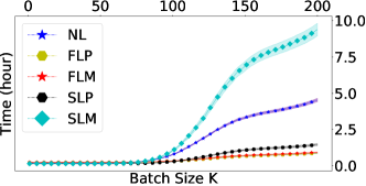
(b) Scalability

Figure 1: (a) Summary of real datasets. Columns $N$, $d$, $|\mathcal{A}|$, and $|\mathcal{C}|$ indicate the number of samples, the dimension, the number of absolute labels, and the number of comparisons, respectively. Column $|\mathcal{C}_{\texttt{trn}}|$ is size of train comparison set, while $T_{\texttt{n}}$ is the execution time under NG for $\mathcal{S}\subseteq\mathcal{C}_{\texttt{trn}},|\mathcal{S}|=200$. Columns $A_{\texttt{ab}},A_{\texttt{ac}}$, indicate the test set AUC of absolute and comparison labels, respectively, when $\mathcal{S}=\mathcal{C}_{\texttt{trn}}$; we report these only for datasets for which we have comparisons. Finally, $\lambda$ is the positive value in Eq. (3.2). For Netflix and Camra, we indicate value ranges across 150 users as appropriate; for MSLR, we report ranges for 150 queries. (b) Scalability of Lazy Greedy Algorithm. Time execution result for large synthetic dataset with $N=15000$, $d=400$, and $|\mathcal{C}|=1.125\times 10^{8}$.

We use synthetic and real datasets to evaluate the performance of different greedy and lazy greedy algorithms. We evaluate these algorithms both in terms of execution time and classification performance w.r.t. accuracy of predictions, after labels are collected.

6.1 Evaluation Setup.

We begin by describing our evaluation setup.

Datasets. In our synthetic dataset, the absolute feature vectors $\bm{x}_{i}\in\mathbb{R}^{d}$, $i\in\mathcal{N}$, are sampled from a Gaussian distribution $\mathtt{N}(\bm{0},\sigma_{x}I_{d})$ with feature dimension $d$ ranging from $20$ to $400$ and dataset size $N$ ranging from $500$ to $15000$. We also sample a parameter vector $\widetilde{\bm{\beta}}$ from Gaussian distribution $\mathtt{N}(\bm{0},\sigma_{\bm{\beta}}I_{d})$. We generate absolute labels $y_{i}$, $i\in\mathcal{N}$, using Eq. (3.3) with $\bm{\beta}=\widetilde{\bm{\beta}}/C_{a}$, where $C_{a}$ is a positive scalar. Finally, we generate $|\mathcal{C}|$ comparison labels via Eq. (3.4), with $\bm{\beta}=\widetilde{\bm{\beta}}$. Parameter $C_{a}$ allows us to control the relative noise ratio between absolute and comparison labels; we set it to $C_{a}=1.2$ in our experiments.

We also use seven real-life datasets, summarized in Fig. 1(a). The first four (ROP, Sushi, Netflix, Camra) contain comparison labels; the remaining (ROP5K, SIFT, and Microsoft URL) do not, and are used only for measuring the execution time of our algorithms. A detailed description of all datasets is in Appendix B.

Algorithms. We implement eight greedy algorithms: Naïve Greedy (NG), Factorization Greedy (FG), Scalar Greedy (SG), Naïve Lazy Greedy (NL), Factorization Lazy Greedy with Pre-Computation (FLP), Factorization Lazy Greedy with Memoization (FLM), Scalar Lazy Greedy with Pre-Computation (SLP), and Scalar Lazy Greedy with Memoization (SLM). In each dataset, we set $\lambda$ in (3.2) to about $10^{-5}$ the average norm of feature vectors (see Fig 1(a)).

We also implement the greedy algorithm with Mutual Information (Mut), Fisher Information (Fisher), and Entropy (Ent) objectives, as described in [5] (also reviewed in Appendix C). Finally, we implement a Random (Ran) baseline method, in which the set $\mathcal{S}$ is selected uniformly at random from $\mathcal{C}_{trn}$.

Experiment Setup. In each experiment, we partition the dataset $\mathcal{N}$ into three datasets: a training set $\mathcal{N}_{\mathtt{trn}}$, a test set $\mathcal{N}_{\mathtt{tst}}$, and a validation set $\mathcal{N}_{\mathtt{val}}$. Wherever available, we denote by $\mathcal{C}_{\mathtt{trn}}\subset\mathcal{C}$ the corresponding comparison set restricted to pairs of objects in $\mathcal{N}_{\mathtt{trn}}$. We select a random subset $\mathcal{A}$ from $\mathcal{N}_{\mathtt{trn}}$ whose absolute labels $y_{i}$, $i\in\mathcal{A}$ are presumed revealed to the experimenter. Then we use our greedy algorithms to select $\mathcal{S}\subset\mathcal{C}_{\mathtt{trn}},|\mathcal{S}|=K$. We record the running time $t_{K}$ of each algorithm for different values of $K\in\mathbb{N}$ executed on the training set. For synthetic data, we repeat each experiment 150 times, each time with a different randomly generated dataset; we report average $t_{k}$ values, as well as standard deviations. For real datasets including absolute labels (ROP, Sushi, Netflix, Camra), we also repeat experiments 150 times, each time with a different randomly selected set $\mathcal{A}$.

For both synthetic and real datasets for which we have comparison labels (ROP, Sushi, Netflix, Camra), we collect the $K$ comparison labels from $\mathcal{S}$ and train a model $\bm{\beta}\in\mathbb{R}^{d}$ using the labels in $\mathcal{A}$ and $\mathcal{S}$ via MAP estimation (3.5), and predict both comparison and absolute labels in the test set. In doing so, we select the parameter $\lambda$ in (3.5) as the value that maximizes AUC on the validation set. Especially, for ROP, we measure the performance w.r.t. the reference standard diagnosis (RSD) label prediction rather than absolute labels, even though the model is trained on (noisier) absolute labels. For each dataset, we perform cross validation, repeating the partition to training and test datasets and keeping the validation set fixed. To produce confidence intervals, each 4-fold cross validation is repeated 150 times, i.e., over 150 different random data shuffles (for the Netflix dataset, the experiment is executed for 150 users).

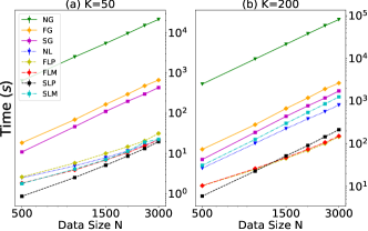
Figure 2: Average execution time for synthetic data under different sample sizes $N$, with feature dimension $d=400$ and $K$ set to $K=50$ in subfigure (a) and $K=200$ in subfigure (b).

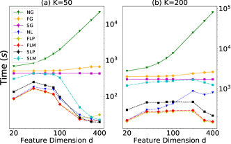
Figure 3: Average execution time for synthetic data under different feature dimensions $d$, with sample size $N=3000$ and $K$ set to $K=50$ in subfigure (a) and $K=200$ in subfigure (b).

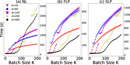
Figure 4: Average execution time as a function of $K$ on synthetic data with $N=5000$ for three lazy greedy algorithms.

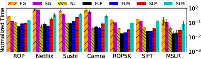
Figure 5: Execution time for different datasets and different algorithms, normalized by NG execution time (see col. $T_{n}(s)$ in Fig. 1(a)).

6.2 Execution Time Performance.

We first study the execution time in terms of $N$, $d$, and $K$.

Dependence on $N$. In Fig. 2 we plot the running time as a function of the data size $N$ for synthetic datasets. The quadratic–$O(N^{2})$–scaling of all algorithms is clearly evident, although the actual execution time varies drastically between different algorithms. Both FG and SG improve upon NG by almost two orders of magnitude. Lazy algorithms improve over NG by as much as 3 orders of magnitude when $K=50$. However, scalar lazy greedy with memoization (SLM) performs similarly to FG and SG when $K=200$, even worse than NL.

Almost universally, pre-processing versions (FLP and SLP) outperform the corresponding memoized versions of the lazy algorithms (FLM and SLM). This is because pre-computation involves a matrix-vector multiplication: in python’s NumPy library this is performed in C language, and is more efficient than the python for-loop inherent in memoization. This negates any benefit of computing only the values needed via memoization. Finally, SLP is the best performer when $K=50$, while FLP outperforms it for large $N$ when $K=200$.

Dependence on $d$. Fig. 3 shows performance over synthetic datasets as a function of dimension $d$. The advantage of FG and SG over the naïve algorithm (NG) is clearly evident: the latter grows super-linearly in $d$. In contrast, the effect of $d$ on FG is linear, while on SG it is almost imperceptible. A striking difference in behavior is observed in the lazy greedy algorithms, that are very sensitive to $d$. Indeed, these algorithms perform poorly in lower dimensions, with the gap between performance for low to high dimensions being sometimes close to two orders of magnitude. This is because, for high $d$, there is are many new dimensions to discover; as a result, almost maximal elements in the heap remain almost maximal in subsequent iterations, leading to early loop terminations. In contrast, in low $d$, maximality changes drastically between iterations, leading to full loop executions.

Dependence on $K$. We further explore this phenomenon in Fig. 4, that shows the dependence of lazy algorithm on $K$. We observe a ‘jump’ in execution time, indicating an expensive loop execution that contributes highly to the execution cost. The smaller $d$ is, the earlier this jump is observed.

Scalability. All in all, we observe that our accelerations, on both standard and lazy greedy algorithms, can significantly reduce the execution time of experimental design. In Fig. 1(b), we illustrate this by running the accelerated lazy algorithms for a large synthetic dataset with $N=15000$ and $d=400$, containing more than $10^{8}$ comparison pairs. The running time of Naïve Greedy (NG) on this dataset exceeds 10 days. As seen in Fig. 1, the running time can be shortened to less than $1$ hour under the Factorization Lazy (FLP) algorithm. We also observe that SLM performs worse than NL, while SLP outperforms NL, again due to the advantage of matrix-vector multiplications over python for-loops.

Time Performance Evaluation on Real Datasets. Experiments on the seven real datasets further corroborate observations made over synthetic data. Fig. 5 shows the execution time normalized by the execution time of NG for each dataset (see column $T_{n}(s)$ in Fig. 1(a)). All algorithms yield an improvement. Lazy greedy algorithms perform well overall, but for the Sushi, CAMRa, and Netflix datasets, this improvement is diminished due to their low dimension $d$. The highest improvement in all algorithms compared to NG is observed in the largest of our datasets, ROP5K, where FG and SG yield an improvement of 1 order of magnitude, while SLP performs exceedingly well, leading to an improvement of 2 orders of magnitude over NG. Overall, FLP consistently improves performance over NL.

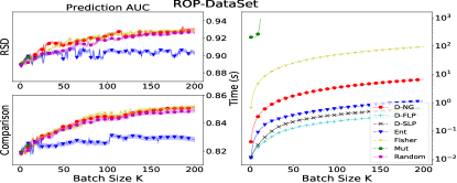
Figure 6: Test set AUC and execution time for ROP dataset, when comparisons samples are selected via D-optimal, Fisher, Entropy and Random and Mutual Information. The classifier is trained via MAP (3.5) on the training set. The left top figure is the test AUC for RSD label, the left bottom figure is the test AUC for comparison labels. The right figure is the execution time for different algorithms. For the D-optimal objective, we record the execution time for Naive Greedy, Factorization Lazy and Scalar Lazy Greedy Algorithm. We only execute Mutual Information for $K\leq 12$.

6.3 Prediction Performance

All 8 algorithms using D-Optimality as an objective produce the same selected set $\mathcal{S}$ (namely, the one determined by the greedy algorithm). We give some intuition of the quality of the model learned via MAP estimation (3.5) in comparison to competitors. This selection has been known to outperform competitors such as Fisher Information and Entropy objectives [5]. For the sake of completeness, we show in Fig. 6 the prediction quality of the resulting trained model w.r.t AUC of both absolute and comparison labels over the test set, on the ROP dataset. Remaining datasets for which we have comparison labels (Sushi, Netflix, and Camra) are shown in Appendix D. In all cases, estimators learned over labels collected by the greedy algorithm significantly outperform random selection. Fisher Information and Mutual Information are sometimes better, but are also exceedingly time consuming, between $10^{2}-10^{3}$ times slower than D-optimal NG. Finally, Entropy is fast, but the prediction performance is not as good as under NG.

We observe similar performance in the remaining datasets, shown in Appendix D. For the Netflix and Camra datasets, we can only scale Mutual Information and Fisher Information to $K\leq 10$, as their complexity is $O(N^{2}2^{K})$ and $O(N^{4}K)$, respectively. In the Sushi and Netflix dataset, the best AUC comes from the D-optimal design algorithm. For the ROP dataset, the D-optimal and Fisher information outperform random for all batch sizes. For the Camra dataset, as $d=10$, the D-optimal design algorithm outperforms Random only when the batch size is less than 100. Finally, Entropy is time efficient but has worse accuracy than all other methods. Our D-optimal Naïve Greedy and its variants have good accuracy and are time-efficient; accelarated methods FLP and SLP are even faster than Entropy.

7 Conclusion

We have shown that experimental design for pairwise comparisons under the D-optimality criterion can be significantly accelerated by exploiting the underlying geometry of pairwise comparisons. Given the prevalence of submodularity in batch active learning objectives, it would be interesting to identify methods through which these results could extend to other objectives of interest. These include objectives that are structurally similar (such as A-optimality or E-optimality [11]), as well as objectives like mutual information, for which even the function value oracle is not tractable.

8 Acknowledgement

Our work is supported by NIH (R01EY019474, P30EY10572), NSF (SCH-1622542 at MGH; SCH-1622536 and CCF-1750539 at Northeastern; SCH-1622679 at OHSU), and by unrestricted departmental funding from Research to Prevent Blindness (OHSU).

A Accelerating the Lazy Greedy Algorithm

Algorithm 5 Lazy Greedy Algorithm

Lazy Greedy Algorithm, as described in Sec. 5. The main Greedy procedure, as well as UpdateS, are the same as in Alg. 1. Tuples are ordered lexicographically.

1:procedure PreProcessing($\mathbf{X}$)

2:    For all $e\in\Omega$, insert tuples $(\Delta(e|\emptyset),e)$ into heap $\mathbf{H}$; Set $\mathcal{S}=\emptyset$.

3:end procedure

1:procedure FindMax($\mathcal{S}$)

2:    while $\mathbf{True}$ do

3:       $(\Delta_{\texttt{old}},e)=$$\mathbf{H}$.PopMax()

4:       Set $\Delta=\textsc{UpdateMarginal}(e,S)$

5:       $(\Delta^{\prime},e^{\prime})=\mathbf{H}.$Max()

6:       if $\Delta\geq\Delta^{\prime}$ then return e

7:       else

8:          $\mathbf{H}$.Insert$\big{(}(\Delta,e)\big{)}$

9:       end if

10:    end while

11:end procedure

1:procedure UpdateMarginal($e,S$)

2:    return $\Delta(e|\mathcal{S})$

3:end procedure

We can employ the same optimizations we describe in Sec. 4 to also accelerate the lazy greedy algorithm. Before describing these optimizations, we briefly review the algorithm below. Intuitively, the lazy greedy algorithm exploits the following fact: by submodularity, for any sets $\mathcal{S^{\prime}}\subseteq\mathcal{S}\subseteq\Omega$ and any $e\in\Omega$ we have that $\Delta(e|\mathcal{S})\leq\Delta(e|\mathcal{S}^{\prime}).$ Every iteration of the greedy algorithm produces a set $\mathcal{S}$ that is a superset of the selected sets $\mathcal{S}^{\prime}$ at all previous iterations. As a result, marginal gains $\Delta(e|\mathcal{S}^{\prime})$ at any previous iteration serve as upper bounds on marginal gains $\Delta(e|\mathcal{S})$ in the current iteration. Thus, to discover $e^{*}$, it suffices to find an element whose current marginal $\Delta(e|\mathcal{S})$ exceeds all past marginal gains: if such an $e$ is found, the loop can terminate early.

The above observation leads to the lazy greedy algorithm in Alg. 5. Past marginal gains are stored in a heap [39]. To find $e^{*}$, the algorithm pops the maximal element $e$ from the heap, and computes its present marginal gain $\Delta(e|\mathcal{S})$. If this exceeds the gain of the (next) maximal element in the heap, then $e$ is $e^{*}$: this is because all values in the heap are upper bounds on the true marginal gains. The loop can thus return $e$ and terminate early. Otherwise, $e$ is placed back in the heap with its (updated) $\Delta(e|S)$, and the process repeats.

Under the value oracle model, the complexity of the lazy greedy algorithm is in fact worse than the standard greedy algorithm: the worst-case cost of an iteration is $O(|\Omega|\log|\Omega|)$, due to heap operations. Though no amortized complexity results are known, in practice loops often terminate early; this leads to a significant computational improvement in a broad array of problems [40, 41, 42, 43] and motivates us to apply our accelerations to lazy greedy as well. We now describe how the accelerations we presented in Sec. 4 can be incorporated in the lazy greedy algorithm.

Algorithm 6 Naïve Lazy Greedy Algorithm

Naïve Lazy Algorithm, as described in Sec. 5. The main Greedy procedure, as well as UpdateS and FindMax are the same as in Alg. 5.

1:procedure PreProcessing($\mathbf{X}$)

2:    Compute $\mathbf{A}_{0}^{-1}=(\lambda I_{d}+\underset{i\in\mathcal{A}}{\sum}\bm{x}_{i}\bm{x}_{i}^{T})^{-1}$; Set $\mathbf{A}^{-1}=\mathbf{A}_{0}^{-1}$

3:    For all $e\in\Omega$, insert tuples $(\bm{x}_{e}^{T}\mathbf{A}^{-1}\bm{x}_{e},e)$ into heap $\mathbf{H}$; Set $\mathcal{S}=\emptyset$.

4:end procedure

1:procedure UpdateMarginal($e,S$)

2:    return $\bm{x}_{e}^{T}\mathbf{A}^{-1}\bm{x}_{e}$

3:end procedure

Naïve Lazy Greedy. To begin with, we can exploit the same simple improvements we described in Sec. 4.1: rather than storing the marginal gains $\Delta(e|\mathcal{S})$, the–simpler to compute–quantities $d_{e}$, given by (4.10), can be stored in the heap instead. Matrix $\mathbf{A}^{-1}$, can again be updated via the Sherman-Morisson formula (4.11). Both are straightforward to implement; see Alg. 6 for pseudocode.

Algorithm 7 Factorization Lazy Greedy Algorithm

Factorization Lazy Algorithm, as described in Sec. 5. The main Greedy procedure, as well as FindMax, are the same as in Alg. 5.

1:procedure PreProcessing($\mathbf{X}$)

2:    Compute $\mathbf{A}_{0}^{-1}=(\lambda I_{d}+\underset{i\in\mathcal{A}}{\sum}\bm{x}_{i}\bm{x}_{i}^{T})^{-1}$; Set $\mathbf{A}^{-1}=\mathbf{A}_{0}^{-1}$; Set $\mathcal{S}=\emptyset$

3:    Factorize the matrix $\mathbf{A}^{-1}$ into $\mathbf{A}^{-1}=\mathbf{U}^{T}\mathbf{U}$.

4:    Calculate and save $\bm{z}_{i}=\mathbf{U}\bm{x}_{i}$ for all $i\in\mathcal{N}$.

5:    For all $e\in\Omega$, insert tuples $(||\bm{z}_{i}-\bm{z}_{j}||_{2}^{2},e)$ into heap $\mathbf{H}$.

6:end procedure

1:procedure UpdateMarginal($e,S$)

2:    return $||\bm{z}_{i}-\bm{z}_{j}||_{2}^{2}$

3:end procedure

1:procedure UpdateS($\mathcal{S},e^{*}$)

2:    $\mathcal{S}=\mathcal{S}\cup e^{*}$; $\mathbf{A}^{-1}=\mathbf{A}^{-1}-\frac{\mathbf{A}^{-1}\bm{x}_{e^{*}}\bm{x}_{e^{*}}^{T}\mathbf{A}^{-1}}{1+\bm{x}_{e^{*}}^{T}\mathbf{A}^{-1}\bm{x}_{e^{*}}}$

3:    Factorize the matrix $\mathbf{A}^{-1}$ into $\mathbf{A}^{-1}=\mathbf{U}^{T}\mathbf{U}$.

4:    Pre-compute and save $\bm{z}_{i}=\mathbf{U}\bm{x}_{i}$ for all $i\in\mathcal{N}$.

5:end procedure

Factorization Lazy Greedy. As in Sec. 4.2, prior to the loop in FindMax that locates the maximal element, the matrix $\mathbf{A}^{-1}$ can be factorized as $\mathbf{A}^{-1}=\mathbf{U}^{T}\mathbf{U}$ via Cholesky factorization. Again, vectors $\bm{z}_{i}=\mathbf{U}\mathbf{x}_{i}$, $i\in\mathcal{N}$, can be pre-computed and used in subsequent computations of quantities $d_{e}$ as needed. In theory, as the loop may terminate early, it is best to not precompute a vector $\bm{z}_{i}$, $i\in\mathcal{N}$, but only compute it the first time some $e=(i,j)\in\mathcal{C}$, is popped from the heap, and the computation of $d_{e}$ requires it. Once a $\bm{z}_{i}$, $i\in\mathcal{N}$ has been computed thusly, it can be re-used again in subsequent comparison pairs $(i,j^{\prime})\in\mathcal{C}$ that require it. We call this algorithm Factorization-Lazy-Greedy with Memoization, as $\bm{z}_{i}$ computations are memoized (i.e., computed as needed and saved to be used later). In practice (see Sec. 6), pre-computing all $\mathbf{z}_{i}$, $i\in\mathcal{N}$, even if they are not all used in the subsequent lazy loop evaluation, and paying the corresponding $O(Nd^{2})$ cost may be faster when matrix-vector multiplications are optimized; we call this algorithm Factorization Lazy Greedy with Pre-Computation. We elaborate on this in Sec. 6, where we implement both versions of the algorithm.

Factorization Lazy Greedy is shown in pseudocode in Alg. 7; we provide only pseudocode for the pre-computed version. In particular, we pre-compute and save $\bm{z}_{i}=\mathbf{U}\bm{x}_{i}$ for all $i\in\mathcal{N}$ in line 4 of procedure UpdateS, paying an $O(Nd^{2})$ cost per iteration. Not all such values are used by the Greedy algorithm however, as a loop may terminate early. In the memoized version, $\bm{z}_{i}$ are computed online/as needed at line 2 of procedure UpdateMarginal, and stored/reused at later calls.

Algorithm 8 Scalar Lazy Algorithm

Lazy Greedy Algorithm, as described in Sec. 5. The main Greedy procedure is the same as in Alg. 1.

1:procedure PreProcessing($\mathbf{X}$)

2:    Compute $\mathbf{A}_{0}^{-1}=(\lambda I_{d}+\underset{i\in\mathcal{A}}{\sum}\bm{x}_{i}\bm{x}_{i}^{T})^{-1}$; Set $\mathbf{A}^{-1}=\mathbf{A}_{0}^{-1}$

3:    Factorize the matrix $\mathbf{A}^{-1}$ into $\mathbf{A}^{-1}=\mathbf{U}^{T}\mathbf{U}$.

4:    Calculate and save $\bm{z}_{i}=\mathbf{U}\bm{x}_{i}$ for all $i\in\mathcal{N}$.

5:    For all $e\in\Omega$, insert tuples $(||\bm{z}_{i}-\bm{z}_{j}||_{2}^{2},0,e)$ into heap $\mathbf{H}$.

6:    Set $\mathcal{S}=\emptyset,k=0$.

7:end procedure

1:procedure FindMax($f,\mathcal{S}$)

2:    while True do

3:       $(\Delta_{\texttt{old}},t,e)=$ $\mathbf{H}$.PopMax()

4:       Set $\Delta=\textsc{UpdateMarginal}(\Delta_{old},t,e,S)$

5:       $(\Delta^{\prime},t,e^{\prime})=\mathbf{H}.$Max()

6:       if $\Delta\geq\Delta^{\prime}$ then return e

7:       else

8:          $\mathbf{H}$.Insert$\big{(}(\Delta,k,e)\big{)}$

9:       end if

10:    end while

11:end procedure

1:procedure UpdateMarginal($\Delta_{\texttt{old}},t,e,S$)

2:    return $\Delta_{\texttt{old}}-\underset{t\leqslant l<k}{\sum}(\rho_{l,i}-\rho_{l,j})^{2}$

3:end procedure

1:procedure UpdateS($\mathcal{S},e^{*}$)

2:    Compute and save $\bm{v}_{k}=\frac{\mathbf{A}^{-1}\bm{x}_{e^{*}}}{\sqrt{1+\bm{x}_{e^{*}}^{T}\mathbf{A}^{-1}\bm{x}_{e^{*}}}}$

3:    Pre-compute and save $\rho_{k,i}=\bm{v}_{k}^{T}\bm{x}_{i}$ for all $i\in\mathcal{N}$.

4:    $\mathbf{A}^{-1}=\mathbf{A}^{-1}-\bm{v}\bm{v}^{T}$

5:    $\mathcal{S}=\mathcal{S}\cup e^{*}$

6:    $k=|\mathcal{S}|$

7:end procedure

Scalar Lazy Greedy. Finally, as in Sec. 4.3, values $d_{e}$ can be adapted using formula (4.13). Beyond maintaining and updating the corresponding variables present in Alg. 4 ( $z_{i}=\bm{v}^{T}\mathbf{x}_{i}$, $i\in\mathcal{N}$, vector $\bm{v}$ given by (4.13), etc.), adapting $d_{e}$ via (4.13) poses a challenge in the context of lazy greedy: this is because the formula provides the adaptation rule w.r.t. the value $d_{e}$ in the immediately preceding iteration. The values $d_{e}$ stored and retrieved (via a pop) from the heap may have been computed at an arbitrarily old iteration. Hence, to construct the (approximate) marginal gain $d_{e}$ under the current set $S$ from a popped value from the heap we may need to repeatedly apply (4.13) more than once. This requires to also keep track the iteration at which tuples are inserted in the heap, so that the appropriate vectors $\bm{v}$ can be used to adapt them. We indeed track this information in Alg. 8.

We note that, as a result, the execution of UpdateMarginal may be quite expensive when popped values of the heap are quite “stale” (i.e., were computed in very early iterations). Hence, in contrast to the standard greedy versions of these algorithms, it is not a-priori obvious that Scalar Lazy Greedy always outperforms Factorization Lazy Greedy; we indeed observe the opposite in our experiments in Sec. 6. Finally, as in Factorization Lazy Greedy, multiplications $\bm{v}^{T}\bm{x}_{i}$ can again either be fully pre-computed at each iteration (paying the full $O(Nd)$ cost), or memoized and used as necessary. We again implement and evaluate both options in Sec. 6.

Pseudocode for Scalar Lazy Greedy can be found in Alg. 8. Again, we provide pseudocode only only for the version that uses pre-computation. In particular, quantities $\rho_{k,i}$, for $k\in\{1,\ldots,K\}$, $i\in\mathcal{N}$, are pre-computed at line 4 of UpdateS; in a memoized version, they can again be computed online/as needed at line 2 of UpdateMarginal. Note that, in both cases, this requires computing and saving vectors $\bm{v}_{k}$, that can be used as necessary.

B Real Datasets

We provide here a detailed description of the datasets we use in our experiments.

ROP Dataset. Our first dataset [1] consists of 100 images of retinas, labeled by experts w.r.t. the presence of a disease called Retinopathy of Prematurity (ROP). We represent each image through a vector $\bm{x}_{i}\in\mathbb{R}^{d}$ where $d=156$, using the feature extraction procedure of [1], comprising statistics of several indices such as blood vessel curvature, dilation, and tortuosity. Five experts provide diagnostic labels for all 100 images, categorizing them as Plus, Preplus and Normal. We convert these to absolute labels $y_{i}\in\{-1,+1\}$ by mapping Plus and Preplus as $+1$ and Normal to $-1$. Finally, these five experts also provide $|\mathcal{C}|=29705$ comparison labels for 4950 pairs of images in this dataset. Beyond these labels, we also have Reference Standard Diagnosis (RSD) labels for each of these images, which are created via a consensus reached by a committee of 3 experts. We use these additional labels for testing purposes, as described below.

ROP5K Dataset. The ROP5K dataset [44] consists of $N=5000$ unlabeled images of retinas. Each image has a feature dimension $d=143$, generated again via the feature extraction process of [1]. We execute 150 experiments on random samples of size $N=3000$ from this dataset, and report performance averages.

SUSHI Dataset. The SUSHI Preference dataset [45] consists of rankings of $N=100$ sushi food items by 5000 customers. Each customer ranks 10 items according to her preferences. Each sushi item is associated with a feature vector $\bm{x}_{i}\in\mathbb{R}^{d}$ where $d=20$, consisting of features such as style, group, heaviness/oiliness in taste, frequency, and normalized price. We generate comparison labels as follows. For any pair of items $i,j\in\mathcal{N}$ in a customer’s ranked list, if $i$ precedes $j$ in the list, we set $y_{i,j}=+1$, otherwise, $y_{i,j}=-1$. We also produce absolute labels via the Elo ranking algorithm [46]. This gives us an individual score for each item; we convert the individual score to an absolute label $y_{i}\in\{-1,+1\}$ by setting items above (below) the median score to $+1$ ($-1$).

Netflix Dataset. The Netflix dataset has multiple users and $17770$ movies. We select 150 users who have rated more than 833 movies. Each movie has a 30-dimensional vector obtained via matrix factorization [47] over the entire dataset. We generate binary absolute labels as follows: if the rate score is above (below) the user mean, the absolute label is $+1$ ($-1$). If the scores between two movies $i$ and $j$ are different, we generate comparison label $y_{i,j}=+1$ if score $i$ is higher than score $j$, otherwise we break ties by setting $y_{i,j}=-1$.

MSLR Dataset. The MSLR-WEB10K dataset [48] has $10000$ queries. The datasets consist of $134$-dimensional features such as covered query term number, covered query term ratio, stream length, inverse document frequency (IDF), etc. We restrict the dataset to 150 queries submitted more than 325 times.

SIFT dataset. The SIFT10M dataset [49] has often been used for evaluating the approximate nearest neighbour search methods. Each data point is a SIFT feature which is extracted from Caltech-$256$ by the open source VLFeat library. The dataset has a total of 11164866 instances and each SIFT feature has a dimensionality of 128. We execute 150 experiments on random samples of size $N=3000$ in this dataset, and report performance averages.

CAMRa Dataset. The CAMRa dataset [50] has multiple users and $23893$ movies. We select 150 users who have rated more than 896 movies. Each movie has a 10-dimensional vector obtained via matrix factorization over the entire dataset.

C Competitor Methods

We implement the greedy algorithm with the following objectives (see also [5]):

Mutual Information. Recall that the prior distribution is $\bm{\beta}\sim\mathcal{N}(0,\sigma^{2}I_{d})$. The objective function is to maximize the mutual information between the parameter vector $\bm{\beta}$ and selected comparison labels $Y_{\mathcal{S}}$, conditioned on the observed absolute labels, i.e:

(C.1) $$\begin{split}f_{1}(\mathcal{S})=&\mathbf{I}(\bm{\beta};Y_{\mathcal{S}}|Y_{\mathcal{A}}=y_{\mathcal{A}})\\ =&\mathbf{H}(Y_{\mathcal{S}}|Y_{\mathcal{A}}=y_{\mathcal{A}})-\mathbf{H}(Y_{\mathcal{S}}|\bm{\beta},Y_{\mathcal{A}}=y_{\mathcal{A}}),\end{split}$$

where $\mathbf{I}(\cdot|Y_{\mathcal{A}}=y_{\mathcal{A}})$ denotes the mutual information conditioned on the observed absolute labels and $\mathbf{H}(\cdot|Y_{\mathcal{A}}=y_{\mathcal{A}})$ denotes the entropy conditioned on the observed absolute labels. We compute the quantities in Eq. (C.1) using the Bradley-Terry generative model described in (3.4).

Information Entropy. Recall that given some observed absolute labels $y_{\mathcal{A}}$, we can estimate the parameter vector $\hat{\bm{\beta}}$ by:

(C.2) $$\begin{split}\hat{\bm{\beta}}=\textstyle\mathop{\mathbf{argmax}}_{\bm{\beta}}\mathcal{L}(\bm{\beta};\mathcal{A},\emptyset),\end{split}$$

where the negative log-likelihood function $\mathcal{L}(\bm{\beta};\mathcal{A},\mathcal{S})$ is given by Eq. (3.5). Under our generative model, unlabeled samples are independent given $\hat{\bm{\beta}}$; hence, the information entropy objective can be written as:

(C.3) $$f_{2}(\mathcal{S})=\textstyle\mathbf{H}(Y_{\mathcal{S}}|\bm{\beta}=\hat{\bm{\beta}})=\sum_{a\in\mathcal{S}}\mathbf{H}(Y_{a}|\bm{\beta}=\hat{\bm{\beta}}).$$

Assuming that the experimenter estimates the parameter vector $\hat{\bm{\beta}}$, thus we can use information entropy to measure the unpredictability of $Y_{\mathcal{S}}$ . This can be seen as a “point” estimate of the mutual information.

Fisher Information. The Fisher information measures the amount of information that an observable random feature $\bm{x}$ carries about an unknown parameter $\bm{\beta}$ upon which the probability of $\bm{x}$ depends. The Fisher information matrix can be written as:

(C.4) $$\textstyle I(\bm{\beta})=-\int p(y|\bm{x},\bm{\beta})\frac{\partial^{2}}{\partial\bm{\beta}^{2}}\mathop{\log}p(y|\bm{x},\bm{\beta})\mathrm{d}\bm{x}\mathrm{d}y.$$

Let $p(\bm{x})$ be the feature distribution of all unlabeled examples in set $\mathcal{C}$ and $q(\bm{x})$ be the distribution of unlabeled examples in set $\mathcal{S}$ that are chosen for manual labeling. With the generative model and the estimation of parameter vector $\hat{\bm{\beta}}$ by Eq. (C.2), the Fisher information matrices for these two distributions can be written as:

$$\begin{split}I_{p}(\hat{\bm{\beta}})&=\textstyle\frac{1}{|\mathcal{C}|}{\sum}_{(i,j)\in\mathcal{C}}\pi(\bm{x}_{i,j})(1-\pi(\bm{x}_{i,j}))\bm{x}_{i,j}\bm{x}_{i,j}^{T}+\delta I_{d},\\ I_{q}(\mathcal{S},\hat{\bm{\beta}})&=\textstyle\frac{1}{|\mathcal{S}|}{\sum}_{(i,j)\in\mathcal{C}}\pi(\bm{x}_{i,j})(1-\pi(\bm{x}_{i,j}))\bm{x}_{i,j}\bm{x}_{i,j}^{T}+\delta I_{d},\end{split}$$

where $\delta\ll 1$ is to avoid having a singular matrix,
$\pi(\bm{x}_{i,j})=\frac{1}{1+\mathop{\exp}(-\bm{\beta}^{T}\bm{x}_{i,j})},$ for $(i,j)\in\mathcal{C}$, and $\bm{x}_{i,j}=\bm{x}_{i}-\bm{x}_{j}$. The matrices above relate to variance of the parameter estimate via the so-called Cramer-Rao bound maximizing

(C.5) $$f_{4}(\mathcal{S})=-\mathop{\mathrm{tr}}(I_{q}(\mathcal{S},\hat{\bm{\beta}})^{-1}I_{p}(\hat{\bm{\beta}}))$$

minimizes the Cramer-Rao bound of the respective $\hat{\bm{\beta}}$.

D Accuracy $\&$ Time Efficiency vs Competitors

Here, we provide the accuracy and time efficiency result for the Sushi, Netflix and Camra datasets. For Figure. 7 to 9, we show the accuracy and time efficiency for both D-optimal design and competitors on Sushi, Netflix and Camra datasets. We reach the same conclusion as the ones reported in Sec. 6. We note that, for the Netflix and Camra datasets, we can only compute a batch size less than ten for Fisher Information and Mutual Information. This is because the Mutual has a complexity $O(N^{2}2^{K})$ and Fisher has a complexity $O(N^{4}K)$. In the Sushi and Netflix dataset, the best AUC comes from the D-optimal design algorithm. For the Camra dataset, as the dimension is only ten, the D-optimal design algorithm can only beat Random when the batch size is less than 100. The Entropy method is time efficient but has worse accuracy than other methods. The D-optimal Naive Greedy and its variant have good accuracy and are time efficient and after the acceleration FLP and SLP are even faster than Entropy method.

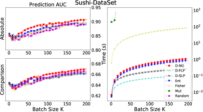
Figure 7: Test set AUC and execution time for Sushi dataset, when comparisons samples are selected via D-optimal, Fisher, Entropy and Random and Mutual Information. The classifier is trained via MAP (3.5) on the training set. The left figure is the test AUC for absolute label, the middle figure is the test AUC for comparison labels. The right figure is the execution time for different algorithms. Especially, for the D-optimal method we record the execution time for Naive Greedy, Factorization Lazy and Scalar Lazy Greedy Algorithm. For Mutual information we only execute it for batch size no more than 12.

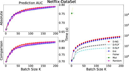
Figure 8: Test set AUC and execution time for Netflix dataset, when comparisons samples are selected via D-optimal, Fisher, Entropy and Random and Mutual Information. The classifier is trained via MAP (3.5) on the training set. The left figure is the test AUC for absolute label, the middle figure is the test AUC for comparison labels. The right figure is the execution time for different algorithms. Especially, for the D-optimal method we record the execution time for Naive Greedy, Factorization Lazy and Scalar Lazy Greedy Algorithm. For Mutual information we only execute it for batch size no more than 8, for Fisher information method we only execute it for batch size no more than 5.

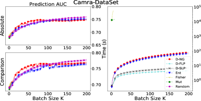
Figure 9: Test set AUC and execution time for Camra dataset, when comparisons samples are selected via D-optimal, Fisher, Entropy and Random and Mutual Information. The classifier is trained via MAP (3.5) on the training set. The left figure is the test AUC for absolute label, the middle figure is the test AUC for comparison labels. The right figure is the execution time for different algorithms. Especially, for the D-optimal method we record the execution time for Naive Greedy, Factorization Lazy and Scalar Lazy Greedy Algorithm. For Mutual information we only execute it for batch size no more than 8, for Fisher information method we only execute it for batch size no more than 5.

References

- [1] J. K-Cramer, J. P. Campbell, D. Erdogmus, et al. Plus disease in retinopathy of prematurity: improving diagnosis by ranking disease severity and using quantitative image analysis. Ophthalmology, 2016.
- [2] D. Sculley. Combined regression and ranking. In KDD, 2010.
- [3] M. S. Desarkar, S. Sarkar, and P. Mitra. Aggregating preference graphs for collaborative rating prediction. In Recsys, 2010.
- [4] M. S. Desarkar, R. Saxena, and S. Sarkar. Preference relation based matrix factorization for recommender systems. In UMAP, 2012.
- [5] Y. Guo, P. Tian, J. Kalpathy-Cramer, S. Ostmo, J. P. Campbell, M. F. Chiang, D. Erdogmus, J. Dy, and S. Ioannidis. Experimental Design Under the Bradley-Terry Model. In IJCAI, 2018.
- [6] N. Stewart, G. DA Brown, and N. Chater. Absolute identification by relative judgment. Psychological Review, 2005.
- [7] A. Brun, A. Hamad, O. Buffet, and A. Boyer. Towards preference relations in recommender systems. In ECML/PKDD, 2010.
- [8] Y. Zheng, L. Zhang, X. Xie, and Wei-Ying Ma. Mining interesting locations and travel sequences from GPS trajectories. In WWW. ACM, 2009.
- [9] Y. Koren and J. Sill. OrdRec: an ordinal model for predicting personalized item rating distributions. In Recsys, 2011.
- [10] M. Schultz and T. Joachims. Learning a distance metric from relative comparisons. In NIPS, 2004.
- [11] S. Boyd and L. Vandenberghe. Convex optimization. Cambridge university press, 2004.
- [12] F. Pukelsheim. Optimal design of experiments. SIAM, 1993.
- [13] G. L. Nemhauser, L. A. Wolsey, and M. L Fisher. An analysis of approximations for maximizing submodular set functions. Mathematical Programming, 1978.
- [14] G. H. Golub and C. F. Van Loan. Matrix computations. JHU Press, 2012.
- [15] J. Sherman and W. J. Morrison. Adjustment of an inverse matrix corresponding to a change in one element of a given matrix. Ann. Math. Stat, 1950.
- [16] M. Minoux. Accelerated greedy algorithms for maximizing submodular set functions. In Optimization techniques. 1978.
- [17] B. Mirzasoleiman, A. Badanidiyuru, A. Karbasi, J. Vondrák, and A. Krause. Lazier Than Lazy Greedy. In AAAI, 2015.
- [18] H. Lin and J. Bilmes. A class of submodular functions for document summarization. In HLT, 2011.
- [19] B. Mirzasoleiman, A. Karbasi, R. Sarkar, and A. Krause. Distributed submodular maximization: Identifying representative elements in massive data. In NIPS, 2013.
- [20] L. Chen, P. Zhang, and B. Li. Fusing pointwise and pairwise labels for supporting user-adaptive image retrieval. In ICMR, pp 67–74, 2015.
- [21] H. Takamura and J. Tsujii. Estimating numerical attributes by bringing together fragmentary clues. In HLT, 2015.
- [22] Y. Wang, S. Wang, J. Tang, H. Liu, and B. Li. PPP: Joint pointwise and pairwise image label prediction. In CVPR, 2016.
- [23] J. Liepe, S. Filippi, M. Komorowski, and M. P. Stumpf. Maximizing the information content of experiments in systems biology. PLOS Comput. Biol, 2013.
- [24] D. R. Cavagnaro, J. I. Myung, M. A. Pitt, and J. V. Kujala. Adaptive design optimization: A mutual information-based approach to model discrimination in cognitive science. Neural computation, 2010.
- [25] A. Krause and C. E. Guestrin. Near-optimal nonmyopic value of information in graphical models. arXiv preprint arXiv:1207.1394, 2012.
- [26] A. G. Busetto, A. Hauser, G. Krummenacher, M. Sunnåker, S. Dimopoulos, C. S. Ong, Jö. Stelling, and J. M. Buhmann. Near-optimal experimental design for model selection in systems biology. Bioinformatics, pp 2625–2632, 2013.
- [27] A. Krause and D. Golovin. Submodular function maximization., 2014.
- [28] D. Golovin and A. Krause. Adaptive submodularity: Theory and applications in active learning and stochastic optimization. JAIR, 2011.
- [29] K. G. Jamieson and R. Nowak. Active ranking using pairwise comparisons. In NIPS, 2011.
- [30] U. Graßhoff and R. Schwabe. Optimal design for the Bradley–Terry paired comparison model. Statistical Methods and Applications, 2008.
- [31] M. E. Glickman and S. T. Jensen. Adaptive paired comparison design. Journal of statistical planning and inference, pp 279–293, 2005.
- [32] R. A. Bradley and M. E. Terry. Rank analysis of incomplete block designs: I. The method of paired comparisons. Biometrika, 1952.
- [33] X. He. Laplacian regularized D-optimal design for active learning and its application to image retrieval. IEEE Transactions on Image Processing, 2010.
- [34] D. A. Harville. Matrix algebra from a statistician’s perspective. Springer, 1997.
- [35] W. H. Press. Numerical recipes 3rd edition: The art of scientific computing. Cambridge university press, 2007.
- [36] J. Leskovec, A. Krause, C. Guestrin, C. Faloutsos, J. VanBriesen, and N. Glance. Cost-effective outbreak detection in networks. In KDD, 2007.
- [37] A. Krause and C. Guestrin. Near-optimal observation selection using submodular functions. In AAAI, 2007.
- [38] Z. Changshui, H. Guangdong, and W. Jun. A fast algorithm based on the submodular property for optimization of wind turbine positioning. Renewable Energy, 2011.
- [39] M. Liu, O. Tuzel, S. Ramalingam, and R. Chellappa. Entropy rate superpixel segmentation. In CVPR, 2011.
- [40] M. Gomez-Rodriguez, J. Leskovec, and A. Krause. Inferring networks of diffusion and influence. TKDD, 2012.
- [41] G. Calinescu, C. Chekuri, M. Pál, and J. Vondrák. Maximizing a monotone submodular function subject to a matroid constraint. SIAM Journal on Computing, 2011.
- [42] A. Krause, A. Singh, and C. Guestrin. Near-optimal sensor placements in Gaussian processes: Theory, efficient algorithms and empirical studies. JMLR, 2008.
- [43] Q. Sun and D. Batra. Submodboxes: Near-optimal search for a set of diverse object proposals. In NIPS, 2015.
- [44] J. M. Brown, J. P. Campbell, A. Beers, K. Chang, K. Donohue, S. Ostmo, RV. P. Chan, J. Dy, D. Erdogmus, S. Ioannidis, et al. Fully automated disease severity assessment and treatment monitoring in retinopathy of prematurity using deep learning. In Medical Imaging, 2018.
- [45] T. Kamishima, M. Hamasaki, and S. Akaho. A simple transfer learning method and its application to personalization in collaborative tagging. In ICDM, 2009.
- [46] A. E. Elo. The rating of chessplayers past and present. Arco Pub, 1978.
- [47] Y. Koren, R. Bell, and C. Volinsky. Matrix factorization techniques for recommender systems. Computer, 2009.
- [48] Tao Qin and Tie-Yan Liu. Introducing LETOR 4.0 Datasets. CoRR, abs/1306.2597, 2013.
- [49] D. Dheeru and E. Karra Taniskidou. UCI Machine Learning Repository, 2017.
- [50] J. Bento, N. Fawaz, A. Montanari, and S. Ioannidis. Identifying users from their rating patterns. In CAMRa, 2011.