Vacuum energy decay from a q-bubble

Abstract

We consider a finite-size spherical bubble with a nonequilibrium value of the $q$-field, where the bubble is immersed in an infinite vacuum with the constant equilibrium value $q_{0}$ for the $q$-field (this $q_{0}$ has already cancelled an initial cosmological constant). Numerical results are presented for the time evolution of such a $q$-bubble with gravity turned off and with gravity turned on. For small enough bubbles and a $q$-field energy scale sufficiently below the gravitational energy scale $E_{\text{Planck}}$, the vacuum energy of the $q$-bubble is found to disperse completely. For large enough bubbles and a finite value of $E_{\text{Planck}}$, the vacuum energy of the $q$-bubble disperses only partially and there occurs gravitational collapse near the bubble center.

I Introduction

The energy density of the vacuum, the dark energy, and the cosmological constant are highly debated topics today, as quantum field theory suggests a typical number that is some 120 orders of magnitude larger Zeldovich1968 ; Weinberg1988 than what has been observed Tanabashi-etal2018 . The mismatch is so large and so significant as to make it the main outstanding problem of modern physics. However, a similar vacuum energy problem exists in condensed-matter systems, and its solution may provide a hint for the solution of the cosmological constant problem. In condensed matter, the zero-point energy of the quantum fields is fully cancelled by the microscopic (atomic) degrees of freedom, if the system is in its ground state. If the system is slightly out of equilibrium, the vacuum energy is not fully compensated, but its magnitude is determined by the infrared energy scale rather than by the ultraviolet (atomic) energy scale.

Still, in order to apply this condensed-matter scenario of the cancellation of the vacuum energy to the quantum vacuum of our Universe, we need to know the proper variables to describe this quantum vacuum. One example of such a variable is the four-form field strength used by Hawking in particular Hawking1984 . The nonlinear extension of this approach, which goes under the name of $q$-theory KV2008a ; KV2008b ; KV2016-Lambda-cancellation , demonstrates the nullification of the vacuum energy density in a full-equilibrium vacuum without matter present. A small cosmological constant appears if the vacuum is out of equilibrium. Its value is then determined by infrared physics and is proportional either to the matter content of the Universe or to the Hubble expansion rate.

While $q$-theory solves the main cosmological problem (other realizations of the $q$ variable are presented in Refs. KlinkhamerVolovik2016-brane ; KlinkhamerVolovik2018-tetrads and a one-page review appears as App. A in Ref. KlinkhamerVolovik2011-JPCS ), the dynamical process of equilibration of the vacuum towards the full equilibrium is still under investigation. The previously obtained results KV2008b concern the decay of an initially homogeneous high-energy state emerging immediately after the Big Bang. These calculations demonstrated that, with generic initial conditions, the high-energy state prefers to relax to a de-Sitter vacuum rather than to the Minkowski vacuum. On the other hand, the possibility of the final decay of the de-Sitter vacuum to the Minkowski vacuum is under intensive debate. This is because of the special symmetry of de-Sitter spacetime; see, e.g., Refs. Markkanen2018 ; Matsui2018 and references therein.

One way to circumvent this de-Sitter controversy is to consider the case that the Big Bang takes place not over the whole of space but only in a finite region of space, which is surrounded by equilibrium Minkowski vacuum. This possibility is also suggested by condensed-matter experiments Ruutu-etal1996 , where a hot spot created within the equilibrium state finally relaxes to the full equilibrium by radiating the extra energy away to infinity.

Concretely, we propose to calculate, in the $q$-theory framework KV2008a ; KV2008b , the time evolution of a finite-size spherical bubble with $q\neq q_{0}$, which is immersed in an infinite equilibrium vacuum with $q=q_{0}$, where $q_{0}$ has already cancelled an initial cosmological constant $\Lambda$. The expectation is that the interior field $q(t,\,r)$ relaxes to $q_{0}$, while the bubble wall (or its remnant) ultimately moves outwards. Yet, gravity may hold surprises in store. Remark that our proposed calculation corresponds to the scenario discussed in the second paragraph of Sec. V A in Ref. KV2008b , which mentioned the possibility that “the starting nonequilibrium state could, in turn, be obtained by a large perturbation of an initial equilibrium vacuum.” We emphasize that the calculation of the present article is the first-ever calculation of the inhomogeneous dynamics of the quantum vacuum in the $q$-theory framework.

Before we start with this calculation, we have three clarifying comments. The first comment is that it may be instructive to compare our $q$-bubble to the vacuum bubble as discussed by Coleman and collaborators Coleman1977 ; CallanColeman1977 ; ColemanDeLuccia1980 . That discussion starts from a classical field theory of a fundamental scalar field $\phi(x)$ with nonderivative interactions. The interactions are, in fact, determined by a potential term $V(\phi)$ in the action. The potential $V(\phi)$ is assumed to have various local minima: one or more “false” vacua $\phi_{+,n}$ and the single “true” vacuum $\phi_{-}$, where the “false” vacua have a larger energy density $V(\phi_{+,n})$ than the value $V(\phi_{-})$ of the “true” vacuum. Coleman’s vacuum bubble, then, corresponds to a finite-size spherical bubble with “true” vacuum inside and “false” vacuum outside (in other words, the energy density inside is lower than outside). The dynamic behavior of a single vacuum bubble is that the bubble expands (cf. Fig. 4 in Ref. Coleman1977 ) with the true-vacuum region increasing but, at a given finite time, the far-away region remaining in a false-vacuum state. Such a vacuum bubble is essentially different from our $q$-bubble which has an infinite equilibrium vacuum with $q=q_{0}$ outside (in Coleman’s terminology, “true” $q$-vacuum outside). In a way, the $q$-bubble resembles Coleman’s vacuum bubble with interior and exterior regions switched. It is clear that, already energetically, the dynamic behavior of the $q$-bubble will be different from that of Coleman’s vacuum bubble.

The second comment concerns the different role of a fundamental scalar field $\phi(x)$ and the vacuum variable $q(x)$ for the cosmological constant problem. In the fundamental-scalar-field approach, the nullification of the energy density $\epsilon(\phi)$ in the equilibrium vacuum requires fine-tuning Weinberg1988 . In the $q$-field approach, the vacuum is a self-sustained system, which, in equilibrium, automatically acquires a zero value for the thermodynamic potential $\widetilde{\epsilon}(q)=\epsilon(q)-q\,d\epsilon(q)/dq$ that enters the Einstein equation by a cosmological-constant-type term. See, in particular, the discussion of Sec. 2 in Ref. KlinkhamerVolovik2016-brane .

The third comment expands on the second and concerns the actual dynamics of the $q$-field. At first glance, the dynamical equations used in the present article are identical to the equations of general relativity coupled to a “scalar” field $q(x)$ with a potential $\rho_{V}(q)$ to be defined later. The dynamics of a fundamental scalar field $\phi(x)$ interacting with gravity has been extensively studied, in particular by Choptuik and collaborators Choptuik1993 ; MarsaChoptuik1996 ; HondaChoptuik2002 (see also Refs. Choptuik-etal2015 ; Cardoso-etal2015 for two recent reviews on numerical relativity). In general, however, the $q$-field has only locally the property of a scalar field, while it globally obeys a conservation law. It is precisely this conservation law that makes the four-form field strength appropriate for the description of the phenomenology of the quantum vacuum. All this makes the dynamics of the quantum vacuum essentially different from the dynamics of a fundamental scalar field. This issue will be discussed further in Sec. II.

We, now, turn to the calculation of the time evolution of a $q$-bubble. After a brief review of the theory, we, first, consider a $q$-bubble with gravity effects turned off and, then, with gravity effects turned on. Throughout, we use natural units with $c=\hbar=1$ and take the metric signature $(-+++)$.

II Theory and setup

In this article, we use $q$-theory in the four-form-field-strength realization with explicit derivative terms of the $q$-field in the action KV2016-q-ball ; KV2016-q-DM ; KV2016-more-on-q-DM ; KlinkhamerMistele2017 . Specifically, we take the simplest possible theory with the following action KV2016-q-DM :

$$S = -\int_{\mathbb{R}^{4}}\,d^{4}x\,\sqrt{-g}\,\left(\frac{R}{16\pi G}+\epsilon(q)\right.\left.+\frac{1}{2}\,C(q)\,g^{\alpha\beta}\,(\nabla_{\alpha}\,q)\,(\nabla_{\beta}\,q)\right),$$ (1a)

$$\epsilon(q) = \sigma(q)+\Lambda\,,\quad\frac{d\sigma(q)}{dq}\neq 0\,,$$ (1b)

$$F_{\alpha\beta\gamma\delta} \equiv \nabla_{[\alpha}A_{\beta\gamma\delta]}\,,\quad F_{\alpha\beta\gamma\delta}=q\,\sqrt{-g}\,\epsilon_{\alpha\beta\gamma\delta}\,,$$ (1c)

where $g$ is the determinant of the metric $g_{\alpha\beta}$, $R$ the Ricci curvature scalar, $G$ a gravitational coupling constant, and $A$ a three-form gauge field with corresponding four-form field strength $F\propto q$ (see Refs. KV2008a ; KV2008b and further references therein). In (1a), $C(q)>0$ and $\sigma(q)$ are generic even functions of $q$. We use the same conventions for the curvature tensors as in Ref. Weinberg1972 . For the moment, we have omitted in the integrand on the right-hand side of (1a) the Lagrange density of the fields of the Standard Model of elementary particle physics.

The Hamilton principle for variations $\delta A_{\alpha\beta\gamma}$ and $\delta g_{\mu\nu}$ of the action (1) produces two field equations, a generalized Maxwell equation involving $d\epsilon(q)/dq$ and the Einstein equation involving a particular combination of energy-density terms,

$$\widetilde{\epsilon}(q)\equiv\epsilon(q)-q\,\frac{d\epsilon(q)}{dq}\,.$$ (2)

These Maxwell-type and Einstein field equations are given by (3) and (5), respectively, in Ref. KV2016-q-DM . One particular solution has the flat-spacetime Minkowski metric,

$$g_{\mu\nu}(x)=\eta_{\mu\nu}\,,$$ (3a)

and the constant nonvanishing $$q$$-field

$$q(x)=q_{0}>0\,,$$ (3b)

where the equilibrium value $$q_{0}$$ gives

$$\widetilde{\epsilon}(q_{0})=\rho_{V}(q_{0})=-P_{V}(q_{0})=0\,,$$ (3c)

with $\rho_{V}$ and $P_{V}$, respectively, the vacuum energy density and vacuum pressure entering the Einstein equation (see below). Note that the mass dimension of $q_{0}$ is 2 in the four-form-field-strength realization.

The solution of the generalized Maxwell equation introduces an integration constant $\mu$ and is given by (4) in Ref. KV2016-q-DM . A particular value for $\mu$ is $\mu_{0}$, which corresponds to the constant equilibrium value $q_{0}$ of the $q$-field [obtained from the condition $\widetilde{\epsilon}(q_{0})=0$] and is explicitly defined by

$$\mu_{0}\equiv\left.\frac{d\epsilon(q)}{dq}\,\right|_{q=q_{0}}\,.$$ (4)

The solution of the generalized Maxwell equation now takes the form of a nonlinear Klein–Gordon equation for the special case of constant $C(q)$,

$$C(q)=(q_{0})^{-1}\,.$$ (5)

This nonlinear Klein–Gordon equation then reads KV2016-q-DM

$$(q_{0})^{-1}\,\Box\,q=\frac{d\rho_{V}(q)}{dq}\,,$$ (6)

in terms of the vacuum energy density $\rho_{V}(q)$ defined by

$$\rho_{V}(q)\equiv\epsilon(q)-\mu_{0}\,q\,,$$ (7)

with the constant $\mu_{0}$ from (4). Precisely this vacuum energy density $\rho_{V}(q)$ enters the Einstein equation KV2016-q-DM ,

$$R_{\alpha\beta}-\frac{1}{2}\,g_{\alpha\beta}\,R = -8\pi G\,T_{\alpha\beta}^{\,(q)}\,,$$ (8a)

$$T_{\alpha\beta}^{\,(q)} = -\left(\rho_{V}(q)+\frac{1}{2}\,(q_{0})^{-1}\,\nabla_{\gamma}\,q\,\nabla^{\gamma}q\right)\,g_{\alpha\beta}+(q_{0})^{-1}\,\nabla_{\alpha}\,q\,\nabla_{\beta}\,q\,,$$ (8b)

where $R_{\alpha\beta}$ is the Ricci curvature tensor and $T_{\alpha\beta}^{\,(q)}$ the energy-momentum tensor of the $q$-field.

As mentioned in Sec. I and in Ref. KV2016-q-DM , the final dynamic equations (6) and (8) are identical to those of a gravitating fundamental scalar field $\phi(x)$ with a potential $\rho_{V}(\phi)$ from (7) with $q$ replaced by $\phi$. But the constant $\mu_{0}$ entering our two dynamic equations via $\rho_{V}$ arises as an integration constant for the solution of an underlying dynamic equation, namely, the generalized Maxwell equation obtained by variation of the three-form gauge field $A$ in the action. Concretely, the equilibrium value $q_{0}$ is found to depend on the cosmological constant $\Lambda$ from (1b),

$$q_{0}=q_{0}(\Lambda)\,,$$ (9a)

and the same holds for the integration constant $$\mu_{0}$$ from (4),

$$\mu_{0}=\mu_{0}(\Lambda)\,.$$ (9b)

This point will be clarified by an example in the penultimate paragraph of this section.

Remark also that the nonlinear Klein–Gordon equation (6) only appears for the special case of constant $C(q)$ and constant $G(q)$ [here, we have taken $G(q)=G=\text{constant}$]. The advantage of considering this simplified case of $q$-theory is that, if necessary, we may appeal to established numerical methods Choptuik1993 ; MarsaChoptuik1996 ; HondaChoptuik2002 ; Choptuik-etal2015 ; Cardoso-etal2015 for a gravitating fundamental scalar field $\phi(x)$. But, here, we will only perform an exploratory numerical analysis, leaving refinements to the future.

Using $q_{0}$, we introduce the dimensionless coordinates $(\tau,\,\rho)$ for $(t,\,r)$, the dimensionless function $f(\tau,\,\rho)$ for $q(t,\,r)$, the dimensionless constant $u_{0}$ for $\mu_{0}$, the dimensionless cosmological constant $\lambda$ for the cosmological constant $\Lambda$, and the dimensionless vacuum energy density $r_{V}(f)$ for $\rho_{V}(q)$. By abuse of notation, we also have the dimensionless vacuum energy density $\epsilon(f)$ for the dimensional quantity $\epsilon(q)$. Recall that $\mu_{0}$ is the equilibrium value of the “chemical potential” $\mu(q)\equiv d\epsilon(q)/dq$ corresponding to the conserved vacuum variable $q$; see Ref. KV2008a for further discussion.

In order to be specific, we take the following Ansatz for the dimensionless energy density $\epsilon(f)$ appearing in the action (1a):

$$\epsilon(f)=\frac{1}{2}\,f^{2}\,\left(\frac{1}{3}\,f^{2}-1\right)+\lambda\,,$$ (10)

with a dimensionless bare cosmological constant $\lambda\geq 0$ (the case of an arbitrary-sign initial cosmological constant $\lambda$ has been considered in Ref. KV2016-Lambda-cancellation ). The equilibrium condition,

$$\widetilde{\epsilon}(f)\equiv\epsilon(f)-f\,\frac{d\epsilon(f)}{df}=0\,,$$ (11)

gives the following constant equilibrium value $f_{0}$ of the $f$-field ($f_{0}$ is taken to be positive) and corresponding “chemical potential” $u_{0}$:

$$f_{0} = {\sqrt{\left(1+{\sqrt{1+8\,\lambda}}\right)/2}}=1+\lambda+\text{O}(\lambda^{2})\,,$$ (12a)

$$u_{0} \equiv \left.\frac{d\epsilon(f)}{df}\,\right|_{f=f_{0}}$$ (12b)

$$= \frac{1}{3\,{\sqrt{2}}}\,\left(-2+{\sqrt{1+8\,\lambda}}\right)\,{\sqrt{1+{\sqrt{1+8\,\lambda}}}}=-\frac{1}{3}+\lambda+\text{O}(\lambda^{2})\,.$$

The dimensionless gravitating vacuum energy density $r_{V}(f)$ corresponding to (7) is given by

$$r_{V}(f) \equiv \epsilon(f)-u_{0}\,f\,,$$ (13)

where the numerical value for $u_{0}$ from (12b) holds for the specific Ansatz (10). At equilibrium, the function $r_{V}(f)$ has

$$r_{V}(f_{0}) = 0\,,$$ (14a)

$$\left[\frac{dr_{V}(f)}{df}\,\right]_{f=f_{0}} = 0\,,$$ (14b)

$$\left[f^{2}\,\frac{d^{2}r_{V}(f)}{df\,df}\,\right]_{f=f_{0}} \equiv (\chi_{0})^{-1}=\frac{1+8\,\lambda+{\sqrt{1+8\,\lambda}}}{2}=1+6\,\lambda+\text{O}(\lambda^{2})\,,$$ (14c)

where $\chi_{0}$ in (14c) is the dimensionless version of the equilibrium vacuum compressibility KV2008a .

Observe that $r_{V}(f)$ as defined by (13) has a direct $\lambda$ dependence from the energy density (10) and an indirect $\lambda$ dependence from the equilibrium value (4) of the chemical potential, explicitly given by (12b). Let us briefly discuss the implications of this indirect $\lambda$ dependence. Write the energy density from (10) as

$$\epsilon(f;\,\lambda)=s(f)+\lambda$$ (15a)

and the gravitating energy density from (13) as

$$r_{V}(f;\,\lambda)=s(f)+\lambda-u_{0}(\lambda)\,f\,.$$ (15b)

Now, consider

$$\widehat{\lambda}=\lambda_{1}+\lambda_{2}\,,$$ (16)

for generic positive $\lambda_{1}$ and $\lambda_{2}$. It then follows that

$$\epsilon(f;\,\widehat{\lambda})=\epsilon(f;\,\lambda_{1})+\lambda_{2}\,.$$ (17a)

But the $$r_{V}$$ behavior is different,

$$r_{V}(f;\,\widehat{\lambda})\neq r_{V}(f;\,\lambda_{1})+\lambda_{2}\,,$$ (17b)

simply because of the shift of the $q$-field equilibrium value $q_{0}$ if $\lambda_{1}$ is changed to $\widehat{\lambda}$ and the corresponding shift of the equilibrium chemical potential (4), as shown by the explicit dimensionless expression (12a). The additive behavior (17a) is what is expected for a fundamental scalar field, but the behavior (17b) from the composite scalar field $q$ is different. Precisely this nontrivial behavior of $\rho_{V}(q)$, different from the behavior of $\epsilon(\phi)$ for a fundamental scalar $\phi$, allows for the natural compensation of an initial cosmological constant $\Lambda$, as mentioned in the second comment of Sec. I.

Our numerical calculations will be performed for the case $\lambda=1$ with $f_{0}=\sqrt{2}$ and $u_{0}=\sqrt{2}/3$ from (12a) and (12b), respectively. The two vacuum energy densities are shown in Fig. 1.

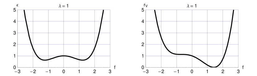
Figure 1: Vacuum energy densities $\epsilon(f)$ [on the left] and $r_{V}(f)$ [on the right] for nonzero cosmological constant $\lambda=1$. The relevant expression for these vacuum energy densities are given by (10) and (13), with the constant (12b). The vacuum energy density $r_{V}(f)$ is the quantity that gravitates.

III Bubble without gravity

III.1 Preliminaries

It is relatively easy to get a result for a special case. First, we set

$$G=0\,,$$ (18)

so that we just have Minkowski spacetime to consider.

Second, we recall from Sec. II that the generalized Maxwell equation KV2008a ; KV2008b gives rise to the nonlinear-Klein–Gordon equation (6), which reads explicitly

$$\Box\,q=q_{0}\,\frac{d\rho_{V}}{dq}\,,$$ (19)

with the flat-spacetime d’Alembertian $\Box\equiv\eta^{\alpha\beta}\,\partial_{\alpha}\partial_{\beta}=-\partial_{t}^{2}+\nabla^{2}$.

Third, introducing spherical coordinates, the $q$-field of a spherical bubble is given by

$$q=q(t,\,r)\,.$$ (20)

Fourth, we start from a bubble with essentially $q_{\text{inside}}=\widehat{q}\neq q_{0}$ and $q_{\text{outside}}=q_{0}$. Outside the bubble, the $q$-field has already compensated the initial cosmological constant $\Lambda\geq 0$ (the case of an arbitrary-sign initial cosmological constant $\Lambda$ has been considered in Ref. KV2016-Lambda-cancellation ). The question, now, is how the inside $q$-field evolves with time.

III.2 Numerics

The numerical solution will be obtained by use of the dimensionless variables introduced in Sec. II. The partial differential equation (PDE) from (19) for the spherically symmetric $q$-field (20) then reads

$$\partial_{\tau}^{2}\,f(\tau,\,\rho)-\frac{1}{\rho^{2}}\,\partial_{\rho}\left[\rho^{2}\,\partial_{\rho}\,f(\tau,\,\rho)\right]=-\left[\frac{d}{df}\,r_{V}(f)\right]_{f=f(\tau,\,\rho)}\,,$$ (21)

where $r_{V}(f)$ is given by (13) with (10) and (12b). The initial values at $\tau=0$ and the boundary conditions at $\rho=0$ and $\rho=\infty$ are

$$f(0,\,\rho) = f_{\text{start}}(\rho)\,,$$ (22a)

$$\partial_{\tau}f(0,\,\rho) = 0\,,$$ (22b)

$$\partial_{\rho}\,f(\tau,\,0) = 0\,,$$ (22c)

$$f(\tau,\,\infty) = f_{0}\,.$$ (22d)

Practically, we restrict the $\rho$ range to $\{\rho_{\text{min}},\rho_{\text{max}}\}$ with $\rho_{\text{min}}\geq 0$ and $\rho_{\text{max}}<\infty$. Also, we use the following explicit start function:

$$f_{\text{start}}(\rho) = \left\{\begin{array}[]{cl}\widehat{f}\,,&\;\;\text{for}\;\;\rho\in(0,\,\overline{\rho}-1/2)\,,\\[2.84526pt] \widehat{f}+\sin^{4}\Big{[}\big{(}\rho-\overline{\rho}+1/2\big{)}\pi/2\Big{]}\,\big{(}f_{0}-\widehat{f}\big{)}\,,&\;\;\text{for}\;\;\rho\in[\overline{\rho}-1/2,\,\overline{\rho}+1/2]\,,\\[2.84526pt] f_{0}\,,&\;\;\text{for}\;\;\rho\in(\overline{\rho}+1/2,\infty)\,,\end{array}\right.$$ (23d)

where, for now, we set $$\overline{\rho}=1$$ and take

$$\widehat{f} = 0\,.$$ (23e)

Note that the fourth power of the sine-function in (23) makes for a continuous second-order derivative at $\rho=\overline{\rho}\pm 1/2$.

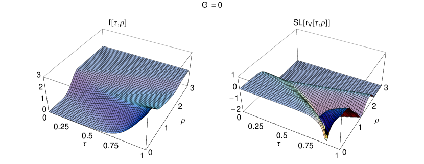
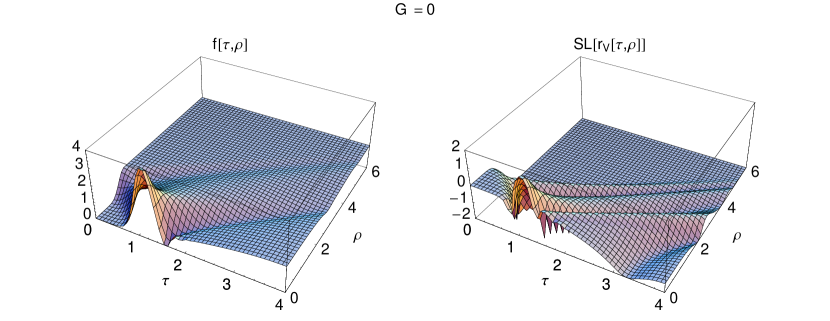
Figure 2: Numerical solution of the flat-spacetime PDE (21) for the case of a nonzero cosmological constant, $\lambda=1$. The initial values are (22a) from the start function (23) with $\overline{\rho}=1$ and (22b). The boundary conditions are (22c) at $\rho_{\text{min}}=0$ and (22d) at $\rho_{\text{max}}=4$. The $f(\tau,\,\rho)$ field is calculated over a relatively short time interval, $\tau\in[0,\,1]$. Also plotted is the corresponding energy density $r_{V}$, using the shift-log function defined by $\text{SL}(x)\equiv\log_{10}(x+0.01)\in[-2,\,\infty)$ for $x\geq 0$. This vacuum energy density $r_{V}[f]$ for $\lambda=1$ is given by (13) with (10) and (12b). The vacuum energy density $r_{V}[f]$ is, in fact, the quantity that would gravitate if $G$ were nonzero.

Figure 3: Same as Fig. 3, but now evolved over a larger time interval, $\tau\in[0,\,4]$.

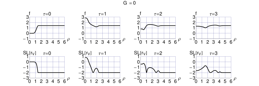
Figure 4: Four time-slices from the numerical solution of Fig. 3.

The general behavior of the numerical solution is displayed in Figs. 3 and 3 and four time-slices are given in Fig. 4. These results show the disappearance of the bubble “domain-wall” and the start of the outward motion of its remnant. Observe, in Fig. 3, both spatial $r_{V}$ oscillations (for example, at $\tau=4$) and temporal $r_{V}$ oscillations (for example, at $\rho=0$). The temporal $r_{V}$ oscillations were first observed for a homogeneous context in Ref. KV2008b , but new here is that energy can escape towards the surrounding unperturbed space.

These numerical results demonstrate that the out-moving $r_{V}$ disturbance has a rapidly decreasing amplitude. Incidentally, the quality of the numerical solution can be monitored by evaluating the numerical value of the integral of motion (energy) corresponding to the field equation (21); see also Sec. IV.2.

III.3 Discussion

The numerical results of Sec. III.2 show two characteristics of the $q$-bubble time evolution in the absence of gravitational effects:

1. initially, the bubble wall gives rise to both out-moving and in-moving disturbances of the dimensionless vacuum energy density $r_{V}$, where the in-moving disturbance makes for an increased energy density at the center;

2. ultimately, there is an out-moving $r_{V}$ disturbance with a rapidly diminishing amplitude (asymptotically, $r_{V}\sim 1/\rho^{2}\sim 1/\tau^{2}$ from energy conservation).

Even for the simple case of zero gravity, this makes the numerical calculation of large bubbles difficult. There are, then, two very different scales, namely the bubble radius ($\overline{\rho}\gg 1$) and the width of the bubble wall ($\Delta\rho\sim 1$).

Remark, finally, that the above two characteristics of the $q$-bubble dynamics are very different from those of Coleman’s vacuum bubble, as mentioned already in Sec. I. Indeed, Coleman’s vacuum bubble Coleman1977 has no in-moving disturbance and an essentially constant domain-wall profile in its rest-frame, energy being supplied by the “false” vacuum.

IV Bubble with gravity

IV.1 Preliminaries and Ansätze

From now on, we set

$$G=G_{N}\,,$$ (24)

where $G_{N}$ is Newton’s gravitational coupling constant Tanabashi-etal2018 .

The spherically symmetric Ansatz for the metric in Kodama–Schwarzschild coordinates $(t,\,r,\,\theta,\,\phi)$ reads AbreuVisser2010

$$g_{\alpha\beta}=\left[\text{diag}\left(-e^{-2\Phi(t,\,r)}\,\left[1-\frac{2\,G_{N}\,m(t,\,r)}{r}\right],\,\left[1-\frac{2\,G_{N}\,m(t,\,r)}{r}\right]^{-1},\,r^{2},\,r^{2}\,\sin^{2}\theta\right)\right]_{\alpha\beta}\,,$$ (25)

and the spherically symmetric Ansatz for the matter field is simply

$$q=q(t,\,r)\,.$$ (26)

It is a straightforward exercise to insert these Ansätze into the field equations (6) and (8) from the action (1). In this way, the reduced nonlinear-Klein–Gordon equation and the reduced Einstein equations are obtained (these expressions will be given in Sec. IV.2).

IV.2 Dimensionless PDEs

As mentioned in Sec. II, specifically in the paragraph above (10), we make all variables dimensionless by use of $q_{0}>0$, which we now take to have the following numerical value:

$$q_{0}\equiv g\,(G)^{-1}=g\,(G_{N})^{-1}\equiv g\,(E_{\text{Planck}})^{2}\approx g\,\left(1.22\times 10^{19}\,\text{GeV}\right)^{2}\,.$$ (27)

With $q_{0}\equiv(E_{\text{$q$-field}})^{2}$, the number $g$ here can be interpreted as a hierarchy factor,

$$g=\left(E_{\text{$q$-field}}/E_{\text{Planck}}\right)^{2}\,.$$ (28)

Added to our previous dimensionless $q$-field Ansatz function $f(\tau,\,\rho)$, we now have two dimensionless metric Ansatz functions, making for a total of three Ansatz functions:

$$\Big{\{}f(\tau,\,\rho)\,,\Phi(\tau,\,\rho)\,,\mu(\tau,\,\rho)\Big{\}}\,.$$ (29)

A useful definition is

$$B(\tau,\,\rho)\equiv 1-2\,\mu(\tau,\,\rho)/\rho\,,$$ (30)

as precisely this combination enters the metric Ansatz (25) by the square bracket factors in $g_{\tau\tau}$ and $g_{\rho\rho}$, using dimensionless coordinates $\tau$ and $\rho$ instead of $t$ and $r$.

The reduced nonlinear-Klein–Gordon equation corresponds to the following PDE:

$$\frac{e^{2\Phi}}{B}\,\ddot{f}-B\,\frac{1}{\rho^{2}}\,\partial_{\rho}\Big{(}\rho^{2}\,f^{\prime}\Big{)}+\frac{e^{2\Phi}}{B}\,\left(\dot{\Phi}+\frac{2\,\dot{\mu}}{\rho\,B}\right)\,\dot{f}+\left(B\,\Phi^{\prime}+\frac{2\,\mu^{\prime}}{\rho}-\frac{2\,\mu}{\rho^{2}}\right)\,f^{\prime}=-\frac{dr_{V}}{df}\,,$$ (31)

where an overdot stands for differentiation with respect to the dimensionless time coordinate $\tau$ and a prime for differentiation with respect to the dimensionless radial coordinate $\rho$. The reduced Einstein equations give the following first-order PDEs:

$$\frac{\mu^{\prime}}{\rho^{2}} = 4\pi\,g\,\left[r_{V}+B\,\frac{1}{2}\,\big{(}f^{\prime}\big{)}^{2}+\frac{e^{2\Phi}}{B}\,\frac{1}{2}\,\big{(}\dot{f}\big{)}^{2}\right]\,,$$ (32a)

$$\frac{\dot{\mu}}{\rho^{2}\,B} = 4\pi\,g\,f^{\prime}\,\dot{f}\,,$$ (32b)

$$\frac{\Phi^{\prime}}{\rho}\,B = 8\pi\,g\,r_{V}-2\,\mu^{\prime}/\rho^{2}\,,$$ (32c)

and the following second-order PDE:

$$\frac{\mu^{\prime\prime}}{\rho}+\frac{e^{\Phi}}{\rho\,\sqrt{B}}\,\partial_{\rho}\,\Big{[}\rho\,B^{3/2}\,e^{-\Phi}\,\Phi^{\prime}\Big{]}+\frac{e^{\Phi}}{\rho}\,\partial_{\tau}\,\left[\frac{e^{\Phi}}{B^{2}}\,\dot{\mu}\right]=8\pi\,g\,\left\{r_{V}+B\,\frac{1}{2}\,\big{(}f^{\prime}\big{)}^{2}-\frac{e^{2\Phi}}{B}\,\frac{1}{2}\,\big{(}\dot{f}\big{)}^{2}\right\}\,.$$ (33)

Note that we have used (32a) to get the expression on the right-hand side of (32c).

The following consistency check holds: the second-order PDE (33) is solved by the solutions of the first-order PDEs (32) and the second-order PDE (31). It is a well-known fact that the same holds for the reduced ordinary differential equations (ODEs) of the standard Friedmann–Robertson–Walker universe. Specifically, the second-order reduced Einstein ODE follows from the first-order reduced Einstein ODE (a.k.a. the Friedmann equation) by use of the energy-momentum-conservation relations of the perfect fluid considered. Ultimately, this redundancy of the reduced field equations traces back to the invariance of the theory under general coordinate transformations; cf. Sec. 15.1, p. 473 of Ref. Weinberg1972 .

We can also obtain a useful $g$-independent relation from (32a) and (32b) in three steps. First, we extract $\mu^{\prime}$ from (32a) and take the $\tau$ derivative. Second, we extract $\dot{\mu}$ from (32b) and take the $\rho$ derivative, Third, we equate the two expressions for $\dot{\mu}^{\prime}$. The obtained relation is

$$\partial_{\tau}\left(\rho^{2}\left[r_{V}+B\,\frac{1}{2}\,\big{(}f^{\prime}\big{)}^{2}+\frac{e^{2\Phi}}{B}\,\frac{1}{2}\,\big{(}\dot{f}\big{)}^{2}\right]\right)=\partial_{\rho}\,\left(\rho^{2}\,B\,f^{\prime}\,\dot{f}\right)\,,$$ (34)

which may be interpreted as a current-conservation relation. Indeed, for the setup of our initial-value problem (with $f=f_{0}=\text{constant}$ for $\rho\geq\overline{\rho}+1/2$ at $\tau=0$), the integral of (34) gives the following conserved energy $E$:

$$E = \sqrt{q_{0}}\,\int_{0}^{\infty}d\rho\;4\pi\rho^{2}\;e\,,$$ (35a)

$$e = r_{V}+B\,\frac{1}{2}\,\big{(}f^{\prime}\big{)}^{2}+\frac{e^{2\Phi}}{B}\,\frac{1}{2}\,\big{(}\dot{f}\big{)}^{2}\,,$$ (35b)

where the equilibrium value $q_{0}$ of the $q$ variable in the four-form-field-strength realization (1c) has been used to make lengths and times dimensionless (Sec. II). Incidentally, the relation (34) reproduces the reduced nonlinear-Klein–Gordon equation (31) upon use of (32).

Consistent with the expected de-Sitter behavior $m(t,\,r)\propto r^{3}$ near the center and the expected Schwarzschild behavior $m(t,\,r)\sim\text{constant}$ towards spatial infinity, we take the following boundary conditions on the dimensionless metric function $\mu(\tau,\,\rho)$:

$$\mu(\tau,\,0) = 0\,,$$ (36a)

$$\partial_{\rho}\,\mu(\tau,\,\infty) = 0\,.$$ (36b)

For the other metric function $$\Phi(\tau,\,\rho)$$, we take

$$\Phi(\tau,\,0) = 0\,,$$ (36c)

$$\partial_{\rho}\,\Phi(\tau,\,\infty) = 0\,.$$ (36d)

The boundary conditions on $f(\tau,\,\rho)$ have already been given in (22c) and (22d). From the boundary conditions (36), we find that the reduced Einstein equations (32) and (33), for the case $g=0$, give $\mu(\tau,\,\rho)=0$ and $\Phi(\tau,\,\rho)=0$, so that (31) reproduces the flat-spacetime PDE (21).

IV.3 Numerics

IV.3.1 Numerical procedure

Finding the numerical solution of the PDEs (31), (32), and (33) is a nontrivial task. In the following local approach, we are inspired by the discussion of App. A.

The coordinates $\rho$ and $\tau$ are put on a finite grid with $N_{\rho}$ and $N_{\tau}=2\,N_{\rho}$ points, respectively. The PDEs (31), (32c), and (33) are then solved with time-derivatives of $f$ and $\mu$ replaced by forward time-differences and the time-derivative of $\Phi$ replaced by a backward time-difference.

IV.3.2 Numerical solutions

For the presentation of our numerical results, we will employ time-slice plots (cf. Fig. 4) rather than surface plots (cf. Figs. 3 and 3). The various time-slices will be collected in a single plot by color-coding the different time values.

The numerical solution for $g=0$ (Fig. 6) can now be compared with the one for $g=1/400$ (Fig. 6). For the last case, in particular, it has been verified that the numerically obtained functions $f(\tau,\,\rho)$, $\mu(\tau,\,\rho)$, and $\Phi(\tau,\,\rho)$ give residuals of the first-order PDEs (32a) and (32b) that drop to zero as the number of grid points increases.

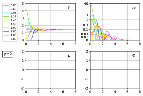
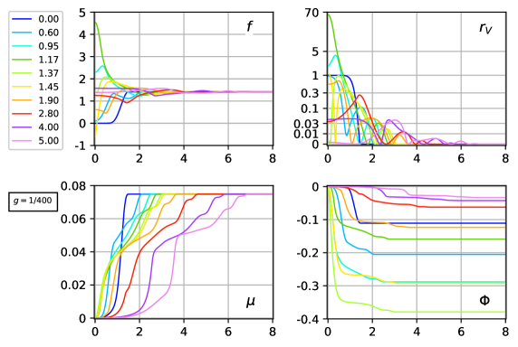
Figure 5: Numerical solution of the PDEs (31), (32), and (33): plots of $f(\tau,\,\rho)$, $r_{V}(\tau,\,\rho)$, $\mu(\tau,\,\rho)$, and $\Phi(\tau,\,\rho)$ at different time slices, with $\tau$ values given in the legend on the left-hand side. The model parameters are $\lambda=1$ and $g=0$. The initial values are: $f(0,\rho)$ as given by (23) with $\overline{\rho}=1$ and $\dot{f}(0,\rho)=0$. The metric functions $\mu(\tau,\,\rho)$ and $\Phi(\tau,\,\rho)$ vanish identically. The vacuum energy density $r_{V}$ is plotted as $\log_{10}(r_{V}+0.01)$.

Figure 6: Same as Fig. 6, again with $\lambda=1$ but now for $g=0.0025$. The initial values are: $f(0,\rho)$ as given by (23) with $\overline{\rho}=1$, $\dot{f}(0,\rho)=0$, $\mu(0,\rho)$ from (32a), and $\Phi(0,\rho)$ from (32c).

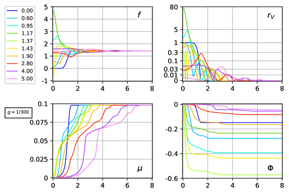
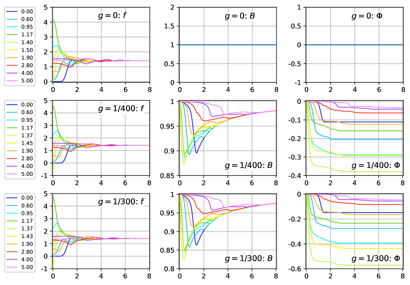
Figure 7: Same as Fig. 6, but now for $g=0.0033\!\!\not{\!3}$.

Figure 8: Comparison of the numerical solutions from Figs. 6–8, showing, in particular, the behavior of the quantity $B$ from (30), which enters the metric (25). The various time-slices at the three different values of $g$ are given by the respective legends on the left.

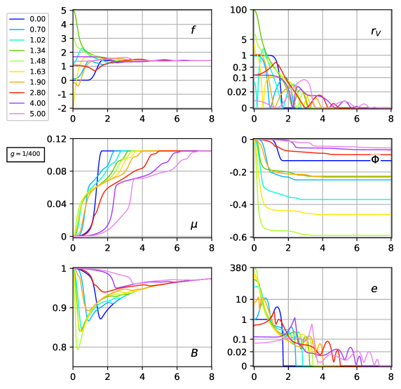
Figure 9: Same as Fig. 6, but now with $\overline{\rho}=1.2$ instead of $\overline{\rho}=1$. Two additional panels show the metric quantity $B(\tau,\,\rho)$ from (30) and the energy density $e(\tau,\,\rho)$ from (35b). The energy densities $e$ and $r_{V}$ are plotted using the same scale function $\log_{10}(x+0.005)$ but with different over-all factors. The $r_{V}$ peak at $(\tau,\,\rho)\sim(1.34,\,0)$ of the $\overline{\rho}=1.2$ solution is significantly larger than the corresponding peak of the $\overline{\rho}=1$ solution in Fig. 6. Similarly, the $B$ dip of the $\overline{\rho}=1.2$ solution is significantly lower than the corresponding dip of the $\overline{\rho}=1$ solution in the $B$ panel of the middle row of Fig. 8.

For somewhat larger $g$ values, a Schwarzschild-type horizon is formed, as the energy density $e$ becomes large close to the center $\rho=0$. This horizon is apparently different from a de-Sitter-type horizon which arises from a constant vacuum energy density far away from the center; see App. B for a brief discussion of the de-Sitter-type spacetime near the $q$-bubble origin. With the setup and boundary conditions from Fig. 6, we estimate horizon formation to occur for $g\gtrsim 0.006$. The regular numerical solution at $g=1/300$ is shown in Fig. 8. The evolution towards the formation of a horizon, with $B(\tau,\,\rho)$ from (30) dipping to zero, is illustrated in Fig. 8.

For a large bubble, we expect that, from the ingoing $r_{V}$ disturbance (cf. Figs. 3 and 3), the $r_{V}$ peak close to the origin will be higher than the one for a small bubble. This behavior is confirmed by comparing Fig. 9 with Fig. 6. The $f$-panel in Fig. 9 also shows that the quantities $(\dot{f})^{2}$ and $(f^{\prime})^{2}$ are large at $(\tau,\,\rho)\sim(1.5,\,0)$, with both terms contributing significantly to the energy density $e$ close to the center $\rho=0$.

IV.4 Discussion

The numerical results of Sec. IV.3.2 show that the vacuum energy density of a nonequilibrium $q$-bubble embedded in the equilibrium vacuum with $q=q_{0}=\text{constant}$ evolves in a complicated way. For a sufficiently small $q$-bubble, part of the vacuum energy density $r_{V}$ of the bubble wall, first, moves inwards towards the center and, then, rapidly disperses (cf. Figs. 3 and 3).

The numerical calculations were performed for the case with gravity turned off ($G=0$) and turned on ($G>0$). Qualitatively, the main effect of gravity is to give a larger maximum value of the vacuum energy density at the center $\rho=0$ (compare the $r_{V}$ panels of Fig. 6 and 6).

If the hierarchy ratio $g$ from (28) is approximately equal to or somewhat above $0.006$, the particular solution develops a Schwarzschild-type horizon near the center $\rho=0$ and different coordinates need to be chosen (cf. App. B). We postpone this analysis to a future publication, as the focus of the present article is on the dispersion of vacuum energy if the Big Bang occurs in a finite region of space surrounded by equilibrium vacuum (where any form of initial vacuum energy has already been cancelled KV2008a ; KV2008b ; KV2016-Lambda-cancellation ).

V Conclusions

In the present article, we have obtained a first glimpse of the inhomogeneous dynamics of the gravitating vacuum energy density $\rho_{V}(q)$ as described by the vacuum variable $q$ originating from a four-form field strength (earlier work KV2008b ; KV2016-Lambda-cancellation considered the time-evolution of spatially-constant $q$-fields). In this new probe of $q$-theory, we start from a large vacuum energy density in a finite region of space surrounded by equilibrium vacuum, and follow the time evolution of the vacuum energy density.

Our numerical results show the possibility of obtaining different evolution scenarios depending on the initial conditions and the parameters of the vacuum energy. These results suggest that there may be de-Sitter expansion within a finite region of space, gravitational collapse of the vacuum medium with the formation of a singularity, and formation of cosmological and/or black-hole horizons.

It may also be of interest to study the vacuum structure at the black hole singularity. The singularity may be smoothened, as the gravitational coupling depends, in general, on the value of the $q$ variable and gravity may be effectively turned off near the center. We leave this study to a future investigation.

Appendix A Integro-differential equations

The role of $\Phi(\tau,\,\rho)$ in the PDEs (31), (32), and (33) is rather subtle. From (32c), we have

$$\Phi^{\prime}=\frac{8\pi\,g\,\rho\,r_{V}-2\,\mu^{\prime}/\rho}{1-2\,\mu/\rho}\,,$$ (37)

which can be integrated to give

$$\widehat{\Phi}(\tau,\,\rho)=\int_{0}^{\rho}\,d\widetilde{\rho}\;\frac{8\pi\,g\,\widetilde{\rho}\,r_{V}[f(\tau,\,\widetilde{\rho})]-2\,\mu^{\prime}(\tau,\,\widetilde{\rho})/\widetilde{\rho}}{1-2\,\mu(\tau,\,\widetilde{\rho})/\widetilde{\rho}}\,,$$ (38)

where the prime in the numerator of the integrand stands for differentiation with respect to $\widetilde{\rho}$. Hence, $\widehat{\Phi}(\tau,\,\rho)$ is determined nonlocally by the functions $f(\tau,\,\widetilde{\rho})$ and $\mu(\tau,\,\widetilde{\rho})$ at the same time slice $\tau$.

The PDEs (31) and (33) still involve $\Phi$ and its time-derivative $\dot{\Phi}$ [the spatial derivatives $\Phi^{\prime}$ and $\Phi^{\prime\prime}$ can be eliminated by use of (32c)]. Replacing $\Phi(\tau,\,\rho)$ by $\widehat{\Phi}(\tau,\,\rho)$ from (38), these two equations become integro-differential equations solely involving the functions $f(\tau,\,\rho)$ and $\mu(\tau,\,\rho)$. Explicitly, these equations read:

$$\frac{e^{2\widehat{\Phi}}}{B}\,\ddot{f}-B\,\frac{1}{\rho^{2}}\,\partial_{\rho}\Big{(}\rho^{2}\,f^{\prime}\Big{)}+\frac{e^{2\widehat{\Phi}}}{B}\,\left(\partial_{\tau}\widehat{\Phi}+\frac{2\,\dot{\mu}}{\rho\,B}\right)\,\dot{f}+\left(B\,\widehat{\Phi}^{\prime}+\frac{2\,\mu^{\prime}}{\rho}-\frac{2\,\mu}{\rho^{2}}\right)\,f^{\prime}=-\frac{dr_{V}}{df}\,,$$ (39a)

$$\frac{\mu^{\prime\prime}}{\rho}+\frac{e^{\widehat{\Phi}}}{\rho\,\sqrt{B}}\,\partial_{\rho}\Big{[}\rho\,B^{3/2}\,e^{-\widehat{\Phi}}\,\widehat{\Phi}^{\prime}\Big{]}+\frac{e^{\widehat{\Phi}}}{\rho}\partial_{\tau}\left[\frac{e^{\widehat{\Phi}}}{B^{2}}\,\dot{\mu}\right]=8\pi\,g\left\{r_{V}+B\,\frac{1}{2}\,\big{(}f^{\prime}\big{)}^{2}-\frac{e^{2\widehat{\Phi}}}{B}\,\frac{1}{2}\,\big{(}\dot{f}\big{)}^{2}\right\},$$ (39b)

with $\widehat{\Phi}$ given by the expression (38) and $\partial_{\tau}\widehat{\Phi}$ having the $\tau$-derivative pulled inside the $\widetilde{\rho}$ integral.

Appendix B Bubble interior

The $q$-bubble setup considered in this article has a start configuration $f(0,\,\rho)$ determined by (23) and the further initial condition $\dot{f}(0,\,\rho)=0$. Then, the reduced field equation (32a) gives that the metric Ansatz function $\mu(\tau,\,\rho)$ behaves near the center as $\mu(\tau,\,\rho)\propto\rho^{3}$. This behavior of $\mu$ allows for the following definition of the quantity $h(\tau)$:

$$\lim_{\rho\to 0}\frac{2\,\mu(\tau,\,\rho)}{\rho^{3}} \equiv h^{2}(\tau).$$ (4)

Near the spacetime origin ($\rho=\tau=0$) of the $q$-bubble considered, we have

$$h^{2}(\tau) \sim h^{2}(0)\equiv h_{0}^{2}\,,$$ (5a)

$$\Phi(0,\,0) \sim 0\,,$$ (5b)

$$r_{V}(0,\,0) \sim r_{V0}>0\,,$$ (5c)

with constants $r_{V0}$ and $h_{0}$. In fact, the reduced field equation (32a) gives

$$h_{0}^{2}=(8\pi/3)\,g\,r_{V0}\,,$$ (6)

where $g$ has been defined in (27). The resemblance of (6) with the spatially flat Friedmann equation Weinberg1972 of a universe with constant vacuum energy will become clear later on.

Writing the metric (25) in terms of dimensionless variables gives

$$ds^{2} = -e^{-2\Phi(\tau,\,\rho)}\,\left[1-\frac{2\,\mu(\tau,\,\rho)}{\rho}\right]\,d\tau^{2}+\left[1-\frac{2\,\mu(\tau,\,\rho)}{\rho}\right]^{-1}\,d\rho^{2}$$ (7)

$$+\rho^{2}\Big{(}d\theta^{2}+\sin^{2}\theta\,d\phi^{2}\Big{)}\,.$$

With the behavior (4) and (5), the metric (7) near the spacetime origin of the $q$-bubble ($\rho=\tau=0$) becomes

$$ds^{2}\,\Big{|}_{\text{origin}} \sim -\Big{[}1-h_{0}^{2}\,\rho^{2}\Big{]}\,d\tau^{2}+\Big{[}1-h_{0}^{2}\,\rho^{2}\Big{]}^{-1}\,d\rho^{2}+\rho^{2}\Big{(}d\theta^{2}+\sin^{2}\theta\,d\phi^{2}\Big{)}\,,$$ (8)

which corresponds to the metric of de-Sitter spacetime in so-called static coordinates Schroedinger1956 ; HawkingEllis1973 ; BirrellDavies1982 . Note that, if $\rho$ were allowed to be large enough, the metric on the right-hand side of (8) would display a coordinate singularity at $\rho=1/h_{0}$.

Now, introduce new dimensionless coordinates (denoted by a hat) from the following relations:

$$\exp(h_{0}\,\widehat{\tau}) = \sqrt{(1-h_{0}^{2}\,\rho^{2})}\,\Big{[}\cosh(h_{0}\,\tau)+\sinh(h_{0}\,\tau)\Big{]}\,,$$ (9a)

$$h_{0}\,\widehat{z} = \frac{h_{0}\,\rho\,\cos\theta}{\sqrt{(1-h_{0}^{2}\,\rho^{2})}\,\Big{[}\cosh(h_{0}\,\tau)+\sinh(h_{0}\,\tau)\Big{]}}\,,$$ (9b)

$$h_{0}\,\widehat{y} = \frac{h_{0}\,\rho\,\sin\theta\,\cos{\phi}}{\sqrt{(1-h_{0}^{2}\,\rho^{2})}\,\Big{[}\cosh(h_{0}\,\tau)+\sinh(h_{0}\,\tau)\Big{]}}\,,$$ (9c)

$$h_{0}\,\widehat{x} = \frac{h_{0}\,\rho\,\sin\theta\,\sin{\phi}}{\sqrt{(1-h_{0}^{2}\,\rho^{2})}\,\Big{[}\cosh(h_{0}\,\tau)+\sinh(h_{0}\,\tau)\Big{]}}\,.$$ (9d)

With these new coordinates, the metric (8) near the spacetime origin of the $q$-bubble ($\widehat{\tau}=\widehat{z}=\widehat{y}=\widehat{x}=0$) becomes

$$ds^{2}\Big{|}_{\text{origin}} \sim -(d\widehat{\tau})^{2}+\big{[}a(\widehat{\tau})\big{]}^{2}\,\Big{[}(d\widehat{x})^{2}+(d\widehat{y})^{2}+(d\widehat{z})^{2}\Big{]}\,,$$ (10a)

$$a(\widehat{\tau}) \equiv \exp(h_{0}\,\widehat{\tau})\,.$$ (10b)

Note that the spatially-flat Robertson–Walker metric on the right-hand side of (10a) with the scale factor (10b) no longer has the nontrivial coordinate singularity. From the scale factor $a(\widehat{\tau})$ in (10b), we obtain $(da/d\widehat{\tau})/a=h_{0}$, so that the quantity $h_{0}$, which was originally defined by (4) and (5), can be interpreted as a Hubble constant. The scale factor $a(\widehat{\tau})$ of (10) displays, for $h_{0}\,\widehat{\tau}\gg 1$, the well-known exponential expansion of de-Sitter spacetime Schroedinger1956 ; HawkingEllis1973 ; BirrellDavies1982 .

The numerical solution of Fig. 6, however, has $h_{0}\approx 0.14$ for $\tau\lesssim 0.4$ and does not show the exponential expansion. Needed is an initial bubble (23) with $\overline{\rho}\gg 1$ (the required order of magnitude for $\overline{\rho}$ is $1/h_{0}\sim 1/\sqrt{g\,r_{V0}}\,$). But there are three problems with such large bubbles. First, as noted in Sec. III.3, the numerics of a large $q$-bubble is challenging.

Second, the coordinate singularity of (8) at $\rho=1/h_{0}$ suggests that the metric Ansatz (7) is inappropriate. Most likely, this problem can be evaded by use of another metric Ansatz, possibly inspired by Painlevé–Gullstrand coordinates Painleve1921 ; Gullstrand1922 ; MartelPoisson2000 ; Volovik2009 .

Third, large bubbles may give gravitational collapse close to the center $\rho=0$, as the energy density $e$ from (35b) becomes large at the center. See Fig. 3, where the initial ($\tau\sim 0$) bubble-wall disturbance of the vacuum energy density $r_{V}$ separates around $\tau\sim 0.3$ into an outgoing and ingoing disturbance, the latter giving a peak of $r_{V}$ at $\rho=0$ for $\tau\sim 1$. See also Fig. 9, which shows that the numerical solution with a somewhat larger value of $\overline{\rho}$ has a significantly larger $r_{V}$ peak at the origin than the numerical solution of Fig. 6.

References

- (1) Ya.B. Zel’dovich, “The cosmological constant and the theory of elementary particles,” Sov. Phys. Usp. 11, 381 (1968).
- (2) S. Weinberg, “The cosmological constant problem,” Rev. Mod. Phys. 61, 1 (1989).
- (3) M. Tanabashi et al. [Particle Data Group], “Review of Particle Physics,” Phys. Rev. D 98, 030001 (2018).
- (4) S.W. Hawking, “The cosmological constant is probably zero,” Phys. Lett. B 134, 403 (1984).
- (5) F.R. Klinkhamer and G.E. Volovik, “Self-tuning vacuum variable and cosmological constant,” Phys. Rev. D 77, 085015 (2008), arXiv:0711.3170.
- (6) F.R. Klinkhamer and G.E. Volovik, “Dynamic vacuum variable and equilibrium approach in cosmology,” Phys. Rev. D 78, 063528 (2008), arXiv:0806.2805.
- (7) F.R. Klinkhamer and G.E. Volovik, “Dynamic cancellation of a cosmological constant and approach to the Minkowski vacuum,” Mod. Phys. Lett. A 31, 1650160 (2016), arXiv:1601.00601.
- (8) F.R. Klinkhamer and G.E. Volovik, “Brane realization of -theory and the cosmological constant problem,” JETP Lett. 103, 627 (2016), arXiv:1604.06060.
- (9) F.R. Klinkhamer and G.E. Volovik, “Tetrads and -theory,” JETP Lett. 109, 364 (2019), arXiv:1812.07046.
- (10) F.R. Klinkhamer and G.E. Volovik, “Dynamics of the quantum vacuum: Cosmology as relaxation to the equilibrium state,” J. Phys. Conf. Ser. 314, 012004 (2011), arXiv:1102.3152.
- (11) T. Markkanen, “De Sitter stability and coarse graining,” Eur. Phys. J. C 78, 97 (2018), arXiv:1703.06898.
- (12) H. Matsui, “Instability of de Sitter spacetime induced by quantum conformal anomaly,” JCAP 1901, 003 (2019), arXiv:1806.10339.
- (13) V.M.H. Ruutu et al., “Vortex formation in neutron-irradiated superfluid 3He as an analogue of cosmological defect formation,” Nature 382, 334 (1996).
- (14) S R. Coleman, “The fate of the false vacuum. 1. Semiclassical theory,” Phys. Rev. D 15, 2929 (1977); Erratum: Phys. Rev. D 16, 1248 (1977).
- (15) C.G. Callan, Jr. and S.R. Coleman, “The fate of the false vacuum. 2. First quantum corrections,” Phys. Rev. D 16, 1762 (1977).
- (16) S.R. Coleman and F. De Luccia, “Gravitational effects on and of vacuum decay,” Phys. Rev. D 21, 3305 (1980).
- (17) M.W. Choptuik, “Universality and scaling in gravitational collapse of a massless scalar field,” Phys. Rev. Lett. 70, 9 (1993).
- (18) R.L. Marsa and M.W. Choptuik, “Black-hole–scalar-field interactions in spherical symmetry,” Phys. Rev. D 54, 4929 (1996), arXiv:gr-qc/9607034.
- (19) E.P. Honda and M.W. Choptuik, “Fine structure of oscillons in the spherically symmetric Klein-Gordon model,” Phys. Rev. D 65, 084037 (2002), arXiv:hep-ph/0110065.
- (20) M.W. Choptuik, L. Lehner, and F. Pretorius, “Probing strong field gravity through numerical simulations,” arXiv:1502.06853.
- (21) V. Cardoso, L. Gualtieri, C. Herdeiro, and U. Sperhake, “Exploring new physics frontiers through numerical relativity,” Living Rev. Relativity 18, 1 (2015), arXiv:1409.0014.
- (22) F.R. Klinkhamer and G.E. Volovik, “Propagating -field and -ball solution,” Mod. Phys. Lett. A 32, 1750103 (2017), arXiv:1609.03533.
- (23) F.R. Klinkhamer and G.E. Volovik, “Dark matter from dark energy in -theory,” JETP Lett. 105, 74 (2017), arXiv:1612.02326.
- (24) F.R. Klinkhamer and G.E. Volovik, “More on cold dark matter from -theory,” arXiv:1612.04235.
- (25) F.R. Klinkhamer and T. Mistele, “Classical stability of higher-derivative -theory in the four-form-field-strength realization,” Int. J. Mod. Phys. A 32, 1750090 (2017), arXiv:1704.05436.
- (26) S. Weinberg, Gravitation and Cosmology : Principles and Applications of the General Theory of Relativity (John Wiley and Sons, New York, 1972).
- (27) G. Abreu and M. Visser, “Kodama time: Geometrically preferred foliations of spherically symmetric spacetimes,” Phys. Rev. D 82, 044027 (2010), arXiv:1004.1456.
- (28) E. Schrödinger, Expanding Universes (Cambridge University Press, Cambridge, England, 1956).
- (29) S.W. Hawking and G.F.R. Ellis, The Large Scale Structure of Space-Time (Cambridge University Press, Cambridge, England, 1973).
- (30) N.D. Birrell and P.C.W. Davies, Quantum Fields in Curved Space (Cambridge University Press, Cambridge, England, 1982).
- (31) P. Painlevé, “La mécanique classique et la théorie de la relativité,” C. R. Acad. Sci. (Paris) 173, 677 (1921).
- (32) A. Gullstrand, “Allgemeine Lösung des statischen Einkörper-problems in der Einsteinschen Gravitationstheorie,” Arkiv. Mat. Astron. Fys. 16, 1 (1922).
- (33) K. Martel and E. Poisson, “Regular coordinate systems for Schwarzschild and other spherical space-times,” Am. J. Phys. 69, 476 (2001), arXiv:gr-qc/0001069.
- (34) G.E. Volovik, “Particle decay in de Sitter spacetime via quantum tunneling,” JETP Lett. 90, 1 (2009), arXiv:0905.4639.