TOTEM data and the real part of the hadron elastic amplitude
at 13 TeV

Abstract

We analyse the 13 TeV TOTEM data on elastic proton-proton scattering through a thorough statistical analysis, and obtain that $\rho=0.096\pm 0.006$ and $\sigma_{tot}=(107.5\pm 1.5)$ mb. Theoretical errors could lower the cross section by about 2 mb and increase $\rho$ by about 0.002. We also show that these results do not imply the existence of an odderon at $t=0$.

1 Introduction

The TOTEM collaboration has recently measured [1, 2] with great precision the hadron scattering amplitude in the very forward, low-$t$, region at an energy $\sqrt{s}=13$ TeV. These data show some tension with the best fit of the COMPETE collaboration [3] and this has lead to the claim that the odderon [4] has been discovered at zero momentum transfer, $t=0$ [2, 5, 6]. As the odderon has probably been seen at non-zero $t$ at the ISR [7], this would solve one of the puzzles of hadronic physics, as so far no trace of it has been found at $t=0$. It is thus important to independently check the analysis of Ref. [2].

Before doing this, we want to note that the central value of the COMPETE fits (which agrees with the TOTEM cross section measurements) has no special significance. COMPETE evaluated the systematic error and produced a band of possibilities for models without odderon exchange. The actual predictions, for $\sqrt{s}=13$ TeV, were 86 mb $\leq\sigma_{tot}\leq$ 117 mb for the total cross section and 0.058$\leq\rho(t=0)\leq$0.145 for the ratio of the real part of the amplitude to its imaginary part. This shows that the LHC data do constrain the fits, and that the best fit of 16 years ago is no longer favoured. This does not mean that no fit can accommodate the new data without an odderon.

This letter will first describe the theoretical ingredients used in the present analysis, and show our best fit. We shall then explain what the allowed ranges of forward hadronic observables are in the light of [2]. We shall also note the importance of the data of [1], and stress the role of the normalisation factor in the data.

2 Theory

At extremely small values of $|t|$, the proton-proton elastic cross section is described by Rutherford scattering, i.e. the QED amplitude. At values of $|t|$ larger than 0.01 GeV², it is dominated by the purely hadronic amplitude, which comes from pomeron (and maybe odderon) exchange(s) at high energy. In between, both amplitudes matter, and the phase of the hadronic amplitude can be deduced from the interference between the photon-exchange amplitude and the pomeron-exchange amplitude.

Hence one needs to calculate the interference between the known amplitude due to photon exchange and an unknown one due to pomeron exchange(s). The differential elastic cross section is described by the square of the elastic scattering amplitude ${\cal A}(s,t)$ divided by $s$.

The complete amplitude includes the electromagnetic (Coulomb) and hadronic (Nuclear) interactions and can be expressed as

$${\cal A}(s,t)={\cal A}_{C}(s,t)\exp{(i\alpha\varphi(s,t))}+{\cal A}_{N}(s,t).$$ (1)

The Coulomb amplitude can be conveniently split into several non-interfering parts, according to the helicities of the initial and of the final states. In the one-photon-exchange approximation, one gets five independent amplitudes, which must be summed to obtain ${\cal A}_{C}$ [8, 9]:

$${\cal A}_{C}^{++\to++}(s,t) = {\cal A}_{C}^{+-\to+-}(s,t)=\frac{s\alpha}{t}\ F_{1}^{2}(t)^{2},$$

$${\cal A}_{C}^{++\to--}(s,t) = -{\cal A}_{C}^{+-\to-+}(s,t)=s\alpha\ F_{2}^{2}(t),$$

$${\cal A}_{C}^{++\to+-}(s,t) = -\frac{s\alpha}{\sqrt{|t|}}\ F_{1}(t)\ F_{2}(t),$$ (2)

with the Dirac, Pauli and dipole form factors given by

$$F_{1}(t) = \frac{4\ m_{p}^{2}-\mu_{p}\ t}{4\ m_{p}^{2}-t}\ G_{D},$$

$$F_{2}(t) = \frac{4\ m_{p}^{2}\ (\mu_{p}-1)}{4\ m_{p}^{2}-t}\ G_{D},$$

$$G_{D}(t) = \frac{1}{(1-t/0.71)^{2}},\ \ \$$

and where $\mu_{p}$ is the magnetic moment of the proton and $m_{p}$ its mass.

The phase $\varphi(s,t)$ has been calculated and discussed by many authors. For high energies the first results were obtained by A.I. Akhiezer and I.Ya. Pomeranchuk [10] for the diffraction on a black nucleus. Using the WKB approximation in potential theory, H. Bethe [11] derived it for proton-nucleus scattering and obtained

$$\varphi=2\ln{\left({1.06\over a\sqrt{-t}}\right)},$$ (4)

where the parameter $a$ characterizes the range of the strong-interaction forces and was taken as the size of a nucleus.

After some improvements [12, 13], the most important result was obtained by M.P. Locher [14] and then by B. West and D.R. Yennie [15]. Through the calculation of the associated Feynman diagrams, they obtained a general expression for $\varphi_{CN}(s,t)$ in the case of point-like particles in terms of the hadron elastic scattering amplitude

$$\varphi(s,t)=\log\left({s\over|t|}\right)-\int^{0}_{-s}\frac{dt^{{}^{\prime}}}{|t-t^{{}^{\prime}}|}\ \ \left(1-\frac{{\cal A}_{N}(s,t^{{}^{\prime}})}{{\cal A}_{N}(s,t)}\right).$$ (5)

For an exponential $t$ dependence of the hadron amplitude ${\cal A}_{N}=hs\ \exp\left({B(s)t\over 2}\right)$, we can get

$$\varphi(s,t)=\mp\left[\log\left({B(s)|t|\over 2}\right)+\gamma\right],$$ (6)

where $\gamma$ is the Euler constant and the upper (lower) sign corresponds to the scattering of particles with the same (opposite) charges. We shall use this result to describe ${\cal A}_{C}$.

For the hadron amplitude near $t=0$ and $\sqrt{s}=13$ TeV, we can use the simplest form

$${\cal A}_{N}(s,t)=s{\sigma_{tot}\over 4\pi}(i+\rho(t))\ \exp\left({B(s)t\over 2}\right).$$ (7)

In our analysis, we follow TOTEM [2] and neglect the $t$-dependence of $\rho$.

The exponential form factor and the constant value of $\rho$ may seem simplistic assumptions, which are motivated only by the rather low number of parameters. Nevertheless, we shall see that they give an excellent description of the data at very small $|t|$, with however slightly different parameters from those of the TOTEM analysis. We shall also explain that the form of the parametrisation matters in a very small interval of $t$, and hence the parameters should be considered as effective ones for those values of $t$. For completeness, we shall discuss the uncertainties associated with these assumptions at the end.

3 TOTEM 13 TeV data

TOTEM has published data for the differential elastic cross section at small $|t|$, from which they derived $\sigma_{tot}=(110.6\pm 3.4)$ mb [1] and $\rho=0.10\pm 0.01$, with a theoretical error of 0.01 [2]. The data have systematic errors dominated by the uncertainty on the normalisation. So, in the following, we shall use the possibility to change the normalisation of the data by a factor $n$, as explained in [2].

We also consider three statistical models, all based on a $\chi^{2}$ statistics. The first one used the simple form

$$\chi^{2}=\sum_{i}{(nd_{i}-\theta(t_{i},\rho,\sigma_{tot},B))^{2}\over\sigma_{i}^{2}},$$ (8)

where $d_{i}$ is the central value of the data in the $i^{th}$ bin, $t_{i}$ is the preferred value of $t$ in the bin $[t_{i}^{min},t_{i}^{max}]$, as given in [2] (note that $|t_{i}|\approx\sqrt{t_{i}^{min}t_{i}^{max}}$), $\theta(t_{i},\rho,\sigma_{tot},B)$ is the 3-parameter theoretical model of $d\sigma/dt$, and $\sigma_{i}$ is the statistical error. The second statistics considered here is

$$\chi^{2}=\sum_{i}{(nd_{i}-\theta(t_{i},\rho,\sigma_{tot},B))^{2}\over\Sigma_{i}^{2}},$$ (9)

where $\Sigma_{i}$ is equal to the sum in quadrature of the statistical and systematic errors. Finally, the TOTEM collaboration has provided the correlation matrix $V$ of the systematic errors. Defining $W_{ij}=V_{ij}+\sigma_{i}\delta_{ij}$, one can write

$$\chi^{2}=\sum_{ij}(nd_{i}-\theta(t_{i},\rho,\sigma_{tot},B))W^{-1}_{ij}(nd_{j}-\theta(t_{j},\rho,\sigma_{tot},B)).$$ (10)

79 points	$\sigma_{tot}$ (mb)	$B$ (GeV-2)	$\rho$	$\chi^{2}$/d.o.f.
statistical	$111.75\pm 0.05$	$20.77\pm 0.03$	$0.083\pm 0.004$	0.89
statistical and systematic	$111.75\pm 0.05$	$20.77\pm 0.03$	$0.084\pm 0.004$	0.80
correlated	$111.75\pm 0.13$	$20.77\pm 0.05$	$0.085\pm 0.005$	0.89

Table 1: Fits to the first 79 data points from TOTEM for $0.0008<|t|<0.07$), for a normalisation $n=1$.

We consider the data at small $|t|$, as they determine the value of $\rho(0)$. Following [2], we fit the first 79 points at $0.0008<|t|<0.07$. We show in Table 1 the results of this fit, for the three statistics considered here. The consideration of correlated errors is close to using only statistical errors. This third statistics reproduces the central values of TOTEM. TOTEM uses a much more complicated form [16] for the phase than Eq. (6), but this agreement shows that the effect of the exact expression of the phase is minimal. The big difference is the size of the error bars, due to the fact that TOTEM in its parameter evaluation allowed a global shift in normalisation of 5.5 %, and incorporated this in the error estimate. This brings us to the central question concerning these data. How well do we know their normalisation? And how should one take this uncertainty into account?

The first thing one can do is repeat the exercise of Table 1, but allow the data to be globally shifted by a factor $n$. As this factor controls the total elastic cross section measured by TOTEM in [1], we use the value $n=1.000\pm 0.055$, which corresponds to their measurement $\sigma_{el}=(31.0\pm 1.8)$ mb, and treat the error as a statistical error. We see in Table 2 that the normalisation factor prefers to be around 0.9, so that the total cross section is correspondingly lowered by about $1\sigma$. This is reminiscent of the situation at lower energies [17], where we also found that the data of TOTEM needed to be lowered by about 10 %.

79 points	$\sigma_{tot}$ (mb)	$B$ (GeV-2)	$\rho$	$n$	$\chi^{2}$/d.o.f
statistical	$107.2\pm 1.9$	$20.81\pm 0.04$	$0.098\pm 0.008$	$0.92\pm 0.03$	0.82
stat. and sys.	$107.2\pm 2.1$	$20.81\pm 0.04$	$0.098\pm 0.008$	$0.92\pm 0.04$	0.75
correlated	$106.4\pm 2.2$	$20.80\pm 0.06$	$0.098\pm 0.008$	$0.91\pm 0.04$	0.81

Table 2: Fits to the first 79 data points from TOTEM for $0.0008<|t|<0.07$.

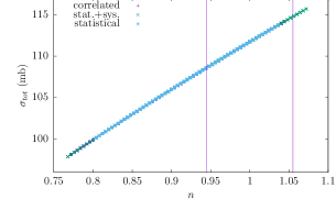
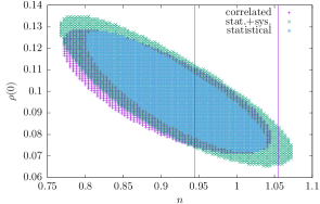
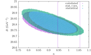
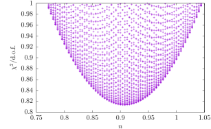
Figure 1: Regions for which $\chi^{2}/d.o.f$ is smaller than 1, for the three statitics used in this letter. The vertical lines indicate the regions allowed in the TOTEM analysis of [2].

All the results shown so far correspond to the usual definition of errors, i.e. the minimum $\chi^{2}$ increases by 1 unit if a parameter is moved by 1 $\sigma$. This definition makes sense for fits with $\chi^{2}$/d.o.f. $\approx 1$. In the present case, the values of $\chi^{2}$ may be too low to use this to determine the parameters. One could for instance allow all the parameter values such that $\chi^{2}$/d.o.f. $\leq 1$. Hence in Fig.˜1, we show the regions with $\chi^{2}/d.o.f$ less than 1 for $\sigma_{tot}$, $\rho$ and $B(0)$ as functions of the normalisation $n$, for the three statistics used in this letter, together with the values of $\chi^{2}/d.o.f.$ of all the points in these regions, this time only for the correlated $\chi^{2}$.

Clearly, the question of the correct value of $n$ is of great impact on the results. We shall proceed with a complementary analysis to settle this question [18].

4 A Bayesian analysis

The data of TOTEM [1] can be translated into two prior probability densities, for $\sigma_{tot}$ and $n$, which we assume gaussian:

$$\mathcal{G}_{1} = {\cal N}_{1}\exp\left(-\frac{(\sigma_{tot}-110.6\ \mathrm{mb})^{2}}{2(3.4\ \mathrm{mb})^{2}}\right)$$ (11)

$$\mathcal{G}_{2} = {\cal N}_{2}\exp\left(-\frac{(n-1.000)^{2}}{2(0.055)^{2}}\right)$$ (12)

with ${\cal N}_{1}$ and ${\cal N}_{2}$ two normalisation so that these probability densities integrate to 1.

We can then define a probability density for the new data

$$\mathcal{L}={\cal N}\exp\left(-\frac{\chi^{2}(x_{k}|d_{i})}{2}\right){\cal G}_{1}{\cal G}_{2}$$ (13)

where $x_{k}$ are our 4 parameters $x_{1}=\sigma_{tot}$, $x_{2}=\rho$, $x_{3}=B$ and $x_{4}=n$, and $\chi^{2}$ is the correlated statistics of Eq. (10), as in ref.˜ [2].

$\cal N$ is defined so that

$$\left[\prod_{k=1,2,3,4}\int dx_{k}\right]{\cal L}=1.$$ (14)

We then consider the probability densities in which we integrate of all parameters but one:

$${d{\cal P}\over dx_{k}}=\left[\prod_{j\neq k}\int dx_{j}\right]{\cal L}.$$ (15)

We then obtain the curves of Fig. 2. We see that the main conclusion of the previous analysis is confirmed: the total cross section is lower than assumed by TOTEM. The other parameters take values similar to those of Table 2 as well, and we give their values in Table 3.

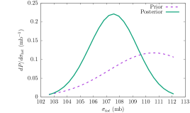
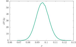
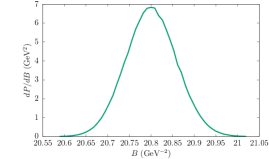
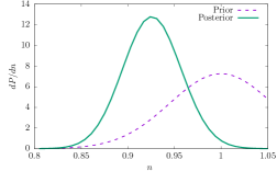
Figure 2: Posterior probabilities of the parameters.

Parameter	Central value	$1\sigma$ error	$2\sigma$ error
$\sigma_{tot}$ (mb)	107.5	$\pm 1.5$	$\pm 2.7$
$\rho$	0.096	$\pm 0.006$	$\begin{subarray}{c}+0.012\\ -0.011\end{subarray}$
$B$ (GeV-2)	20.800	$\pm 0.053$	$\pm 0.097$
$n$	0.924	$\pm 0.028$	$\begin{subarray}{c}+0.041\\ -0.049\end{subarray}$

Table 3: Parameters and errors from the curves of Fig. 2

5 Theoretical error

The total cross section and the $\rho$ parameter are derived quantities obtained via the differential elastic cross section, and as such they depend on the model used to describe elastic scattering [20]. Now the first question is whether the simple form used in Eq. (7 ) provides a good description of the data. One of course has an excellent $\chi^{2}$, but the best way to decide is to consider the residuals, i.e. the difference between the best fit and the data. We show these in Fig. 3.

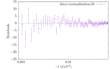
Figure 3: Residuals corresponding to the correlated fit of Table 2.

Clearly, there is no significant departure from an exponential, and the residuals are random. So, in this limited range of $t$, the assumption regarding the form factor matches the data.

However, the form factor enters in a more subtle way, as the phase formula involves integration over the whole $t$ range, and different functional forms lead to different phases. In fact, formula (6) is itself an approximation. We compare its results to the exact form from [17] in Table 3, and also consider the effect of the form factor. The errors are similar to those of Table 2, and the $\chi^{2}$ values are slightly lower, and won’t be quoted here. We see that the form factor has the biggest effect on $\rho$, and that it can increase its value by 0.018.

Form factor	Phase	$\sigma_{tot}$	$\rho$	$n_{i}$
exponential	Eq. (6)	$106.4$	$0.098$	$0.91$
exponential	[17]	$104.1$	$0.106$	$0.87$
dipole	[17]	$106.3$	$0.116$	$0.90$

Table 4: Dependence of the parameters on the formula for the CNI phase, and on the form factor, in the case of a constant $\rho$.

Another assumption in our analysis is that $\rho$ is constant. This is clearly not the case in general [20]. However, one has to realise that only a few points lead to a determination of $\rho$. We show separately in Fig. 4 the contributions to the differential cross section of the hadron amplitude ${\mathcal{A}}_{N}$ and of the Coulomb amplitude ${\mathcal{A}}_{C}$. In the region where the pomeron amplitude dominates, the effect of the real part is small, of order $\rho^{2}\approx 1\%$.

Figure 4: Separate differential cross sections for the hadron contribution, for the Coulomb contribution, and for the total.

There are a few points at the beginning (7 or 8) for which the Coulomb amplitude is not negligible. For those points, at $0.001<|t|<0.003$ GeV², the interference term is present, and it is linear in $\rho$. It is thus this very small interval of momentum that contributes to the determination of $\rho$. Hence assuming a $t$ dependence for $\rho$ does not change the results much. For instance, assuming $\rho=\rho(0)(1+at)$ leads to $\rho(0)=0.099\pm 0.008$ if $a<1$ GeV^-2.

Hence the main source of theoretical error comes from the choice of form factor, and we estimate it at 2 mb on $\sigma_{tot}$ and 0.02 on $\rho$.

6 Conclusion

We have shown that the data of [2] indicate that the measurement of the total cross section of [1] should be lowered by about 1 $\sigma$, and the elastic cross section by about 2 $\sigma$. This has already been pointed out at lower energies, using ATLAS and TOTEM results [17], but as we have shown here, it is true using only TOTEM data.

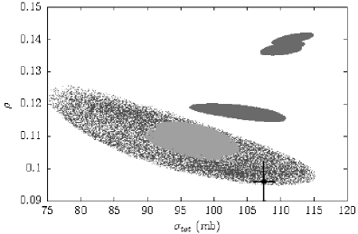
Figure 5: Regions of the ($\sigma_{tot}$, $\rho$) plane allowed at the 1 $\sigma$ level by the COMPETE fits. The upper three regions in dark gray correspond to fits of the form $Z+B\log^{2}(s/s_{0})$, the light gray region to fits of the form $Z+B\log(s/s_{0})$ and the dotted region to fits of the form $A\log^{2}s+B\log s+C$. The experimental point corresponds to the values of the present analysis.

The second point concerns the need for an odderon. We could refit all existing data and check whether this is the case. However, as it turns out, a parametrization published in 2002 [3] agrees with the TOTEM data, without requiring an odderon. From the details of those fits [19], one can reconstruct the 1 $\sigma$ allowed regions in the ($\sigma_{tot}$, $\rho$) plane. We show these regions in Fig. 5. Clearly, some of the parametrisations are ruled out. However, the two parametrisations for which $\sigma_{tot}=A\log^{2}s+B\log s+C$ are allowed and fully compatible with the data. It seems a refit would be a good idea, but the inference that the TOTEM data implies the existence of an odderon seems misguided.

In this letter, we concentrated on the simplest analysis of TOTEM data at 13 TeV. The main drawback is that we totally neglect the analytic properties of the hadronic amplitude, which constrain $\rho$ once the $s$ dependence of the amplitude is known, Such an analysis has however many problems. Even if one concentrates on high-energy data, there is disagreement between TeVatron experiments, and between LHC experiments, making the overall fit necessarily bad. Also, the analysis becomes model-dependent, as one does not know the true high-energy form of the hadronic amplitude. It might be possible to remove some of these problems by considering only TOTEM data, but we leave this to a future work.

References

- [1] G. Antchev et al. [TOTEM Collaboration], CERN-EP-2017-321, CERN-EP-2017-321-V2, arXiv:1712.06153 [hep-ex].
- [2] G. Antchev et al. [TOTEM Collaboration], CERN-EP-2017-335, CERN-EP-2017-335-v3, arXiv:1812.04732 [hep-ex].
- [3] J. R. Cudell et al. [COMPETE Collaboration], Phys. Rev. Lett. 89 (2002) 201801 [hep-ph/0206172].
- [4] L. Lukaszuk and B. Nicolescu, Lett. Nuovo Cim. 8 (1973) 405. K. Kang and B. Nicolescu, Phys. Rev. D 11 (1975) 2461.
- [5] E. Martynov and B. Nicolescu, Phys. Lett. B 778 (2018) 414 [arXiv:1711.03288 [hep-ph]]; E. Martynov and B. Nicolescu, arXiv:1804.10139 [hep-ph].
- [6] http://cerncourier.com/cws/article/cern/71278
- [7] A. Breakstone et al., Phys. Rev. Lett. 54 (1985) 2180.
- [8] S. Gasiorowicz, Elementary particle physics, John Wiley & Soms,Inc, New York - London - Sydney (1967).
- [9] V. Barone and E. Predazzi, High-Energy Particle Diffraction,Springer-Verlag Berlin Heidelberg (2002).
- [10] A.I.Akhiezer and I.Ya.Pomeranchuk, J. Phys. USSR, v.9, p.471 (1945); I.Ya. Pomeranchuk, Sobranie Trudov, v.3, Moscow, Nauka, p.96 (1972) (in Russian).
- [11] H. A. Bethe, Annals Phys. 3 (1958) 190.
- [12] L.D. Soloviev, Zh. Eksp. Teor. Fiz., 49, 292, (1965).
- [13] J. Rix and R. M. Thaler, Phys. Rev. 152 (1966) no.4, 1357. doi:10.1103/PhysRev.152.1357
- [14] M. P. Locher, Nucl. Phys. B 2 (1967) 525.
- [15] G. B. West and D. R. Yennie, Phys. Rev. 172 (1968) 1413.
- [16] V. Kundrat and M. Lokajicek, Phys. Lett. B 611 (2005) 102 doi:10.1016/j.physletb.2005.02.025 [hep-ph/0412081].
- [17] O. V. Selyugin, Phys. Rev. D 91 (2015) no.11, 113003 Erratum: [Phys. Rev. D 92 (2015) no.9, 099901] [arXiv:1505.02426 [hep-ph]]; AIP Conf. Proc. 1819 (2017) no.1, 040017 [arXiv:1611.04313 [hep-ph]].
- [18] R. Andrae, arXiv:1009.2755 [astro-ph.IM]; R. Andrae, T. Schulze-Hartung and P. Melchior, arXiv:1012.3754 [astro-ph.IM].
- [19] The parametrisations used here are (and have been) available at http://nuclth02.phys.ulg.ac.be/compete/publications/benchmarks_details/.
- [20] J.-R. Cudell and O. V. Selyugin, Phys. Rev. Lett. 102 (2009) 032003 [arXiv:0812.1892 [hep-ph]].