Time-optimal purification of a qubit in contact with a structured environment

Abstract

We investigate the time-optimal control of the purification of a qubit interacting with a structured environment, consisting of a strongly coupled two-level defect in interaction with a thermal bath. On the basis of a geometric analysis, we show for weak and strong interaction strengths that the optimal control strategy corresponds to a qubit in resonance with the reservoir mode. We investigate when qubit coherence and correlation between the qubit and the environment speed-up the control process.

I Introduction

Controlling quantum systems with high efficiency in minimum time is of paramount importance for quantum technologies Acín et al. (2018); Brif et al. (2010); Glaser et al. (2015); Altafini and Ticozzi (2012); Dong and Petersen (2010). Since in any realistic process, the system is inevitably subject to an interaction with its environment, it is therefore crucial to understand the fundamental mechanisms allowing to manipulate open quantum systems. A key point is the role that non-Markovianity (NM) Breuer et al. (2016); de Vega and Alonso (2017) can play as resource for control Koch (2016). Several studies have recently pointed out the beneficial role of NM, for instance in the decrease of quantum speed limit or in the protection of entanglement properties Deffner and Lutz (2013); del Campo et al. (2013); Mangaud et al. (2018); Reich et al. (2015); Poggi et al. (2017); Mukherjee et al. (2015).

Quantum optimal control theory (OCT) is nowadays a mature field with applications extending from molecular physics, nuclear magnetic resonance and quantum information processing Brif et al. (2010); Glaser et al. (2015); Altafini and Ticozzi (2012). A variety of numerical optimization algorithms has been developed so far to realize different tasks Werschnik and Gross (2007); Reich et al. (2012); Bryson and Ho (1975); Doria et al. (2011); Kelly et al. (2014); Khaneja et al. (2005); Krotov (1996), but also to account for experimental imperfections and constraints Borneman et al. (2010); Daems et al. (2013); Egger and Wilhelm (2014); Kobzar et al. (2012); Lapert et al. (2009). Originally applied to closed quantum systems, optimal control techniques have become a standard tool for open systems, both in the Markovian and non-Markovian regimes (see Glaser et al. (2015); Koch (2016) and references therein). While OCT is very efficient and generally applicable, it is often not straightforward to deduce the actual control mechanisms. In contrast, geometric and analytic optimal control techniques yield typically more intuitive control solutions for low dimensional systems Agrachev and Sachkov (2004); D’Alessandro (2008); Jurdjevic (1997). Recent studies have shown the potential of such methods both for closed Albertini and D’Alessandro (2015); Assémat et al. (2010); Boscain et al. (2005); Boscain and Mason (2006); D’Alessandro and Dahled (2001); Garon et al. (2013); Khaneja et al. (2001); Sugny and Kontz (2008) and open quantum systems Khaneja et al. (2003b); Bonnard et al. (2009, 2012). In this direction, while the control of a dissipative qubit in the Markovian regime is by now well understood Lapert et al. (2013, 2010); Mukherjee et al. (2013); Tannor and Bartana (1999), very few studies have focused on the case of a structured bath with a possibly non-Markovian dynamics Basilewitsch et al. (2017); Mukherjee et al. (2015). This is due to the inherent complexity of such systems which prevents a geometric analysis.

In order to tackle this control problem, we consider a minimal model of a controlled qubit coupled to a structured environment Basilewitsch et al. (2017). The bath is composed of a well-defined mode, a two-level quantum system (TLS), interacting with a thermal reservoir, that can be described by a Markovian master equation. We assume that the external control field can only modify the effective energy splitting of the qubit. The decisive advantage of this simple control scenario is that a complete geometric and analytical description can be carried out. We generalize Ref. Basilewitsch et al. (2017) where optimal control fields are designed numerically and a geometric description is derived when the interaction between the reservoir mode and the thermal bath is neglected. The generalization allows us to analyze different configurations of the model system geometrically for the whole range of parameters.

As an example control problem, we investigate the maximization of qubit purity in minimum time. Purification is a prerequisite in many applications. Qubit reset has been shown through the coupling with a thermal bath Geerlings et al. (2013); Valenzuela et al. (2006); Reed et al. (2010); Grajcar et al. (2008), but also by other mechanisms Magnard et al. (2018); Jelezko et al. (2004); Johnson et al. (2012); Ristè et al. (2012a, b). A schematic description of the purification process used here is given in Fig. 1. For the model system under study, we analyze the interplay between NM, quantum speed limit and maximum available purity. We show that the time-optimal reset protocol corresponds to a resonant process for any coupling strength between the qubit and the TLS and decay rate of the bath. We also discuss the role of initial coherences and correlations between the qubit and the bath mode and we show that in some specific cases they allow to speed up the control and improve the final purity.

The remainder of this paper is organized as follows. The model system is presented in Sec. II. A specific choice of coordinates allowing to reduce the dimension of the control problem is described. Section III is dedicated to the design of the time-optimal solution for the qubit purification process. The role of initial coherences and correlations is discussed in Sec. IV. We conclude in Sec. V. Some technical formulas and mathematical details are reported in Appendices A and B.

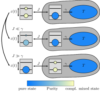
Figure 1: (Color online) Schematic representation of the purification setup: A qubit is coupled to an environmental TLS (with a coupling strength $J$) which decays with the rate $\gamma$ (defined in Eq. (11)) into a heat bath. In the weak coupling limit, which is identified to Markovian dynamics, the state of maximum purity cannot be reached in finite time (middle). If a strong coupling $J$ is considered then the qubit can be directed to the state of maximum purity (bottom).

II Model

We consider a system consisting of a qubit whose effective energy splitting $\omega_{\text{q}}$ can be modified by an external control field $\varepsilon(t)$ Basilewitsch et al. (2017). The corresponding Hamiltonian reads

$$\mathbf{H}_{\text{q}}(t)=-\frac{\omega_{\text{q}}}{2}\bm{\sigma}_{\text{q}}^{z}-\frac{\varepsilon(t)}{2}\bm{\sigma}_{\text{q}}^{z},$$ (1)

where $\bm{\sigma}^{x},\ \bm{\sigma}^{y},\ \bm{\sigma}^{z}$ are the usual Pauli operators. The qubit is possibly strongly coupled to a two-level system (TLS) modelling a representative mode of the environment, giving rise to non-Markovian dynamics. In practice, the model can describe the dynamics of two superconducting qubits in a LC circuit. The dissipation can for example be described by a resistor PhysRevB.94.184503 or by coupling one of superconducting qubits to a lossy cavity PhysRevLett.110.120501. We model the TLS and its interaction with the qubit by the following Hamiltonians,

$$\mathbf{H}_{\text{tls}}=-\frac{\omega_{\text{tls}}}{2}\bm{\sigma}_{\text{tls}}^{z},\qquad\mathbf{H}_{\text{int}}=-J\bm{\sigma}_{\text{q}}^{x}\bm{\sigma}_{\text{tls}}^{x},$$ (2)

where $\omega_{\text{tls}}$ is the frequency of the bath mode and $J$ the coupling strength between the qubit and the TLS. The coupling of the TLS to the rest of the environment is described by a standard Markovian master equation,

$$\textrm{i}\frac{\text{d}}{\text{d}t}\bm{\rho}(t)=\left[\mathbf{H}(t),\bm{\rho}(t)\right]+\bm{\mathcal{L}}_{D}(\bm{\rho}),$$ (3)

$$\bm{\mathcal{L}}_{D}(\bm{\rho})=\textrm{i}\kappa\sum\limits_{k=1,2}\left(\mathbf{L}_{k}\bm{\rho}\mathbf{L}_{k}^{\dagger}-\frac{1}{2}\left\{\mathbf{L}_{k}^{\dagger}\mathbf{L}_{k},\bm{\rho}\right\}\right),$$

where ${\mathbf{H}(t)=\mathbf{H}_{\text{q}}(t)+\mathbf{H}_{\text{tls}}+\mathbf{H}_{\text{int}}}$ is the full Hamiltonian of the qubit and the TLS and $\mathbf{L}_{k}$ the Lindblad operators. In what follows, we will refer to the two parameters $J$ and $\kappa$ as coupling and rate, respectively, to point out their different roles in the purification process, although formally they are of the same nature. We assume the TLS and the bath to be initially in thermal equilibrium characterized by

$$\mathbf{L}_{1}=\sqrt{N+1}\bm{\sigma}_{\text{tls}}^{-},\qquad\mathbf{L}_{2}=\sqrt{N}\bm{\sigma}_{\text{tls}}^{+},$$ (4)

with $N=1/(e^{\beta\omega_{\text{tls}}}-1)$ and $\beta=k_{B}T$, $k_{B}$ and $T$ being, respectively, the Boltzmann constant and the temperature of the bath. $\bm{\sigma}^{-}$ and $\bm{\sigma}^{+}$ are the standard lowering and raising operators for two-level systems. The dynamics of the qubit alone can be extracted as a partial trace over the TLS,

$$\bm{\rho}_{\text{q}}=\text{Tr}_{\text{tls}}(\bm{\rho}).$$ (5)

The density matrix of the joint system, i.e., qubit and TLS, is a $4\times 4$ Hermitian matrix which can be parameterized as

$$\bm{\rho}=\begin{pmatrix}x_{1}&x_{5}+\textrm{i}x_{6}&x_{7}+\textrm{i}x_{8}&x_{9}+\textrm{i}x_{10}\\ x_{5}-\textrm{i}x_{6}&x_{2}&x_{11}+\textrm{i}x_{12}&x_{13}+\textrm{i}x_{14}\\ x_{7}-\textrm{i}x_{8}&x_{11}-\textrm{i}x_{12}&x_{3}&x_{15}+\textrm{i}x_{16}\\ x_{9}-\textrm{i}x_{10}&x_{13}-\textrm{i}x_{14}&x_{15}-\textrm{i}x_{16}&x_{4}\end{pmatrix},$$ (6)

where the $x_{i}$ are real coefficients and $\sum_{i=1}^{4}x_{i}=1$. The dynamical space of the system therefore has 15 dimensions. After applying the rotating wave approximation (RWA), see Appendix A, the dynamics can be separated into four uncoupled subspaces. Only two of these contribute to the qubit purity in which we are interested in, the other two are therefore neglected. Technical details about the structure of the dynamical space are given in Appendix B. The definition of the subspaces is clarified by introducing a new set of parameters:

$$\begin{aligned} z_{1}&=x_{1}+x_{2}-1/2,&z_{5}&=x_{7}+x_{13},\\ z_{2}&=x_{12},&z_{6}&=x_{6}-x_{16},\\ z_{3}&=x_{11},&z_{7}&=x_{8}+x_{14},\\ z_{4}&=-2x_{1}-x_{2}-x_{3},&z_{8}&=x_{5}-x_{15},\end{aligned}$$ (7)

in which the qubit purity reads

$$P_{\text{q}}=\frac{1}{2}+2\left(z_{1}^{2}+z_{5}^{2}+z_{7}^{2}\right).$$ (8)

We denote the subspaces associated with the coordinates $(z_{1},z_{2},z_{3},z_{4})$ and $(z_{5},z_{6},z_{7},z_{8})$ by $S_{1}$ and $S_{2}$ . $S_{1}$ describes the population of the qubit and its correlation with the TLS, while $S_{2}$ contains information about the coherences of the qubit and the TLS. The equations of motion on $S_{1}$ and $S_{2}$ are given by

$$\begin{pmatrix}\dot{z}_{1}\\ \dot{z}_{2}\\ \dot{z}_{3}\\ \dot{z}_{4}\end{pmatrix} =2J_{1}\begin{pmatrix}z_{2}\\ -z_{1}-\frac{z_{4}+1}{2}\\ 0\\ 0\end{pmatrix}+2J_{2}\begin{pmatrix}z_{3}\\ 0\\ -z_{1}-\frac{z_{4}+1}{2}\\ 0\end{pmatrix}$$

$$\quad+2\alpha\begin{pmatrix}0\\ -z_{3}\\ z_{2}\\ 0\end{pmatrix}-\gamma\begin{pmatrix}0\\ \frac{z_{2}}{2}\\ \frac{z_{3}}{2}\\ \frac{\gamma_{1}}{\gamma}+z_{1}+z_{4}+\frac{1}{2}\end{pmatrix},$$ (9)

and

$$\begin{pmatrix}\dot{z}_{5}\\ \dot{z}_{6}\\ \dot{z}_{7}\\ \dot{z}_{8}\end{pmatrix} =J_{1}\begin{pmatrix}z_{6}\\ -z_{5}\\ -z_{8}\\ z_{7}\end{pmatrix}+J_{2}\begin{pmatrix}-z_{8}\\ z_{7}\\ -z_{6}\\ z_{5}\end{pmatrix}$$

$$\quad+2\alpha\begin{pmatrix}z_{7}\\ 0\\ -z_{5}\\ 0\end{pmatrix}-\frac{\gamma}{2}\begin{pmatrix}0\\ z_{6}\\ 0\\ z_{8}\end{pmatrix},$$ (10)

where we have introduced

$$\begin{gathered}\begin{aligned} \delta(t)&=\omega_{\text{q}}+\varepsilon(t)-\omega_{\text{tls}},\quad&\alpha(t)&=\frac{t}{2}\frac{\text{d}\delta}{\text{d}t},\\ J_{1}&=J\cos\left({\delta t}\right),&J_{2}&=J\sin\left({\delta t}\right),\\ \gamma_{1}&=\kappa(N+1),&\gamma_{2}&=\kappa N,\\ \end{aligned}\ \\ \text{with }\gamma=\gamma_{1}+\gamma_{2}.\end{gathered}$$ (11)

From a geometric point of view, $S_{1}$ is a 2-dimensional sphere in the space $(z_{1},z_{2},z_{3})$ defined by

$$(z_{1}-c)^{2}+z_{2}^{2}+z_{3}^{2}=r(\gamma)$$ (12)

with its center $c=-(z_{4}+1)/2$ moving along the $z_{1}$-axis and radius $r$ decreasing with rate $\gamma$. $S_{2}$ describes a 3-dimensional sphere in the space $(z_{5},z_{6},z_{7},z_{8})$ given by

$$z_{5}^{2}+z_{6}^{2}+z_{7}^{2}+z_{8}^{2}=r^{\prime}(\gamma)$$ (13)

with a fixed center at the origin and decreasing radius $r^{\prime}$.

The initial state is constructed from the tensor product of the two separate density matrices Basilewitsch et al. (2017)

$$\begin{aligned} \bm{\rho}=&\bm{\rho}_{\text{q}}\otimes\bm{\rho}_{\text{tls}}+\bm{\rho}_{\text{corr}}\\ =&\begin{pmatrix}a_{\text{q}}&\mu_{\text{q}}+\textrm{i}\nu_{\text{q}}\\ \mu_{\text{q}}-\textrm{i}\nu_{\text{q}}&b_{\text{q}}\end{pmatrix}\otimes\begin{pmatrix}a_{\text{tls}}&0\\ 0&b_{\text{tls}},\end{pmatrix}\\ &+\begin{pmatrix}0&0&0&0\\ 0&0&\textrm{i}\xi&0\\ 0&-\textrm{i}\xi^{*}&0&0\\ 0&0&0&0\end{pmatrix},\end{aligned}$$ (14)

where $a_{k}$ and $b_{k}$ are the ground- and exited state populations of qubit and TLS in thermal equilibrium, which are defined by their respective energy level splittings $\omega_{k}$ and the temperature. They can be expressed explicitly as ${a_{k}=\frac{e^{\beta\omega_{k}/2}}{2\ \cosh\left(\beta\omega_{k}/2\right)}}$ and $b_{k}=1-a_{k}$. The parameters $\mu_{\text{q}}$ and $\nu_{\text{q}}$ are the coherences in the reduced state of the qubit. We neglect coherences of the TLS assuming that it is initially in a thermal state. Our analysis could also be carried out for a non-thermal initial qubit population. Furthermore, we artificially add coherences between the qubit and the TLS with the extra term $\bm{\rho}_{\text{corr}}$. Since coherences $\xi$ give rise to correlations between the qubit and the TLS, we refer to these coherences as correlations throughout the paper.

If not stated otherwise, the parameters are set to ${\omega_{\text{q}}=1,\ \omega_{\text{tls}}=3,\ \beta=1,\ J=0.1}$ throughout as in Ref. Basilewitsch et al. (2017), allowing for a qualitative comparison of the results, but in principle the parameters can be chosen arbitrarily. The only constraint on the frequencies is $\omega_{\text{q}}<\omega_{\text{tls}}$ in order for the qubit purity to be initially lower than the TLS purity. The coupling strength $J$ obeys $J\ll\omega_{\text{q}}$ in order to satisfy the different approximations made to establish the model system Basilewitsch et al. (2017).

III Purification of a qubit in a thermal state

In this section, we focus on the purification of a qubit in a thermal state. This means, in particular, that the qubit has no initial coherence (${\mu_{\text{q}}=\nu_{\text{q}}=0}$) and all variables $z_{5},\dots,z_{8}$ and their time derivatives vanish, see Eqs. (7), (II) and (14). Therefore, we need to only consider the dynamics in $S_{1}$, governed by Eq. (II), and neglect contributions from $S_{2}$ for now. As a consequence, maximizing the purity $P_{\text{q}}$, see Eq. (8), simplifies to maximizing $z_{1}$. In this case, using the spherical symmetry, the dynamics can be further simplified by introducing spherical coordinates,

$$\begin{gathered}c=-\frac{z_{4}+1}{2},\\ r\sin\left({\theta}\right)=z_{1}-c,\\ r\cos\left({\theta}\right)\sin\left({\varphi}\right)=z_{2},\\ r\cos\left({\theta}\right)\cos\left({\varphi}\right)=z_{3}.\end{gathered}$$ (15)

Note that $r$ is identical with the one in Eq. (12). The full dynamics of the qubit in these coordinates are then described by

$$\dot{r} =-\frac{\gamma}{2}\left(r+(\eta-c)\sin\left({\theta}\right)\right),$$ (16a)

$$\dot{c} =\frac{\gamma}{2}\left(r\sin\left({\theta}\right)+(\eta-c)\right),$$ (16b)

$$\dot{\theta} =-\frac{\gamma}{2}\frac{\eta-c}{r}\cos\left({\theta}\right)+2J\cos\left({\delta t-\varphi}\right),$$ (16c)

$$\dot{\varphi} =2\alpha-J\tan\left({\theta}\right)\sin\left({\delta t-\varphi}\right),\vphantom{\frac{\gamma}{2}}$$ (16d)

where $\eta=\gamma_{1}/\gamma-1/2$ and the control field $\varepsilon(t)$ (see Eq. (1)) is present in the quantities $\delta(t)$ and $\alpha(t)$.

Since we do not assume any initial coherence of the qubit, the qubit’s purity $P_{\text{q}}$ is completely determined by the dynamics on $S_{1}$. Using the spherical coordinates of Eq. (15), it can be expressed as

$$P_{\text{q}}=\frac{1}{2}+2(r\sin\left({\theta}\right)+c)^{2}.$$ (17)

Because $\varphi$ does not enter into the purity, we can define a new control,

$$u(t)=\delta t-\varphi.$$ (18)

Using Eq. (16d), we arrive at

$$\delta=\dot{u}-J\tan\left({\theta}\right)\sin\left({u}\right).$$ (19)

This way we can first determine the optimal control strategy for $u(t)$ and afterwards calculate the physical controls $\delta(t)$, respectively $\varepsilon(t)$.

The North Pole of the $S_{1}$ sphere defined by $\theta=\pi/2$ is the state of maximum purity, and we will denote its position on the $z_{1}$-axis by $Z=r+c$. In principle, the maximum accessible purity can change over time since the radius $r$ and the center $c$ of the sphere change. The time evolution of $Z$ is governed by

$$\dot{Z} =\dot{r}+\dot{c}=-\frac{\gamma}{2}(Z-\eta)\underbrace{(1-\sin\left({\theta}\right))}_{\geq 0}.$$ (20)

Using Eqs. (11) and (14), it is straightforward to show that ${\eta=a_{\text{tls}}-\frac{1}{2}}$. This quantity can be connected to the initial TLS purity as $P_{\text{tls}}(0)=\frac{1}{2}+2\eta^{2}$. The behavior of $Z$ is different depending on whether qubit and TLS are initially correlated or not. Hence, we examine both cases separately in the following.

III.1 Time-optimal control in the correlation-free case

If there is no initial correlation between qubit and TLS ($\xi=0$), we find the relation ${Z=a_{\text{tls}}-\frac{1}{2}=\eta}$ by evaluating the initial state given by Eq. (14) in terms of the coordinates of Eqs. (7) and (15). We therefore deduce from Eq. (20) that $Z$, the North Pole of $S_{1}$, is a constant of motion for correlation-free initial states. Moreover, this constant can be used to simplify the differential system (16) even further by replacing ${c=Z-r=\eta-r}$. Effectively, the dynamics can then be described by only two equations

$$\dot{r} =-\frac{\gamma}{2}r\left(1+\sin\left({\theta}\right)\right),$$ (21a)

$$\dot{\theta} =-\frac{\gamma}{2}\cos\left({\theta}\right)+2J\cos\left({u}\right).$$ (21b)

Without correlation ($\xi=0$, implying $z_{2}=z_{3}=0$), the initial state of the system is the South Pole ($\theta=-\pi/2$) of $S_{1}$ as it can be verified with Eq. (15). Since $Z$ is a constant of motion, the control strategy consists in performing a rotation to reach the North Pole ($\theta=\pi/2$) of the sphere as fast as possible. In the dissipation-free case ($\gamma=0$), the radius becomes constant and $\theta$ is rotating with velocity $\dot{\theta}=2J\cos u$ (see Eq. (21b)). The maximum speed for the rotation is reached with $u(t)=0$ which corresponds to the resonant case $\delta(t)=0$ (see Eq. (19)). This control strategy does not change if the dissipation is taken into account. However, the dissipative term slows down the rotation, which can be seen by the relative opposite signs of the two terms in Eq. (21b). Two scenarios can be encountered according to the relative weights of the two terms, one in which the dissipation dominates and a second where it can be viewed as a perturbation of the unitary dynamics.

In general, we observe that the radius decreases exponentially while the position $c$ of the center approaches asymptotically the value $\eta$. These trajectories define the purity which can be reached by setting the position of the north pole. On the other hand, the angular differential equation (16c) gives us information about the minimum time needed to reach the state of maximum purity. For correlation-free initial states, the angular equation (see Eq. (21b)) can be integrated analytically leading to the minimum time $T_{\textrm{min}}$, which is needed to reach maximum purity on $S_{1}$,

$$T_{\textrm{min}} =\int\limits_{-\pi/2}^{\pi/2}\frac{\text{d}\theta}{\dot{\theta}}=\frac{8\arctan\left({\sqrt{\frac{4J+\gamma}{4J-\gamma}}}\right)}{\sqrt{(4J+\gamma)(4J-\gamma)}}.$$ (22)

In the zero dissipation limit $\gamma\rightarrow 0$, we recover the result established in Ref. Basilewitsch et al. (2017) of ${T_{\textrm{min}}(\gamma=0)=T_{0}=\frac{\pi}{2J}}$. From Eq. (22) it can be seen that the case $J\leq J_{\text{min}}$, with

$$J_{\text{min}}=\gamma/4,$$ (23)

is not well defined. This scenario corresponds to the already mentioned case in which the dissipation dominates, which can be attributed to the change from non-Markovian to Markovian qubit dynamics. In the latter case, the dissipative term becomes too large and a fixed point in $\theta$, i.e., $\dot{\theta}=0$, given by $\theta_{\text{f}}=\arccos\left({4J/\gamma}\right)$ arises. At the fixed point, correlations between the qubit and TLS, which are build up during the process, cannot be transformed into population anymore and therefore do not further contribute to the purification. The North Pole is thus not accessible and any gain in purification comes only from the exponential decrease in $r$ caused by the dissipation into the heat bath, see Fig. 2(c). This is a remarkable feature, because naively the decrease of $r$ due to dissipation would be connected to a loss of purity. Since the decrease in $r$ is maximized, in this case, for $\theta=\theta_{\text{f}}$, the optimal strategy consists here again in applying a zero control field $u(t)=0$. However, the final state cannot be reached in finite time. Using a standard measure of non-Markovianity Lorenzo et al. (2013), we have also verified that the different parameter regions can indeed be identified with the Markovian ($\gamma>4J$) and non-Markovian regimes ($\gamma<4J$).

The trajectories for the non-Markovian and Markovian cases are plotted in Fig. 2(a) and (c). Figure 3 displays the dependence of the minimum time on the ratio $\gamma/J$ for correlated and uncorrelated initial states. The sharp transition to the Markovian regime can be observed at $\gamma=4J$, indicated by the divergence of the purification time. Figure 3 shows that the purification time for correlated initial states is lower than for uncorrelated ones. As can be seen in Fig. 2(b), this is a consequence of the position of the initial state which is closer to the equator of $S_{1}$.

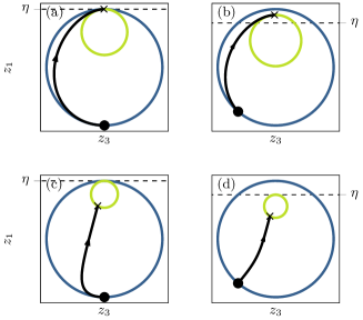
Figure 2: (Color online) Optimal trajectories (in black) of the qubit in the $(z_{1},z_{3})$ - plane without(a) and with correlations (b) for non-Markovian dynamics. The initial and final states are represented, respectively, by a dot and a cross. In panels (c) and (d), the asymptotic steady states are indicated by circles. The blue (dark gray) and green (light gray) circles are the projections onto $(z_{1},z_{3})$ - plane of $S_{1}$ at the initial and final times. The amount of correlations added is equal to the maximum possible value $\xi=\xi_{\text{max}}$ (see Eq. (24)) and $J=4\,J_{\text{min}}$. Panel (c) shows the trajectory for the correlation-free Markovian case ($J=J_{\text{min}}/2$), while the correlated case is displayed in panel (d).

III.2 Time-optimal control with correlated states

Adding $\xi$ - correlations between qubit and TLS to the initial state (14) changes the dynamics because $Z(0)\neq\eta$ and therefore $Z$ is not constant anymore, as shown in Eq. (20). Although it makes a difference whether $\xi$ is real or imaginary, we will only consider real $\xi$ in what follows. This is because a purely imaginary $\xi$ only modifies the initial value of $\varphi$. The control field can always be chosen so that it produces a short and strong $\alpha$-pulse in order to rotate $\varphi$ to $0$, see Eq. (16d) and Ref. Basilewitsch et al. (2017). Since this rotation can be made arbitrarily fast (at least theoretically), we focus on the time-optimal solution for the remaining control problem which coincides with the case of initially real $\xi$.

Arbitrarily large correlations cannot be introduced due to the physical constraint of the density matrix being positive semi-definite. An eigenvalue analysis reveals that the maximum amount of correlation is

$$\xi_{\text{max}}=\sqrt{a_{\text{q}}a_{\text{tls}}b_{\text{q}}b_{\text{tls}}}.$$ (24)

The dynamics of the maximal reachable purity depends on the initial value of $Z-\eta$. Using the definition of the initial state (14), we find

$$Z(0)-\eta=\sqrt{\left(\frac{a_{\text{tls}}-a_{\text{q}}}{2}\right)^{2}+\xi^{2}}-\frac{a_{\text{tls}}-a_{\text{q}}}{2}\geq 0,$$ (25)

from which together with Eq. (20), we can conclude that ${\dot{Z}\leq 0}$ and

$$Z(t)-\eta=(Z(0)-\eta)\exp\left[-\frac{\gamma}{2}\int_{0}^{t}(1-\sin\left({\theta}\right))\text{d}t^{\prime}\right].$$ (26)

Correlations therefore increase the initially accessible purity which then decays asymptotically to $\eta$, the same value as in the uncorrelated case. This decay is caused by the decrease of the radius $r$, which can be written as

$$\dot{r}=-\frac{\gamma}{2}[\underbrace{Z-c}_{=r}+(\eta-c)\sin\left({\theta}\right)].$$ (27)

To prove that $r$ is monotonically decreasing, we distinguish two cases.

• $\eta-c\geq 0$:
  In this situation, together with Eq. (26), we can estimate

  $$\dot{r}\leq-\frac{\gamma}{2}\left(\eta-c\right)\left(1+\sin\left({\theta}\right)\right)\leq 0.$$ (28)

• $\eta-c\leq 0$:
  From Eq. (16b), we can deduce the maximum of $c$ during the process as

  $$c_{\text{max}}=r\sin\left({\theta}\right)+\eta\leq r+\eta.$$ (29)

  Using this relation, an upper limit for $\dot{r}$ is given by:

  $$\dot{r}=-\frac{\gamma}{2}\left(r+\underbrace{\left(\eta-c\right)\sin\left({\theta}\right)}_{\geq-r}\right)\leq 0.$$ (30)

As before, we study the time needed to reach the state of maximum purity by examining the angular dynamics which are governed by (see Eq. (16c))

$$\dot{\theta}=\frac{\gamma}{2}\frac{Z-\eta}{r}\cos\left({\theta}\right)-\frac{\gamma}{2}\cos\left({\theta}\right)+2J\cos\left({u}\right).$$ (31)

Equation (31) is similar to the correlation-free version (21b) but added by a new term, which is always positive in the region of interest $\theta\in[-\pi/2,\pi/2]$. As before, the latter driving term is strongest for $u(t)=0$. The purification time is lower than in the uncorrelated case due to the additional first positive term, which increases the effective driving speed. In addition, correlations change the initial state for $\theta$ given by $\theta(0)=\arccos\left(\xi/r(0)\right)$, which leads to a shorter distance towards the $S_{1}$ north pole to be covered. In particular, the minimum time for $\gamma=0$ is $T_{0}=\frac{\pi/2-\theta(0)}{2J}$. The angular dynamics (31) cannot be integrated analytically anymore, but Fig. 3 shows the numerically calculated times in comparison to the analytical results in the correlation-free case. Interestingly the same divergence for $\gamma>4J$, which corresponds to the transition between Markovian and non-Markovian behavior, can be observed. Physically, this means that if the dissipation becomes too large in comparison with the coupling $J$, the dynamics become Markovian and purification takes an infinite amount of time. The optimal trajectory for the Markovian case is plotted in Fig. 2(d). Nevertheless, we observe that the final state has a lower purity than the initial North Pole even in the case of non-Markovian dynamics. This is due to the decrease of $Z$ over time. However, the final purity is still higher than in the correlation-free case, i.e., with $\xi=0$. The optimal trajectory for this situation is shown in Fig. 2(b).

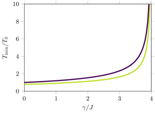
Figure 3: (Color online) Normalized minimum time $T_{\textrm{min}}/T_{0}$ to reach the north pole of $S_{1}$ as a function of $\gamma/J$ for the correlated (green or light gray) and uncorrelated (purple or dark gray) initial states. $T_{0}$ is the purification time for $\gamma=0$ and the parameter $\xi$ is set to $\xi_{\text{max}}$ in the correlated case.

III.3 Role of initial correlations for the existence of a fixed point

Despite being able to reach higher purity in a shorter time, the non-Markovian regime has the drawback the state of maximal purity not being stable. Therefore, after reaching the target state, qubit and TLS have to be decoupled or the purity of the qubit will decrease. This is not the case for Markovian dynamics as shown in Fig. 2(c). The angular fixed point is reached and the system tends continuously to the state of maximum purity, which is in return never reached exactly in finite time.

Figure 4: (Color online) Purification time as a function of the temperature. Panel (a) represents the correlation-free initial state in which we observe the same behavior as in Fig. 3. For a specific threshold, the purification time diverges. If correlations are added (panel (b)) then the angular fixed point is resolved and the target state can be reached in finite time. $\xi=\xi_{\text{max}}$ fixed, but its value depends on $\beta$. The parameter $T_{0}$ was chosen as $T_{0}(\xi=0)$ in panel (b) for the sake of comparison with panel (a).

Figure 4 displays the dependence of the purification on the inverse temperature for uncorrelated and correlated initial states. For large $\beta$, we approach the same purification time in the two situations because the amount of allowed correlations goes to zero in this limit (see Eq. (24)). The minimum time $T_{\textrm{min}}$ is slightly larger than $T_{0}$ due the dissipation terms which are different from zero even at low temperature (see Eq. (11)),

$$\lim\limits_{\beta\rightarrow\infty}{\gamma}=\kappa\neq 0.$$ (32)

Surprisingly, the dynamics have a different behavior for small $\beta$. In Fig. 4(a), the transition to the Markovian regime is similar to the one of Fig. 3 with a divergence of the purification time. For correlated initial states (Fig. 4(b)), we observe that for low temperatures, i.e. large $\beta$, the purification time decreases and approaches zero. This suggests that the angular fixed point can be resolved by adding correlations, as described below.

The following discussion describes the behaviour of ${\dot{\theta}=0}$. We will refer to the value of $\theta$ at which its derivative vanishes as angular fixed point $\theta_{\text{f}}$, although it is not a fixed point of the full dynamics i.e. a steady state.

For correlated initial states, the fixed point equation reads

$$\theta_{\text{f}}=\arccos\left({\frac{4J}{\gamma}\frac{r}{\eta-c}}\right)=\arccos\left({\frac{4J}{\gamma}\frac{Z-c}{\eta-c}}\right).$$ (33)

Note that the value of $\theta_{\text{f}}$ depends on $r$ and $c$ and therefore can change over time. It is only a fixed point in the sense that if ${\theta=\theta_{\text{f}}}$ is reached, it will not change its value anymore, even though $r$ and $c$ will still continue to vary.

This fixed point is only defined if $\frac{4J}{\gamma}\frac{r}{\eta-c}>1$, otherwise there is no solution to Eq. (33) and no fixed point occurs. Recall that, for uncorrelated initial states, we found ${Z=\eta}$ and therefore we recover $J\leq\frac{\gamma}{4}$ as the condition for the existence of the fixed point. In general, as can be seen from Eq. (25), the second term is always larger or equal to one and $J>\frac{\gamma}{4}$ leads to fixed point-free dynamics. However, if initial correlations between qubit and TLS are introduced, the fixed point can be resolved for $J<\frac{\gamma}{4}$. From Eq. (33), we can calculate the maximum amount of correlations for which the fixed point is still defined,

$$\xi_{\text{fixed}}=\pm\frac{a_{\text{tls}}-a_{\text{q}}}{2}\sqrt{1-\left(\frac{\gamma}{4J}\right)^{2}}.$$ (34)

If more correlations are included, there is no fixed point present initially. Nevertheless, a fixed point, into which the dynamics may eventually run, can still occur during the time evolution itself.

Figure 5 displays the dynamics of $\theta$ and the time evolution of the value of $\theta_{\text{f}}$. It can be seen that exceeding the preceding bound (34) even further (i.e. comparing Fig. 5(a) and (b)) prevents the fixed point from arising also during the time evolution. The system can reach the angle $\theta=\pi/2$ and therefore the state of maximum purity in finite time. In contrast to correlation-free initial states, this conclusion is true for any temperature with sufficient initial correlations. Note that the limiting boundary for a valid density matrix has to be satisfied.

In general, the dynamics of the system can be split into different regimes, depending on the correlations, which are shown in Fig. 6. The different zones describe the regime in which no fixed point is present initially, the case where the fixed point arises during the evolution and the region in which no fixed point occurs during the whole purification process. Interestingly, we can go from one regime to the other by controlling the amount of correlations between the qubit and the TLS. Although it is possible to purify the system in region C in finite time, as it is in the non-Markovian regime, it is important to point out that non-Markovianity is a feature of the dynamical map, which does not depend on the initial state Dajka et al. (2011); Smirne et al. (2010); Wißmann et al. (2013).

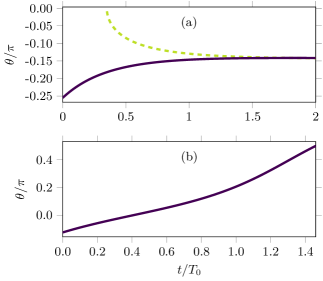
Figure 5: (Color online) Time evolution (solid line) of the angle $\theta$ in the Markovian regime $J=0.9\,J_{\text{min}}$ (cf. Eq. (23)). The correlations are set to $\xi=2\,\xi_{\text{fixed}}$ and $\xi=5\,\xi_{\text{fixed}}$ in panels (a) and (b), respectively. The dashed green line in panel (a) depicts the position of the fixed point $\theta_{\text{f}}$.

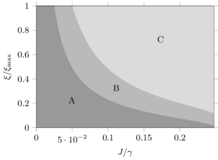
Figure 6: Existence of an angular fixed point in $\theta$ as a function of correlation and coupling strength ($\beta=0.1$). In region A, a fixed point is initially defined, while in region B there no fixed point accessible initially, but during the time evolution of the system. Area C corresponds to the parameter space in which no fixed point occurs in the time in which the final state is reached.

IV Role of initial coherences and correlations for the control strategy

We investigate in this section the joint influence of correlations in the presence of initial qubit coherences, i.e., $\mu_{\text{q}},\nu_{\text{q}}\neq 0$, on the optimal strategy designed in Sec. III. In particular, qubit coherences lead to a dynamics on $S_{2}$ since $z_{5}$ or $z_{7}$ are not vanishing anymore, see Eq. (7) and (II). Hence, the qubit purity $P_{\text{q}}$ gets now simultaneous contributions from both spheres. Using Eq. (8), the purity can be split into two different contributions. The terms proportional to $z_{1}^{2}$ will be called contribution from $S_{1}$ and the other terms will be assigned to $S_{2}$.

Therefore, it is interesting to study whether the dynamics on $S_{2}$ change the procedure to get the highest overall purity $P_{\text{q}}$. For the resonant case, $\delta=\alpha=0$, the equations on $S_{2}$ are

$$\dot{z}_{5} =Jz_{6},$$ (35a)

$$\dot{z}_{6} =-Jz_{5}-\frac{\gamma}{2}z_{6},$$ (35b)

$$\dot{z}_{7} =-Jz_{8},$$ (35c)

$$\dot{z}_{8} =Jz_{7}-\frac{\gamma}{2}z_{8},$$ (35d)

with the initial conditions

$$z_{5}(0) =\mu_{\text{q}}, z_{7}(0) =\nu_{\text{q}},$$

$$z_{6}(0) =0, z_{8}(0) =0.$$ (36)

Because the equations for $z_{5}$ and $z_{7}$ are decoupled and only their squared sum enters into the purity, it is sufficient to consider $z_{7}=0$ or equivalently only real coherences. The equations of motion are identical to the ones of a damped harmonic oscillator. The solution reads

$$z_{5}(t)=\mu_{\text{q}}\sqrt{1+\left(\frac{\gamma}{4\omega}\right)^{2}}\cos\left({\omega t-\arctan\left({\frac{\gamma}{4\omega}}\right)}\right){\rm e}^{-\frac{\gamma}{4}t},$$ (37)

with $\omega=\sqrt{J^{2}-\gamma^{2}/16}$. This describes an oscillating behavior damped by an exponential decay having its maximum at $t=0$. The purity contribution from $S_{2}$ is therefore maximal in the initial state. As in Sec. III, we can identify the Markovian limit $\gamma\geq 4J$ in which the cosine function turns into a hyperbolic cosine and $z_{5}$ is monotonically decreasing. We focus below only on the non-Markovian case. Caution has to be made on the allowed range of parameters $\mu_{\text{q}}$ and $\xi$. For vanishing coherences, the maximum value of $\xi$ has already been calculated in Eq. (24) and this computation can be done for $\mu_{\text{q}}$ in a similar way. If both coherences and correlations are present then the limits are determined numerically. We compute the maximum value of $\mu_{\text{q}}$ for which the density matrix for a given $\xi$ has non-negative eigenvalues. The allowed parameter region is plotted in Fig. 7.

At this point, we already know how to maximise the purity contributions from $S_{1}$ and $S_{2}$ separately. It is however not clear how the overall purity behaves. We again consider the cases of correlated and uncorrelated initial states separately.

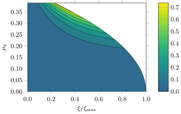
Figure 7: (Color online) Parameter space of the correlations $\xi$ and coherences $\mu_{\text{q}}$ for which the density matrix is defined. The color code indicates the relative difference (Eq. (38)) between the maximum purity reached during the evolution and the purity at ${\theta=\pi/2}$ in per cent.

In the uncorrelated situation, we combine Eqs. (22) and (37) to observe that, at time $T_{\textrm{min}}$, where the purity is maximum on $S_{1}$, the contribution of $S_{2}$ vanishes i.e. $z_{5}(T_{\textrm{min}})=0$. The corresponding trajectory is plotted in Fig. 8(a). As shown in Fig. 9(a), numerical simulations reveal that the dynamics on $S_{2}$ are not relevant at all since the maximum purity and the time to reach it are the same as the ones on $S_{1}$ for any value of $\mu_{\text{q}}$. In particular, the best final purity is limited by the initial purity of the TLS.

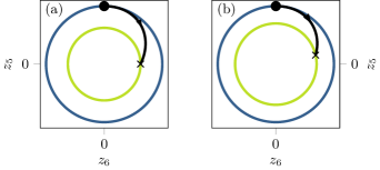
Figure 8: (Color online) Optimal trajectories on $S_{2}$ in the $(z_{5},z_{6})$- plane without (a) and with (b) initial correlations. The initial and final points are represented, respectively, by a dot and a cross. The control time is set to $T_{\text{min}}$, see Eq. (22). Parameters are set to $\xi=\xi_{\text{max}}/2$ and $\mu_{\text{q}}=\mu_{\text{q, max}}$. Note that $\mu_{\text{q, max}}$ depends on $\xi$. The blue (dark gray) and green (light gray) circles are the projections of $S_{2}$ onto the $(z_{5},z_{6})$- plane at initial and final times.

However, this behavior changes if correlations are considered. As can be seen in Eq. (35), they do not affect the dynamics on $S_{2}$ but they reduce the time needed to reach the north pole on $S_{1}$ and therefore introduce a phase shift between $S_{1}$ and $S_{2}$. Due to this shorter time, the contribution from $S_{2}$ has not completely vanished yet and the overall purity can increase, see Fig. 8(b). This maximum amount of purity, which is reached during the purification process, is called $P_{\text{max}}$. The color code in Fig. 7 indicates

$$\Delta P=\frac{P_{\text{max}}}{P(T_{\text{min}})}-1.$$ (38)

This corresponds to the relative purity which is gained by taking into account the combined dynamics of $S_{1}$ and $S_{2}$. The numerical results of Fig. 9(b) demonstrate that, in case of initial correlations, qubit coherences can be transformed into an additional gain of population and therefore break the limit of the TLS purity. Note that this is not possible with correlation-free initial states as shown in Fig. 8(a) and 9(a). Moreover, it can be seen in Fig. 9(b) that, while the maximally accessible purity increases, the minimum time needed to reach it decreases as coherences increase. In other words, qubit coherences improve both total time and final purity of the control scheme, but require qubit and TLS to be initially correlated.

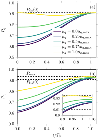
Figure 9: (Color online) Time evolution of the qubit purity $P_{\text{q}}$ of the qubit for uncorrelated (a) and correlated (b) initial states with different coherences $\mu_{\text{q}}\in[0,\mu_{\text{q,max}}]$, where $\mu_{\text{q,max}}$ is the maximum allowed value of the coherence. The parameter $\xi$ is set to $0$ and $\xi_{\text{max}}/2$ in (a) and (b) respectively. The horizontal dashed lines depict the initial purity of the TLS, $P_{\text{tls}}(0)$ and the maximum value $P_{\textrm{max}}$ of $P_{\text{q}}$.

V Conclusions

We have investigated control of a qubit coupled to a structured reservoir, which is composed of a well-defined and strongly coupled mode and a thermal bath. This model can be realized experimentally with superconducting qubits. We assume that only the energy splitting of the qubit can be changed by the external control field. Using a geometric description of the control problem, we show that the time-optimal protocol to purify the qubit is based on fulfilling a resonance condition between the qubit and the reservoir mode. This result is valid for any coupling strength between the qubit and the environment and for any decay rate of the thermal bath. Non-Markovianity of the qubit dynamics does not modify the control strategy, but reduces the time to reach the state of maximum purity. Introducing strong correlations between qubit and TLS accelerates the process even further. The role of initial qubit coherences has been investigated as well: Combined correlations and qubit coherences speed up the control process and improve the final purity of the qubit even more.

Our study and the possibility to describe geometrically purification of a qubit in contact with a structured reservoir pave the way to future investigations. In particular, it would be interesting to generalize this model to more complex control scenarios in which the external field can be applied also in other directions. For instance, the qubit coherence can be modified by a $\sigma_{x}$- control, which could be combined with the $\sigma_{z}$- control used here to enhance or speed up the purification process. Another intriguing avenue is the application of this approach to algorithmic cooling (AC) in which similar model systems are considered Raeisi and Mosca (2015); Rodríguez-Briones and Laflamme (2016); Rodríguez-Briones et al. (2017). To the best of our knowledge, AC methods neglect the interaction between the bath and the qubits during the first step of the cooling, i.e. the entropy exchange. This approximation could be avoided by generalizing the results of this work to the case of $n$ qubits ($n>1$) and $m$ reset qubits or modes ($m\geq 1$).

Appendix A Rotating wave approximation

Starting from the Hamiltonian governing the dynamics of the model system,

$$\mathbf{H}(t)=\underbrace{-\frac{\omega_{\text{q}}+\varepsilon(t)}{2}\ \bm{\sigma}_{\text{q}}^{z}-\frac{\omega_{\text{tls}}}{2}\ \bm{\sigma}_{\text{tls}}^{z}}_{\mathbf{H}_{0}}-J\bm{\sigma}_{\text{q}}^{x}\bm{\sigma}_{\text{tls}}^{x},$$ (39)

we can transform the Hamiltonian using the unitary transformation $\mathbf{U}(t)={\rm e}^{\textrm{i}\mathbf{H}_{0}t}$ to get

$$\mathbf{H}^{\prime}(t) =\mathbf{U}(t)\mathbf{H}(t)\mathbf{U}^{\dagger}(t)-\textrm{i}\ \mathbf{U}(t)\frac{\text{d}\mathbf{U}^{\dagger}(t)}{\text{d}t}$$

$$=\begin{pmatrix}\frac{t}{2}\frac{\text{d}\varepsilon(t)}{\text{d}t}&0&0&-J{\rm e}^{-\textrm{i}t(\omega_{\text{q}}+\omega_{\text{tls}}+\varepsilon(t))}\\ 0&\frac{t}{2}\frac{\text{d}\varepsilon(t)}{\text{d}t}&-J{\rm e}^{-\textrm{i}t(\omega_{\text{q}}-\omega_{\text{tls}}+\varepsilon(t))}&0\\ 0&-J{\rm e}^{\textrm{i}t(\omega_{\text{q}}-\omega_{\text{tls}}+\varepsilon(t))}&-\frac{t}{2}\frac{\text{d}\varepsilon(t)}{\text{d}t}&0\\ -J{\rm e}^{\textrm{i}t(\omega_{\text{q}}+\omega_{\text{tls}}+\varepsilon(t))}&0&0&-\frac{t}{2}\frac{\text{d}\varepsilon(t)}{\text{d}t}\end{pmatrix}$$ (40)

The terms $J{\rm e}^{\pm\textrm{i}t(\omega_{\text{q}}+\omega_{\text{tls}}+\varepsilon(t))}$ are oscillating fast and average to zero on a short timescale. Therefore we neglect these terms and obtain the Hamiltonian after the rotating wave approximation (RWA) as

$$\mathbf{H}^{\text{rwa}}(t) =\begin{pmatrix}\frac{t}{2}\frac{\text{d}\varepsilon(t)}{\text{d}t}&0&0&0\\ 0&\frac{t}{2}\frac{\text{d}\varepsilon(t)}{\text{d}t}&-J{\rm e}^{-\textrm{i}t(\omega_{\text{q}}-\omega_{\text{tls}}+\varepsilon(t))}&0\\ 0&-J{\rm e}^{\textrm{i}t(\omega_{\text{q}}-\omega_{\text{tls}}+\varepsilon(t))}&-\frac{t}{2}\frac{\text{d}\varepsilon(t)}{\text{d}t}&0\\ 0&0&0&-\frac{t}{2}\frac{\text{d}\varepsilon(t)}{\text{d}t}\end{pmatrix}.$$ (41)

The Lindblad operators $\mathbf{L}_{1/2}=\sqrt{\gamma_{1/2}}\bm{\sigma}_{\text{tls}}^{\pm}$ have to be transformed in the same manner resulting in $\mathbf{L}_{1/2}^{\text{rwa}}={\rm e}^{-\textrm{i}\omega_{\text{tls}}t}\mathbf{L}_{1/2}$. We can analyze the dynamics of the transformed system using the Lindblad equation

$$\frac{\text{d}}{\text{d}t}\bm{\rho}^{\text{rwa}}(t)=-\textrm{i}\left[\mathbf{H}^{\text{rwa}}(t),\bm{\rho}^{\text{rwa}}\right]+\sum\limits_{k=1,2}\left(\mathbf{L}_{k}^{\text{rwa}}\bm{\rho}^{\text{rwa}}{\mathbf{L}_{k}^{\text{rwa}}}^{\dagger}-\frac{1}{2}\left\{{\mathbf{L}_{k}^{\text{rwa}}}^{\dagger}\mathbf{L}_{k}^{\text{rwa}},\bm{\rho}^{\text{rwa}}\right\}\right)$$ (42)

Appendix B Coordinate transformation

We consider a Hamiltonian of the form (41)

$$\mathbf{H}=\begin{pmatrix}\alpha&0&0&0\\ 0&\alpha&-J{\rm e}^{-\textrm{i}\delta t}&0\\ 0&-J{\rm e}^{\textrm{i}\delta t}&-\alpha&0\\ 0&0&0&-\alpha\end{pmatrix},$$ (43)

and parameterize the full density matrix as

$$\bm{\rho}=\begin{pmatrix}x_{1}&x_{5}+\textrm{i}x_{6}&x_{7}+\textrm{i}x_{8}&x_{9}+\textrm{i}x_{10}\\ x_{5}-\textrm{i}x_{6}&x_{2}&x_{11}+\textrm{i}x_{12}&x_{13}+\textrm{i}x_{14}\\ x_{7}-\textrm{i}x_{8}&x_{11}-\textrm{i}x_{12}&x_{3}&x_{15}+\textrm{i}x_{16}\\ x_{9}-\textrm{i}x_{10}&x_{13}-\textrm{i}x_{14}&x_{15}-\textrm{i}x_{16}&x_{4}\end{pmatrix}.$$ (44)

Then the Markovian master equation

$$\textrm{i}\frac{\text{d}}{\text{d}t}\bm{\rho}(t)= \left[\mathbf{H}(t),\bm{\rho}(t)\right]$$

$$+\textrm{i}\sum\limits_{k=1,2}\left(\mathbf{L}_{k}\bm{\rho}\mathbf{L}_{k}^{\dagger}-\frac{1}{2}\left\{\mathbf{L}_{k}^{\dagger}\mathbf{L}_{k},\bm{\rho}\right\}\right),$$ (45)

with the Lindblad operators

$$\begin{cases}\mathbf{L}_{1}=\sqrt{\gamma_{1}}\bm{\sigma}_{\text{tls}}^{-},\\ \mathbf{L}_{2}=\sqrt{\gamma_{2}}\bm{\sigma}_{\text{tls}}^{+},\\ \end{cases}$$ (46)

gives us a set of differential equations for the parameters $\boldsymbol{x}=(x_{1},\dots,x_{16})$. These equations can be written in the form

$$\dot{\boldsymbol{x}}=\mathbf{f}_{0}(\boldsymbol{x})+J_{1}\ \mathbf{f}_{1}(\boldsymbol{x})+J_{2}\ \mathbf{f}_{2}(\boldsymbol{x})+\alpha\ \mathbf{f}_{3}(\boldsymbol{x}),$$ (47)

with $J_{1}=J\cos\left({\delta t}\right),\ J_{2}=J\sin\left({\delta t}\right)$ and

$$\mathbf{f}_{0}(\boldsymbol{x})=\gamma_{1}\begin{pmatrix}x_{2}\\ -x_{2}\\ x_{4}\\ -x_{4}\\ -x_{5}/2\\ -x_{6}/2\\ x_{13}\\ x_{14}\\ -x_{9}/2\\ -x_{10}/2\\ -x_{11}/2\\ -x_{12}/2\\ -x_{13}\\ -x_{14}\\ -x_{15}/2\\ -x_{16}/2\end{pmatrix}+\gamma_{2}\begin{pmatrix}-x_{1}\\ x_{1}\\ -x_{3}\\ x_{3}\\ -x_{5}/2\\ -x_{6}/2\\ -x_{7}\\ -x_{8}\\ -x_{9}/2\\ -x_{10}/2\\ -x_{11}/2\\ -x_{12}/2\\ -x_{7}\\ -x_{8}\\ -x_{15}/2\\ -x_{16}/2\end{pmatrix},\ \mathbf{f}_{1}(\boldsymbol{x})=\begin{pmatrix}0\\ 2x_{12}\\ -2x_{12}\\ 0\\ x_{8}\\ -x_{7}\\ x_{6}\\ -x_{5}\\ 0\\ 0\\ 0\\ x_{3}-x_{2}\\ -x_{16}\\ x_{15}\\ -x_{14}\\ x_{13}\end{pmatrix},\ \mathbf{f}_{2}(\boldsymbol{x})=\begin{pmatrix}0\\ 2x_{11}\\ -2x_{11}\\ 0\\ x_{7}\\ x_{8}\\ -x_{5}\\ -x_{6}\\ 0\\ 0\\ x_{3}-x_{2}\\ 0\\ x_{15}\\ x_{16}\\ -x_{13}\\ -x_{14}\end{pmatrix},\ \mathbf{f}_{3}(\boldsymbol{x})=\begin{pmatrix}0\\ 0\\ 0\\ 0\\ 0\\ 0\\ -2x_{8}\\ 2x_{7}\\ -2x_{10}\\ 2x_{9}\\ -2x_{12}\\ 2x_{11}\\ -2x_{14}\\ 2x_{13}\\ 0\\ 0\end{pmatrix}.$$ (48)

If the purity of the qubit is calculated in these coordinates, it turns out to be

$$P_{\text{q}}= \frac{1}{2}+2\left(x_{1}+x_{2}-\frac{1}{2}\right)^{2}$$

$$+2(x_{7}+x_{13})^{2}+2(x_{8}+x_{14})^{2}.$$ (49)

This motivates a new choice of coordinates resulting from the transformation (7)

$$\begin{aligned} z_{1}&=x_{1}+x_{2}-\frac{1}{2},&z_{5}&=x_{7}+x_{13},\\ z_{2}&=x_{12},&z_{6}&=x_{6}-x_{16},\\ z_{3}&=x_{11},&z_{7}&=x_{8}+x_{14},\\ z_{4}&=-2x_{1}-x_{2}-x_{3},&z_{8}&=x_{5}-x_{15},\end{aligned}$$ (50)

in which the purity simplifies to

$$P_{\text{q}}=\frac{1}{2}+2\left(z_{1}^{2}+z_{5}^{2}+z_{7}^{2}\right).$$ (51)

Note that we are left with only eight parameters instead of the original sixteen. In principle it is possible to consider the complete dynamics by defining additional parameters $z_{9},\dots,z_{16}$, but since the dynamics of $\boldsymbol{z}=(z_{1},\dots,z_{8})$ turn out to be closed and we are only interested in the evolution of the qubit, the other subspace will not be investigated. The differential equations for the new coordinates read

$$\dot{\boldsymbol{z}}=\gamma_{1}\begin{pmatrix}0\\ -z_{2}/2\\ -z_{3}/2\\ -z_{1}-z_{4}-3/2\\ 0\\ -z_{6}/2\\ 0\\ -z_{8}/2\end{pmatrix}+\gamma_{2}\begin{pmatrix}0\\ -z_{2}/2\\ -z_{3}/2\\ -z_{1}-z_{4}-1/2\\ 0\\ -z_{6}/2\\ 0\\ -z_{8}/2\end{pmatrix}+J_{1}\begin{pmatrix}2z_{2}\\ -2z_{1}-z_{4}-1\\ 0\\ 0\\ z_{6}\\ -z_{5}\\ -z_{8}\\ z_{7}\end{pmatrix}+J_{2}\begin{pmatrix}2z_{3}\\ 0\\ -2z_{1}-z_{4}-1\\ 0\\ -z_{8}\\ z_{7}\\ -z_{6}\\ z_{5}\end{pmatrix}+\alpha\begin{pmatrix}0\\ -2z_{3}\\ 2z_{2}\\ 0\\ 2z_{7}\\ 0\\ -2z_{5}\\ 0\end{pmatrix}$$ (52)

A closer look reveals that the dynamics decouple even further since the subspaces $(z_{1},\dots,z_{4})$ and $(z_{5},\dots,z_{8})$ are independent. The latter subspace describes the evolution of the coherences of qubit and TLS while the first one contains the information about the population of the qubit and its correlations with the TLS.

ACKNOWLEDGMENT
We acknowledge support from the PICS program and from the ANR-DFG research program COQS (ANR-15-CE30-0023-01, DFG COQS Ko 2301/11-1). C. K acknowledges the support from the Volkswagenstiftung Project No. 91004. The work of D. Sugny has been done with the support of the Technische Universität München – Institute for Advanced Study, funded by the German Excellence Initiative and the European Union Seventh Framework Programme under grant agreement 291763.

References

- Acín et al. (2018) A. Acín, I. Bloch, H. Buhrman, T. Calarco, C. Eichler, J. Eisert, D. Esteve, N. Gisin, S. J. Glaser, F. Jelezko, S. Kuhr, M. Lewenstein, M. F. Riedel, P. O. Schmidt, R. Thew, A. Wallraff, I. Walmsley, and F. K. Wilhelm, New Journal of Physics 20, 080201 (2018).
- Brif et al. (2010) C. Brif, R. Chakrabarti, and H. Rabitz, New J. Phys. 12, 075008 (2010).
- Glaser et al. (2015) S. J. Glaser, U. Boscain, T. Calarco, C. P. Koch, W. Köckenberger, R. Kosloff, I. Kuprov, B. Luy, S. Schirmer, T. Schulte-Herbrüggen, D. Sugny, and F. K. Wilhelm, Eur. Phys. J. D 69, 279 (2015).
- Altafini and Ticozzi (2012) C. Altafini and F. Ticozzi, IEEE 57, 1898 (2012).
- Dong and Petersen (2010) D. Dong and I. A. Petersen, IET Control Theory and Applications 4, 2651 (2010).
- Breuer et al. (2016) H.-P. Breuer, E.-M. Laine, J. Piilo, and B. Vacchini, Rev. Mod. Phys. 88, 021002 (2016).
- de Vega and Alonso (2017) I. de Vega and D. Alonso, Rev. Mod. Phys. 89, 015001 (2017).
- Koch (2016) C. P. Koch, Journal of Physics: Condensed Matter 28, 213001 (2016).
- Deffner and Lutz (2013) S. Deffner and E. Lutz, Phys. Rev. Lett. 111, 010402 (2013).
- del Campo et al. (2013) A. del Campo, I. L. Egusquiza, M. B. Plenio, and S. F. Huelga, Phys. Rev. Lett. 110, 050403 (2013).
- Mangaud et al. (2018) E. Mangaud, R. Puthumpally-Joseph, D. Sugny, C. Meier, O. Atabek, and M. Desouter-Lecomte, New Journal of Physics 20, 043050 (2018).
- Reich et al. (2015) D. M. Reich, N. Katz, and C. P. Koch, Sci. Rep. 5, 12430 (2015).
- Poggi et al. (2017) P. M. Poggi, F. C. Lombardo, and D. A. Wisniacki, EPL (Europhysics Letters) 118, 20005 (2017).
- Mukherjee et al. (2015) V. Mukherjee, V. Giovannetti, R. Fazio, S. F. Huelga, T. Calarco, and S. Montangero, New Journal of Physics 17, 063031 (2015).
- Werschnik and Gross (2007) J. Werschnik and E. K. U. Gross, Journal of Physics B: Atomic, Molecular and Optical Physics 40, 175 (2007).
- Reich et al. (2012) D. Reich, M. Ndong, and C. P. Koch, Journal of Chemical Physics 136, 104103 (2012).
- Bryson and Ho (1975) A. E. Bryson and Y. C. Ho, Applied Optimal Control: Optimization, Estimation, and Control (Taylor and Francis, 1975).
- Caneva et al. (2009) T. Caneva, M. Murphy, T. Calarco, R. Fazio, S. Montangero, V. Giovannetti, and G. E. Santoro, Phys. Rev. Lett. 103, 240501 (2009).
- Doria et al. (2011) P. Doria, T. Calarco, and S. Montangero, Phys. Rev. Lett. 106, 190501 (2011).
- de Fouquieres et al. (2011) P. de Fouquieres, S. G. Schirmer, S. J. Glaser, and I. Kuprov, J. Magn. Reson. 212, 241 (2011).
- Jirari et al. (2009) H. Jirari, F. Hekking, and O. Buisson, Europhys. Lett. 87, 28004 (2009).
- Kelly et al. (2014) J. Kelly, R. Barends, B. Campbell, Y. Chen, Z. Chen, B. Chiaro, A. Dunsworth, A. G. Fowler, I.-C. Hoi, E. Jeffrey, A. Megrant, J. Mutus, C. Neill, P. J. J. O’Malley, C. Quintana, P. Roushan, D. Sank, A. Vainsencher, J. Wenner, T. C. White, A. N. Cleland, and J. M. Martinis, Physical Review Letters 112, 240504 (2014).
- Khaneja et al. (2005) N. Khaneja, T. Reiss, C. Kehlet, T. Schulte-Herbrüggen, and S. J. Glaser, Journal of Magnetic Resonance 172, 296 (2005).
- Krotov (1996) V. F. Krotov, Global Methods in Optimal Control Theory (Dekker, New York, 1996).
- Machnes et al. (2011) S. Machnes, U. Sander, S. J. Glaser, P. de Fouquières, A. Gruslys, S. Schirmer, and T. Schulte-Herbrüggen, Phys. Rev. A 84, 022305 (2011).
- Borneman et al. (2010) T. W. Borneman, M. D. Hürlimann, and D. G. Cory, J. Magn. Reson. 207, 220 (2010).
- Braun and Glaser (2014) M. Braun and S. J. Glaser, New J. Phys. 16, 115002 (2014).
- Daems et al. (2013) D. Daems, A. Ruschhaupt, D. Sugny, and S. Guérin, Phys. Rev. Lett. 111, 050404 (2013).
- Egger and Wilhelm (2014) D. J. Egger and F. K. Wilhelm, Phys. Rev. Lett. 112, 240503 (2014).
- Gollub et al. (2008) C. Gollub, M. Kowalewski, and R. de Vivie-Riedle, Phys. Rev. Lett. 101, 073002 (2008).
- Kobzar et al. (2012) K. Kobzar, S. Ehni, T. E. Skinner, S. J. Glaser, and B. Luy, J. Magn. Reson. 225, 142 (2012).
- Kosloff et al. (1989) R. Kosloff, S. A. Rice, P. Gaspard, S. Tersigni, and D. J. Tannor, Chemical Physics 139, 201 (1989).
- Lapert et al. (2009) M. Lapert, R. Tehini, G. Turinici, and D. Sugny, Phys. Rev. A 79, 063411 (2009).
- Hwang and Goan (2012) B. Hwang and H.-S. Goan, Phys. Rev. A 85, 032321 (2012).
- Floether et al. (2012) F. F. Floether, P. de Fouquieres, and S. G. Schirmer, New Journal of Physics 14, 073023 (2012).
- Gershenzon et al. (2007) N. I. Gershenzon, K. Kobzar, B. Luy, S. J. Glaser, and T. E. Skinner, Journal of Magnetic Resonance 188, 330 (2007).
- Goerz et al. (2014) M. H. Goerz, D. M. Reich, and C. P. Koch, New Journal of Physics 16, 055012 (2014).
- Khaneja et al. (2003a) N. Khaneja, T. Reiss, B. Luy, and S. J. Glaser, J. Magn. Reson. 162, 311 (2003a).
- O’Meara et al. (2012) C. O’Meara, G. Dirr, and T. Schulte-Herbrüggen, IEEE Trans. Autom. Contr. (IEEE-TAC) 57, 2050 (2012).
- Ohtsuki et al. (1999) Y. Ohtsuki, W. Zhu, and H. Rabitz, J. Chem. Phys. 110, 9825 (1999).
- Rebentrost et al. (2009) P. Rebentrost, I. Serban, T. Schulte-Herbrüggen, and F. K. Wilhelm, Phys. Rev. Lett. 102, 090401 (2009).
- Reich and Koch (2013) D. M. Reich and C. P. Koch, New J. Phys. 15, 125028 (2013).
- Basilewitsch et al. (2017) D. Basilewitsch, R. Schmidt, D. Sugny, S. Maniscalco, and C. P. Koch, New Journal of Physics 19, 113042 (2017).
- Schulte-Herbrüggen et al. (2011) T. Schulte-Herbrüggen, A. Spörl, N. Khaneja, and S. J. Glaser, Journal of Physics B: Atomic, Molecular and Optical Physics 44, 154013 (2011).
- T. E. Skinner et al. (2012) N. I. G. T. E. Skinner, M. Nimbalkar, and S. J. Glaser, J. Magn. Reson. 217, 53 (2012).
- Ticozzi and Viola (2008) F. Ticozzi and L. Viola, IEEE Transactions on Automatic Control 53, 2048 (2008).
- Puthumpally-Joseph et al. (2018) R. Puthumpally-Joseph, E. Mangaud, V. Chevet, M. Desouter-Lecomte, D. Sugny, and O. Atabek, Phys. Rev. A 97, 033411 (2018).
- Grace et al. (2007) M. Grace, C. Brif, H. Rabitz, I. A. Walmsley, R. L. Kosut, and D. A. Lidar, Journal of Physics B: Atomic, Molecular and Optical Physics 40, S103 (2007).
- Agrachev and Sachkov (2004) A. A. Agrachev and Y. L. Sachkov, Control theory from the geometric viewpoint, vol. 87 of encyclopaedia of mathematical sciences, control theory and optimization, ii. ed. (Springer-Verlag, Berlin, 2004).
- Bonnard and Chyba (2003) B. Bonnard and M. Chyba, Singular trajectories and their role in control theory, Mathématiques et Applications, Vol. 40 (Springer, Berlin, 2003).
- Boscain and Piccoli (2004) U. Boscain and B. Piccoli, Optimal Syntheses for Control on 2-D Manifolds, Mathématiques et Applications, Vol. 43 (Springer, Berlin, 2004).
- D’Alessandro (2008) D. D’Alessandro, Introduction to quantum control and dynamics, applied mathematics and nonlinear science series ed. (Chapman and Hall, Boca Raton, 2008).
- Jurdjevic (1997) V. Jurdjevic, Geometric Control Theory (Cambridge University Press, Cambridge, 1997).
- Albertini and D’Alessandro (2015) F. Albertini and D. D’Alessandro, J. Math. Phys. 56, 012106 (2015).
- Assémat et al. (2010) E. Assémat, M. Lapert, Y. Zhang, M. Braun, S. J. Glaser, and D. Sugny, Phys. Rev. A 82, 013415 (2010).
- Boozer (2012) A. D. Boozer, Phys. Rev. A 85, 013409 (2012).
- Boscain et al. (2005) U. Boscain, T. Chambrion, and G. Charlot, Discrete Contin. Dyn. Syst. Ser. B 5, 957 (2005).
- Boscain and Mason (2006) U. Boscain and P. Mason, J. Math. Phys. 47, 062101 (2006).
- D’Alessandro and Dahled (2001) D. D’Alessandro and M. Dahled, 46, 866 (2001).
- Garon et al. (2013) A. Garon, S. J. Glaser, and D. Sugny, Phys. Rev. A 88, 043422 (2013).
- Khaneja et al. (2001) N. Khaneja, R. Brockett, and S. J. Glaser, Physical Review A 63, 032308 (2001).
- Khaneja et al. (2002) N. Khaneja, S. J. Glaser, and R. Brockett, Phys. Rev. A 65, 032301 (2002).
- Sugny and Kontz (2008) D. Sugny and C. Kontz, Phys. Rev. A 77, 063420 (2008).
- Khaneja et al. (2003b) N. Khaneja, B. Luy, and S. J. Glaser, Proc. Natl. Acad. Sci. USA 100, 13162 (2003b).
- Bonnard et al. (2009) B. Bonnard, M. Chyba, and D. Sugny, IEEE Trans. Automat. Control 54, 2598 (2009).
- Bonnard et al. (2012) B. Bonnard, O. Cots, S. J. Glaser, M. Lapert, D. Sugny, and Y. Zhang, IEEE Trans. Automat. Control 57, 1957 (2012).
- Bonnard and Sugny (2009) B. Bonnard and D. Sugny, SIAM J. Control Optim. 48, 1289 (2009).
- Stefanatos et al. (2004a) D. Stefanatos, N. Khaneja, and S. J. Glaser, Phys. Rev. A 69, 022319 (2004a).
- Stefanatos et al. (2005a) D. Stefanatos, N. Khaneja, and S. J. Glaser, Phys. Rev. A 72, 062320 (2005a).
- Zhang et al. (2011) Y. Zhang, M. Lapert, D. Sugny, M. Braun, and S. J. Glaser, J. Chem. Phys. 134, 054103 (2011).
- Lapert et al. (2013) M. Lapert, E. Assémat, S. J. Glaser, and D. Sugny, Phys. Rev. A 88, 033407 (2013).
- Lapert et al. (2010) M. Lapert, Y. Zhang, M. Braun, S. J. Glaser, and D. Sugny, Phys. Rev. Lett. 104, 083001 (2010).
- Lapert et al. (2011) M. Lapert, Y. Zhang, S. J. Glaser, and D. Sugny, J. Phys. B 44, 154014 (2011).
- Lapert et al. (2012) M. Lapert, Y. Zhang, M. A. Janich, S. J. Glaser, and D. Sugny, Sci. Rep. 2, 589 (2012).
- Mukherjee et al. (2013) V. Mukherjee, A. Carlini, A. Mari, T. Caneva, M. S., T. Carlarco, R. Fazio, and V. Giovannetti, Phys. Rev. A 88, 062326 (2013).
- Sugny et al. (2007) D. Sugny, C. Kontz, and H. R. Jauslin, Phys. Rev. A 76, 023419 (2007).
- Tannor and Bartana (1999) D. J. Tannor and A. Bartana, J. Phys. Chem. A 103, 10359 (1999).
- Khaneja et al. (2003c) N. Khaneja, T. Reiss, B. Luy, and S. J. Glaser, J. Magn. Reson. 162, 311 (2003c).
- Stefanatos et al. (2004b) D. Stefanatos, N. Khaneja, and S. J. Glaser, Phys. Rev. A 69, 022319 (2004b).
- Pomplun et al. (2008) N. Pomplun, B. Heitmann, N. Khaneja, and S. J. Glaser, Appl. Magn. Reson. 34, 331 (2008).
- Stefanatos et al. (2005b) D. Stefanatos, S. J. Glaser, and N. Khaneja, Phys. Rev. A 72, 062320 (2005b).
- Geerlings et al. (2013) K. Geerlings, Z. Leghtas, I. M. Pop, S. Shankar, L. Frunzio, R. J. Schoelkopf, M. Mirrahimi, and M. H. Devoret, Phys. Rev. Lett. 110, 120501 (2013).
- Valenzuela et al. (2006) S. O. Valenzuela, W. D. Olivier, D. M. Berns, K. K. Berggren, L. S. Levitov, and T. P. Orlando, Science 314, 1589 (2006).
- Reed et al. (2010) M. D. Reed, J. B. R., A. A. Houck, L. DiCarlo, J. M. Chow, D. I. Schuster, L. Frunzio, and R. J. Schoelkopf, Appl. Phys. Lett. 96, 203110 (2010).
- Grajcar et al. (2008) M. Grajcar, S. H. W. van der Ploeg, A. Izmalkov, E. Il’ichev, H.-G. Meyer, A. Fedorov, A. Shnirman, and G. Schön, Nat. Phys. 4, 612 (2008).
- Magnard et al. (2018) P. Magnard, P. Kurpiers, B. Royer, T. Walter, J.-C. Besse, S. Gasparinetti, M. Pechal, J. Heinsoo, S. Storz, A. Blais, and A. Wallraff, Phys. Rev. Lett. 121, 060502 (2018).
- Jelezko et al. (2004) F. Jelezko, T. Gaebel, I. Popa, A. Gruber, and J. Wrachtrup, Phys. Rev. Lett. 92, 076401 (2004).
- Johnson et al. (2012) J. E. Johnson, C. Macklin, D. H. Slichter, R. Vijay, E. B. Weingarten, J. Clarke, and I. Siddiqi, Phys. Rev. Lett. 109, 050506 (2012).
- Ristè et al. (2012a) D. Ristè, J. G. van Leeuwen, H.-S. Ku, K. W. Lehnert, and L. DiCarlo, Phys. Rev. Lett. 109, 050507 (2012a).
- Ristè et al. (2012b) D. Ristè, C. C. Bultink, K. W. Lehnert, and L. DiCarlo, Phys. Rev. Lett. 109, 240502 (2012b).
- Lorenzo et al. (2013) S. Lorenzo, F. Plastina, and M. Paternostro, Phys. Rev. A 88, 020102 (2013).
- Dajka et al. (2011) J. Dajka, J. Łuczka, and P. Hänggi, Phys. Rev. A 84, 032120 (2011).
- Smirne et al. (2010) A. Smirne, H.-P. Breuer, J. Piilo, and B. Vacchini, Phys. Rev. A 82, 062114 (2010).
- Wißmann et al. (2013) S. Wißmann, B. Leggio, and H.-P. Breuer, Phys. Rev. A 88, 022108 (2013).
- Raeisi and Mosca (2015) S. Raeisi and M. Mosca, Phys. Rev. Lett. 114, 100404 (2015).
- Rodríguez-Briones and Laflamme (2016) N. A. Rodríguez-Briones and R. Laflamme, Phys. Rev. Lett. 116, 170501 (2016).
- Rodríguez-Briones et al. (2017) N. A. Rodríguez-Briones, E. Martín-Martínez, A. Kempf, and R. Laflamme, Phys. Rev. Lett. 119, 050502 (2017).