New models of Jupiter in the context of Juno and Galileo

Abstract

Observations of Jupiter’s gravity field by Juno have revealed surprisingly small values for the high order gravitational moments, considering the abundances of heavy elements measured by Galileo 20 years ago. The derivation of recent equations of state for hydrogen and helium, much denser in the Mbar region, worsen the conflict between these two observations. In order to circumvent this puzzle, current Jupiter model studies either ignore the constraint from Galileo or invoke an ad hoc modification of the equations of state. In this paper, we derive Jupiter models which satisfy both Juno and Galileo constraints. We confirm that Jupiter’s structure must encompass at least four different regions: an outer convective envelope, a region of compositional, thus entropy change, an inner convective envelope and an extended diluted core enriched in heavy elements, and potentially a central compact core. We show that, in order to reproduce Juno and Galileo observations, one needs a significant entropy increase between the outer and inner envelopes and a smaller density than for an isentropic profile, associated with some external differential rotation. The best way to fulfill this latter condition is an inward decreasing abundance of heavy elements in this region. We examine in details the three physical mechanisms able to yield such a change of entropy and composition: a first order molecular-metallic hydrogen transition, immiscibility between hydrogen and helium or a region of layered convection. Given our present knowledge of hydrogen pressure ionization, combination of the two latter mechanisms seems to be the most favoured solution.

Accepted in the Astrophysical Journal

Keywords : Planets and satellites: gaseous planets – Planets and satellites: interiors – Planets and satellites: composition – Planets and satellites: individual (Jupiter) – Equation of state

1 Introduction

For more than 30 years, guided by the observations of Voyager and Pioneer (Campbell and Synott,, 1985), all traditional models of Jupiter have been described as 2-layer or 3-layer models, namely a homogeneous, convective gas rich envelope, generally split in a molecular/atomic outer part and an ionized/metallic inner one, and a supposedly solid core (e.g., Chabrier et al., (1992); Saumon and Guillot, (2004)), as first intuited by Stevenson and Salpeter, 1977b ; Stevenson and Salpeter, 1977a . Later on, Galileo provided new constraints on Jupiter’s outer layers composition (von Zahn et al., (1998) for helium and Wong et al., (2004) for the re-analysed results of the heavy elements). Finally, in 2017 and 2018, the observations of Juno reported in Bolton et al., (2017) and Iess et al., (2018) stressed the need to resolve a real puzzle: how to model an internal structure of Jupiter matching both the observations of Galileo, revealing a highly supersolar outer element abundance, and Juno, for the gravitational moments ?

The trouble indeed is to reconcile the low value of Juno’s high order even gravitational moments, $J_{4}$ to $J_{10}$, and the high value of helium and heavy elements observed by Galileo, $Y_{\rm Gal}$ and $Z_{\rm Gal}$. The higher the order of a gravitational moment, the more sensitive it is to the outermost part of the planet. Hence, the most important physical parameters to determine the values of $J_{4}$ to $J_{10}$, for a given mass and $J_{2}$, are the abundances of helium and heavy elements in the external envelope of the planet.

In order to resolve this puzzle, Wahl et al., (2017) had either to invoke an ad-hoc modification of their H/He EOS or to reduce the outer heavy element content compared with Galileo’s observations. Guillot et al., (2018) also allowed the outer heavy element content to vary from $0$ to $Z_{\rm Gal}$, but their model matching all Juno $J_{n}$ values have an amount of heavy elements in the atmosphere which is not compatible with the Galileo constraints (Guillot, private com.).

In this paper, we present models of Jupiter which do fulfill both Juno and Galileo observational constraints. We expose the method and the different physics inputs in §2. In §3, we demonstrate the necessity to have several different regions in Jupiter’s interior and show that traditional 2- or 3-layer models fail to reproduce the observations. In §4, we show that a locally inward decreasing abundance of heavy elements in the Mbar region is the favoured solution to resolve this puzzle. We explore in details the possibility to have such an element distribution.

Our final models are presented in §5. We first show that, without the presence of a sharp entropy increase somewhere within the gaseous envelope, the values of $J_{6}$ to $J_{10}$ are too large compared with Juno’s ones, which implies to invoke an implausibly large amount of differential rotation. Indeed, a strong entropy increase in the region of hydrogen metallisation (around 1 Mbar) yields higher internal temperatures, allowing a larger amount of heavy elements in the central region (§5). This in turn affects the high order gravitational moments and enables us to derive Jupiter models which satisfy both Juno and Galileo observational constraints. We examine in detail the possible physical mechanisms leading to this type of internal structure and discuss their implications for the physics of hydrogen pressure ionization. We also examine the possible amount of differential rotation in Jupiter. In §6, we summarize and examine the validity of the major physical assumptions that have been made throughout this study. Section 7 is devoted to the conclusion.

2 Method

2.1 Concentric MacLaurin Spheroids

Our Jupiter models are calculated with the Concentric Maclaurin Spheroid method (Hubbard, (2012), Hubbard, (2013)). As demonstrated in Debras and Chabrier, (2018), in order to yield valid models, the method must fulfill several mathematical and numerical constraints, in terms of numbers and spacing of the spheroids and of the treatment of the outermost spheroids. Accordingly, the spheroids implemented in our calculations are spaced exponentially, their equatorial radius is $\lambda_{i}=1-(\mathrm{e}^{i\beta}-1)/(\mathrm{e}^{N\beta}-1)$ with $N$ the number of spheroids, $i$ ranging from $0$ to $N-1$, $\beta=6/N$ and the upper atmosphere is neglected. In this paper, we examine which kind of model is compatible with Juno’s observations, provided the difference can be explained by the maximum allowed amount of differential rotation, i.e. differential rotation penetrating down to 10,000 km (see Guillot et al., (2018) and Kaspi et al., (2017)). Said differently, we want the uncertainty on the $J$ values obtained for an acceptable model to be smaller than the one due to this maximum possible level of differential rotation. At this level, we checked that 512 spheroids yield a sufficient precision and that using 1000 spheroids or changing the $\beta$ parameter does not significantly affect the conclusions. Deriving more precise models, fulfilling precisely all Juno’s and Galileo’s constraints with smaller levels of differental rotation, however, requires at least 1000 spheroids to ensure that the discretisation error is negligible compared with the other sources of error on the evaluation of the gravitational moments. The various parameters used for Jupiter throughout this work are reported in Table 2.

Table 1: Values of the planetary parameters of Jupiter.

Parameter	Value
$G$a (global parameter)	$6.672598\times 10^{-11}\pm 2\times 10^{-17}$ m3kg-1s-2
$G\times M_{J}$b	($126686533\pm 2)$ $\times 10^{9}$m3s-2
$M_{J}$	$1.89861\times 10^{27}$ kg
$R_{eq}$c	$71492\pm 4$ km
$R_{polar}$c	$66854\pm 10$ km
$\omega$d	$1.7585324\times 10^{-4}$ $\pm 6\times 10^{-10}$ s-1
$\bar{\rho}$	$1326.5$ kg m-3
$m=3\omega^{2}/4\pi G\bar{\rho}$	0.083408
$q=\omega^{2}R_{eq}^{3}/GM_{J}$	0.0891954
$J_{2}\times 10^{6}$e	$14696.572\pm 0.014$
$-J_{4}\times 10^{6}$e	$586.609\pm 0.004$
$J_{6}\times 10^{6}$e	$34.198\pm 0.009$
$-J_{8}\times 10^{6}$e	$2.426\pm 0.025$
$J_{10}\times 10^{6}$e	$0.172\pm 0.069$

Table 2: $R_{eq}$ and $R_{polar}$ are observed at 1 bar. The value of the pulsation is chosen following Archinal et al., (2011).
(a) Cohen and Taylor, (1987) (b) Folkner et al., (2017) (c) Archinal et al., (2011) (d) Riddle and Warwick, (1976) (e) Iess et al., (2018)

2.2 Equations of state

Throughout this work, we use for the H/He mixture a combination of the new equation of state (EOS) recently derived by Chabrier et al., (2018), based on semi-analytical models in the low (molecular/atomic) and high (fully ionized) temperature-density domains and quantum molecular dynamic (QMD) calculations in the intermediate pressure dissociation/ionization regime, and the Militzer and Hubbard, (2013) equation of state that takes into account non-ideal correlation effects. As in Miguel et al., (2016), we have first calculated a pure H table by calculating, at each $P$-$T$ point:

$$\frac{1}{\rho_{\mathrm{MH13}}} = \frac{X_{\mathrm{MH13}}}{\rho_{H}}+\frac{Y_{\mathrm{MH13}}}{\rho_{\mathrm{He},\mathrm{New}}}\Rightarrow\frac{1}{\rho_{\mathrm{H}}}=\frac{1}{X_{\mathrm{MH13}}}\left(\frac{1}{\rho_{\mathrm{MH13}}}-\frac{Y_{\mathrm{MH13}}}{\rho_{\mathrm{He},\mathrm{New}}}\right),$$ (1)

$$S_{\mathrm{MH13}} = X_{\mathrm{MH13}}S_{\mathrm{H}}+Y_{\mathrm{MH13}}S_{\mathrm{He},\mathrm{New}}+S_{\mathrm{mix}}\Rightarrow S_{H}=\frac{1}{X_{\mathrm{MH13}}}\left(S_{\mathrm{MH13}}-Y_{\mathrm{MH13}}S_{\mathrm{He},\mathrm{New}}-S_{\mathrm{mix}}\right),$$ (2)

where $\rho_{H}$ is the mass density for pure hydrogen, $\rho_{\mathrm{MH13}}$ the density derived from MH13 by spline procedures, $\rho_{\mathrm{He},\mathrm{New}}$ the helium density in the Chabrier et al., (2018) EOS, $S_{H}$ the sought pure hydrogen specific entropy, $S_{\mathrm{MH13}}$ the splined specific entropy from MH13, $S_{\mathrm{He},\mathrm{New}}$ the helium specific entropy in the new EOS, all at the same ($P$,$T$), and $X_{\mathrm{MH13}}=0.7534$, $Y_{\mathrm{MH13}}=0.2466$ the mass fractions of hydrogen and helium in the MH13 simulations. Finally, $S_{\mathrm{mix}}$ is the mixing specific entropy defined as:

$$\frac{S_{\mathrm{mix}}}{k_{b}}=\frac{1}{M_{\mathrm{H},\mathrm{He}}}\Bigl{[}N_{\mathrm{H}}\ln\left(1+\frac{N_{\mathrm{He}}}{N_{\mathrm{H}}}\right)+N_{\mathrm{He}}\ln\left(1+\frac{N_{\mathrm{H}}}{N_{\mathrm{He}}}\right)\Bigr{]},$$ (3)

with $N_{\mathrm{H}}$ and $N_{\mathrm{He}}$ the numbers of $H$ and $He$ particles, respectively, of number fractions $x_{i}=N_{i}/(N_{H}+H_{He})$ ($i\equiv$H or He), $M_{\mathrm{H},\mathrm{He}}={\bar{A}}m_{H}$ the total mass of H+He, ${\bar{A}}=\sum_{i}x_{i}A_{i}$ the mean atomic number and $m_{H}=1.660\times 10^{-27}$ kg the atomic mass unit. This ”mixed” (Chabrier et al./MH13) pure hydrogen EOS is then combined with the new pure helium one (Chabrier et al., (2018), Soubiran et al. (in prep)) to obtain a complete EOS for the H/He mixture at any given helium mass fraction $Y$.

Figure 1 displays the relative error on the density between our or the Miguel et al., (2016) EOS and the MH13 one, $(\rho-\rho_{MH13})/\rho_{MH13}$, for Y= 0.2466, the helium fraction used in MH13. For Miguel et al., (2016), we have combined their published pure H table with a He table from SCvH with a cubic order spline. The comparisons are made for 32 $(T,P)$ points from MH13 corresponding to an entropy characteristic of Jupiter interior, 7-8 $k_{\mathrm{B}}/$proton. These points are used as inputs in our or Miguel et al., (2016) mixed EOS to calculate the corresponding density and entropy, to be compared with the MH13 one. As seen in the figure, above $500\,\mathrm{kg\,m}^{-3}$, the pressure ionization domain in Jupiter, the difference between our and MH13 results is always $<0.5\%$, which is less than the numerical error in MH13, whereas for the Miguel et al., (2016) EOS the differences are significant, a major issue in the present context where a very accurate density profile is required to derive reliable gravitational moments.

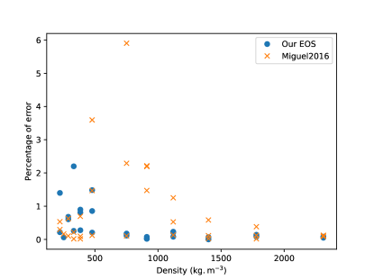
Figure 1: Relative error on the density between MH13 and our or Miguel et al., (2016) mixed EOS for Y= 0.2466 .

For the heavy elements in the H/He rich envelope, composed essentially of volatiles (H₂O, CH₄, NH₃), we use a recent EOS for water, based on QMD simulations at high density (Licari, (2016), Mazevet et al., (2018)). Here also, this EOS has been shown to adequately reproduce available Hugoniot experiments (Knudson et al.,, 2012). Given the small number fraction of CH₄ and NH₃ compared with H, He and even H₂O, we do not expect the assumption to generically treat all the volatiles with the water EOS to be consequential on the results. When considering a diluted core, we combine the above water EOS with the the Sesame ”drysand” one (Lyon and Johnson,, 1992) to take into account additional heavy elements such as silicates and iron. Finally, when including a central compact core, we use a 100% ”drysand” EOS. We verified that using e.g. an EOS for pure iron instead of the drysand one for this region does not make noticeable difference. Note that ab initio simulations have shown that, under the characteristic temperature and pressure conditions typical of Jupiter deep interior, water is in a liquid state and is fully soluble in metallic hydrogen (Wilson and Militzer, 2012b, ). Similarly, solid SiO₂ and MgO, representative examples of planetary silica and rocky material, are also found to be soluble in H⁺ under similar conditions (González-Cataldo et al., (2014), Wilson and Militzer, 2012a , Wahl et al., (2013)). These thermodynamic considerations support a core erosion for Jupiter typical central conditions and thus a mixed $H/He/Z$ eos in such a region.

As shown by Soubiran and Militzer, (2016), the inclusion of heavy elements in a H/He/Z mixture under Jupiter-like internal temperature and density conditions can be performed with the so-called Additive-Volume-Law (AVL) provided we use an effective volume (density) for the heavy species. We verified that our EOS is consistent with the work of Soubiran and Militzer, (2016), and hence that oubetween at most 0.1 and 0.3 Mbar water EOS, as representative of volatiles in Jupiter, can be used throughout the entire $T$-$P$ domain from Jupiter’s atmosphere to the center.

For H/He/Z mixtures, our EOS are then combined at each given $(P,T)$ point throughout the AVL :

$$\frac{1}{\rho}=\frac{1-Z_{\mathrm{water}}-Z_{\mathrm{drysand}}}{\rho_{\mathrm{H},\mathrm{He}}}+\frac{Z_{\mathrm{water}}}{\rho_{\mathrm{water}}}+\frac{Z_{\mathrm{drysand}}}{\rho_{\mathrm{drysand}}}\hskip 28.45274pt{\rm at}\,\,(P,T)={\rm constant},$$ (4)

where $\rho_{\mathrm{H},\mathrm{He}}$, $\rho_{\mathrm{water}}$ and $\rho_{\mathrm{drysand}}$ are the densities of the H/He mixture, water and drysand, respectively, and $Z_{\mathrm{water}}=M_{\mathrm{water}}/M$, $Z_{\mathrm{drysand}}=M_{\mathrm{drysand}}/M$ the mass fractions of water and drysand, respectively, with $M$ the mass of the planet. Note that the accuracy of the AVL for the hydrogen/water mixture under the relevant conditions for Jupiter interior has been verified with QMD simulations (Soubiran and Militzer,, 2015).

Given the small number fraction of heavy elements compared with H and He, the $P$ and $T$ used to calculate the densities in the H/He/Z mixture are the ones obtained with the H/He mixture only. Similarly, the entropy of heavy elements can be neglected (see Soubiran and Militzer, (2016)) and even when their mass fraction becomes $Z\gtrsim 0.2$, they affect the total mixing entropy by at most 2$\%$, which represents a few per thousands of the total entropy. Moreover, this occurs only in the deepest part of the planet, with little impact on the gravitational moments. Hence, the total entropy is evaluated as the entropy of a pure H-He mixture with effective hydrogen and helium mass fractions $X^{\mathrm{eff}}=X/(1-Z)$ and $Y^{\mathrm{eff}}=Y/(1-Z)$, respectively, with $X^{\mathrm{eff}}+Y^{\mathrm{eff}}=1$, and $X=M_{H}/M$, $Y=M_{He}/M$, and $Z=M_{Z}/M=Z_{\mathrm{water}}+Z_{\mathrm{drysand}}$.

2.3 Galileo constraints on the composition

For the outer element abundances, the observations of Galileo give

$$\dfrac{Y_{\rm Gal}}{(X_{\rm Gal}+Y_{\rm Gal})}=0.238\pm 0.005,\ \,$$

$$Z_{\rm Gal}=0.0167\pm 0.006,$$

where $X_{\rm Gal}$ and $Y_{\rm Gal}$ are the observed mass abundances of hydrogen and helium, respectively. $Z_{\rm Gal}$ is the abundance of heavy elements in the high envelope measured by Galileo, but the real abundance of heavy elements should be larger. This implies that $Y_{\rm Gal}$ and $X_{\rm Gal}$ are only defined relatively to each other and that $X_{\rm Gal}+Y_{\rm Gal}+Z_{\rm Gal}$ can be larger than 1. In all the following models of this paper, except if stated otherwise, we impose the external atmosphere to have helium and heavy element mass fractions:

$$Y_{\mathrm{ext}}=0.23$$

$$Z_{\mathrm{ext}}=0.02,$$

which corresponds to $Y_{\mathrm{ext}}/(X_{\mathrm{ext}}+Y_{\mathrm{ext}})=0.2347$. As just mentioned, this $Z$ value is most likely a lower limit for the heavy element content in the external envelope of Jupiter (see §5.4 for a detailed exploration of this issue). Forgetting Galileo’s constraints, i.e. reducing the observed amount of heavy elements, drastically reduces the constraints on the models and allows the derivation of a large range of models compatible with Juno’s data. Relaxing these constraints thus drastically simplifies the calculations of models consistent with only Juno’s observations. Such simplifications, as done in all recent studies (Guillot et al., (2018), Wahl et al., (2017), except when using an ad-hoc modification of their EOS), however, can hardly be justified (see §6). In all our calculations, the planet’s mean helium fraction is fixed to the protosolar value: $\bar{Y}/(\bar{X}+\bar{Y})=Y_{\odot}=0.275$ (see e.g., Anders and Grevesse, (1989)).

3 Simple benchmark models

In this section, we show that traditional homogeneous, adiabatic 2 or 3 layer interior models for Jupiter are excluded by the new observations and that the planet must consist of several different regions.

3.1 Homogeneous adiabatic gaseous envelope

We first calculate an isentropic model, composed of one homogeneous convective isentropic gaseous envelope, with $\bar{Y}=0.275$, and a spherical compact core of constant density. The total heavy material content is determined to obtain the correct mass of the planet. This model reproduces the $J_{2}$ observed value within $10^{-7}$, the maximum intrinsic precision of the CMS method (Debras and Chabrier,, 2018). The $J_{4}$ and $J_{6}$ values are compared to Juno’s ones in Figure 2 under the labels ”Isentrope”. The differences between the observed and calculated values are about $3\%$ and $6\%$, respectively, well above any numerical source of error.

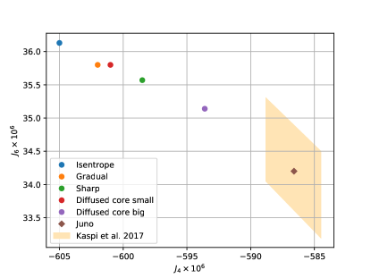
Figure 2: $J_{4}\times 10^{6}$ vs $J_{6}\times 10^{6}$ for different models (see text) and Juno’s values (Iess et al.,, 2018) with the error bars too small to be seen on this Figure. The shaded area correspond to the uncertainty on the graviational moments arising from differential rotation shallower than 10000 km, as evaluated by Kaspi et al., (2017).

The only possibility to reconcile the observed and theoretical values would be the presence of strong differential rotation affecting the calculation of the gravitational moments, not implemented in the CMS calculations. However, the results of Kaspi et al., (2017) show that with various flow profiles extending more than $10000$ km within the planet, the change in $J_{4}$ is at most $0.7\%$ (see their Figure 4). Furthermore, the study of Cao and Stevenson, (2017) excludes such a deep differential rotation.

• This yields the first robust conclusion: Jupiter’s interior is not isentropic.

3.2 A region of compositional and entropy variation within the planet

The next step in increasing complexity is to change the composition, then the entropy, somewhere in the planet. There are two physically plausible domains: a diluted core extending throughout a substantial fraction of the interior and/or a region of either layered convection, hydrogen metallisation or H/He phase separation somewhere within the envelope.

3.2.1 Two possible locations

A diluted core or a region of layered convection further up in the planet can emerge during the evolution of the planet or can be inherited from the formation process (see e.g. Stevenson, (1985), Chabrier and Baraffe, (2007) and references therein, Helled and Stevenson, (2017)) and is characterised by a compositional gradient $\nabla\mu=(\partial\mu/\partial r)\propto\nabla Z=(\partial Z/\partial r)$ with $\mu$ the mean molecular weight, thus an entropy gradient $\nabla S=(\partial S/\partial r)$. For hydrogen metallisation, 1^st-principle numerical simulations suggest it could occur through a first-order phase transition (usually denominated plasma phase transition, PPT, or liquid-liquid transition, LLT) in a domain $P_{c}\sim 1$-2 Mbar, for temperatures below the critical temperature $T\leq T_{c}\simeq 2000$-5000 K (Morales et al., (2010) , Lorenzen et al., (2011), Morales et al., 2013b , Knudson et al., (2015), Mazzola et al., (2018)). Experiments on liquid deuterium, D₂, seem to be consistent with these figures, even though significant differences still persist between various experiments (see e.g. Knudson et al., (2015), Celliers et al., (2018)). Until this issue is resolved definitively, an entropy discontinuity, $\Delta S$ due to hydrogen pressure ionisation in Jupiter’s envelope, although unlikely, can thus not be definitely excluded. In a similar vein, H/He phase separation, also a first-order transition, will also yield an entropy discontinuity, provided the local temperature is lower than the critical one for the appropriate He concentration (see below). Last but not least, a regime of double-diffusive layered convection could develop somewhere within the planet interior, triggered either by one of these two transitions (or by any phase separation involving some heavy component insoluble in metallic hydrogen) and/or simply by a local compositional gradient (Leconte and Chabrier,, 2012). Phase transitions, indeed, notably endothermic ones, are suspected of enforcing layered convection, for instance in the Earth’s mantle (Schubert et al. 1975, Christensen and Yuen, (1985)). The physical reason is the release of latent heat at the transition, which leads to thermal expansion and temperature advection which tend to hamper convection. It is interesting to note that, due essentially to the larger entropy in the plasma phase than in the molecular one, a PPT is an endothermic transition, i.e. $dP/dT<0$ along the transition critical line, according to the Clausius-Clapeyron equation, $dP/dT\propto-\Delta S/\Delta\rho$. As for the H/He immiscibility, ab initio simulations, while still differing substantially, seem to suggest a critical temperature for $x_{He}=0.08$ in the range $\sim 2000$-8000 K for $P\gtrsim 1$ Mbar (100 GPa), with a weak dependence upon pressure in the $T,P$ domain relevant for Jupiter, suggesting $dP/dT\sim 0$ for the protosolar helium value (Lorenzen et al., (2009), Morales et al., (2009), Morales et al., 2013a ) (see Fig. 13 below).

Therefore, the entropy variation in the gaseous envelope could occur either within a region of layered convection due to compositional gradients or because of either a PPT or a H/He phase separation. Needless to say, not only these three physical processes are not exclusive but they are likely to be tightly linked and thus to take place in the same more or less extended hereafter denominated ”metallization boundary region” near the Mbar.

3.2.2 Results

Following up on the above analysis, we have explored two types of models with entropy and compositional changes either in the central region (the ”diluted core”) or in the gaseous envelope, as schematically illustrated in Fig. 3. In case of a diluted core unstable to double diffusive behaviour, Moll et al., (2017) showed that a central seed could survive to erosion longer than the lifetime of Jupiter. The fact that, under Jupiter central $T$ and $P$ conditions, iron and silicates are under a solid form (see e.g., Musella et al., (2018)) tends to favor the presence of such a central seed. We thus consider the presence of a compact core at the very center of the planet. For the entropy variation within the gaseous envelope, we have considered either an abrupt ($\Delta S$) or a gradual ($\delta S$) change in entropy and composition at the metallisation boundary, between at most 0.1 and 3.0 Mbar. The obtained $J_{4}$ and $J_{6}$ values are given in Fig. 2. For the models with a change of composition in the gaseous envelope, the values for a gradual or a sharp entropy change are plotted under the labels ’Gradual’ and ’Sharp’, respectively.

In case of a gradual (continuous) change, which implies a continuous molecular H₂ to metallic H⁺ transition and no H/He phase separation, the smooth change in entropy is simply due to a composition change (see eqns. (2)-(4)). In case of a first order molecular-metallic transition, the abrupt change in entropy $\Delta S$ is used as a free parameter, discretised over a certain number of spheroids to get the proper $J$ values.

In all cases, none of these two types of models, whatever the type of change of composition and entropy, sharp or gradual, was found to be able to yield $J_{4}$ and $J_{6}$ values sufficiently close to the observed ones (labeled ’Juno’) to be explained by differential rotation or deep winds.

Another ”simple” possible interior structure model is the one suggested by Leconte and Chabrier, (2012): the entire planet would be made of alternating convective and diffusive layers. These authors, however, pointed out that this entire double-diffusive interior model could be replaced by a model with a localised double-diffusive buffer in the envelope, surrounded by large scale convective envelopes (see their §4.3), similar to the type of model explored above, which is found to be excluded. We will return to this point in §5 and 6.

This yields the following conclusions:

• Conclusion 1: The first conclusion of this section is that models of Jupiter displayed in Figure 3(a) and 3(b) cannot fulfill both Juno and Galileo observational constraints. One needs a mix of these two types of models: Jupiter is at least composed of an envelope split in two parts (an outer molecular/atomic envelope with Galileo element composition and an inner ionized one) separated by a region of compositional change, and a diluted core extending throughout a significant fraction of the planet. A compact core can also be present at the center of the planet.

• Conclusion 2: In order to decrease the values of $|J_{4}|$ and $|J_{6}|$ in the models of Figure 3, we realised that either $\Delta S$ had to be substantial (an issue explored in §5) or the heavy element content must decrease with depth in the outer part of the planet. This local decrease of $Z$ is balanced by an increase of $Y$ so that the density (and the molecular weight, see §6), of course, increases with depth. As mentioned in the introduction, one of the most stringent constraints on the models are the $Y$ and $Z$ values observed by Galileo, which are surprisingly high for the observed values of the high order gravitational moments. A local inward decrease of the metal content in some region of the planet’s gaseous envelope appears to be the favoured solution to resolve this discrepancy. This is examined in detail the next Section.

It is essential at this stage to stress the crucial role played by the H/He EOS. Using the SCvH EOS, Chabrier et al., (1992) and subsequent similar models, which fulfilled Galileo and Voyager observational constraints, could relatively easily fulfill as well the Juno ones. This is entirely due to the SCvH EOS (or, similarly, the R-EOS one (Nettelmann et al.,, 2012), see Fig. 11 of Militzer and Hubbard, (2013) or Fig. 27 of Chabrier et al., (2018)): for a given entropy, such an EOS has a lower density (pressure) in the $\sim$Mbar region than our new EOS, enabling a larger amount of heavy element repartition in Jupiter interior, relaxing appreciably the constraints on possible models. The constraints become much more stringent with stiffer, more accurate EOS’s.

Figure 3: Simple structures of Jupiter with an internal entropy variation either in the envelope (left) or in the core (right) (see §3.2.2). None of these models can match the observations of both Juno and Galileo.

4 Locally inward decreasing Z-abundance in the gaseous envelope

4.1 Inward decreasing abundance of heavy elements in some part of the outer envelope

Two physical processes can lead to a locally decreasing abundance of heavy elements with depth in Jupiter’s outer envelope, i.e. a locally positive gradient $\nabla Z>0$: a ”static” one, based on thermodynamic stability criteria, and a ”dynamic” one, which involves non-equilibrium processes. For sake of completeness, a third, more ”exotic” process, involving external events, is also discussed.

4.1.1 Thermodynamic stability

Salpeter, (1973) and Stevenson and Salpeter, 1977a (see also Stevenson, (1979)) suggested the occurence of helium differentiation in giant planet interiors, either in the same or in a different region that the H₂-H⁺ pressure metallisation of hydrogen. These authors suggested that minor constituents, namely the heavy elements, could suffer differentiation in a similar or even larger way as helium. Unfortunately, phase diagram calculations of two or more components under the typical relevant conditions for Jupiter (about 1 Mbar and 5000 K) are scarce, or even inexistent, so finding out which element, under which molar concentration, prefers the H⁺-rich or He-rich phase remains to be determined. The only existing study is the one by Wilson and Militzer, (2010). Ab initio simulations by these authors suggest that Ne association with He is thermodynamically favoured, while the opposite is true for Ar, which is found to be more soluble with H⁺. The underlying physical reason is the argon atom additional electron shell which increases its effective volume with respect to He due to the Pauli exclusion principle. If this explanation is correct, Kr and Xe should likewise be soluble in metallic hydrogen, which is consistent with their observed nondepletion in Jupiter’s atmosphere.

It is indeed intuitively appealing to think that in case some species, $Z_{i}$, is pressure ionized, it might become immiscible with neutral helium, as for H⁺/He, due to the strongly repulsive pseudo-potential, as in the case e.g. of alkali metals (Stevenson,, 1979). For some element (atom or molecule) to differentiate in the midst of some mixture, one needs its interaction energy in the mixture, typically the molecule or electron binding energy, to be larger (in absolute value) than the ideal mixing entropy, $-k_{B}\,T\ln\,x_{Z}$. Since the most abundant heavy elements have a number fraction $x_{Z}\simeq 0.1\%$, this yields near the metallization boundary, $\sim 5000$ K, $|E_{b}|\gtrsim 0.5$ eV, a condition rather easy to fulfill. As mentioned above, all heavy elements, however, do not necessarily behave similarly. Heavy noble gases, indeed, are more likely to form compounds (Hyman, (1964) Blackburn, (1966) Wilson and Militzer, (2010)), suggesting that species like neon, acting like helium, and argon, have a different behaviour in the H⁺/He mixture.

In case of element differentiation, according to the Gibbs phase rule, $x_{II}=x_{I}\exp\{-\Delta G(P,T)/k_{b}T\}$, where $x_{i}$ denotes the number abundance of a given species in phase $I$ or $II$ (H⁺-rich/poor, conversely He-poor/rich in the present context) and $\Delta G$ is the excess mixing enthalpy in the mixture, the differentiation of a given heavy element can be similar or opposite to that of helium, yielding an increasing (resp. decreasing) abundance with depth in the former (resp. latter) case. In all cases, this yields a gradient of abundance $\nabla Z$ within some part of the planet envelope, with $\nabla Z>0$ for some heavy elements.

If H-He immiscibility, leading to a depletion of helium in the outer envelope, is triggered by the metallisation of hydrogen, the fact that hydrogen metallisation in a H/He mixture is found to occur at lower pressures with decreasing helium fraction (e.g. Mazzola et al., (2018)) implies that the pressure range of immiscibility will extend with time because of both the planet’s decreasing internal temperature and the decreasing abundance (depletion) of helium in the upper layers. The region of immiscibility can thus be relatively broad in Jupiter’s interior, depending on when it started. Note in passing that, if H/He differentiation occurs and is at least partly responsible for the redistribution of heavy elements in Jupiter’s envelope, this excludes the H/He diagrams suggested by Morales et al., (2009) and Schöttler and Redmer, (2018) which predict no immiscibility within present Jupiter. This point will be discussed in detail in §6.1.

It should be stressed that, given the small number abundances of helium and heavy elements in Jupiter interior, whereas the aforedescribed demixing processes could lead to some Z-enrichment in the planet outer envelope, consistent with or even larger than Galileo’s observed value, this enrichment will remain modest and could not explain values significantly larger than $Z_{\rm Gal}$. In this latter case, external acccretion seems necessary, as examined in §4.1.3 below.

4.1.2 Upward atomic motions

As explored thoroughly by Stevenson and Salpeter, 1977a in the case of a first-order hydrogen pressure ionization (PPT) and a H/He phase separation occuring in the same region, the following process might occur. At the onset of hydrogen metallisation, characterised by a pressure $P^{+}$, latent heat release will lead to the superposition of a overheated (resp. supercooled) H⁺-rich (resp. H₂-rich) layer, thus less (resp. more) dense than the surrounding medium, underneath (resp. above) the metallization boundary (see Fig. 2 of Stevenson and Salpeter, 1977a ). Under such conditions, nucleation of bubbles might occur. Concomitantly, He atoms will differentiate from H⁺. If such H⁺-rich/He-poor bubbles form, they will absorb heat by thermal diffusivity and will be lighter than the surrounding gas. The bubbles will then rise by buoyancy, up to a pressure $P$ less than the metallisation pressure, $P<P^{+}$. They will then break and H⁺ will recombine to form H₂, depleting little by little the upper envelope in He by mixing this convective region with H⁺-rich bubbles while enriching the lower envelope in He. Consequently, the heavy elements which, for chemical and/or thermodynamic reasons, have a preference for these H⁺-rich/He-poor bubbles, rather than for the He-rich/H⁺-poor surrounding medium, will be transported upwards and be depleted little by little in the deep envelope whereas the opposite will be true for species favoring association with helium atoms. Somehow, this is similar to an ongoing distillation process in the sense that the redistribution of elements arises from a physical separation rather than a chemical reaction and mass is not locally conserved beneath the uppermost convective envelope. This occurs only if the heavy elements do not affect significantly the density of the bubbles, which must remain lighter than the surrounding gas. In the typical conditions of Jupiter’s outer envelope, there are about $500$ times more atoms of hydrogen than of heavy elements. Therefore, for a typical atomic weight ratio ${\bar{A}}_{Z}/A_{H}\sim 15/1$ (average between C, N and O atoms), such a process is possible. Heavier molecules (such as iron) being even more rare compared to H, gravitational considerations are still consistent with this scenario.

Such a scenario has further theoretical support. First, noble gases have been known to be almost insoluble in metals since the end of the 19th century (Ramsay and Travers, (1897) or Blackburn, (1966) for a review, and Wilson and Militzer, (2010) for the case of neon and argon). On the other hand, at high pressure, hydrogen can form complex polyhydrides molecules very efficiently, with many different atoms (sulfur, lithium, sodium, iron, …; see e.g. Ashcroft, (2004) or Pépin et al., (2017)). Therefore, at metallisation, non inert heavy elements tend to form polyhydrides within metallic H⁺-rich bubbles. If, as discussed above, the density of these bubbles is less than the one of the surrounding gas, these heavy elements will be transported upwards, enriching Jupiter’s outer envelope while depleting the inner one. The formation of polyhydrides, however, has been probed experimentally so far up to $\sim 1500$ K (Pépin et al.,, 2017) and remains to be explored up to $T\sim 4500K$, the onset of H metallisation in Jupiter. Further numerical or experimental work on the formation of polyhydrides at high pressures and temperatures would help assessing the validity of this process.

Concomitantly with hydrogen metallization, and the formation of polyhydrides, we also expect reduction-oxydation (redox) reactions to occur. The loss of its $1s$ electron at hydrogen metallization makes H⁺ prone to react with other heavy elements through electron transfer. The H⁺ bubbles could then trap e.g. N, O or other elements, participating also to en enrichment (resp. depletion) of these elements in the upper (resp. lower) envelope. We recall, however, that in the absence of dynamical variations such as gravity waves or upward plume penetrations, the amount of overheating due to a PPT would be insufficient to yield homogeneous nucleation (Stevenson and Salpeter, 1977a, ).

In all cases, the afore ”rising bubble” process requires hydrogen molecular-metallic transition to occur through a first-order transition, leading to a local release of latent heat. As mentioned in §3.2.1, although a PPT is indeed found in some modern ab initio numerical simulations, its critical temperature remains to be determined precisely, being predicted within the range $2000\lesssim T_{c}\lesssim 5000$ K for a critical pressure $1\lesssim P_{c}\lesssim 2$ Mbar. Interestingly enough, a critical temperature $T_{c}\simeq 5000$ K around $\sim 1$ Mbar would be consistent with a PPT in the outer part of Jupiter. In the absence of a PPT in the envelope, H⁺/He phase separation can possibly still occur but the outer observed oversolar abundance of heavy elements can not be due to upward bubble motions. Phase separation of these elements with He, as discussed in §4.1.1, will thus be the favoured explanation.

4.1.3 Accretion

Finally, the overabundance of heavy elements in Jupiter’s upper envelope can have a third explanation, namely one or several giant impacts (Iaroslavitz and Podolak,, 2007) or, similarly, ongoing accretion of planetesimals (e.g., Bézard et al., (2002)). This scenario, however, implies that global internal convective motions must be inhibited somewhere in Jupiter, preventing the extra accreted material to be redistributed homogeneously throughout the planet. Indeed, a global $Z$ abundance throughout the planet equal to the Galileo value would yield low-order gravitational moments inconsistent with observations. If convection inhibition is due to H/He immiscibility, this latter must already have started when the external event took place. This in turn puts an important constraint on the H/He phase diagram, notably on the critical $P,T$ values for $x_{He}=0.08$, Jupiter helium protosolar concentration. If inhibition is due to hydrogen metallization, it implies that this latter must be a 1^st-order phase transition (yielding an entropy jump). Convection can also be inhibited by the onset of double diffusive convection, either as an enhanced diffusive process (oscillatory convection) or as layered convection, a process possibly triggered by extensive planetesimal accretion (e.g. Stevenson, (1985), Chabrier and Baraffe, (2007) and references therein) and/or by deposition of high entropy material onto the growing planet (Berardo & Cumming 2017), preventing homogeneization of the envelope composition. In order to explain a genuine abundance significantly larger than Galileo’s observed value, $Z_{ext}\simeq 2.5\times Z_{\odot}$, the total accreted mass must be $M_{\mathrm{excess}}\lesssim 1.5\,\,{\rm M}_{\oplus}$, a significant but not unplausible value.

4.2 Constraints from the evolution

To be considered as plausible, our models with a region of locally inward decreasing abundance of heavy elements must be consistent with what is known of Jupiter’s long term evolution. If, as expected, Jupiter formed through core accretion (Pollack et al.,, 1996), the primordial abundance of heavy elements in the planet should be increasing with depth (see Fig.4). As explored by, e.g., Leconte and Chabrier, (2013), Vazan et al., (2018), the differential core-envelope cooling of the planet leads to a redistribution of heavy elements with time, yielding an increasing heavy element content in the gas rich envelope. To explain our $\nabla Z>0$, a physical process must have inhibited convection within the envelope and prevented a homogeneous redistribution of elements. Three possibilities have been discussed in the previous subsections: 1^st order metallisation, immiscibility and accretion. We examine whether they are compatible with the evolution of the planet.

If a first order metallization (PPT) stopped the convective motions, our discussion on the bubbles in §4.1.2 shows that it is possible to deplete the inner envelope and enrich the outer one. This would be in adequation with any evolutionary scenario.

In the case of hydrogen/helium immiscibility, the outer envelope will be depleted in helium because of helium sedimentation (see §4.1.1, Stevenson and Salpeter, 1977a ), yielding an enrichment in $Z=M_{Z}/M$ in this region. Note that, in order to obtain a locally steep enough gradient of heavy elements $\nabla Z>0$ between the outer, $Z$-enriched, and the inner, $Z$-depleted, envelopes, the He-rich falling dropplets must be as $Z$-poor as possible. This implies limited miscibility between some Z-components and He, in addition to H and He, and typical Z/He phase diagrams yielding very low concentations of heavy elements in He-rich dropplets, as discussed in §4.1.1. Under such conditions, it is possible to preserve (and even increase) a positive $Z$-gradient with time.

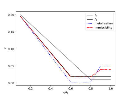
Figure 4: Typical evolution of the heavy element content $Z$ as a function of the radial distance $r$ with time, assuming that a first order phase transition (PPT) or immiscibility will occur during the cooling history. At $t=t_{0}$ Jupiter just formed. A small convective external envelope is connected to a gradually diluted planet, structure inherited from the core accretion. At $t=t_{c}$, immiscibility or first order metallisation is about to happen. The convective zone has somewhat expanded, redistributing the metal content in the planet. Later on (’metallisation’ curve), the rising bubbles have enriched the outer envelope in heavy elements while depleted the inner one. If immiscibility takes place (’immiscibility’ curve), the outer envelope will eventually lose part of its mass because of drowning helium dropplets, increasing the heavy elements mass fraction in the outer envelope whereas the dilution of these elements in the inner envelope is almost negligible.

Finally, in the absence of PPT or immiscibility, if inhibition of convection, leading to layered convection (Leconte and Chabrier, (2012)) or even partly radiative interiors during the planet’s growth, is the only reason for the difference of composition between the outer and inner envelopes, it must have persisted since the accretion event(s). Although, as examined in §6.2, the present models fulfill the constraints required for the onset and persistence of layered convection (Leconte and Chabrier, (2012), Leconte and Chabrier, (2013)), whether such structures can persist during Jupiter’s, or in fact any gaseous planet cooling history (Chabrier and Baraffe,, 2007) needs to be explored with extreme care (e.g. Rosenblum et al., (2011), Mirouh et al., (2012), Wood et al., (2013), Kurokawa and Inutsuka, (2015)) and requires that the key physical processes at play are handled with great accuracy. A fantastic challenge for numerical simulations.

To conclude this section, we should mention that recent evolutionary calculations (e.g. Vazan et al., (2018)) converge to a structure profile for present Jupiter with a monotonically outward decreasing compositional gradient, $\nabla Z<0$, at odd with our suggestion of a local $\nabla Z>0$. These models, however, use the SCvH EOS. As discussed in §3.2.2, this latter yields a too hot thermal structure along an adiabat (see Militzer and Hubbard, (2013) or Fig. 27 of Chabrier et al., (2018)), favoring convection and allowing larger metal fractions. These Jupiter internal structure models are excluded by the present Juno+Galileo analysis and thus can not be used as reliable evolutionary constraints. Further evolutionary calculations with the proper physics, including a proper treatment of double diffusive convection and of H/He phase separation are needed to verify the consistency of the present models with Jupiter’s thermal history. As just mentioned, however, properly handling such complex physical processes is a task of major difficulty (see §6.5).

5 Models with at least 4 layers and an entropy discontinuity in the gaseous envelope

As shown in §3, Jupiter interior structure must entail at least four different regions, namely two outer and inner homogeneous adiabatic envelopes, separated by a region of compositional, thus entropy variation, and a diluted core, also harboring a more or less extended domain of compositional/entropy change, and potentially a solid rocky seed. One of the unknowns in these models is the amount of entropy change in the envelope. With an entropy change only due to a change in composition (see section 2), the smallest value of $J_{4}$ we could obtain lies within the limit of what can be explained by a differential rotation shallower than $10000$ km (Kaspi et al.,, 2017). The higher order moments, however, remain much too large. This yields another conclusion:

• Models with a small entropy change in the Mbar region seem to be excluded as possible Jupiter internal structure.

Therefore, in this section the inward increase of entropy (due to H-He immiscibility or the onset of super adiabatic layered convection) is now used as a free parameter in the calculations, and is discretised throughout a certain number of spheroids across the ionization boundary region. That is we assume an entropy gradient $\nabla S=\Delta S/\Delta R<0$ within the relevant pressure range.

5.1 Physical expectations

As quickly examined in section 3.2, a brutal inward increase of $S$ can have several physical foundations. Assuming that Jupiter’s outermost thermal profile is isentropic (because of adiabatic convection in this region), the observed condition, $T=165$ K, $P=1$ bar corresponds, according to our EOS, to $T\simeq 5000$ K at 1 Mbar. As mentioned above, recent 1^st-principle simulations (Mazzola et al.,, 2018) predict a critical temperature for the metallisation of hydrogen in the range $T_{c}\simeq 2000$-5000 K at $P\simeq$ 1 Mbar. Both simulations (Soubiran et al., (2013), Mazzola et al., (2018)) and experiments (Loubeyre et al.,, 1985), however, suggest that, even for a low helium concentration as in Jupiter ($x_{He}<0.1$), the critical pressure increases while the critical temperature decreases with increasing helium concentration, which probably excludes a PPT between molecular and metallic hydrogen in Jupiter. However, given the present uncertainties in these determinations, we must still explore such a possibility.

In case of a 1st order transition, $\Delta S$ is given by the Clausius-Clapeyron relation along the critical line $P(T)$:

$$\frac{\Delta S}{\Delta(1/\rho)}=\frac{\mathrm{d}P}{\mathrm{d}T}.$$ (5)

Analytical calculations (Saumon and Chabrier,, 1992), suggest

$$\Delta S_{\mathrm{metallization}}\sim 0.5\,\mathrm{k_{\mathrm{B}}/proton}.$$ (6)

Since, as mentioned above, the temperature in this region of Jupiter’s interior should be close to $T_{c}$, we expect $\Delta S$ to be less than this value.

If hydrogen pressure ionization does not occur through a first order transition inside Jupiter, a sharp entropy change can be due to H/He phase separation (also a 1^st-order transition). As shown by Stevenson and Salpeter, 1977a , drowning nucleated helium dropplets lead to a release of gravitational energy and, even though their analysis suggest that most of this energy is radiated away, part of it contributes to heating up the inner part of the planet, raising the entropy (see detailed discussion in §6.5).

The shape of the H/He phase diagram is a major uncertainty in this context. The rather limited helium depletion w.r.t. the solar value in Jupiter’s external envelope, $x_{He}\simeq 0.1$, suggests that the variation $\Delta Y$ in the immiscible region should be modest (about $\sim 10\%$). In that case, according to Morales et al., 2013b Fig. 2, the mixing entropy should depart only slightly from the ideal mixing entropy, by $\sim 0.03\,k_{B}$/at at 5000 K for $x_{He}=0.1$. Since the maximum value of the ideal mixing entropy, for a concentration $x_{He}=0.5$ is $S_{mix}^{id}/N=-[x\ln x+(1-x)\ln(1-x)]=0.7\,k_{B}$/at (about $0.3\,k_{B}$/at for $x_{He}=0.1$), we see that the entropy jump due to H/He immiscibility should be $\lesssim 0.5\,k_{B}$/proton. The entropy change due to helium dropplet sedimentation is more difficult to evaluate and requires numerical explorations. Guidance is provided by the calculations of Fortney and Hubbard, (2003) for the case of Saturn. In the case of a maximum temperature gradient in the inhomogeneous region and no formation of a helium layer atop the core (both the most likely present situation), these authors find that a change of composition $Y=0.21\rightarrow 0.36$ corresponds to a global increase of entropy $\Delta S\sim 0.3\,k_{B}$/proton. For Jupiter, we expect helium sedimentation (i) to have occured, if ever, more recently than for Saturn, (ii) to encompass a much smaller fraction of the planet (see §6.1) and thus to induce a much smaller entropy variation. Adding up these two contributions, it seems difficult to justify an entropy jump arising from H/He phase separation much larger than:

$$\Delta S_{\mathrm{H/He}}\lesssim 1.0\,\mathrm{k_{\mathrm{B}}/proton}.$$ (7)

Clearly, more experimental and numerical exploration of hydrogen pressure metallisation and H/He phase diagram and He sedimentation process are strongly needed to help constraining these processes.

Finally, if the mean molecular weight gradient due to the change of composition is large enough to hamper adiabatic convection, a regime of layered convection can develop and lead to a super adiabatic temperature structure similar, at least in some part of the planet, to the one derived in Leconte and Chabrier, (2012). The detailed treatment of layered convection in our calculations is presented in §6.2. Varying the location and extent of layered convection between $0.1$ Mbar and $2$ Mbar, i.e. in the vicinity of hydrogen pressure ionization, we obtain numerically a maximum entropy increase from layered convection:

$$\Delta S_{\mathrm{layered}}\lesssim 0.6\,\mathrm{k_{B}/proton},$$ (8)

with a decreasing metal abundance, i.e. $\nabla Z>0$, in this region. An increasing metal abundance in this region yields higher values of $\Delta S$ but in that case $\alpha\lesssim 10^{-7}$, where $\alpha$ denotes the ratio of the size of the convective layer to the pressure scale height, $\alpha=l/H_{P}$ (see §6). This implies the presence of a diffusive buffer, or a regime of turbulent diffusion within the ionization boundary layer. Although detailed calculations are lacking, it seems difficult to reconcile such a structure with Jupiter’s thermal history.

In summary, if either a first order transition and/or layered convection is present within some part (most likely around the Mbar) of the planet gas rich envelope, an inhomogeneous zone where the total increase in entropy can reach $\sim 0.5$-$1\,\mathrm{k_{B}/proton}$ is expected.

Figure 5 portrays the typical structure of our final Jupiter models. They all share the following features:

• an outer homogeneous convective envelope characterised by the Galileo helium and heavy element abundances and the adiabat condition at $T=165$ K, $P=1$ bar;

• an inhomogeneous region between $\sim$0.1 and $\sim$2 Mbar associated with (i) a change in composition, most likely characterised by an inward decreasing metal abundance ($\nabla Z>0$) and (ii) a non negligible entropy ($\gtrsim 5\%$) and temperature increase. These gradients stem from layered convection and/or H-He immiscibility, even though a PPT can not be totally excluded for now;

• an inner homogeneous convective envelope lying on a warmer isentrope than the outer region, with an average larger helium fraction and, most likely, a lower metal fraction than in the outermost region. Indeed, even though a larger $Z$ fraction in this region than in the outer one is not entirely excluded, it requires an uncomfortably large entropy increase, $\Delta S\gtrsim 1.4\,k_{B}/$proton (case (c)), according to the aforederived estimates.

  As shown below, there is a degeneracy between the entropy jump in the inhomogeneous region and the helium and metal fractions in the inner envelope. The larger $Y$ and $Z$ in the inner envelope, the larger $\Delta S$ needs to be.

• a diluted (eroded) core extending throughout a significant fraction of the planet. A small entropy jump in the inhomogeneous region, $\Delta S\lesssim 0.5\,k_{B}/$proton (case (a)), yields an inward increasing helium abundance in the core, while a larger value (case (b)) implies an inward decreasing helium abundance in the core.

• probably, but not necessarily, a central compact, solid core.

A quantitative analysis of these models is given in the next subsection.

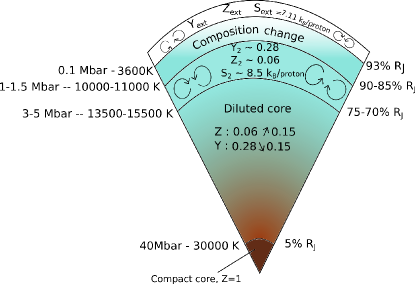
(c)

Figure 5: Schematic internal structure of our final Jupiter models. $Y_{\mathrm{ext}}=0.23$, $Z_{\mathrm{ext}}=0.02$ as stated in the text. (a) The modest entropy increase between the outer and inner envelopes yields a moderate helium increase in this latter, and an inward helium enrichment in the diluted core (see text). (b) The larger entropy increase in the inhomogeneous boudary region yields a supersolar helium fraction in the inner envelope, but then the helium abundance decreases in the diluted core. (c) Our least favoured model. An increase of both helium and heavy element abundances in the inner envelope requires a strong entropy increase, at the limit of what is physically achievable. A mixture of structures (a) and (c) is also possible, with a small increase in both helium and heavy elements. The required $\Delta S$ would be comparable to (b).

5.2 Quantitative results on the gravitational moments

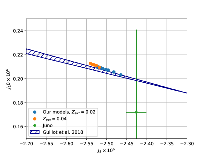
(c)

Figure 6: Gravitational moments we obtain with various models in the $J_{k}-J_{k+2}$ plans, for two values of $Z_{\rm ext}$. All the values are multiplied by $1\times 10^{6}$ as done in e.g., Guillot et al., (2018). The green dot is the Juno value with the observed error bars (Iess et al.,, 2018), without any dynamical correction. The hatched area corresponds to the models of Guillot et al., (2018).

The results of our optimized models with an entropy discontinuity $\Delta S\in[0-2]\mathrm{k_{\mathrm{B}}/proton}$ in the ionization boundary region, projected in different $J_{k}$ - $J_{k+2}$ plans, are displayed in Figure 6 for two values of external heavy element abundance, namely $Z_{\rm ext}=Z_{\odot}$ and $Z_{\rm ext}=2\times Z_{\odot}$. The first obvious conclusion from this figure is that our range of models consistent with Juno’s observed gravitational moments differs from the one derived by Guillot et al., (2018) with 200 000 models (see their Fig. 1 of the Extended Data, reported as a hashed area in Fig. 6). We have verified that this is not a discretisation issue: with interior structures calculated with 1000 spheroids, this conclusion is unaltered. Even though the difference between the two analysis should partly stem from the different EOS used by these authors, it arises essentially from our different representation of the planet interior. Indeed, we recall that these authors do not take into account the constraint from Galileo on the heavy element abundances. Therefore, if Galileo’s observations are correct, Fig. 6 shows that the qualitative conclusions these authors draw about differential rotation could be altered.

- Impact on the low-order moments ($\leq J_{4}$). We found out that the entropy change, $\Delta S$, is strongly affected by the composition in the inner convective envelope, i.e. the region between the inhomogeneous one and the diluted core. Therefore the size and composition of the diluted core, the composition of the inner envelope, and the entropy change $\Delta S$ in the region of compositional variation are intrinsically linked. To better understand this result, we must recall that the major issue of the models is to decrease $J_{4}$ at constant $J_{2}$. Figure 7(a) portrays the value of the contribution function $J_{2}-J_{4}$ in the planet as a function of pressure.

Figure 7: (a) Subtraction of the contribution functions for $J_{2}$ minus $J_{4}$, both normalized to their maxima, with respect to pressure or radius, for an isentropic model. (b) Normalized difference of contribution functions for $J_{2}$ to $J_{8}$ between a model with a small entropy change and a model with a strong entropy change.

This figure shows that, in order to decrease $J_{4}$ with respect to $J_{2}$, one needs to enrich the planet deeper than $\sim 2\,\mathrm{Mbar}$, and the region around $\sim 10\,\mathrm{Mbar}$ is where it is most efficient. Therefore, an enriched inner envelope decreases $J_{4}$ at constant $J_{2}$ (see the pressure range in Figure 7(a)); but enriching the inner envelope implies a steeper compositional gradient in the boundary region between the outer and inner envelopes, which has the opposite effect on $J_{4}$ compared to $J_{2}$. Furthermore, this boundary region between $\sim$0.1 and 2 Mbar has a much stronger contribution on $J_{2}$ and $J_{4}$ than the deeper region. This stems from the fact that this region has a high mean radius, hence the mass of a spherical shell is much larger than in the 5 Mbar region, and the impact on $J_{2}$ and $J_{4}$ is enhanced. In consequence, a small change in the $\sim 0.1-1$ Mbar region must be compensated by a strong change in the diluted core.

- Impact on the high-order moments ($>J_{4}$). The high order gravitational moments strongly depend on the value of $J_{4}$, as shown by Guillot et al., (2018). For a given $J_{4}$, the other parameters affecting these moments are the external abundance of metals (as expected), and the mass of the central compact core. Changing the helium content within the inner convective envelope has almost no impact, as there is a trade-off between the inner abundances of helium and heavy elements and the entropy increase, without affecting the high order gravitational moments. Similarly, the position and extent of the boundary region of compositional change is a second order correction to the $J_{6}$ to $J_{10}$ values. As a whole, we found out that the $J_{6}$ to $J_{10}$ values are not much affected by the composition in the inner part of Jupiter, deeper than where the compositional change occurs.

As mentioned above, we found out that some models with an inward increase of heavy elements in the envelope inhomogeneous region ($\nabla Z<0$) can fulfill all observational constraints (case (c)) provided the entropy change around $\sim 1$ Mbar reaches values $\Delta S>1k_{\mathrm{B}}/\mathrm{proton}$. This requires a strong entropy discontinuity induced either by a PPT for $T\simeq 4500$ K (thus a critical point $T_{c}\gg 4500$ K) or by H/He differentiation and sedimentation, as layered convection alone cannot yield such an entropy jump. Therefore, although not entirely excluded, models with $\nabla Z<0$ throughout the entire envelope are rather uncomfortable, as discussed in §5.1. In contrast, models with an inward decreasing abundance of heavy elements ($\nabla Z>0$) in this region require a more modest entropy change.

The fact that, surprisingly, the mass of the compact core affects the high order moments can be explained as follows. Since we consider the central compact core as spherical, it has no direct influence on the gravitational moments. However, in that case, a smaller fraction of the planet’s mass is available to satisfy the $J$ values. Since the outer envelope composition is constrained by Galileo, one can only enrich the inner envelope or the diluted core to compensate. Fig. 7(a), however, shows that if there is a too large increase of density deeper than $2$ Mbar, the increase of $J_{2}$ is larger than the one of $J_{4}$ (and even larger than the increase of the higher order moments, not shown). This leads to

$\bullet$ Conclusion 1: for given $J_{2}$, a central compact core tends to decrease the moments of order $\geq J_{4}$ compared to a model with only a diluted core.

Increasing the mass of the compact core thus implies to add more heavy elements in the inner regions of the planets, diluted core or inner envelope to reproduce the $J$ values. But the larger the amount of heavy elements in the deep layers the larger the required entropy jump $\Delta S$ between the outer and inner envelopes. This, in turn, has consequences on the high order moments: a model with a high $\Delta S$ in the metallisation region implies a higher temperature, and thus a lower density for a given composition at given pressure in the Mbar region than a model with a smaller $\Delta S$. The lower density means that this region has a smaller contribution to the gravitational moments than in the case of a small $\Delta S$. Although, for $J_{2}$ and $J_{4}$, this can be balanced by a higher contribution of the internal layers (deeper than a few Mbars), this is not the case for the higher order moments.

To illustrate this result, we show in Figure 7(b) the differences $\Delta J_{n}$ in the contribution functions $J_{2}$ to $J_{8}$ between a model with a small entropy change, $\delta S<0.1\,\mathrm{k_{\mathrm{B}}/\mathrm{proton}}$, in the ionization boundary region, only due to a composition change, and a model with a total entropy discontinuity $\Delta S=0.9\,\mathrm{k_{\mathrm{B}}/\mathrm{proton}}$. We see that the region of the outer (molecular) envelope has always a stronger contribution to the $J$’s when the entropy change is small, as expected, whatever the order of the moment. On the other hand, the inner region of the diluted core has much more impact on $J_{2}$ than on the other moments. A strong $\Delta S$ thus requires more heavy elements in the diluted core to preserve $J_{2}$ while the high order moments are almost insensitive to the enhanced composition in the diluted core. This leads to

$\bullet$ Conclusion 2: an entropy jump in the envelope tends to decrease the value of the high order moments at a given $J_{2}$. And a large enough entropy change is necessary to preserve the correct balance between the moments.

As discussed in §5.1, however, the possible entropy increase in the metallization boundary region is limited by physics principles. For central compact cores larger than $\gtrsim 5\,{\rm M}_{\oplus}$, one needs $\Delta S>1\,\mathrm{k_{\mathrm{B}}/\mathrm{proton}}$, which, as discussed above, seems to be hardly possible at these temperatures. Figure 8 displays the values of the high order gravitational moments as a function of the entropy jump $\Delta S$. Small (absolute) values of $J_{6}$, $J_{8}$ or $J_{10}$ allways require a significant $\Delta S$, except if we decrease the atmospheric $Z_{\rm ext}$, violating in that case Galileo’s constraint, as done in all recent studies. Models with no entropy jump in the gaseous envelope thus seem to be excluded, as mentioned previously.

As seen in Fig. 8, none of our models can match the $3\sigma$ error bars on $J_{6}$ for $\Delta S<1\,\mathrm{k_{\mathrm{B}}/proton}$ when considering the contribution from the winds derived in Kaspi et al., (2018). This is particularly true if the external abundance of heavy elements $Z_{\mathrm{ext}}$ is supersolar (see §5.4). When considering the dynamical correction from Kaspi et al., (2017), however, flows extending down to $3000$ km are sufficient to explain the discrepancy with the observed gravitational moments. Therefore, either the $\Delta J_{6}$ correction due to the wind contribution in Kaspi et al., (2018) is underestimated, because of an erroneous estimation of the winds or the presence of North-South symmetric zonal flows which will affect the even gravitational moments, or the entropy increase must reach at least $\sim 1.5\,\mathrm{k_{\mathrm{B}}/proton}$. In any case, a continuously increasing heavy element mass fraction with depth, i.e. $\nabla Z<0$, in the Mbar region is hard to justify (on Fig. 8, such models all have $\Delta S\gtrsim 1\mathrm{k_{\mathrm{B}}/proton}$).

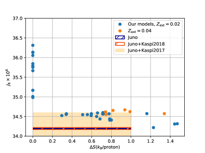
(a)

Figure 8: High order gravitational moments as a function of the entropy jump $\Delta S$ in the envelope. All these models have $J_{2}$ and $J_{4}$ values within the allowed range from Juno’s observations with the Kaspi et al., (2018) correction , except those with $\Delta S=0$ for which we could not even match $J_{4}$. The $Z_{ext}$ value is the atmospheric $Z$, ’Juno’ corresponds to the observations of Juno with the $3\sigma$ error bars, ’Juno + Kaspi2018’ are the observations corrected by the winds estimated in Kaspi et al., (2018), and ’Juno + Kaspi2017’ includes the correction to the observed gravitational moments due to a differential rotation shallower than 3000 km, from Kaspi et al., (2017). While several models are compatible with Juno’s observations when taking into account the corrections due to differential estimated by Kaspi et al., (2017), this becomes much more difficult when considering the correction derived from the odd gravitational moments by Kaspi et al., (2018). Note that, in this latter case, none of the models with $\Delta S=0$ or $\nabla Z<0$ can reproduce the gravitational moments of Jupiter.

As shown in Fig. 5, the valid models predict a size for the metallization boundary region, $l_{b}\approx 15\%$ of Jupiter’s radius. Clearly, this is orders of magnitude larger than any possible interface due to a PPT. It can, however, be consistent with the size of the inhomogeneous H/He region, as this latter keeps expanding during the planet’s cooling. Finally, as shown in §6.2, this region, characterised by a compositional gradient, is prone to layered convection, by itself characterised by a superadiabaticity and thus by its own entropy variation, to be added up to the one issued from a phase transition, and thus contributing to the total $\Delta S$.

5.3 Optimized Jupiter models

Figure 9 portrays the thermodynamic and composition profiles of our models consistent with all Galileo and Juno constraints, taking into account for this latter the correction due to differential rotation from Kaspi et al., (2017) and Kaspi et al., (2018), respectively. Profiles for an isentropic interior structure, inconsistent of course with the observed gravitational moments, are shown for comparison. The blue curves represent our favoured models, with $J_{6}$ compatible with Kaspi et al., (2017) but not with Kaspi et al., (2018) while the red curves are the profiles obtained from a model with a lower $J_{6}$, at the limit of what can be reached according to Kaspi et al., (2018). Globally, the pressure and density profiles differ by a few percents at most from the ones of the isentropic model, barely visible on the figure. However, it is worth stressing that the density of the optimized model is smaller in the Mbar region than the one of the isentropic model whereas the opposite is true in the central regions (diluted and compact core). This is a direct consequence of the constraints arising from the gravitational moments and the Galileo observations, as it allows to decrease the $J_{4}$ to $J_{10}$ values for the correct $J_{2}$. In contrast, the temperature departs from the isentropic profile for $R\lesssim 0.9\times R_{J}$, i.e. within most of the interior, by a difference $\Delta T\simeq+1000$-2000 K. Interestingly enough, this temperature increase agrees very well with the value obtained by Fortney and Hubbard, (2003) in the H/He inhomogeneous layer for a helium enrichment in the interior from $Y=Y_{\odot}$ to $Y=0.35$, and a temperature gradient leading to overstable convection. As a consequence, the specific entropy increases from the outer to the inner envelope. This increase is steeper for the model with a lowered $J_{6}$ (consistent with Kaspi et al., (2018)). For this latter, the inner isentropic envelope occupies a very limited fraction of the planet, $0.89\times R_{J}\lesssim R\lesssim 0.92\times R_{J}$, and the diluted core extends up to 85% of the planet. Within the diluted core, the specific entropy decreases drastically due to the strong increase in heavy elements (Figure 9(b)). We do not show the specific entropy and compositional profiles in the diluted core because of the degeneracy between helium and heavy element distributions in this region, which yield similar results for the gravitational moments. Let aside the fact that the entropy profile is of no real interest in this region. The important parameter is the steepness of the gradient of composition between the inner envelope and the diluted core. The steeper the gradient, the smaller the diluted core needs to be to obtain the correct $J_{2}$. The mean heavy element mass fraction is displayed in Fig. 9(b). As discussed earlier, $Z$ is decreasing between the outer and inner envelopes ($\nabla Z>0$), as models with a continuously increasing $Z$ ($\nabla Z<0$) in the envelope, although not strictly excluded, require a very large entropy jump ($\Delta S>1k_{\mathrm{B}}/$proton), difficult to reconcile with the examined physical processes (§5.2.1). Future work in this direction will certainly help clarifying this issue.

Figure 9: (a) Pressure, temperature, density and specific entropy as a function of radius for an isentropic (dashed gray) structure of Jupiter, a model with a high $J_{6}$ value (blue), compatible with Kaspi et al., (2017), and a model with a lowered $J_{6}$ compatible with Kaspi et al., (2018) (red). (b) Hydrogen (X), helium (Y) and heavy element (Z) mass abundances for the same models. The black crosses correspond to $P=1\mathrm{Mbar}$, about the region of hydrogen pressure dissociation/ionization. The outer and inner convective zones correspond to the regions of constant (homogeneous) composition and entropy, whereas the gradients are representative of the envelope inhomogeneous region and the outer part of the diluted core, respectively.

Figure 10: (a) Normalized mass as a function of radius for a model matching observational constraints and an isentropic model. (b) Mass of heavy elements (in Earth masses) as a function of radius for the same models.

Figure 10a portrays the corresponding mass profile of our typical optimized Jupiter interior structure fulfilling Juno and Galileo constraints with the wind correction of Kaspi et al., 2017. An isentropic profile is shown for comparison. The black circle indicates the inner limit of the outer convective zone while the two crosses bracket the inner convective zone and the diamond corresponds to the limit of the compact core if present. The zoom on the right hand side shows the inner convective zone, encompassing about $30\%$ of the mass of the planet. The heavy element distribution is displayed in Fig. 10b. For models with no central compact core, the total amount of heavy elements in the planet is $M_{Z}=25$-30 M_⊕. Adding up a compact core yields up to $M_{Z}=40$-45 M_⊕.

5.4 Supersolar atmospheric abundance of heavy elements

As discussed in §3, we have taken a very conservative lower limit for the true average metal content in the atmosphere, $Z_{\rm ext}$, in our calculations. We have taken a solar value, while Galileo measured abundances of individual heavy elements, excluding oxygen and neon, rather yield $Z_{\rm Gal}^{true}\approx(2-3)\times Z_{\odot}\approx 0.04$-0.06. Interestingly, such a highly oversolar value seems to be supported even for oxygen by the latest observations of the great red spot (Bjoraker et al.,, 2018). Increasing $Z_{\rm ext}$ for a given structure increases $|J_{6}|$ to $|J_{10}|$ and thus implies either a very strong differential rotation or a very large $\Delta S$ to preserve the moments. If $Z_{\rm ext}\simeq 0.05$, models with a constant inward increase of $Z$ in the metallization boundary region lead to a $\Delta S$ much larger than the aforederived 1 $k_{B}/\mathrm{proton}$ maximum value consistent with physical estimates. This reinforces our previous conclusion:

• Jupiter internal structures with an inward increase of heavy elements within the Mbar boundary region imply uncomfortable physical constraints: the entropy jump or amount of differential rotation required to be compatible with the high order gravitational moments need to be very large. In contrast, models with a locally decreasing abundance of heavy element within Jupiter’s metallization boundary region fulfill all constraints with acceptable levels of entropy variation and differential rotation.

The $J$-values for five models with $Z_{\rm ext}>Z_{\odot}$ are shown in Fig. 8 (orange circles). We see that, for a given $\Delta S$, these models have higher $|J_{6}|$ to $|J_{10}|$ values than models with $Z_{\rm ext}=Z_{\odot}$. Although some of these models are compatible with the correction due to differential rotation estimated in Kaspi et al., (2017), they are hardly compatible with the observations when considering the correction to the even gravitational moments estimated in Kaspi et al., (2018). We recall, however, that all the models of Figure 8 have $J_{2}$ and $J_{4}$ values consistent with Kaspi et al., (2018). Because of the strong correlation between $J_{4}$ and $J_{6}$, further decreasing $|J_{4}|$, consistent then with Kaspi et al., (2017) but not with Kaspi et al., (2018), would allow us to decrease the $|J_{6}|$ and higher order moment values, expanding the range of plausible models. The derivation of precise constraints on the depth penetration of differential rotation and its effect on the $J$’s as a function of $Z_{\rm ext}$ will be examined in a subsequent paper.

6 Discussion

In this section, we examine in details the reliability of the various assumptions used in the models.

6.1 Hydrogen pressure metallization and H/He phase separation

First, following the nomenclature of Stevenson and Salpeter, 1977a , we have assumed that Jupiter had a ”hot start”, meaning that the initial inner temperature of the planet was higher than the critical temperature of both hydrogen metallization through a PPT, $T_{c}(H-H_{2})$, and H/He demixion, $T_{c}(H-He)$ (for $x_{He}=0.08$). According to all existing numerical simulations aimed at exploring these issues, this is quite a safe assumption. Further work on the metallisation of hydrogen and the H/He phase diagram will enable us to discriminate between the sectors I, II and III of Figure 1 of these authors, namely:

• Sector I : if $T_{c}(H-H_{2})<T(P)<T_{c}(H-He)$, where $T(P)$ is the local temperature at pressure $P$, hydrogen metallisation is occuring smoothly but probably triggers H/He or Z_i/He immiscibility. The only possibility to deplete (resp. enrich) the inner (resp. outer) envelope in metals is to invoke 2-body or 3-body immiscibility diagrams between partially pressure ionized heavy elements $Z^{n+}$ and neutral He, similar to what is occuring for H⁺-He phase separation, as explored in §4.1.1, and/or external accretion events, depending on the exact value of $Z_{\rm ext}$.

• Sector II : $T_{c}(H-H_{2})\sim T_{c}(H-He)$. As for the Sector I case, an inhomogeneous region forms which is depleted in He and some Z-components, but in that case there is a possibly of H⁺-rich bubble nucleation and thus uplifting He-poor, Z-rich bubbles and dropping He-rich dropplets (§4.1.2).

• Sector III : if $T_{c}(H-H_{2})>T_{c}(H-He)$, H/He demixion has not started yet, the redistribution is due to the aforementioned H⁺-rich, He-poor bubbles. This is probably the most unlikely situation.

These situations are imposed by the necessity to globally increase the metal content of the upper envelope (and conversely deplete the lower one) to fulfill Galileo’s constraints, $Z_{\rm ext}\geq Z_{\rm Gal}$, but also to enrich the inner helium content, $Y$, to balance the $Z$ decrease. According to current work on metallisation and immiscibility of hydrogen and helium, even though substantial uncertainty remains, and if, as found in numerical simulations, hydrogen (or any heavy component) ionization triggers immiscibility with He atoms (or He-like ones), the Sector I case is the most likely one. This urges the need for numerical explorations of this type of diagram and, more generally, of the stability of H/He/Z mixtures under Jupiter internal conditions.

Noticeable differences still exist between modern ab-initio calculations aimed at characterising the H/He phase diagram. Figure 11 portrays the immiscibility region predicted by some of these calculations with the $T$-$P$ profiles obtained with our favoured models fulfilling all Galileo and Juno constraints, taking into account either the Kaspi et al., (2018) (low $J_{6}$) or Kaspi et al., (2017) (high $J_{6}$) correction due to differential rotation. Figure 11(a) corresponds to interior structures with strongly superadiabatic layered convection occuring at $P\geq 0.1$ Mbar. Figure 11(b) displays two models (labeled ’Morales’ and ’Lorenzen’, respectively) for which the change of entropy is only due to the H/He phase separation, i.e. occurs at the corresponding critical pressures, without any layered convection above this layer. A Jupiter isentropic profile is shown for comparison. As seen in the figure, while, according to the Lorenzen et al., (2009) calculations, H/He phase separation could take place in some fraction of our favoured Jupiter interior models, it is not the case with the results of Morales et al., 2013b (or Schöttler and Redmer, (2018), not shown) which predict no H/He immiscibility in present Jupiter. For the models with no layered convection above the phase separation (dash dotted lines in Fig. 11(b)), the temperature gradient is probably too high for overstable modes to persist, and convection will prevail (see e.g., Figure 3 of Stevenson and Salpeter, 1977a ). Although the lack of excess (non-ideal) mixing entropy in Lorenzen et al., (2009) calculations casts doubt on the reliability of their phase diagram, it is worth noting that a $\sim 200$-800 K underestimation of the critical temperature in the 1-2 Mbar domain by Morales et al., 2013b (no temperature error bar is shown in these calculations) would be consistent with immisciblity for our model with $Y_{2}=0.25$. Therefore, Jupiter’s present internal structure could entail a region of layered convection starting around $\sim 0.1$ Mbar, associated with some change in composition, and a (probably small) region of H/He (most likely H/He/Z) immiscibility at deeper levels. Although more numerical exploration of this major issue is certainly needed, key diagnostics on H/He phase separation under the relevant conditions might be provided by existing experiments (Soubiran et al.,, 2013).

Figure 11: Temperature-pressure profiles of different Jupiter models, overplotted on the immiscibility diagrams of Lorenzen et al., (2009) (pale yellow area) and Morales et al., 2013b ( orange area). All models (except isentrope) have $J_{2}$ and $J_{4}$ matching the Juno values corrected by the estimated differential rotation of Kaspi et al., (2018), and a mass abundance of heavy elements in the inner envelope $Z_{2}=0.005$. The $Y_{2}$ value is the mass abundance of helium in the inner envelope, as in Figure 5. ’Isentrope’: fully isentropic structure, with $Y=0.275$. ’High $J_{6}$’: models with $J_{6}$ compatible with Kaspi et al., (2017) but not Kaspi et al., (2018). ’Low $J_{6}$’: model with $J_{6}$ compatible with Kaspi et al., (2018). This latter model seems difficult to justify physically (se text). (a) Models with layered convection fo $P\geq 0.1$ Mbar. (b) The ’Morales’ and ’Lorenzen’ profiles are isentropic up to the onset of immiscibility according to the two related phase diagrams (see text).

As seen in Figure 11, it seems difficult to reconcile a H/He phase separation, according to the most recent calculations, with a model reproducing the Kaspi et al., (2018) $J_{6}$ value. Furthermore, the required entropy increase for this model leads to such a steep temperature gradient that unstable convection will prevail. It is thus very difficult to justify the very large entropy change $\Delta S$ in Jupiter’s gaseous envelope required in this model on physical grounds. This suggests either a revision of the Kaspi et al., (2018) analysis, or the presence of North-South symmetric winds which are inconsequential for the odd gravitational moments, but would increase the correction to the even gravitational moments, rejoining the corrections obtained in Kaspi et al., (2017).

6.2 Layered convection

As found out in the previous sections, fulfilling both Galileo and Juno constraints, while preserving a global mean helium protosolar value $\bar{Y}=Y_{\odot}$ and a physically acceptable entropy increase $\Delta S$ in the hydrogen metallization region requires an inward decrease of heavy element abundance in this region, i.e. a locally positive gradient, $\nabla Z>0$. We verified that, because of the $\sim 1/40$ heavy element to helium number ratio, this region still exhibits a positive molecular weight gradient, $\nabla_{\mu}=(d\log\mu/d\log P)>0$. In that case, large scale adiabatic convection can be inhibited and lead to a regime of small scale, superadiabatic double diffusive convection (also called semi-convection) to transport heat. As mentioned previously, although a first order transition is not required to trigger such a process, it strongly favors it, as suggested for instance at the Earth’s mantle boundary (e.g. Christensen and Yuen, (1985)).

The condition for the onset of double diffusive convection reads (e.g., Stern, (1960)):

$$0<\nabla_{T}-\nabla_{\mathrm{ad}}<\frac{\alpha_{\mu}}{\alpha_{T}}\nabla_{\mu},$$ (9)

where $(\alpha_{\mu}=(\partial\mathrm{ln}\rho/\partial\mathrm{ln}\mu)_{P,T}$ and $\alpha_{T}=(\partial\mathrm{ln}\rho/\partial\mathrm{ln}T)_{P,\mu}$. In geophysics, it is well known that double-diffusive convection generally takes the form of oscillatory convection or layered convection, i.e. a stack of small-scale convective layers of size $l$ separated by diffusive interfaces (e.g., Rosenblum et al., (2011)). In astrophysical objects, because essentially of the lower Prandtl number, this layering is more blurred and, according to simulations, double-diffusive convection rather takes the form of ill-defined turbulent interfaces, even though finite amplitude layering remains a possibility (Moll et al.,, 2016). In the absence of simulations in the present context, we will use the analytical formalism derived by Leconte and Chabrier, (2012) to verify the presence of layered convection in our models. As shown by these authors, this is controlled by the parameter $\alpha$, which is the ratio of the size of the convective layer to the pressure scale height, $\alpha=l/H_{P}$. From their eqn.(21), we can relate this parameter to the superadiabatic gradient, $(<\nabla_{\mathrm{T}}>-\nabla_{\mathrm{ad}})$, by:

$$<\nabla_{\mathrm{T}}>-\nabla_{\mathrm{ad}}=\epsilon_{d}\times\Bigl{[}(\Phi_{0}\alpha^{4}\epsilon_{d})^{\frac{-1}{4(1+a)}}+(\Phi_{0}\alpha^{4}\epsilon_{d})^{\frac{-a}{(1+a)}}\Bigr{]},$$ (10)

with layered convection occuring when

$$10^{-9}-10^{-6}\lesssim\alpha\lesssim 10^{-4}-10^{-2},$$ (11)

with, for Jupiter, the lower bound being more likely $10^{-5}$ (see Table 1 of Leconte and Chabrier, (2012)).

As MacLaurin spheroids have by definition a constant density, layered convection cannot be prescribed very accurately with the CMS method. As for the case of a first order phase transition/separation, we have implemented a sharp entropy and composition change at constant $T$ and $P$ between consecutive layers. We can then verify, for the appropriate models, whether conditions (11) and (9) are fulfilled or not. Figure 12a displays the values of $(\alpha_{\mu}/\alpha_{T})$, calculated with our EOS, for an isentropic profile and for two profiles with an entropy increase in the Mbar region of $0.5$ and $1\,\mathrm{k_{\mathrm{B}}/proton}$, respectively. We see that this quantity increases with depth by an order of magnitude, between $\alpha_{\mu}/\alpha_{T}=1$ in the external layers and the values prevailing at depth in Jupiter, due essentially to the onset of of H₂ dissociation (see Chabrier et al., (2018)). This favors the onset of layered convection deeper than $\sim 0.1$ Mbar (see eqn.(9)). Figure 12b displays the values of $\alpha$ and of the parameter $R_{\rho}^{-1}=(\alpha_{\mu}/\alpha_{T})\nabla_{\mu}/(\nabla_{T}-\nabla_{\mathrm{ad}})$ (overstable convection occurs for $R_{\rho}^{-1}>1$, see Rosenblum et al., (2011), Mirouh et al., (2012), Leconte and Chabrier, (2012)), for a composition change from ($Y_{ext}=0.23\ ,Z_{\rm ext}=0.03$) to ($Y_{2}=0.3\ ,\ Z_{2}=0.01$), with an entropy increase $\Delta S=0.45\,\mathrm{k_{\mathrm{B}}/proton}$ between $0.1$ and $1$ Mbar. We see that $\alpha$ and $R_{\rho}^{-1}$ fulfill the conditions for the presence of layered convection in this domain. Models with higher $\Delta S$ (of at most $\sim 0.6\,\mathrm{k_{\mathrm{B}}/proton}$, see §5.1) require larger $\Delta Y$. Globally, we verified that all our favoured models do fulfill the conditions for the occurence of layered convection derived in Leconte and Chabrier, (2012).

One word of caution should be noted: when H₂ dissociates into atomic H⁺, the mean molecular weight $\mu$ decreases brutally. According e.g. to Nellis et al., (1995), however, the fraction of dissociation is about $10\%$ at $1.4$ Mbar. The molecular weight thus remains barely affected up to this pressure and the decrease of $\mu$ do to H₂ dissociation should happen over a rather limited region between $\sim 1.4$ and $2$ Mbar. Whether layered convection is still present or not in this domain is less clear (although overshoot probably occurs) but we consider it to be localized enough to not significantly modify the aforecalculated temperature profile.

Figure 12: (a) $\alpha_{\mu}/\alpha_{T}$ as a function of pressure for an isentropic model and two models with $\Delta S=$ $0.5$ and $1\,\mathrm{k_{\mathrm{B}}/proton}$, respectively. (b) $\alpha$ (eq.11) and $R_{\rho}^{-1}$ (see Leconte and Chabrier, (2012)) for the model described in the text.

6.3 External impacts, atmospheric dynamical effects

We examine here whether Galileo’s high heavy element abundances in the outermost part of the envelope could be due to recent impact or recently accreted material which would not have had time yet to be redistributed within the planet and thus would not affect its gravitational potential. In that case, Juno’s contraints could be examined without taking into account the ones from Galileo. Using standard equations of the mixing length theory (Kippenhahn and Weigert, (1990), Hansen and Kawaler, (1994)), the typical convective velocity in Jupiter scales as:

$$v_{\mathrm{conv}}\approx 10\,({\nabla-\nabla_{ad}\over 10^{-8}})^{1/2}({H_{P}\over 10^{6}\,{\rm m}})\,\,{\rm m}\,{\rm s}^{-1},$$ (12)

with $(\nabla-\nabla_{ad})$ ranging from $\sim 10^{-10}$ at the center to $\sim 10^{-6}$ near the surface, yielding $v_{\mathrm{conv}}\sim$ a few to about $\sim 100$ cm s^-1 from the center to the surface.

This means that, within at most a few years, the external extra material will be mixed throughout most of the planet. It is quite clear that Jupiter has not accreted a few Earth masses of heavy elements in the past 20 years. The only source of uncertainty is Shoemaker-Levy 9. Although its mass is ridiculously small compared to the mass of the envelope, and even to the mass of heavy elements in the envelope of Jupiter, the energy deposited when it crashed onto the planet (end of July 1994) triggered uplifting of deep material (e.g, Bézard et al., 2002 or Moreno et al., 2003). As Galileo entered Jupiter’s atmosphere 1.5 year later (7 December, 1995), the material had probably be mixed again throughout the upper envelope (remember $v_{\mathrm{conv}}\approx$ 1 $\mathrm{m\,s}^{-1}$ in this region). Therefore, taking into account Galileo’s observations of Jupiter’s heavy element external abundance seems to be mandatory when trying to recover Juno’s gravitational moments.

Atmospheric dynamical effects (for instance a vortex), on the other hand, could have produced a localised maximum concentration of heavy material, not representative of the (lower) average value. Additional information is provided by the Juno microwave instrument (Li et al.,, 2017) that suggests a rather unexpected amonia vertical profile. However, if we compare the Fig. 4 of these authors with the location where the Galileo entry probe dived (around 5-10^∘ in planetocentric latitude), we see that, compared to the region deeper than $100\,\mathrm{bar}$, Galileo can have only measured a lower limit of the amonia content. Indeed, there seems to be a maximum of amonia concentration in the equatorial regions, followed by a minimum in the mid latitudes. Galileo entry probe dived at the limit between these two regions, and, most importantly, the concentration anywhere above the $25$ bar level is smaller than the one deeper than $100$ bars, where convective mixing definitely takes place. Therefore it seems unlikely that the measurements of Galileo, consistent with an increase of ammonia with depth up to $25$ bars, are an upper bound of the heavy element composition.

One can also wonder whether the composition varies between the $P=1$ bar and $P=100\,\mathrm{bar}$ levels, affecting the gravitational moments, and then should be parametrized instead of being assumed to be constant. Between two models with $(Y,Z)=(0.23,0.02)$ and $(Y,Z)=(0.23,0.04)$ in the external envelope, we get changes in $J_{2}$ and $J_{4}$, due to the first 100 bar variation, of at most $2\times 10^{-6}$ and $2\times 10^{-7}$, respectively, about an order of magnitude smaller than the change due to differential rotation (Fig. 3 of Kaspi et al., (2017)). Variations of composition in the external envelope are thus a second order correction compared to differential rotation.

6.4 Magnetic field

Although the magnetic field at the surface of Jupiter has been shown to vary with latitude and longitude within an order of magnitude (Connerney et al.,, 2018), the leading feature is a dipolar field with moment $M=4.170\times 10^{-4}\,\mathrm{T}$. According to numerical simulations, self consistent dynamo action is generally found to start when the convective magnetic Reynolds number, i.e. the ratio of magnetic field production to Ohmic dissipation, $Rm=v_{rms}d/\eta$, where $v_{rms},d$ and $\eta$ denote respectively the rms flow velocity, the thickness of the shell and the magnetic diffusivity, exceeds a critical value $Rm\gtrsim 50$ (Christensen and Aubert,, 2006). Using simple scaling arguments (e.g. Chabrier et al., (2007) and §6.3), it is easily verified that this condition is well fulfilled at the ionization boundary, located around $P\approx 1\,\mathrm{Mbar}$, where the density is $\rho\approx 800\,\mathrm{kg\,m}^{-3}$, radius $R\approx 0.85\times R_{\mathrm{J}}$, and that deeper in Jupiter convective, metallic zone we get $Rm\gg 10^{5}$. This suggests that the primary dipole-dominated magnetic field is created at depth where $Rm$ is significant, the electrical conductivity high, and the density contrast relatively mild. This is indeed what is found in state-of-the-art numerical simulations which reveal that the combination of a deep-seated dipolar dynamo and a magnetic banding associated with the equatorial jet reproduce Jupiter field geometry with realistic relative axial dipole, equatorial dipole, quadrupole and octupole field contributions (Gastine et al.,, 2014). These simulations are also consistent with the suggestion that the mean internal field strength as well as the mean convective velocity scale with the available convective power (Christensen and Aubert,, 2006). Gastine et al., (2014) find that Jupiter’s surface magnetic field strength, $B_{J}\simeq 7$ G, is consistent with a typical rms flow velocity $\sim 3$ cm s^-1, for a shell thickness extending from 0.2 to 0.99 $R_{J}$. Such a velocity is largely consistent with the maximum value derived in §6.3 around the metallization boundary. Although a dedicated study is necessary to explore this issue in the presence of an outer layered convection region, the rms velocity and the average conductivity should remain large enough for $Rm$ to still exceed the critical value $R_{m}\approx 50$, and thus for the reservoir of convective power to still contribute appreciably to the dynamo action.

Defining $R_{50}$ as the radius in the planet above which $Rm\lesssim 50$, Duarte et al., (2018) find that $R_{50}\simeq 0.9\,R_{J}$, due essentially to the big change of conductivity when molecular H₂ fully recombines, while values below $R_{50}\simeq 0.85\,R_{J}$ seem to be excluded with some confidence. This is consistent with our favorite models (Fig. 6). without inclusion of the region of compositional change.

Interestingly enough, recent observations of the hemispheric difference in Jupiter’s field geometry (Moore et al.,, 2018) are consistent with the superposition of two types of dynamo action, namely a thick shell dynamo, reponsible for the strong axial dipole, occuring at depth in the metallic region, and a thin-shell dynamo, yielding the observed hemispheric asymmetry, occuring further up in the envelope. A region of density gradient/layering between these two regions provides a very plausible explanation for such a separation.

Note that the large-scale field generation also constraints the size and or the magnetic/electric properties of the diluted core. In case this latter is unable to sustain dynamo action, this implies that the inner convective envelope must be sufficiently large to generate the magnetic field, limiting the maximum extension of the diluted core. This in turn limits the maximum mass of the central dense core. Indeed, as shown in the previous sections, the bigger the compact core the smaller (in absolute value) the high order gravitational moments but the bigger the diluted core. If, however, the conductivity in the diluted core is large enough to generate electric currents, flow motions generated by density contrasts (due e.g. to ill-mixed elements) and the Coriolis force resulting from Jupiter’s spin might be able to produce magnetic fields and sustain a geodynamo process similar to the one taking place near the Earth iron core. In that case, the diluted core might contribute substantially to the field generation, extending the available domain for global dynamo action. We realyze that at this stage such a discussion is purely speculative but we hope to motivate dedicated explorations of these issues as Jupiter’s magnetic field generation can certainly help assessing the reliability of the present structure models.

6.5 Evolution

Constraints due to Jupiter’s evolution have been briefly examined in §4.2. Our favoured models suggest an entropy jump $\Delta S\approx 0.3$-1 k_B/proton between the outer molecular envelope and the inner metallic one (see Fig. 8), which yields a warmer inner temperature for the planet than in the absence of $\Delta S$. This temperature difference, due to the entropy gradient in the inhomogeneous region, will keep increasing with time as either layered convection and/or H/He phase separation and helium sedimentation will keep progressing. This yields a heat release from inside to outside during the planet’s evolution. Jupiter’s observed luminosity today, however, suggests that, if H/He phase separation does occur in the planet, it must contribute only modestly to its cooling history. This condition can be fulfilled for several reasons. (1) If a significant fraction of this energy is devoted to heating up the interior (keeping the inner convective envelope on a high isentrope), the energy release, whatever its source, remains modest along cooling. Not mentioning the fact that H/He might become miscible again. (2) H/He separation in Jupiter may have started only recently, contributing negligibly to Jupiter’s luminosity (power) whatever the He sedimentation energy release. (3) The H/He immiscible region, yielding a temperature gradient, might encompass a relatively modest fraction of Jupiter’s interior. (4) More interestingly in the context of our favoured models, core erosion, if it occurs, implies that a fraction of the planet’s internal energy must be consumed in the redistribution of heavy elements against gravity, and thus be transformed in potential energy (see e.g. Stevenson, (1985), Guillot et al., (2004)). This consumption of Jupiter’s available internal energy will speed up the cooling of the planet. Even in the presence of layered convection, the final energetic balance might eventually decrease or increase the planet’s cooling rate (Leconte and Chabrier,, 2013).

In summary, if the present final models are representative of Jupiter’s present internal structure and composition, its cooling history should include (i) layered convection, (ii) H/He (or other elements) phase separation plus helium dropplet sedimentation and (iii) core erosion. Finding out what will be the resulting impact of these three processess upon the planet’s global cooling history is a highly non trivial task, which can hardly be intuited or inferred with simplistic models.

6.6 Does the observed outer condition lie on an adiabat ?

In this section, we raise an other issue regarding Galileo’s constraints. Galileo’s measurements are taken from 1 to about 25 bar and in all existing models, including the ones derived in the previous sections, the temperature profile is supposed to follow an isentrope, starting from the observed value $165$ K at 1 bar (for reversible processes like convection, an adiabat is equivalent to an isentrope, $dQ=TdS=0$). It is not obvious, however, that the deeper profile (between say 1 and 100 bars) does follow an isentrope. The measurements of Galileo show an increase of heavy element abundance with depth, indicating that, at $P\simeq 25$ bar, the probe has not reached yet a well mixed region. In case of departure from adiabaticity, the outermost temperature gradient could then be larger than the isentropic one, implying that the real inner entropy profile lies on a warmer isentrope than the one obtained if one assumes it is given by the $P=$1 bar, $T=165$ K condition.

Let us consider, notably, the impact of rotation. There is presently no well defined theory for turbulent convection in the presence of rotation so we can only rely on estimates. At the pressure level $P\simeq 10$ bar in Jupiter external envelope, the optical depth is $\tau\gg 100$, so except for the possible impact of rotation, one can safely assume that the profile is isentropic at this level. This pressure corresponds to $\rho\sim 1$ kg m^-3, $g=GM_{J}/R^{2}\simeq 20$ m s^-2, $T\sim 200$ K, and thus a typical convective length $l\sim H_{P}=P/(\rho g)\approx 10^{5}$ m, about 1% of the planet’s radius. Assuming all Jupiter internal flux, ${\mathcal{F}}\simeq 5.4$ W m^-2, is transported by convection and using the usual equations of the Mixing Length Theory (Kippenhahn and Weigert,, 1990), this yields a typical superadiabatic gradient $\Delta\nabla T_{0}=(\nabla-\nabla_{ad})_{0}\approx 10^{-6}$ at this pressure level, i.e. a characteristic convective velocity $v_{conv}\lesssim 1$ m s^-1. Since Jupiter angular velocity is $\Omega_{J}=v_{rot}/R_{J}=1.76\times 10^{-4}$ rad s^-1, the ratio of inertial to Coriolis forces, known as the Rossby number, at 10 bars is thus $Ro=v_{conv}/(l\Omega)\gtrsim 0.1$. Convection at the top of the upper envelope, where the Galileo measurements have been made, should thus be only moderately affected by rotation. It is also easily verified that the Coriolis acceleration is much smaller than the gravity, $R_{J}\Omega^{2}\ll g$, which allows to perform a linear stability analysis of the MLT equations in the presence of a Coriolis force, $2\Omega{\bf\times}v_{conv}$, (Chandrasekhar,, 1961). Additionally, given the value of the Rossby number, this linear analysis can be performed in the strong rotation limit (Stevenson,, 1979). This yields for the suradiabtic gradient in the presence of rotation in the region probed by Galileo (Stevenson,, 1979):

$$\Delta\nabla T_{\simeq}(\Delta\nabla T_{0})^{3/5}\left(\frac{\Omega^{2}l}{g}\right)^{2/5}\simeq 6\times 10^{-6}.$$ (13)

This estimate shows that rotation cannot yield a strong departure from adiabaticity in the outermost envelope layers of Jupiter, as expected from the inferred Rossby number value, in contrast to deep convective regions (see e.g. Chabrier et al., (2007)).

Moreover, at a pressure of 1 bar, the atmosphere is composed of alternative superrotating and underrotating stripes in latitude. Both at the equator, where advection dominates, and in the mid to high latitudes, where geostrophy applies, one can show that the horizontal variation of temperature due to the winds is of the order of a few percents in latitude and longitude, with a maximum at the equator (as confirmed by the observations of Fisher et al., (2016) and the temperature profiles from GCM calculations of Schneider and Liu, (2009)). In that regard, the measurement of Galileo are rather an upper bound than a lower bound on the temperature, and deviations from these measurements are small.

In conclusion, it seems quite safe to assume that the external condition defined by the $T=165$ K, $P=1$ bar condition lies on an adiabatic profile.

7 Conclusion

In this paper, we have examined models of Jupiter aimed at fulfilling both the most recent Juno observations and the Galileo constraints. Our calculations were carried out with the Concentric MacLaurin Spheroid method with all the necessary mathematical and numerical constraints (Debras and Chabrier,, 2018). Because of the tension due to the high observed abundances of helium and heavy elements in the external envelope and the low values of the high-order gravitational moments, the number of possible interior models is very limited. We verified that, even if the 1 bar temperature observed by Galileo departs from an adiabat because of the impact of rotation, the departure remains modest enough to take the $P=1$ bar, $T=165$ K observed values as the external isentrope conditions.

We first showed that the new data from Juno cannot be reproduced with conventional 2- or 3- isentropic homogeneous layer models. These latter are not able to match both the values of the gravitational moments and the external abundance of metals, which confirms the analysis of Wahl et al., (2017). The first conclusion is that there must be at least two regions of compositional gradient within the planet’s interior.

Our thorough analysis suggests that the planet should be composed of at least four main regions, namely, moving inward from the surface: (I) the external isentropic, homogeneous molecular/atomic H₂/He/Z envelope, extending downward to about $93\%$ of the planet’s radius, (II) an inhomogeneous domain around $P\sim 0.1$-2 Mbar, encompassing the region of hydrogen pressure ionization, of size about $\sim 10-15\%$ of the radius, characterised by a gradient of composition ($\nabla X,\nabla Y,\nabla Z$), and an inward positive entropy change, $\Delta S>0$ (i.e. a locally negative entropy gradient, $\nabla S=(\partial S/\partial r)<0$), (III) a second inner isentropic, homogeneous, metallic envelope hydrogen, extending from the bottom of region II down to $60-70\%$ of the radius, lying on a hotter isentrope than the outer envelope one ($S_{III}>S_{I}$) with, most likely, a smaller metal mass fraction than in the outer homogeneous enveloped ($Z_{III}<Z_{I}$), and (IV) a diluted $Z$-rich core composed of volatiles, exhibiting a compositional gradient. Potentially, a central compact seed can be present, essentially composed of solid iron and silicates.

A major result of this study is that a substantial entropy increase, $\Delta S\gtrsim 0.3\,\mathrm{k_{B}/proton}$ is necessary in the inhomogeneous region II to fulfill all the observational constraints. If not, one needs to invoke very strong differential rotation to explain the values of the high order gravitational moments, at odd with the estimate of Kaspi et al., (2018) (and even Kaspi et al., (2017) if $\Delta S=0$). This suggests the occurence of either superadiabatic layered convection and/or a first order phase transition, be it hydrogen pressure ionization or H/He phase separation. If this entropy increase lies in the range $0.3\lesssim\Delta S\lesssim 1\,\mathrm{k_{B}/proton}$, which seems to be inferred from various relevant physical processes, the abundance $Z$ of heavy elements in region II must be locally decreasing, i.e. exhibiting a positive gradient of composition, $\nabla Z>0$, but an increasing molecular weight i.e. a negative molecular weight gradient, $\nabla\mu<0$, due to the much larger helium fraction at the bottom of region II. In case of a strong entropy increase in region II, $\Delta S>0$, it is possible to strongly reduce the value of the high order gravitational moments while still fulfilling Galileo’s external metal abundance, by invoking the presence of a central compact core. The first impact of this latter is to restrain the mass domain of Jupiter’s interior impacting the moments. Although it is possible to find models with an inward increasing metal abundance within region II, $\nabla Z<0$, compatible with Juno and Galileo, they require such a large $\Delta S$ or amount of differential rotation that it seems hardly possible to justify them on physical grounds.

Note that there is a degeneracy of solutions between the change of entropy $\Delta S$ in region II and the outer differential rotation. The stronger $\Delta S$ the shallower and weaker the differential rotation, enabling eventually values consistent with the estimate of Kaspi et al., (2018). In contrast, if differential rotation extends deeper inward and/or is stronger than suggested by these authors, the change of entropy across the boundary region can be significantly lowered. According to the study of Cao and Stevenson, (2017), however, the differential rotation cannot extend too deep, as magnetic reconnection eventually occurs deep in the envelope, leading to rigid rotation.

The entropy jump $\Delta S$ in region II is also related to, and can be constrained by other conditions. Namely, (i) the mass of the central dense core $M_{c}$. Indeed, as shown in the study, the mass of the central core is directly correlated with $\Delta S$ (the larger $\Delta S$ the larger $M_{c}$) and then anti-correlated with the amplitude of the high order gravitational moments. (ii) The gradient of helium and heavy elements within the boundary region II: the larger the increase in Y and Z between region I and III (most probably an increase in Y and a decrease in Z), the larger the $\Delta S$ required to reproduce Juno’s data. (iii) At last, $\Delta S$ is constrained by the physics of dense matter, namely the nature of hydrogen pressure ionization (critical temperature and pressure and entropy discontinuity) and by the miscibility diagram not only of H/He but also of the various dominant heavy elements in metallic hydrogen. Finally, it is worth pointing out that, even in the absence of a first-order transition, region II, characterised by a strong compositional change, is prone to layered convection. As examined in §6, the inferred profile is indeed consistent with conditions derived in Leconte and Chabrier, (2012) for the presence of layered convection.

The inward decrease of the mean heavy element mass fraction in region II, and thus the oversolar value in the upper envelope inferred from Galileo, can have different explanations. In case the local temperature at the H₂-H⁺ metallization pressure $P_{c}$ is lower than the critical (PPT) temperature ($T<T_{c}$), nucleation of H⁺-rich bubbles can occur, associated with some heavy elements, and move upward across the critical line, enriching continuously the upper envelope I in (some) heavy elements. Since hydrogen ionization immediately triggers H/He phase separation, with the formation of drowning He-rich dropplets, this process yields at the same time an enrichment of He and associated species in the lower envelope III. In case the above temperature condition is not fulfilled, hydrogen pressure ionization occurs smoothly, there is no bubble nucleation. In that case, in order to enrich the upper envelope I in heavy elements there must be either an immiscibility of some species in the H/He/Z mixture at the relevant temperature and pressure, yielding a large equilibrium concentration of these species in the low pressure, low temperature molecular phase, or persistent layered convection. If the real enrichment in heavy elements is largely oversolar (i.e. much larger than Galileo’s value) the occurence of external impacts during Jupiter’s history seems to be inevitable to explain it. In all cases, it seems difficult to avoid the presence of a first-order transition or persistent superadiabatic layered convection in Jupiter’s gaseous envelope around the $\sim$ Mbar region. Accurate calculations of the planet’s long term evolution are definitely needed to assess or reject the viability of some of these static models. As mentioned in §6.5, however, properly handling such calculations appears to be a task of enormous complexity.

In conclusion, we have derived in this study interior models of Jupiter able to reproduce all the observed stringent gravitational constraints from the Juno mission and the outer helium and heavy element abundances from Galileo. These models differ appreciably from all Jupiter model derived previously, which ignored either Juno or Galileo’s constraints, making these models (and related papers or reviews) obsolete. As shown above, however, because of the lack of precise characterisation of major physical processes, there is still a degeneracy of possible models. Indeed, neither experimental nor numerical explorations of these processes provide yet definitive information about the related fundamental questions. This illustrates the tight link between fundamental physics and astrophysics. Additional constraints also arise from the differential rotation in the planet. Indeed, high order gravitational moments are essentially only sensitive to the outermost region of the planet, constraining the available level of differential rotation (see notably Hubbard, (1999)). As explained above, more constraints on differential rotation will help constraining the change of entropy in the pressure ionization boundary domain, and subsequently the mass or even the presence of the central compact core. This issue will be explored in a forthcoming paper. At last, it is worth mentioning that the most favoured models able to fulfill both Galileo’s and Juno’s constraints, according to the present study, are basically the ones, or at least among the ones intuited and explored in great details by Stevenson & Salpeter 40 years ago in their two seminal papers and by Stevenson, (1985) !

Acknowledgments

We wish to thank T. Fouchet, E. Jaupart, G. Laibe and D. Stevenson for helpful discussions. GC acknowledges the warmfull hospitality of the OWL Institute at the University of Santa Cruz, where part of this work was accomplished. This work was supported by the Programme National de Planétologie (PNP) of CNRS-INSU co-funded by CNES.

References

- Anders and Grevesse, (1989) Anders, E. and Grevesse, N. (1989). Abundances of the elements - Meteoritic and solar. Geochimica Cosmochimica Acta, 53:197–214.
- Archinal et al., (2011) Archinal, B. A., A’Hearn, M. F., Bowell, E., Conrad, A., Consolmagno, G. J., Courtin, R., Fukushima, T., Hestroffer, D., Hilton, J. L., Krasinsky, G. A., Neumann, G., Oberst, J., Seidelmann, P. K., Stooke, P., Tholen, D. J., Thomas, P. C., and Williams, I. P. (2011). Celestial Mechanics And Dynamical Astronomy, 109:101.
- Ashcroft, (2004) Ashcroft, N. W. (2004). Hydrogen Dominant Metallic Alloys: High Temperature Superconductors? Physical Review Letters, 92(18):187002.
- Bézard et al., (2002) Bézard, B., Lellouch, E., Strobel, D., Maillard, J.-P., and Drossart, P. (2002). Carbon Monoxide on Jupiter: Evidence for Both Internal and External Sources. Icarus, 159:95–111.
- Bjoraker et al., (2018) Bjoraker, G. L., Wong, M. H., de Pater, I., Hewagama, T., Adamkovics, M., and Orton, G. S. (2018). The Gas Composition and Deep Cloud Structure of Jupiter’s Great Red Spot. ArXiv e-prints.
- Blackburn, (1966) Blackburn, R. (1966). Inert Gases in Metals. Mettalurgical Review, 11:159–176.
- Bolton et al., (2017) Bolton, S. J., Adriani, A., Adumitroaie, V., Allison, M., Anderson, J., Atreya, S., Bloxham, J., Brown, S., Connerney, J. E. P., DeJong, E., Folkner, W., Gautier, D., Grassi, D., Gulkis, S., Guillot, T., Hansen, C., Hubbard, W. B., Iess, L., Ingersoll, A., Janssen, M., Jorgensen, J., Kaspi, Y., Levin, S. M., Li, C., Lunine, J., Miguel, Y., Mura, A., Orton, G., Owen, T., Ravine, M., Smith, E., Steffes, P., Stone, E., Stevenson, D., Thorne, R., Waite, J., Durante, D., Ebert, R. W., Greathouse, T. K., Hue, V., Parisi, M., Szalay, J. R., and Wilson, R. (2017). Jupiter’s interior and deep atmosphere: The initial pole-to-pole passes with the Juno spacecraft. Science, 356:821–825.
- Campbell and Synott, (1985) Campbell, J. K. and Synott, S. P. (1985). Astronomical Journal, 90:364.
- Cao and Stevenson, (2017) Cao, H. and Stevenson, D. J. (2017). Zonal flow magnetic field interaction in the semi-conducting region of giant planets. Icarus, 296:59–72.
- Celliers et al., (2018) Celliers, P. M., Millot, M., Brygoo, S., McWilliams, R. S., Fratanduono, D. E., Rygg, J. R., Goncharov, A. F., Loubeyre, P., Eggert, J. H., Peterson, J. L., Meezan, N. B., Le Pape, S., Collins, G. W., Jeanloz, R., and Hemley, R. J. (2018). Insulator-metal transition in dense fluid deuterium. Science, 361:677–682.
- Chabrier and Baraffe, (2007) Chabrier, G. and Baraffe, I. (2007). Heat Transport in Giant (Exo)planets: A New Perspective. Astrophys. J., Lett. , 661:L81–L84.
- Chabrier et al., (2007) Chabrier, G., Gallardo, J., and Baraffe, I. (2007). Evolution of low-mass star and brown dwarf eclipsing binaries. Astronomy and Astrophysics, 472:L17–L20.
- Chabrier et al., (2018) Chabrier, G., Mazevet, S., and Soubiran, F. (2018). To appear in ApJ.
- Chabrier et al., (1992) Chabrier, G., Saumon, D., Hubbard, W. B., and Lunine, J. I. (1992). The molecular-metallic transition of hydrogen and the structure of Jupiter and Saturn. The Astrophysical Journal, 391:817–826.
- Chandrasekhar, (1961) Chandrasekhar, S. (1961). Hydrodynamic and hydromagnetic stability.
- Christensen and Aubert, (2006) Christensen, U. R. and Aubert, J. (2006). Scaling properties of convection-driven dynamos in rotating spherical shells and application to planetary magnetic fields. Geophysical Journal International, 166:97–114.
- Christensen and Yuen, (1985) Christensen, U. R. and Yuen, D. A. (1985). Layered convection induced by phase transitions. Journal of Geophysical Research, 90:10.
- Cohen and Taylor, (1987) Cohen, E. R. and Taylor, B. N. (1987). Rev. Mod. Phys., 59:1121.
- Connerney et al., (2018) Connerney, J. E. P., Kotsiaros, S., Oliversen, R. J., Espley, J. R., Joergensen, J. L., Joergensen, P. S., Merayo, J. M. G., Herceg, M., Bloxham, J., Moore, K. M., Bolton, S. J., and Levin, S. M. (2018). A New Model of Jupiter’s Magnetic Field From Juno’s First Nine Orbits. Geophysical Review Letters, 45:2590–2596.
- Debras and Chabrier, (2018) Debras, F. and Chabrier, G. (2018). A complete study of the precision of the concentric MacLaurin spheroid method to calculate Jupiter’s gravitational moments. Astronomy and Astrophysics, 609:A97.
- Duarte et al., (2018) Duarte, L. D. V., Wicht, J., and Gastine, T. (2018). Physical conditions for Jupiter-like dynamo models. Icarus, 299:206–221.
- Fisher et al., (2016) Fisher, B. M., Orton, G. S., Liu, J., Schneider, T., Ressler, M. E., and Hoffman, W. F. (2016). The organization of Jupiter’s upper tropospheric temperature structure and its evolution, 1996-1997. Icarus, 280:268–277.
- Folkner et al., (2017) Folkner, W. M., Iess, L., Anderson, J. D., Asmar, S. W., Buccino, D. R., Durante, D., Feldman, M., Gomez Casajus, L., Gregnanin, M., Milani, A., Parisi, M., Park, R. S., Serra, D., Tommei, G., Tortora, P., Zannoni, M., Bolton, S. J., Connerney, J. E. P., and Levin, S. M. (2017). Jupiter gravity field estimated from the first two juno orbits. Geophysical Research Letters, 44(10):4694–4700. 2017GL073140.
- Fortney and Hubbard, (2003) Fortney, J. J. and Hubbard, W. B. (2003). Phase separation in giant planets: inhomogeneous evolution of Saturn. Icarus, 164:228–243.
- Gastine et al., (2014) Gastine, T., Wicht, J., Duarte, L. D. V., Heimpel, M., and Becker, A. (2014). Explaining Jupiter’s magnetic field and equatorial jet dynamics. Geophysical Review Letters, 41:5410–5419.
- González-Cataldo et al., (2014) González-Cataldo, F., Wilson, H. F., and Militzer, B. (2014). Ab Initio Free Energy Calculations of the Solubility of Silica in Metallic Hydrogen and Application to Giant Planet Cores. Astrophys. J. , 787:79.
- Guillot et al., (2018) Guillot, T., Miguel, Y., Militzer, B., Hubbard, W. B., Kaspi, Y., Galanti, E., Cao, H., Helled, R., Wahl, S. M., Iess, L., Folkner, W. M., Stevenson, D. J., Lunine, J. I., Reese, D. R., Biekman, A., Parisi, M., Durante, D., Connerney, J. E. P., Levin, S. M., and Bolton, S. J. (2018). A suppression of differential rotation in Jupiter’s deep interior. Nature, 555:227–230.
- Guillot et al., (2004) Guillot, T., Stevenson, D. J., Hubbard, W. B., and Saumon, D. (2004). The interior of Jupiter, pages 35–57.
- Hansen and Kawaler, (1994) Hansen, C. J. and Kawaler, S. D. (1994). Stellar Interiors. Physical Principles, Structure, and Evolution.
- Helled and Stevenson, (2017) Helled, R. and Stevenson, D. (2017). The Fuzziness of Giant Planets Cores. Astrophys. J., Lett. , 840:L4.
- Hubbard, (1999) Hubbard, W. B. (1999). NOTE: Gravitational Signature of Jupiter’s Deep Zonal Flows. Icarus, 137:357–359.
- Hubbard, (2012) Hubbard, W. B. (2012). High-precision maclaurin-based models of rotating liquid planets. The Astrophysical Journal Letters, 756(1):L15.
- Hubbard, (2013) Hubbard, W. B. (2013). Concentric Maclaurin spheroid models of rotating liquid planets. The Astrophysical Journal, 768:43.
- Hyman, (1964) Hyman, H. H. (1964). The chemistry of the noble gases. Journal of Chemical Education, 41:174.
- Iaroslavitz and Podolak, (2007) Iaroslavitz, E. and Podolak, M. (2007). Atmospheric mass deposition by captured planetesimals. Icarus, 187:600–610.
- Iess et al., (2018) Iess, L., Folkner, W. M., Durante, D., Parisi, M., Kaspi, Y., Galanti, E., Guillot, T., Hubbard, W. B., Stevenson, D. J., Anderson, J. D., Buccino, D. R., Casajus, L. G., Milani, A., Park, R., Racioppa, P., Serra, D., Tortora, P., Zannoni, M., Cao, H., Helled, R., Lunine, J. I., Miguel, Y., Militzer, B., Wahl, S., Connerney, J. E. P., Levin, S. M., and Bolton, S. J. (2018). Measurement of Jupiter’s asymmetric gravity field. Nature, 555:220–222.
- Kaspi et al., (2018) Kaspi, Y., Galanti, E., Hubbard, W. B., Stevenson, D. J., Bolton, S. J., Iess, L., Guillot, T., Bloxham, J., Connerney, J. E. P., Cao, H., Durante, D., Folkner, W. M., Helled, R., Ingersoll, A. P., Levin, S. M., Lunine, J. I., Miguel, Y., Militzer, B., Parisi, M., and Wahl, S. M. (2018). Jupiter’s atmospheric jet streams extend thousands of kilometres deep. Nature, 555:223–226.
- Kaspi et al., (2017) Kaspi, Y., Guillot, T., Galanti, E., Miguel, Y., Helled, R., Hubbard, W. B., Militzer, B., Wahl, S. M., Levin, S., Connerney, J. E. P., and Bolton, S. J. (2017). The effect of differential rotation on Jupiter’s low-degree even gravity moments. Geophysical Research Letter, 44:5960–5968.
- Kippenhahn and Weigert, (1990) Kippenhahn, R. and Weigert, A. (1990). Stellar Structure and Evolution.
- Knudson et al., (2015) Knudson, M. D., Desjarlais, M. P., Becker, A., Lemke, R. W., Cochrane, K. R., Savage, M. E., Bliss, D. E., Mattsson, T. R., and Redmer, R. (2015). Direct observation of an abrupt insulator-to-metal transition in dense liquid deuterium. Science, 348:1455–1460.
- Knudson et al., (2012) Knudson, M. D., Desjarlais, M. P., Lemke, R. W., Mattsson, T. R., French, M., Nettelmann, N., and Redmer, R. (2012). Probing the Interiors of the Ice Giants: Shock Compression of Water to 700 GPa and 3.8g/cm3. Physical Review Letters, 108(9):091102.
- Kurokawa and Inutsuka, (2015) Kurokawa, H. and Inutsuka, S.-i. (2015). On the Radius Anomaly of Hot Jupiters: Reexamination of the Possibility and Impact of Layered Convection. Astrophys. J. , 815:78.
- Leconte and Chabrier, (2012) Leconte, J. and Chabrier, G. (2012). A new vision of giant planet interiors: Impact of double diffusive convection. Astronomy and Astrophysics, 540:A20.
- Leconte and Chabrier, (2013) Leconte, J. and Chabrier, G. (2013). Layered convection as the origin of Saturn’s luminosity anomaly. Nature Geoscience, 6:347–350.
- Li et al., (2017) Li, C., Ingersoll, A., Janssen, M., Levin, S., Bolton, S., Adumitroaie, V., Allison, M., Arballo, J., Bellotti, A., Brown, S., Ewald, S., Jewell, L., Misra, S., Orton, G., Oyafuso, F., Steffes, P., and Williamson, R. (2017). The distribution of ammonia on Jupiter from a preliminary inversion of Juno microwave radiometer data. Geophysical Review Letters, 44:5317–5325.
- Licari, (2016) Licari, A. (2016). Microscopic modelling of compact stars and planets. PhD thesis, ENS de Lyon.
- Lorenzen et al., (2009) Lorenzen, W., Holst, B., and Redmer, R. (2009). Demixing of Hydrogen and Helium at Megabar Pressures. Physical Review Letters, 102(11):115701.
- Lorenzen et al., (2011) Lorenzen, W., Holst, B., and Redmer, R. (2011). Metallization in hydrogen-helium mixtures. Physical Review B, 84(23):235109.
- Loubeyre et al., (1985) Loubeyre, P., Le Toullec, R., and Pinceaux, J.-P. (1985). Helium compressional effect on H2 molecules surrounded by dense H2-He mixtures. Physical Review B, 32:7611–7613.
- Lyon and Johnson, (1992) Lyon, S. P. and Johnson, J. D. (1992). ANL Rep. LA-UR-92-3407 (Los Alamos:LANL).
- Mazevet et al., (2018) Mazevet, S. et al. (2018). To appear in A&A.
- Mazzola et al., (2018) Mazzola, G., Helled, R., and Sorella, S. (2018). Phase Diagram of Hydrogen and a Hydrogen-Helium Mixture at Planetary Conditions by Quantum Monte Carlo Simulations. Physical Review Letters, 120(2):025701.
- Miguel et al., (2016) Miguel, Y., Guillot, T., and Fayon, L. (2016). Jupiter internal structure: the effect of different equations of state. Astronomy and Astrophysics, 596:A114.
- Militzer and Hubbard, (2013) Militzer, B. and Hubbard, W. B. (2013). Ab Initio Equation of State for Hydrogen-Helium Mixtures with Recalibration of the Giant-planet Mass-Radius Relation. The Astrophysical Journal, 774:148.
- Mirouh et al., (2012) Mirouh, G. M., Garaud, P., Stellmach, S., Traxler, A. L., and Wood, T. S. (2012). A New Model for Mixing by Double-diffusive Convection (Semi-convection). I. The Conditions for Layer Formation. Astrophys. J. , 750:61.
- Moll et al., (2017) Moll, R., Garaud, P., Mankovich, C., and Fortney, J. J. (2017). Double-diffusive Erosion of the Core of Jupiter. The Astrophysical Journal, 849:24.
- Moll et al., (2016) Moll, R., Garaud, P., and Stellmach, S. (2016). A New Model for Mixing by Double-diffusive Convection (Semi-convection). III. Thermal and Compositional Transport through Non-layered ODDC. Astrophys. J. , 823:33.
- Moore et al., (2018) Moore, K. M., Yadav, R. K., Kulowski, L., Cao, H., Bloxham, J., Connerney, J. E. P., Kotsiaros, S., Jørgensen, J. L., Merayo, J. G., Stevenson, D. J., Bolton, S. J., and Levin, S. M. (2018). A complex dynamo inferred from the hemispheric dichotomy of jupiter’s magnetic field. Nature, 561(7721):76–78.
- (59) Morales, M. A., Hamel, S., Caspersen, K., and Schwegler, E. (2013a). Hydrogen-helium demixing from first principles: From diamond anvil cells to planetary interiors. Physical Review B, 87(17):174105.
- (60) Morales, M. A., McMahon, J. M., Pierleoni, C., and Ceperley, D. M. (2013b). Nuclear Quantum Effects and Nonlocal Exchange-Correlation Functionals Applied to Liquid Hydrogen at High Pressure. Physical Review Letters, 110(6):065702.
- Morales et al., (2010) Morales, M. A., Pierleoni, C., and Ceperley, D. M. (2010). Equation of state of metallic hydrogen from coupled electron-ion Monte Carlo simulations. Physical Review E, 81(2):021202.
- Morales et al., (2009) Morales, M. A., Schwegler, E., Ceperley, D., Pierleoni, C., Hamel, S., and Caspersen, K. (2009). Phase separation in hydrogen-helium mixtures at Mbar pressures. Proceedings of the National Academy of Science, 106:1324.
- Moreno et al., (2003) Moreno, R., Marten, A., Matthews, H. E., and Biraud, Y. (2003). Long-term evolution of CO, CS and HCN in Jupiter after the impacts of comet Shoemaker-Levy 9. Planetary Space Science, 51:591–611.
- Musella et al., (2018) Musella, R., Mazevet, S., and Guyot, F. (2018). Physical properties of MgO at deep planetary conditions. ArXiv e-prints.
- Nellis et al., (1995) Nellis, W. J., Ross, M., and Holmes, N. C. (1995). Temperature Measurements of Shock-Compressed Liquid Hydrogen: Implications for the Interior of Jupiter. Science, 269:1249–1252.
- Nettelmann et al., (2012) Nettelmann, N., Becker, A., Holst, B., and Redmer, R. (2012). Jupiter Models with Improved Ab Initio Hydrogen Equation of State (H-REOS.2). Astrophys. J. , 750:52.
- Pépin et al., (2017) Pépin, C. M., Geneste, G., Dewaele, A., Mezouar, M., and Loubeyre, P. (2017). Synthesis of FeH5: A layered structure with atomic hydrogen slabs. Science, 357:382–385.
- Pollack et al., (1996) Pollack, J. B., Hubickyj, O., Bodenheimer, P., Lissauer, J. J., Podolak, M., and Greenzweig, Y. (1996). Formation of the Giant Planets by Concurrent Accretion of Solids and Gas. Icarus, 124:62–85.
- Ramsay and Travers, (1897) Ramsay, W. and Travers, R. W. (1897). An attempt to cause Helium or Argon to pass through Red-hot Palladium, Platinum or Iron. Proceedings of the Royal Society of London, 61:267.
- Riddle and Warwick, (1976) Riddle, A. C. and Warwick, J. W. (1976). Icarus, 27:457.
- Rosenblum et al., (2011) Rosenblum, E., Garaud, P., Traxler, A., and Stellmach, S. (2011). Turbulent Mixing and Layer Formation in Double-diffusive Convection: Three-dimensional Numerical Simulations and Theory. Astrophys. J. , 731:66.
- Salpeter, (1973) Salpeter, E. E. (1973). On Convection and Gravitational Layering in Jupiter and in Stars of Low Mass. Astrophys. J., Lett. , 181:L83.
- Saumon and Chabrier, (1992) Saumon, D. and Chabrier, G. (1992). Fluid hydrogen at high density - Pressure ionization. Physical Review A, 46:2084–2100.
- Saumon and Guillot, (2004) Saumon, D. and Guillot, T. (2004). Shock Compression of Deuterium and the Interiors of Jupiter and Saturn. Astrophys. J. , 609:1170–1180.
- Schneider and Liu, (2009) Schneider, T. and Liu, J. (2009). Formation of Jets and Equatorial Superrotation on Jupiter. Journal of Atmospheric Sciences, 66:579.
- Schöttler and Redmer, (2018) Schöttler, M. and Redmer, R. (2018). Ab Initio Calculation of the Miscibility Diagram for Hydrogen-Helium Mixtures. Physical Review Letters, 120(11):115703.
- Soubiran et al., (2013) Soubiran, F., Mazevet, S., Winisdoerffer, C., and Chabrier, G. (2013). Optical signature of hydrogen-helium demixing at extreme density-temperature conditions. Physical Review B, 87(16):165114.
- Soubiran and Militzer, (2015) Soubiran, F. and Militzer, B. (2015). Miscibility Calculations for Water and Hydrogen in Giant Planets. Astrophys. J. , 806:228.
- Soubiran and Militzer, (2016) Soubiran, F. and Militzer, B. (2016). The Properties of Heavy Elements in Giant Planet Envelopes. Astrophys. J. , 829:14.
- Stern, (1960) Stern, M. E. (1960). The “Salt-Fountain” and Thermohaline Convection. Tellus Series A, 12:172–175.
- Stevenson, (1979) Stevenson, D. J. (1979). Solubility of helium in metallic hydrogen. Journal of Physics F Metal Physics, 9:791–801.
- Stevenson, (1985) Stevenson, D. J. (1985). Cosmochemistry and structure of the giant planets and their satellites. Icarus, 62:4–15.
- (83) Stevenson, D. J. and Salpeter, E. E. (1977a). The dynamics and helium distribution in hydrogen-helium fluid planets. Astrophysical Journal Supplement Series, 35:239–261.
- (84) Stevenson, D. J. and Salpeter, E. E. (1977b). The phase diagram and transport properties for hydrogen-helium fluid planets. Astrophysical Journal Supplement Series, 35:221–237.
- Vazan et al., (2018) Vazan, A., Helled, R., and Guillot, T. (2018). Jupiter’s evolution with primordial composition gradients. Astronomy and Astrophysics, 610:L14.
- von Zahn et al., (1998) von Zahn, U., Hunten, D. M., and Lehmacher, G. (1998). Helium in Jupiter’s atmosphere: Results from the Galileo probe helium interferometer experiment. Journal of Geophysical Research, 103:22815–22830.
- Wahl et al., (2017) Wahl, S. M., Hubbard, W. B., Militzer, B., Guillot, T., Miguel, Y., Movshovitz, N., Kaspi, Y., Helled, R., Reese, D., Galanti, E., Levin, S., Connerney, J. E., and Bolton, S. J. (2017). Comparing Jupiter interior structure models to Juno gravity measurements and the role of a dilute core. ArXiv e-prints.
- Wahl et al., (2013) Wahl, S. M., Wilson, H. F., and Militzer, B. (2013). Solubility of Iron in Metallic Hydrogen and Stability of Dense Cores in Giant Planets. Astrophys. J. , 773:95.
- Wilson and Militzer, (2010) Wilson, H. F. and Militzer, B. (2010). Sequestration of Noble Gases in Giant Planet Interiors. Physical Review Letters, 104(12):121101.
- (90) Wilson, H. F. and Militzer, B. (2012a). Rocky Core Solubility in Jupiter and Giant Exoplanets. Physical Review Letters, 108(11):111101.
- (91) Wilson, H. F. and Militzer, B. (2012b). Solubility of Water Ice in Metallic Hydrogen: Consequences for Core Erosion in Gas Giant Planets. Astrophys. J. , 745:54.
- Wong et al., (2004) Wong, M. H., Mahaffy, P. R., Atreya, S. K., Niemann, H. B., and Owen, T. C. (2004). Updated Galileo probe mass spectrometer measurements of carbon, oxygen, nitrogen, and sulfur on Jupiter. Icarus, 171:153–170.
- Wood et al., (2013) Wood, T. S., Garaud, P., and Stellmach, S. (2013). A New Model for Mixing by Double-diffusive Convection (Semi-convection). II. The Transport of Heat and Composition through Layers. Astrophys. J. , 768:157.