Exact Spectral - Like Gradient Method for Distributed Optimization

Abstract

Since the initial proposal in the late 80s, spectral gradient methods continue to receive significant attention, especially due to their excellent numerical performance on various large scale applications. However, to date, they have not been sufficiently explored in the context of distributed optimization. In this paper, we consider unconstrained distributed optimization problems where $n$ nodes constitute an arbitrary connected network and collaboratively minimize the sum of their local convex cost functions. In this setting, building from existing exact distributed gradient methods, we propose a novel exact distributed gradient method wherein nodes’ step-sizes are designed according to the novel rules akin to those in spectral gradient methods. We refer to the proposed method as Distributed Spectral Gradient method (DSG). The method exhibits R-linear convergence under standard assumptions for the nodes’ local costs and safeguarding on the algorithm step-sizes. We illustrate the method’s performance through simulation examples.

Keywords: Distributed optimization, spectral gradient, R-linear convergence.

AMS subject classification. 90C25, 90C53, 65K05

1 Introduction

We consider a connected network with $n$ nodes, each of which has access to a local cost function $f_{i}:\mathbb{R}^{d}\rightarrow\mathbb{R},\;i=1,\ldots,n.$ The objective for all nodes is to minimize the aggregate cost function $f:\mathbb{R}^{d}\rightarrow\mathbb{R}$, defined by

$$f(y)=\sum_{i=1}^{n}f_{i}(y).$$ (1)

Problems of this form attract a lot of scientific interest as they arise in many emerging applications like distributed inference in sensor networks [27, 14, 16, 7], distributed control, [20], distributed learning, e.g., [6], etc. To solve this and related problems several distributed first order methods, e.g., [23, 7, 11], and second order methods, e.g., [17, 18, 13], have been proposed. The methods of this type converge to an approximate solution of problem (1) if a constant (non-diminishing) step size is used; they can be interpreted through a penalty-like reformulation of (1); see [12, 17] for details. Convergence to an exact solution can be achieved by using diminishing step-sizes, but this comes at a price of slower convergence.

More recently, exact distributed first order methods, e.g., [28, 24, 10], and second order methods [19] have been proposed, that converge to the exact solution under constant step sizes. The method in [28] uses two different weight matrices, differently from the standard distributed gradient method that utilizes a single weight matrix. The methods in [24, 21, 22] implement tracking of the network-wide average gradient and correct the dynamics of the standard distributed method [23] by replacing the nodes’ local gradients with the tracked global average gradient estimates. A unification of the above methods and some further improvements are presented in [10]. An exact distributed second order method has been developed in [19]. We refer to [10] for a detailed review of other works on exact distributed methods.

Spectral gradient methods are a popular class of methods in centralized optimization due to their simplicity and efficiency. The class originated with the proposal of the Barzilei-Borwein method [1] and its analysis therein for convex quadratic functions, while the method has been subsequently extended to more general optimization problems, both unconstrained and constrained, [25, 26, 5]. Spectral gradient methods can be viewed as a mean to incorporate second-order information in a computationally efficient manner into gradient descent methods. In practice, they achieve significantly faster convergence with respect to standard gradient methods while the additional computational overhead per iteration is very small. Roughly speaking, the main idea of spectral gradient methods is to approximate the Hessian at each iteration with a scalar matrix (the leading scalar of the matrix is called the spectral coefficient) that approximately fits the secant equation. Calculating the spectral gradient’s scalar matrix is much cheaper than evaluation of the Newton direction while the convergence speed is usually much better than that of the gradient method. Spectral methods are characterized by a non-monotone behaviour which makes them suitable for combination with non-monotone line search methods, [26]. It was demonstrated in [26] that the spectral gradient method can be more efficient than the conjugate gradient method for certain classes of optimization problems. The R-linear convergence rate was established in [8], while extensions to constrained optimization in the form of Spectral Projected Gradient (SPG) methods are developed in [2, 3, 4]. A vast number of applications is available in the literature, and a comprehensive overview is presented in [5].

The principal aim of this paper is to provide a generalization of spectral gradient methods to distributed optimization and give preliminary numerical tests of its efficiency. Extension of spectral gradient methods to a distributed setting is a highly nontrivial task. We develop an exact method (converging to the exact solution) that we refer to as Distributed Spectral Gradient method (DSG). The method utilizes step-sizes that are akin to those of centralized spectral methods. The spectral-like step-sizes are embedded into the exact distributed first order method in [24]; see also [21, 22]. We utilize the primal-dual interpretation of the method in [24] – as provided in [10] (see also [22]) – and the corresponding form of the error recursion equation. An analogy with the error recursion of the conventional spectral method stated in [25] is exploited to define the time-varying, node dependent, algorithm step-sizes. This analogy also allows for an intuitive interpretation of the proposed method. The DSG method converges R-linearly to the exact solution under appropriate conditions on the cost functions and under safeguarding on the step-sizes. Initial numerical results show that DSG exhibits a significantly improved convergence speed with respect to its “baseline” method [24]. That is, incorporating spectral-like step-sizes continues to bring improvements in distributed optimization as well.

The paper is organized as follows. Some preliminary considerations and assumptions are presented in Section 2. The proposed distributed spectral method is introduced in Section 3, while the convergence theory is developed in Section 4. Initial numerical tests are presented in Section 5, and some conclusions are drawn in Section 6.

2 Model and preliminaries

The network and optimization models that we assume are described in Subsection 2.1. The proposed method is based on the distributed gradient method developed in [24] and the centralized spectral gradient method [25] which are briefly reviewed in Subsection 2.2 and 2.3. The convergence analysis is based on the Small Gain Theorem which is stated in Subsection 2.4.

2.1 Optimization and network models

We impose a set of standard assumptions on the functions $f_{i}$ in (1) and on the underlying network.

Assumption A1. Assume that each function $f_{i}:\mathbb{R}^{d}\rightarrow\mathbb{R},\;i=1,\ldots,n$ is twice continuously differentiable, and there exist constants $0<\mu\leq L<\infty$, such that, for every $x\in\mathbb{R}^{d}$, there holds

$$\mu I\preceq\nabla^{2}f_{i}(x)\preceq LI.$$

Here, $I$ denotes the $d\times d$ identity matrix, and notation $P\preceq Q$ means that the matrix $Q-P$ is positive semi-definite.

Assumption A1 implies that each function $f_{i},\;i=1,\ldots,n$, is strongly convex with modulus $\mu>0,$ i.e., there holds

$$f_{i}(z)\geq f_{i}(y)+\nabla f_{i}(y)^{T}(z-y)+\frac{\mu}{2}\|z-y\|^{2},\;y,z\in\mathbb{R}^{d}.$$ (2)

Also, the gradients of the $f_{i}$’s are Lipschitz continuous with constant $L,$

$$\|\nabla f_{i}(y)-\nabla f_{i}(z)\|\leq L\|y-z\|,\;y,z\in\mathbb{R}^{d},\;i=1,\ldots,n.$$ (3)

Under Assumption A1, problem (1) is solvable and has a unique solution, denoted by ${y^{*}}$. For future reference, let us introduce the function $F:\,{\mathbb{R}}^{nd}\rightarrow\mathbb{R}$, defined by:

$$F(x)=\sum_{i=1}^{n}f_{i}(x_{i}),$$ (4)

where $x\in{\mathbb{R}}^{nd}$ consists of $n$ blocks $x_{i}\in{\mathbb{R}}^{d}$, i.e., $x=((x_{1})^{T},...,(x_{n})^{T})^{T}$. We assume that the network of nodes is an undirected network ${\mathcal{G}}=({\mathcal{V}},{\mathcal{E}}),$ where ${\mathcal{V}}$ is the set of nodes and ${\mathcal{E}}$ is the set of edges, i.e., all pairs $\{i,j\}$ of nodes which can exchange information through a communication link.

Assumption A2. The network ${\mathcal{G}}=({\mathcal{V}},{\mathcal{E}})$ is connected, undirected and simple (no self-loops nor multiple links).

Let us denote by $O_{i}$ the set of nodes that are connected with node $i$ through a direct link (neighborhood set), and let $\bar{O}_{i}=O_{i}\bigcup\{i\}.$ Associate with ${\mathcal{G}}$ a symmetric, doubly stochastic $n\times n$ matrix $W.$ The elements of $W$ are all nonnegative and both rows and columns sum up to one. More precisely, the following is assumed.

Assumption A3. The matrix $W=W^{T}\in\mathbb{R}^{n\times n}$ is doubly stochastic, with elements $w_{ij}$ such that

$$w_{ij}>0\mbox{ if }\{i,j\}\in{\mathcal{E}},\;w_{ij}=0\mbox{ if }\{i,j\}\notin{\mathcal{E}},\,i\neq j,\mbox{ and }w_{ii}=1-\sum_{j\in O_{i}}w_{ij}$$

and there exist constants $w_{min}$ and $w_{max}$ such that for $i=1,\ldots,n$

$$0<w_{min}\leq w_{ii}\leq w_{max}<1.$$

Denote by $\lambda_{1}\geq\ldots\geq\lambda_{n}$ the eigenvalues of $W.$ It can be shown that $\lambda_{1}=1,$ and $|\lambda_{i}|<1$, $i=2,...,n$.

For future reference, define the $n\times n$ matrix $J$ that has all the entries equal $1/n$. We refer to $J$ as the ideal consensus matrix; see, e.g., [15]. Also, introduce the $(nd)\times(nd)$ matrix $\mathcal{W}=W\otimes I$, where $\otimes$ denotes the Kronecker product and $I$ is the identity matrix from $\mathbb{R}^{d\times d}.$ It can be seen that $d\times d$ block on the $(i,j)$-th position of the matrix $\mathcal{W}$ equals to $w_{ij}\,I$. By properties of the Kronecker product, the eigenvalues of $\mathcal{W}$ are $\lambda_{1},...,\lambda_{n}$, each one occurring with the multiplicity $d$.

2.2 Exact Distributed first order method

Let us now briefly review the distributed first order method in [24]; see also [21, 22]. These methods serve as a basis for the development of the proposed distributed spectral gradient method. The method in [24] maintains over iterations $k=0,1,...,$ at each node $i$, the solution estimate $x_{i}^{k}\in{\mathbb{R}}^{d}$ and an auxiliary variable $u_{i}^{k}\in{\mathbb{R}}^{d}$. Specifically, the update rule is as follows

$$x_{i}^{k+1} = \sum_{j\in\bar{O}_{i}}w_{ij}\,x_{j}^{(k)}-\alpha\,u_{i}^{k}$$ (5)

$$u_{i}^{k+1} = \sum_{j\in\bar{O}_{i}}w_{ij}\,u_{j}^{(k)}+\left(\nabla f_{i}(x_{i}^{k+1})-\nabla f_{i}(x_{i}^{k})\right),\,\,k=0,1,...$$ (6)

Here, $\alpha>0$ is a constant step-size; the initialization $x_{i}^{0}$, $i=1,...,n$, is arbitrary, while $u_{i}^{0}=\nabla f_{i}(x_{i}^{0})$, $i=1,...,n$. Equation (5) shows that each node $i$, as with standard distributed gradient method [23], makes two-fold progress: 1) by weight-averaging its solution estimate with its’ neighbors; and 2) by taking a step opposite to the estimated gradient direction. The standard distributed gradient method in [23] takes a negative step in the direction of $\nabla f_{i}(x_{i}^{k})$, while the method in [24] makes a step in direction of $u_{i}^{k}.$ This vector serves as a tracker of the network-wide gradient $\sum_{i=1}^{n}\nabla f_{i}(x_{i}^{k})$. This modification in the update rule enables convergence to the exact solution under a constant step-size [24].

It is useful to represent method (5)–(6) in vector format. Let $x^{k}\in{\mathbb{R}}^{nd}$, $u^{k}\in{\mathbb{R}}^{nd}$, and recall function $F$ in (4) and matrix $\mathcal{W}=W\otimes I$. Then, the method (5)–(6) in the vector form becomes

$$x^{k+1} = \mathcal{W}\,x^{(k)}-\alpha\,u^{k}$$ (7)

$$u^{k+1} = \mathcal{W}\,u^{(k)}+\left(\nabla F(x^{k+1})-\nabla F(x^{k})\right),\,\,k=0,1,...,$$ (8)

with arbitrary $x^{0}$ and $u^{0}=\nabla F(x^{0})$.

The method (7)–(8) allows for a primal-dual interpretation; see [10] and also [22] for a similar interpretation. The primal-dual interpretation will be important for the development of the proposed distributed spectral gradient method. Namely, it is demonstrated in [10] that (7)–(8) is equivalent to the following update rule

$$x^{k+1} = {\mathcal{W}}x^{k}-\alpha(\nabla F(x^{k})+u^{k})$$ (9)

$$u^{k+1} = {\mathcal{W}}u^{k}+({\mathcal{W}}-{\mathcal{I}})\nabla F(x^{k}),$$ (10)

with variable $u^{0}=0\in\mathbb{R}^{dn}$ and arbitrary $x^{0}.$ It can be shown that, under appropriately chosen step-size $\alpha$, the sequence $\{x^{k}\}$ converges to $x^{*}:=\mathbf{1}\otimes{y^{*}}=(\,({y^{*}})^{T},...,({y^{*}})^{T}\,)^{T}$, and $u^{k}$ converges to $-\nabla F(\mathbf{1}\otimes{y^{*}})=-(\nabla f_{1}({y^{*}})^{T},...,\nabla f_{n}({y^{*}})^{T})^{T}$. Here, $\mathbf{1}\in\mathbb{R}^{n}$ is the vector with all components equal to one.

2.3 Centralized spectral gradient method

Let us briefly review the spectral gradient (SG) method in centralized optimization. Consider the unconstrained minimization problem with a generic objective function $\phi:\mathbb{R}^{d}\to\mathbb{R}$ which is continuously differentiable. Let the initial solution estimate be arbitrary $x^{0}\in{\mathbb{R}}^{d}.$ The SG method generates the sequence of iterates $\{x^{k}\}$ as follows

$$x^{k+1}=x^{k}-\sigma_{k}^{-1}\,\nabla\phi(x^{k}),\;k=0,1,\ldots,$$ (11)

where the initial spectral coefficient $\sigma_{0}>0$ is arbitrary and $\sigma_{k}$, $k=1,2,...,$ is given by

$$\sigma_{k}=\mathcal{P}_{[\,{\sigma_{\min}},{\sigma_{\max}}\,]}(\sigma_{k}^{\prime}),\;\;\sigma_{k}^{\prime}=\frac{(s^{k-1})^{T}y^{k-1}}{(s^{k-1})^{T}s^{k-1}}.$$ (12)

Here, $0<{\sigma_{\min}}<{\sigma_{\max}}<+\infty$ are given constants, $s^{k-1}=x^{k}-x^{k-1},\;y^{k-1}=\nabla\phi(x^{k})-\nabla\phi(x^{k-1})$, and $\mathcal{P}_{[a,b]}$ stands for the projection of a scalar onto the interval $[a,b]$. The projection onto the interval $[{\sigma_{\min}},{\sigma_{\max}}]$ is the safeguarding that is necessary for convergence. The spectral coefficient $\sigma_{k}^{\prime}$ is derived as follows. Assume that the Hessian approximation in the form $B_{k}=\sigma_{k}I.$ Then the approximate secant equation

$$B_{k}s^{k-1}\approx y^{k-1}$$ (13)

can be solved in the least square sense. It is easy to show that least squares solution of (13) yields exactly (12). For future reference, we briefly review the result on the evolution of error for the SG method stated in [25]. Consider the special case of a strongly convex quadratic function $\phi(x)=\frac{1}{2}x^{T}Ax+b^{T}x$ for a symmetric positive definite matrix $A$, and denote by $e^{k}:={x^{*}}-x^{k}$ the error at iteration $k$, where $x^{\star}$ is the minimizer of $\phi$. Then, it can be shown that the error evolution can be expressed as [25]:

$$e^{k+1}=(I-\sigma_{k}^{-1}A)e^{k}.$$ (14)

The above relation will play a key role in the intuitive explanation of the distributed spectral gradient method proposed in this paper.

2.4 Small gain theorem

Convergence analysis of the proposed method will be based upon the Small Gain Theorem, e.g. [9]. This technique has been previously used and proved successful for the analysis of exact distributed gradient methods in, e.g., [21, 22]. We briefly introduce the concept here, while more details are available in [9, 21].

Denote by $\mathbf{a}:=a^{1},a^{2},\ldots$ an infinite sequence of vectors, $a^{k}\in\mathbb{R}^{d},\;k=0,1,\ldots.$ For a fixed $\delta\in(0,1)$, define

$$\|\mathbf{a}\|^{\delta,K}=\max_{k=0,1,\ldots,K}\{\frac{1}{\delta^{k}}\|a^{k}\|\}$$

$$\|\mathbf{a}\|^{\delta}=\sup_{k\geq 0}\{\frac{1}{\delta^{k}}\|a^{k}\|\}.$$

Obviously, for any $K^{\prime}\geq K\geq 0$ we have $\|\mathbf{a}\|^{\delta,K}\leq\|\mathbf{a}\|^{\delta,K^{\prime}}\leq\|\mathbf{a}\|^{\delta}.$ Also, if $\|\mathbf{a}\|^{\delta}$ is finite for some $\delta\in(0,1)$ than the sequence $\mathbf{a}$ converges to zero R-linearly. We present the Small Gain Theorem in a simplified form that involves only two sequences, as this will will suffice for our considerations; for more general forms of the result see [9, 21].

Theorem 2.1.

[9, 21]. Consider two infinite sequences $\mathbf{a}=a^{0},a^{1},\ldots,\;\mathbf{b}=b^{0},b^{1},\ldots,$ with $a^{k},b^{k}\in\mathbb{R}^{d},\;k=0,1,\ldots.$ Suppose that for some $\delta\in(0,1)$ and for all $K=0,1,\ldots,$ there holds

$$\|\mathbf{a}\|^{\delta,K}\leq\gamma_{1}\|\mathbf{b}\|^{\delta,K}+w_{1}$$

$$\|\mathbf{b}\|^{\delta,K}\leq\gamma_{2}\|\mathbf{a}\|^{\delta,K}+w_{2},$$

where $\gamma_{1},\gamma_{2}\in[0,1).$ Then

$$\|\mathbf{a}\|^{\delta}\leq\frac{1}{1-\gamma_{1}\gamma_{2}}(w_{1}\gamma_{2}+w_{2}).$$

Furthermore, $\lim_{k\to\infty}a^{k}=0$ R-linearly.

Following, for example, the proof of Lemma 6 in [10] (see also [21]), it is easy to derive the result below.

Lemma 2.1.

Consider three infinite sequence $\mathbf{a}=a^{0},a^{1},\ldots,\;\mathbf{b}=b^{0},b^{1},\ldots,\;\mathbf{c}=c^{0},c^{1},\ldots$ with $a^{k},b^{k},c^{k}\in\mathbb{R}^{d},\;k=0,1,\ldots.$ Suppose that there holds

$$\|a^{k+1}\|\leq c_{1}\|a^{k}\|+c_{2}\|b^{k}\|+c_{3}\|c^{k}\|,\;k=0,1,\ldots$$

where $c_{1},c_{2},c_{3}\geq 0.$ Then, for all $K=0,1,\ldots$ and $0\leq c_{1}<\delta<1,$

$$\|\mathbf{a}\|^{\delta,K}\leq\frac{c_{2}}{\delta-c_{1}}\|\mathbf{b}\|^{\delta,K}+\frac{c_{3}}{\delta-c_{1}}\|\mathbf{c}\|^{\delta,K}+\frac{\delta}{\delta-c_{1}}\|a^{0}\|.$$

3 Spectral gradient method for distributed optimization

3.1 The algorithm

Let us now present the proposed Distributed Spectral Gradient, DSG, method. The method incorporates spectral-like step size policy into (7)–(8). The step-sizes are locally computed and vary both across nodes and across iterations. As (7)–(8), the DSG method maintains the sequence of solution estimates $x^{k}\in{\mathbb{R}}^{nd}$ and an auxiliary sequence $u^{k}\in{\mathbb{R}}^{nd}$. Specifically, the update rule is as follows

$$x^{k+1} = {\mathcal{W}}\,x^{k}-\Sigma_{k}^{-1}\,u^{k}$$ (15)

$$u^{k+1} = {\mathcal{W}}\,u^{k}+\left(\nabla F(x^{k+1})-\nabla F(x^{k})\right),\,\,k=0,1,...$$ (16)

The initial solution estimate $x^{0}$ is arbitrary, while $s^{0}=\nabla F(x^{0})$. Here,

$$\Sigma_{k}=diag\left(\sigma_{1}^{k}\,I,\ldots,\sigma_{n}^{k}\,I\right),$$

is the $nd\times nd$ diagonal matrix that collects inverse step-sizes $\sigma_{i}^{k}$ at all nodes $i=1,...,n$. The inverse step-sizes $\sigma_{i}^{k}$ are given by:

$$\sigma_{i}^{k} = \mathcal{P}_{[{\sigma_{\min}},{\sigma_{\max}}]}\left\{\,\frac{(s_{i}^{k-1})^{T}y_{i}^{k-1}}{(s_{i}^{k-1})^{T}s_{i}^{k-1}}+\sum_{j\in\bar{O}_{i}}w_{ij}\,\left(1-\frac{(s_{i}^{k-1})^{T}y_{j}^{k-1}}{(s_{i}^{k-1})^{T}s_{i}^{k-1}}\right)\,\right\}$$ (17)

$$s_{i}^{k-1} = x_{i}^{k}-x_{i}^{k-1}$$

$$y_{i}^{k-1} = \nabla f_{i}(x_{i}^{k})-\nabla f_{i}(x_{i}^{k-1}),$$

where $0<{\sigma_{\min}}<{\sigma_{\max}}<+\infty$ are, as before, the safeguarding parameters.

Notice that the proposed step-size choice does not incur an additional communication overhead; each node $i$ only needs to additionally store in its memory $u_{j}^{k}$ for all its neighbors $j\in O_{i}$.

In view of (9)–(10), the method (15)–(16) can be equivalently represented as follows

$$x^{k+1} = {\mathcal{W}}x^{k}-\Sigma_{k}^{-1}(\nabla F(x^{k})+u^{k})$$ (18)

$$u^{k+1} = {\mathcal{W}}u^{k}+({\mathcal{W}}-{\mathcal{I}})\nabla F(x^{k}),\,\,k=0,1,...,$$ (19)

with variable $u^{0}=0\in{\mathbb{R}}^{nd}.$

At the beginning of each iteration $k+1,$ a node $i$ holds the current $x_{i}^{k},\nabla f_{i}(x_{i}^{k}),u_{i}^{k},$ computes $s_{i}^{k}=x_{i}^{k}-x_{i}^{k-1},\;y_{i}^{k-1}=\nabla f_{i}(x_{i}^{k})-\nabla f_{i}(x_{i}^{k-1})$ and computes $\sigma_{i}^{k}$ by (17). After that, it updates its’ estimation of $x_{i}$ through communication with all neighbouoring nodes $j\in O_{i}$ as

$$x_{i}^{k+1}=\sum_{j\in\bar{O}_{i}}w_{ij}x_{j}^{k}-(\sigma_{i}^{k})^{-1}\left(\nabla f_{i}(x_{i}^{k})+u_{i}^{k}\right)$$

$$u_{i}^{k}=\sum_{j\in\bar{O}_{i}}w_{ij}u_{j}^{k}+\sum_{j\in\bar{O}_{i}}w_{ij}\nabla f_{j}(x_{j}^{k})-\nabla f_{i}(x_{i}^{k}).$$

Therefore, the iteration is fully distributed and each node interchanges messages only locally, with immediate neighbouors.

We next comment on the safeguarding parameters in (17). In practice, the safeguarding upper bound ${\sigma}_{\max}$ can be set to a large number, e.g., ${\sigma}_{\max}=10^{8}$; the safeguarding lower bound can be set to ${\sigma}_{\min}=\frac{L}{c}$, with $c\in[10,100]$. This in particular means that the proposed algorithm (18)–(19) can take step-sizes $\frac{1}{\sigma_{i}^{k}}$ that are much larger than the maximal allowed step-sizes with [24]. In other words, as shown in Section 5 by simulations, ${\sigma}_{\min}$ can be chosen such that the method in [24] with step-size $\alpha=1/{\sigma}_{\min}$ diverges, while the novel method (18)–(19) with time-varying step sizes and the safeguard lower bound ${\sigma}_{\min}$ (hence potentially taking step-size values close or equal to $1/{\sigma}_{\min}$) still converges.

3.2 Step-size derivation

We now provide a derivation and a justification of the step-size choice (17). For notational simplicity, assume for the rest of this Subsection that $d=1$ and thus ${\mathcal{W}}=W$. Let each $f_{i}$ be a strongly convex quadratic function, i.e.,

$$f_{i}(x_{i})=\frac{1}{2}h_{i}(x_{i}-b_{i})^{2},$$

and $H=diag(h_{1},\ldots,h_{n}),$ $h_{i}>0$, for all $i$. Then, for the primal error $e^{k}:=x^{k}-x^{*}$ and the dual error $\tilde{u}^{k}:=u^{k}+\nabla F(x^{*})$, one can show that the following recursion holds:

$$\begin{bmatrix}e^{k+1}\\ \tilde{u}^{k+1}\end{bmatrix}=\begin{bmatrix}W-\Sigma_{k}^{-1}H&-\Sigma_{k}^{-1}\\ (W-I)H&W-J\end{bmatrix}\cdot\begin{bmatrix}e^{k}\\ \tilde{u}^{k}\end{bmatrix}$$ (20)

We now make a parallel and identification between the error dynamics of the centralized SG method for a strongly convex quadratic cost with leading matrix $A$ given in (14) and the error dynamics of the proposed distributed method in (20). Consider first the centralized SG method. The error dynamics matrix is given by $I-\sigma_{k}^{-1}A$, while the (new) spectral coefficient is sought to fit the secant equation with least mean square deviation: $\sigma_{k}(x^{k}-x^{k-1})=A(x^{k}-x^{k-1})$. That is, the error dynamics matrix $I-\sigma_{k}^{-1}A$ is made small by letting $\sigma_{k}\,I$ be a scalar matrix approximation for matrix $A$, i.e., solving

$$\min_{\sigma>0}\|\sigma s^{k}-y^{k}\|^{2}=\min_{\sigma>0}\|\sigma s^{k}-As^{k}\|^{2}.$$

Now, consider the error dynamics of the proposed distributed method in (20), and specifically focus on the update for the primal error:

$$e^{k+1} = \left(W-\Sigma_{k}^{-1}H\right)\,e^{k}+\Sigma_{k}^{-1}\,\mathaccent 869{u}^{k}$$ (21)

$$= \left(\,I-\Sigma_{k}^{-1}\,\left[\Sigma_{k}\,(I-W)+H\right]\,\right)\,e^{k}+\Sigma_{k}^{-1}\,\mathaccent 869{u}^{k}.$$

Notice that the second error equation in (20) does not depend on $\Sigma_{k}$. Comparing (14) with (21), we first see that both the primal and the dual error play a role in (21). The effect of the dual error $\mathaccent 869{u}^{k}$ can be controlled by making $\Sigma_{k}^{-1}$ small enough. This motivates the safeguarding of $\Sigma_{k}$ from below by ${\sigma_{\min}}$. Regarding the effect of the primal error $e^{k}$, one can see that the it influences the error through the matrix $I-\Sigma_{k}^{-1}\,\left[\Sigma_{k}\,(I-W)+H\right]$. Analogously to the centralized SG case, this matrix can be made small by the following identification

$$A\equiv\Sigma_{k}\,(I-W)+H,\mbox{ and }\sigma_{k}\equiv\Sigma_{k}.$$

Therefore, we seek $\Sigma_{k+1}$ as the least mean squares error fit to the following equation

$$\Sigma_{k+1}\,\left(x^{k+1}-x^{k}\right)=\left(\Sigma_{k}(I-W)+H\right)\,\left(x^{k+1}-x^{k}\right).$$

For generic (non-quadratic) cost functions, this translates into the following:

$$\Sigma_{k+1}\,\left(x^{k+1}-x^{k}\right)=(\,\Sigma_{k}(I-W)\,)\,\left(x^{k+1}-x^{k}\right)+\left(\,\nabla F(x^{k+1})-\nabla F(x^{k})\,\right).$$

The (intermediate) inverse step-size matrix $\Sigma^{\prime}_{k+1}$ is now obtained by minimizing

$$\left\|\Sigma_{k+1}\,\left(x^{k+1}-x^{k}\right)-(\,\Sigma_{k}(I-W)\,)\,\left(x^{k+1}-x^{k}\right)-\left(\,\nabla F(x^{k+1})-\nabla F(x^{k})\,\right)\right\|^{2}.$$

Finally, to ensure strictly positive step-sizes on the one hand, and a bounded effect of the dual error on the other hand, $\Sigma^{\prime}_{k+1}$ is projected entry-wise onto the interval $[\,{\sigma_{\min}},\,{\sigma_{\max}}\,]$.

4 Convergence results

In this section we will prove that the proposed DSG method, (18)-(19), converges to the solution of problem (1) provided that the spectral coefficients $\sigma^{k}_{i}$ are uniformly bounded with properly choosen constants. For the sake of simplicity, we will restrict our attention to one dimensional case, i.e., $d=1$, while the general case is proved analogously. Hence, we have ${\mathcal{W}}=W$ in this Section.

The following notation and relations are used. Recall that $x^{*}=\textbf{1}\otimes y^{*}$ where $y^{*}$ is the solution of (1). Define $\tilde{x}^{k}=x^{k}-\mathcal{J}x^{k}$ and $\bar{x}^{k}=\textbf{1}^{T}x^{k}/n.$ Then

$$\tilde{x}^{k}=x^{k}-\frac{1}{n}\textbf{1}\textbf{1}^{T}x^{k}=x^{k}-\textbf{1}\otimes\bar{x}^{k}.$$

Also, for $e^{k}=x^{k}-x^{*},$

$$(I-\mathcal{J})e^{k}=(I-\mathcal{J})x^{k}-(I-\mathcal{J})x^{*}=\tilde{x}^{k}-x^{*}+\textbf{1}\otimes y^{*}=\tilde{x}^{k}.$$

Moreover, notice that $\mathcal{J}^{2}=\mathcal{J}$ and therefore $\mathcal{J}(I-\mathcal{J})=0,$ which further implies $\mathcal{J}\tilde{x}^{k}=0$. Now, for $\tilde{W}=W-\mathcal{J}$ we obtain

$$\tilde{W}\tilde{x}^{k}=(W-\mathcal{J})(I-\mathcal{J})x^{k}=W\tilde{x}^{k}-\mathcal{J}\tilde{x}^{k}=W\tilde{x}^{k}$$

and

$$(I-\mathcal{J})We^{k}=W(I-\mathcal{J})e^{k}=W\tilde{x}^{k}=\tilde{W}\tilde{x}^{k}.$$ (22)

Define $\bar{e}^{k}=\bar{x}^{k}-y^{*}.$ So, the following equalities hold

$$e^{k}=x^{k}-\textbf{1}\otimes{\bar{x}}^{k}+\textbf{1}\otimes{\bar{x}}^{k}-\textbf{1}\otimes y^{*}=\tilde{x}^{k}+\textbf{1}\otimes\bar{e}^{k}.$$ (23)

Given that $W$ is doubly stochastic, there follows $Wx^{*}=x^{*}$, $\textbf{1}^{T}W=\textbf{1}^{T}$ and $\textbf{1}^{T}(W-I)=0$. So, multiplying (19) from the left with $\textbf{1}^{T},$ we obtain $\bar{u}^{k+1}=\bar{u}^{k},$ where $\bar{u}^{k}=\textbf{1}^{T}u^{k}/n$. Since $u^{k}=0$, we conclude that

$$\bar{u}^{k}=0,\quad k=0,1,...$$ (24)

See Lemma 8 in [10] that applies here as well, since the update (19) is a special case of update (16) in [10], with ${\mathcal{B}}=0$ defined therein. Moreover, define $\tilde{u}^{k}=\nabla F(x^{*})+u^{k}.$ Using the fact that $\textbf{1}^{T}\nabla F(x^{*})=0$ we obtain

$$\mathcal{J}\tilde{u}^{k}=\frac{1}{n}\textbf{1}\otimes(\textbf{1}^{T}u^{k}+\textbf{1}^{T}\nabla F(x^{*}))=\mathcal{J}u^{k}=\textbf{1}\otimes\bar{u}^{k}=0$$ (25)

Now, Assumption A1 together with the Mean value theorem implies that for all $i=1,2,...,n$ and $k=1,2,...$, there exists $\theta^{k}_{i}$ such that

$$\nabla f_{i}(x_{i}^{k})-\nabla f_{i}(y^{*})=\nabla^{2}f_{i}(\theta^{k}_{i})(x_{i}^{k}-y^{*}).$$

Therefore, there exists a diagonal matrix $H_{k}$ such that

$$\nabla F(x^{k})-\nabla F(x^{*})=H_{k}(x^{k}-x^{*})=H_{k}e^{k},\quad\mu I\preceq H_{k}\preceq LI.$$ (26)

The R-linear convergence result for the DSG method is stated in the following theorem. The Theorem corresponds to a worst case analysis that does not take into account the specific form of $\sigma_{i}^{k}$ in (17) but only utilizes information on the safeguarding parameters ${\sigma}_{\min}$ and ${\sigma}_{\max}$. Hence, the Theorem may be seen as an extension of Theorem 2 in [21] that assumes node-varying but time-invariant step-sizes (here step-sizes are both node- and time-varying), though we follow here a somewhat different proof path.

Theorem 4.1.

Suppose that the assumptions A1-A3 hold. There exist $0<\sigma_{\min}<\sigma_{\max}$ such that the sequence $\{x^{k}\}_{k\in\mathbb{N}}$ generated by DSG method converges R-linearly to the solution of problem (1).

Proof. Let us first introduce the notation $\sigma_{\min}^{-1}={d_{\max}}$ and $\sigma_{\max}^{-1}={d_{\min}},\;\Delta={d_{\max}}-{d_{\min}}.$ Choose ${d_{\min}},{d_{\max}}$ such that

$$\frac{{d_{\max}}}{{d_{\min}}}<1+\frac{\mu}{L}$$ (27)

and

$$0<{{d_{\min}}}<{{d_{\max}}}<\frac{1-\lambda_{2}}{\mu+L}.$$ (28)

Define $\delta=\delta({d_{\min}},{d_{\max}})$ such that $\delta>0$ and

$$1>\delta>1-{d_{\min}}\mu+\Delta L.$$ (29)

As $1-{d_{\min}}\mu+\Delta L<1$ due to (27), $\delta({d_{\min}},{d_{\max}})$ is well defined. To simplify notation from now we will write $\delta$ to denote $\delta({d_{\min}},{d_{\max}}).$ Due to (28) we have

$$1-{d_{\min}}\mu+\Delta L>\lambda_{2}+{d_{\max}}L>\lambda_{2}$$

and hence

$$0<\delta-(1-{d_{\min}}\mu+\Delta L)<\delta-(\lambda_{2}+{d_{\max}}L)<\delta-\lambda_{2}.$$ (30)

Notice further that $\delta-(1-{d_{\min}}\mu+\Delta L)$ is a decreasing function of ${d_{\max}}$ and $\Delta$ and therefore decreasing ${d_{\max}},\Delta$ if needed does not violate 30 if (27-28) are satisfied. In fact one can take ${d_{\max}},\Delta$ arbitrary small with the corresponding ${d_{\min}}$ without violating (27)-(30).

Denote $D_{k}=\Sigma_{k}^{-1}$ and $d_{i}^{k}=(\sigma_{i}^{k})^{-1}$ and notice that $d_{i}^{k}\geq{d_{\min}}$. Subtracting $x^{*}$ from both sides of (18) and using the fact that $Wx^{*}=x^{*}$ we obtain

$$e^{k+1}=We^{k}-D_{k}(\nabla F(x^{k})+u^{k}\pm\nabla F(x^{*}))=We^{k}-D_{k}(\nabla F(x^{k})-\nabla F(x^{*}))-D_{k}\tilde{u}^{k}.$$

From (26) we obtain

$$e^{k+1}=(W-D_{k}H_{k})e^{k}-D_{k}\tilde{u}^{k}.$$ (31)

Now, adding $\nabla F(x^{*})$ on both sides of (19) we obtain

$$\tilde{u}^{k+1} = Wu^{k}+(W-I)\nabla F(x^{k})+\nabla F(x^{*})\pm W\nabla F(x^{*})$$ (32)

$$= W\tilde{u}^{k}+(W-I)(\nabla F(x^{k})-\nabla F(x^{*})).$$

Using (25) and (26) we get

$$\tilde{u}^{k+1}=(W-\mathcal{J})\tilde{u}^{k}+(W-I)H_{k}e^{k}.$$ (33)

Taking the norm and using (23), we obtain

$$\|\tilde{u}^{k+1}\|\leq\lambda_{2}\|\tilde{u}^{k}\|+(1-\lambda_{n})L(\|\tilde{x}^{k}\|+\sqrt{n}|\bar{e}^{k}|).$$ (34)

Lemma 2.1 with $c_{1}=\lambda_{2},\;c_{2}=c_{3}=(1-\lambda_{n})L$ yields

$$\|\tilde{u}\|^{\delta,K}\leq\frac{c_{2}}{\delta-c_{1}}(\|\tilde{x}\|^{\delta,K}+|\sqrt{n}\bar{e}|^{\delta,K})+\frac{\delta}{\delta-c_{1}}\|\tilde{u}^{0}\|,$$ (35)

with $\delta-c_{1}>0$ due to (30). Define $\gamma_{1}:=c_{2}/(\delta-c_{1})$.

Multiplying both sides of (18) from the left with $\frac{1}{n}\textbf{1}^{T}$ and using $\textbf{1}^{T}W=\textbf{1}^{T}$, (24) and $\textbf{1}^{T}\nabla F(x^{*})=0$ we obtain

$$\bar{x}^{k+1} = \bar{x}^{k}-\frac{1}{n}\sum_{i=1}^{n}d_{i}^{k}\nabla f_{i}(x_{i}^{k})-\frac{1}{n}\sum_{i=1}^{n}d_{i}^{k}u_{i}^{k}\pm\frac{1}{n}\sum_{i=1}^{n}{d_{\min}}\nabla f_{i}(x_{i}^{k})+\frac{1}{n}\sum_{i=1}^{n}{d_{\min}}u_{i}^{k}$$ (36)

$$= \bar{x}^{k}-\frac{{d_{\min}}}{n}\sum_{i=1}^{n}\nabla f_{i}(x_{i}^{k})-\frac{1}{n}\sum_{i=1}^{n}(d_{i}^{k}-{d_{\min}})\nabla f_{i}(x_{i}^{k})-\frac{1}{n}\sum_{i=1}^{n}(d_{i}^{k}-{d_{\min}})u_{i}^{k}$$

$$\pm \frac{1}{n}\sum_{i=1}^{n}(d_{i}^{k}-{d_{\min}})\nabla f_{i}(y^{*})$$

$$= \bar{x}^{k}-\frac{{d_{\min}}}{n}(\sum_{i=1}^{n}\nabla f_{i}(x_{i}^{k})-\textbf{1}^{T}\nabla F(x^{*}))$$

$$- \frac{1}{n}\sum_{i=1}^{n}(d_{i}^{k}-{d_{\min}})(\nabla f_{i}(x_{i}^{k})-\nabla f_{i}(y^{*}))-\frac{1}{n}\sum_{i=1}^{n}(d_{i}^{k}-{d_{\min}})\tilde{u}_{i}^{k}.$$

Moreover, using arguments similar to (26), we conclude that there are $\hat{H}_{i}^{k},\tilde{H}^{k}\in[\mu,L]$ such that

$$\nabla f_{i}(x_{i}^{k})-\nabla f_{i}(y^{*})=\nabla f_{i}(x_{i}^{k})-\nabla f_{i}(y^{*})\pm\nabla f_{i}(\bar{x}^{k})=\hat{H}_{i}^{k}\tilde{x}_{i}^{k}+\tilde{H}^{k}\bar{e}^{k}.$$

So, using the above equality in the first sum in (36), and the inequality (26) in the second sum, with $H_{i}^{k}$ being the i-th diagonal component of $H_{k}$, after subtracting $y^{*}$ from both sides, we obtain

$$\bar{e}^{k+1} = \bar{e}^{k}-\frac{{d_{\min}}}{n}\sum_{i=1}^{n}(\hat{H}_{i}^{k}\tilde{x}_{i}^{k}+\tilde{H}^{k}\bar{e}^{k})-\frac{1}{n}\sum_{i=1}^{n}(d_{i}^{k}-{d_{\min}})H_{i}^{k}e_{i}^{k}-\frac{1}{n}\sum_{i=1}^{n}(d_{i}^{k}-{d_{\min}})\tilde{u}_{i}^{k}$$ (37)

$$= \bar{e}^{k}(1-{d_{\min}}\tilde{H}^{k})-\frac{{d_{\min}}}{n}\sum_{i=1}^{n}\hat{H}_{i}^{k}\tilde{x}_{i}^{k}$$

$$- \frac{1}{n}\sum_{i=1}^{n}(d_{i}^{k}-{d_{\min}})H_{i}^{k}e_{i}^{k}-\frac{1}{n}\sum_{i=1}^{n}(d_{i}^{k}-{d_{\min}})\tilde{u}_{i}^{k}.$$

Since (27) implies ${d_{\min}}<1/L$, we have $|1-{d_{\min}}\tilde{H}^{k}|\leq 1-{d_{\min}}\mu$. Moreover,

$$|\bar{e}^{k+1}|\leq(1-{d_{\min}}\mu)|\bar{e}^{k}|+\frac{{d_{\min}}}{n}L\|\tilde{x}^{k}\|_{1}+\frac{\Delta}{n}(L\|e^{k}\|_{1}+\|\tilde{u}^{k}\|_{1}).$$

Using the norm equivalence $\|\cdot\|_{1}\leq\sqrt{n}\|\cdot\|_{2}$, and multiplying both sides of the previous inequality with $\sqrt{n}$, we get

$$\sqrt{n}|\bar{e}^{k+1}|\leq(1-{d_{\min}}\mu)\sqrt{n}|\bar{e}^{k}|+{d_{\min}}L\|\tilde{x}^{k}\|+\Delta(L\|e^{k}\|+\|\tilde{u}^{k}\|).$$

Furthermore, taking (23) into account, the previous inequality becomes

$$\sqrt{n}|\bar{e}^{k+1}|\leq(1-{d_{\min}}\mu+\Delta L)\sqrt{n}|\bar{e}^{k}|+({d_{\min}}+\Delta)L\|\tilde{x}^{k}\|+\Delta\|\tilde{u}^{k}\|.$$ (38)

Lemma 2.1 with $\tilde{c}_{1}=1-{d_{\min}}\mu+\Delta L,\;\tilde{c}_{2}={d_{\max}}L,\;\tilde{c}_{3}=\Delta$ implies

$$|\sqrt{n}\bar{e}|^{\delta,K}\leq\frac{1}{\delta-\tilde{c}_{1}}(\tilde{c}_{2}\|\tilde{x}\|^{\delta,K}+\tilde{c}_{3}\|\tilde{u}\|^{\delta,K}+\delta|\sqrt{n}\bar{e}^{0}|),$$ (39)

for $\delta\in(\tilde{c}_{1},1)$. Notice that (30) implies that $\delta-\tilde{c}_{1}>0.$ Define

$$\theta_{2}=\frac{\tilde{c}_{3}}{\delta-\tilde{c}_{1}},\;\gamma_{2}=\frac{\tilde{c}_{2}}{\delta-\tilde{c}_{1}}.$$

Incorporating (35) into (39) and rearranging, we obtain

$$|\sqrt{n}\bar{e}|^{\delta,K}\leq\frac{\gamma_{2}+\theta_{2}\gamma_{1}}{1-\theta_{2}\gamma_{1}}\|\tilde{x}\|^{\delta,K}+\frac{\theta_{2}\delta\|\tilde{u}^{0}\|}{(\delta-c_{1})(1-\theta_{2}\gamma_{1})}+\frac{\delta|\sqrt{n}\bar{e}^{0}|}{(\delta-\tilde{c}_{1})(1-\theta_{2}\gamma_{1})},$$ (40)

provided that $\theta_{2}\gamma_{1}<1.$ This condition reads

$$\frac{\Delta}{\delta-(1-{d_{\min}}\mu+\Delta L)}\frac{(1-\lambda_{n})L}{\delta-\lambda_{2}}<1.$$ (41)

Clearly, there exists $\delta,{d_{\min}},{d_{\max}}$ such that for ${d_{\max}},\Delta$ small enough (41) holds as the left-hand side expression in (41) is increasing function of ${d_{\max}},\Delta$ and the corresponding ${d_{\min}}$ satisfies (28).

Now, multiplying (31) from the left with $I-\mathcal{J}$ and using (4) and (22), we have

$$\tilde{x}^{k+1}=\tilde{W}\tilde{x}^{k}-(I-\mathcal{J})D_{k}H_{k}e^{k}-(I-\mathcal{J})D_{k}\tilde{u}^{k}.$$

Furthermore, (23) implies

$$\tilde{x}^{k+1}=(\tilde{W}-(I-\mathcal{J})D_{k}H_{k})\tilde{x}^{k}-(I-\mathcal{J})D_{k}H_{k}(\textbf{1}\otimes\bar{e}^{k})-(I-\mathcal{J})D_{k}\tilde{u}^{k}.$$

The inequality $\|\tilde{W}\|\leq\lambda_{2}$ yields

$$\|\tilde{x}^{k+1}\|\leq(\lambda_{2}+{d_{\max}}L)\|\tilde{x}^{k}\|+{d_{\max}}L\sqrt{n}|\bar{e}^{k}|+{d_{\max}}\|\tilde{u}^{k}\|.$$

Again, Lemma 2.1 with $\hat{c}_{1}=\lambda_{2}+{d_{\max}}L,\;\hat{c}_{2}={d_{\max}}L,\;\hat{c}_{3}={d_{\max}}$, implies

$$\|\tilde{x}\|^{\delta,K}\leq\frac{\hat{c}_{2}}{\delta-\hat{c}_{1}}|\sqrt{n}\bar{e}|^{\delta,K}+\frac{\hat{c}_{3}}{\delta-\hat{c}_{1}}\|\tilde{u}\|^{\delta,K}+\frac{\delta}{\delta-\hat{c}_{1}}\|\tilde{x}^{0}\|,$$

with $\delta-\hat{c}_{1}>0$ due to (30). Define $\gamma_{3}=\hat{c}_{2}/(\delta-\hat{c}_{1})$ and $\theta_{3}=\hat{c}_{3}/(\delta-\hat{c}_{1})$. Using (35) and rearranging, we obtain

$$\|\tilde{x}\|^{\delta,K}\leq\frac{\gamma_{3}+\theta_{3}}{1-\theta_{3}\gamma_{1}}|\sqrt{n}\bar{e}|^{\delta,K}+\frac{\theta_{3}\delta}{(\delta-c_{1})(1-\theta_{3}\gamma_{1})}\|\tilde{u}^{0}\|+\frac{\delta}{(\delta-\hat{c}_{1})(1-\theta_{3}\gamma_{1})}\|\tilde{x}^{0}\|,$$ (42)

with $\theta_{3}\gamma_{1}<1$ for ${d_{\max}}$ small enough, due to the fact that

$$\theta_{3}\gamma_{1}=\frac{{d_{\max}}}{\delta-(\lambda_{2}+{d_{\max}}L)}\frac{(1-\lambda_{n})L}{\delta-\lambda_{2}}$$

is an increasing function of ${d_{\max}}.$

Finally, considering (40), (42) and Theorem 2.1, we conclude that $\tilde{x}^{k}$ and $\bar{e}^{k}$ tend to zero R-linearly if

$$\frac{\gamma_{2}+\theta_{2}\gamma_{1}}{1-\theta_{2}\gamma_{1}}\frac{\gamma_{3}+\theta_{3}}{1-\theta_{3}\gamma_{1}}<1.$$ (43)

The definition of $\gamma_{2}$ implies that it can be arbitrary small if ${d_{\max}}$ is small enough. As already stated, $\theta_{2}\gamma_{1}/(1-\theta_{2}\gamma_{1})$ is increasing function of $\Delta$ Therefore, taking $\Delta$ small enough, with the proper choice of ${d_{\min}},$ one can make the first term in (43) arbitrary small. On the other hand,

$$\theta_{3}+\gamma_{3}=\frac{{d_{\max}}(L+1)}{\delta-(\lambda_{2}+{d_{\max}}L)}$$

is again increasing function of ${d_{\max}}$ as is the function $(1-\theta_{3}\gamma_{1})^{-1}.$ So, for ${d_{\max}},\Delta$ small enough and ${d_{\min}}$ such that (27-28) hold, the inequality (42) holds and the statement is proved. $\Box$

Theorem 4.1 poses conservative requirements on safeguarding. However, extensive simulations on strongly convex quadratic and logistic losses indicate that method (18)–(19) always converges for $\frac{1}{{\sigma}_{\min}}<c/L$ and $\frac{1}{{\sigma}_{\min}}>1/\theta$, where $c$ and $\theta$ can be taken at least as large as $c=100$, $\theta=10^{8}$.

5 Numerical experiments

This section provides a numerical example to illustrate the performance of the proposed distributed spectral method. The example demonstrates a significant speedup gained through the proposed spectral-like step-size policy with respect to the counterpart constant step-size method in [24].

Consider the problem with strongly convex local quadratic costs; that is, for each $i=1,...,n$, let $f_{i}:\,{\mathbb{R}}^{d}\rightarrow\mathbb{R}$, $f_{i}(x)=\frac{1}{2}(x-b_{i})^{T}A_{i}(x-b_{i})$, $d=10$, where $b_{i}\in{\mathbb{R}}^{d}$ and $A_{i}\in{\mathbb{R}}^{d\times d}$ is a symmetric positive definite matrix. The data pairs $A_{i},b_{i}$ are generated at random, independently across nodes, as follows. Each $b_{i}$’s entry is generated mutually independently from the uniform distribution on $[1,31]$. Each $B_{i}$ is generated as $B_{i}=Q_{i}\,D_{i}\,Q_{i}^{T}$; here, $Q_{i}$ is the matrix of orthonormal eigenvectors of $\frac{1}{2}(\mathaccent 866{B}_{i}+\mathaccent 866{B}_{i}^{T})$, and $\mathaccent 866{B}_{i}$ is a matrix with independent, identically distributed (i.i.d.) standard Gaussian entries; $D_{i}$ is a diagonal matrix with the diagonal entries drawn in an i.i.d. fashion from the uniform distribution on $[1,101]$.

The network is a $n=30$-node instance of the random geometric graph model with the communication radius $r=\sqrt{\frac{\mathrm{ln}(n)}{n}}$, and it is connected. The weight matrix $W$ is set as follows: for $\{i,j\}\in E$, $i\neq j$, $w_{ij}=\frac{1}{2(1+\max\{d_{i},d_{j}\})}$, where $d_{i}$ is the node $i$’s degree; for $\{i,j\}\notin E$, $i\neq j$, $w_{ij}=0$; and $w_{ii}=1-\sum_{j\neq i}w_{ij}$, for all $i=1,...,n$.

The proposed DSG method is compared with the method in [24]. This is a meaningful comparison as the method in [24] is a state-of-the-art distributed first order method, and the proposed method is based upon it. The comparison thus allows to assess the benefits of incorporating spectral-like step-sizes into distributed first order methods. As an error metric, the relative error averaged across nodes

$$\frac{1}{n}\sum_{i=1}^{n}\frac{\|x_{i}-{y^{*}}\|}{\|{y^{*}}\|},\,\,y^{*}\neq 0.$$

is used.

All parameters for both algorithms are set in the same way, except for step-sizes. With the method in [24], the step-size is $\alpha=1/(3L),$ where $L=\max_{i=1,...,n}\mu_{i}$, and $\mu_{i}$ is the maximal eigenvalue of $A_{i}$. This step-size corresponds to the maximal possible step-size for the method in [24] as empirically evaluated in [24]. With the DSG method, at all nodes the initial step-size value is set to $1/(3L)$. The safeguard parameters on the step-sizes are set to $10^{-8}$ (lower threshold for safeguarding), and $10\times\frac{1}{3L}$ (upper threshold for safeguarding). Hence, the step-sizes in DSG are allowed to reach up to $10$ times larger values than the maximal possible value with the method from [24].

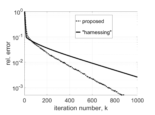
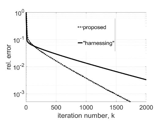
Figure 1: Relative error versus iteration number for the method in [24] (“harnessing”, solid line) and the proposed method (dotted line).

Figure 1 (top) plots the relative error versus number of iterations with the two methods.One can see that the DSG method significantly improves the convergence speed. For example, to reach the relative error $0.01$, the DSG method requires about $340$ iterations, while the method in [24] takes about $560$ iterations for the same target accuracy; this corresponds to savings of about $40\%.$

Figure 1 (bottom) repeats the experiment for a $n=100$-node connected random geometric graph, with the remaining data and network parameters as before. We can see that the DSG method achieves similar gains. For example, for the $0.01$ accuracy, the DSG method needs about $650$ iterations, while the method in [24] needs about $1150$, corresponding to decrease of about $43\%$ in computational costs. We also report that the method in [24] and step-size equal to $1/{\sigma}_{\min}=10/(3L)$ diverges.

6 Conclusion

The method proposed in this paper, DSG, is a distributed version of the Spectral Gradient method for unconstrained optimization problems. Following the approach of exact distributed gradient methods in [21] and [24], at each iteration the nodes update two quantities – the local approximation of the solution and the local approximation of the average gradient. The key novelty developed here is the step size selection which is defined in a spectral-like manner. Each node approximates the local Hessian by a scalar matrix thereby incorporating a degree of second order information in the gradient method. The spectral-like step-size coefficients are derived by exploiting an analogy with the error dynamics of the classical spectral method for quadratic functions and embedding this dynamics into a primal-dual framework. This step-size calculation is computationally cheap and does not incur additional communication overhead. Under a set of standard assumptions regarding the objective functions and assuming a connected communication network, the DSG method generates a sequence of iterates which converges R-linearly to the exact solution of the aggregate objective function. The spectral gradient method is well known for its efficiency in classical, centralized optimization. Preliminary numerical tests demonstrate similar gains of incorporating spectral step-sizes in the distributed setting as well.

References

• [1] Barzilai J, Borwein JM, Two Point Step Size Gradient Methods, IMA Journal of Numerical Analysis, 8 (1988), 141 - 148.
• [2] Birgin, E.G, Martínez, J.M, Raydan M., Nonmonotone Spectral Projected Gradient Methods on Convex Sets, SIAM Journal on Optimization, 10, (2000), 1196-1211.
• [3] Birgin, E.G., Martínez, J.M., Raydan M., Algorithm 813: SPG - Software for Convex- Constrained Optimization, ACM Transactions on Mathematical Software, 27 (2001), 340-349.
• [4] Birgin, E.G., Martínez, J.M., Raydan M Inexact Spectral Projected Gradient Methods on Convex Sets, IMA Journal of Numerical Analysis, 23, (2003), 539-559.
• [5] Birgin, E.G., Martínez, J.M., Raydan M Spectral Projected Gradient Methods: Review and Perspectives, Journal of Statistical Software 60(3), (2014), 1-21.
• [6] Boyd, S., Parikh, N., Chu, E., Peleato, B., Eckstein, J., Distributed optimization and statistical learning via the alternating direction method of multipliers, Foundations and Trends in Machine Learning, Volume 3, Issue 1, (2011) pp. 1-122.
• [7] Cattivelli, F., Sayed, A. H., Diffusion LMS strategies for distributed estimation, IEEE Transactions on Signal Processing, vol. 58, no. 3, (2010) pp. 1035–1048.
• [8] Dai, Y.H., Liao, L.Z., R-Linear Convergence of the Barzilai and Borwein Gradient Method, IMA Journal on Numerical Analysis, 22 (2002), 1-10.
• [9] Desoer, C., Vidyasagar, M., Feedback Systems: Input-Output Properties, SIAM 2009.
• [10] Jakovetić, D., A Unification and Generalization of Exact Distributed First Order Methods, arxiv preprint, arXiv:1709.01317, 2017.
• [11] Jakovetić, D., Xavier, J., Moura, J. M. F., Fast distributed gradient methods, IEEE Transactions on Automatic Control, vol. 59, no. 5, (2014) pp. 1131–1146.
• [12] Jakovetić, D., Moura, J. M. F., Xavier, J., Distributed Nesterov-like gradient algorithms, in CDC’12, 51${}^{\textrm{st}}$ IEEE Conference on Decision and Control, Maui, Hawaii, December 2012, pp. 5459–5464.
• [13] Jakovetić, D., Bajović, D., Krejić, N., Krklec Jerinkić, N., Newton-like Method with Diagonal Correction for Distributed Optimization, SIAM J. Optimization, 27 (2), (2017), 1171-1203.
• [14] Kar, S., Moura, J. M. F., Ramanan, K., Distributed parameter estimation in sensor networks: Nonlinear observation models and imperfect communication, IEEE Transactions on Information Theory, vol. 58, no. 6, (2012) pp. 3575–3605.
• [15] Kar, S., Moura, J. M. F., Distributed Consensus Algorithms in Sensor Networks With Imperfect Communication: Link Failures and Channel Noise, IEEE Transactions on Signal Processing, vol. 57, no. 1, (2009) pp. 355–369.
• [16] Lopes, C., Sayed, A. H., Adaptive estimation algorithms over distributed networks, in 21st IEICE Signal Processing Symposium, Kyoto, Japan, Nov. 2006.
• [17] Mokhtari, A., Ling, Q., Ribeiro, A., Network Newton–Part I: Algorithm and Convergence, 2015, available at: http://arxiv.org/abs/1504.06017
• [18] A. Mokhtari, W. Shi, Q. Ling, and A. Ribeiro, DQM: Decentralized Quadratically Approximated Alternating Direction Method of Multipliers, to appear in IEEE Trans. Sig. Process., 2016, DOI: 10.1109/TSP.2016.2548989
• [19] A. Mokhtari, W. Shi, Q. Ling, and A. Ribeiro, A Decentralized Second Order Method with Exact Linear Convergence Rate for Consensus Optimization, 2016, available at: http://arxiv.org/abs/1602.00596
• [20] Mota, J., Xavier, J., Aguiar, P., Püschel, M., Distributed optimization with local domains: Applications in MPC and network flows, to appear in IEEE Transactions on Automatic Control, 2015.
• [21] Nedic, A., Olshevsky, A., Shi, W., Uribe, C.A., Geometrically convergent distributed optimization with uncoordinated step-sizes, arXiv preprint, arXiv:1609.05877, 2016.
• [22] Nedic, A., Olshevsky, A., Shi, W., Achieving Geometric Convergence for Distributed Optimization over Time-Varying Graphs, arxiv preprint, arXiv:1607.03218, 2016.
• [23] Nedić, A., Ozdaglar, A., Distributed subgradient methods for multi-agent optimization, IEEE Transactions on Automatic Control, vol. 54, no. 1, (2009) pp. 48–61.
• [24] Qu, G., Li, N., Harnessing smoothness to accelerate distributed optimization, IEEE Transactions on Control of Network Systems (to appear)
• [25] Raydan, M., On the Barzilai and Borwein Choice of Steplength for the Gradient Method, IMA Journal of Numerical Analysis, 13 (1993), 321- 326.
• [26] Raydan M, Barzilai and Borwein Gradient Method for the Large Scale Unconstrained Minimization Problem, SIAM Journal on Optimization 7 (1997), 26 - 33.
• [27] Schizas, I. D. , Ribeiro, A., Giannakis, G. B., Consensus in ad hoc WSNs with noisy links – Part I: Distributed estimation of deterministic signals, IEEE Transactions on Signal Processing, vol. 56, no. 1, (2009) pp. 350–364.
• [28] Shi, W., Ling, Q., Wu, G., Yin, W., EXTRA: an Exact First-Order Algorithm for Decentralized Consensus Optimization, SIAM Journal on Optimization, No. 25 vol. 2, (2015) pp. 944-966.