Model-Free Tests for Series Correlation in Multivariate Linear Regression

Abstract.

Testing for series correlation among error terms is a basic problem in linear regression model diagnostics. The famous Durbin-Watson test and Durbin’s h-test rely on certain model assumptions about the response and regressor variables. The present paper proposes simple tests for series correlation that are applicable in both fixed and random design linear regression models. The test statistics are based on the regression residuals and design matrix. The test procedures are robust under different distributions of random errors. The asymptotic distributions of the proposed statistics are derived via a newly established joint central limit theorem for several general quadratic forms and the delta method. Good performance of the proposed tests is demonstrated by simulation results.

1. Introduction

Linear regression is an important topic in statistics and has been found to be useful in almost all aspects of data science, especially in business and economics statistics and biostatistics. Consider the following multivariate linear regression model

(1.1) $$\mathbb{Y}=\mathbb{X}^{\prime}\mathbf{\beta}+{{\varepsilon}},$$

where $\mathbb{Y}$ is the response variable, $\mathbb{X}=(x_{1},x_{2},\cdots,x_{p})^{\prime}$ is a $p$-dimensional vector of regressors, $\beta=\left(\beta_{1},\beta_{2},\cdots,\beta_{p}\right)^{\prime}$ is a $p$-dimensional regression coefficient vector and $\boldsymbol{\varepsilon}$ is random errors with zero mean. Suppose we obtain $n$ samples from this model, that is, $\mathbf{Y}=(y_{1},y_{2},\cdots,y_{n})^{\prime}$ with design matrix $\mathbf{X}=(\mathbf{x}_{1},\mathbf{x}_{2},\cdots,\mathbf{x}_{n})^{\prime}$, where for $i=1,\cdots,n$, $\mathbf{x}_{i}=\left(\mathbf{x}_{i1},\mathbf{x}_{i2},\cdots,\mathbf{x}_{ip}\right)^{\prime}$. The first task in a regression problem is to make statistical inference about the regression coefficient vector. By applying the ordinary least squares (OLS) method, we obtain the estimate $\hat{\beta}=\left(\mathbf{X}^{\prime}\mathbf{X}\right)^{-1}\mathbf{X}^{\prime}\mathbf{Y}$ for coefficient vector $\beta$. In most applications of linear regression models, we need the assumption that the random errors $\{\varepsilon_{i}\}_{i=1}^{n}$ are uncorrelated and homoscedastic. That is to say, we assume

$${\rm Cov}\left(\varepsilon_{i},\varepsilon_{j}\right)=\begin{cases}\sigma^{2}&\mbox{for $i=j$,}\\ 0&\mbox{for $i\neq j$},\end{cases}$$

where $\sigma^{2}$ are unknown. With this assumption, the Gauss-Markov theorem states that the ordinary least squares estimate (OLSE) $\hat{\beta}$ is the best linear unbiased estimator (BLUE). When this assumption does not hold, we suffer from a loss of efficiency and, even worse, make wrong inferences in using OLS. For example, positive serial correlation in the regression error terms will typically lead to artificially small standard errors for the regression coefficient when we apply the classic linear regression method, which will cause the estimated t-statistic to be inflated, indicating significance even when there is in fact none. Therefore, tests for heteroscedasticity and series correlation are important when applying linear regression.

For detecting heteroscedasticity, in one of the most cited papers in econometrics, White [White(1980)] proposed a test based on comparing the Huber-White covariance estimator to the usual covariance estimator under homoscedasticity. Many other researchers have considered this problem, for example, Breusch and Pagan [Breusch and Pagan(1979)], Dette and Munk [Dette and Munk(1998)], Glejser [Glejser(1969)], Harrison and McCabe [Harrison and McCabe(1979)], Cook and Weisberg [Cook and Weisberg(1983)], and Azzalini and Bowman[Azzalini and Bowman(1993)]. Recently, Li and Yao [Li and Yao(2015)] and Bai, Pan and Yin [Bai et al.(2018)Bai, Pan, and Yin] proposed tests for heteroscedasticity that are valid in both low- and high-dimensional regressions. Their tests were shown by simulations to perform better than some classic tests.

The most famous test for series correlation, the Durbin-Watson test, was proposed in [Durbin and Watson(1950), Durbin and Watson(1951), Durbin and Watson(1971)]. The Durbin-Watson test statistic is based on the residuals $e_{1},e_{2},\cdots,e_{n}$ from linear regression. The researchers considered the statistic

$$d=\frac{\sum_{i=2}^{n}\left(e_{i}-e_{i-1}\right)^{2}}{\sum_{i=1}^{n}e_{i}^{2}},$$

whose small-sample distribution was derived by John von Neumann. In the original papers, Durbin and Watson investigated the distribution of this statistic under the classic independent framework, described the test procedures and provided tables of the bounds of significance. However, the asymptotic results were derived under the normality assumption on the error term, and as noted by Nerlove and Wallis [Nerlove and Wallis(1966)], although the Durbin-Watson test appeared to work well in an independent observations framework, it may be asymptotically biased and lead to inadequate conclusions for linear regression models containing lagged dependent random variables. New alternative test procedures, for instance, Durbin’s h-test and t-test [Durbin(1970)], were proposed to address this problem; see also Inder [Inder(1986)], King and Wu [King and Wu(1991)], Stocker [Stocker(2007)], Bercu and Proïa [Bercu and Proia(2013)], Gençay and Signori [Gençay and Signori(2015)] and Li and Gençay [Li and Gençay(2017)] and references therein. However, all these tests were proposed under some model assumptions on the regressors and/or the response variable. Moreover, Durbin’s h-test requires a Gaussian distribution of the error term. Thus, some common models are excluded. In fact, since it is difficult to assess whether the regressors and/or the response are lag dependent, model-free tests for the regressors and response variable appear to be appropriate.

The present paper proposes a simple test procedure without assumptions on the response variable and regressors that is valid in both low- and high-dimensional multivariate linear regression. The main idea, which is simple but proves to be useful, is to express the mean and variance of the test statistic by making use of the residual maker matrix. In addition to a general joint central limit theorem for several quadratic forms, which is proved in this paper and may have its own interest, we consider a Box-Pierce-type test for series correlation. Monte Carlo simulations show that our test procedures perform well in situations where some classic test procedures are inapplicable.

2. Test for series correlation in linear regression model

2.1. Notation

Let $\mathbf{X}$ be the design matrix, and let $\mathbf{R}=(r_{i,j})=\mathbf{I}_{n}-\mathbf{X}(\mathbf{X}^{\prime}\mathbf{X})^{-1}\mathbf{X}^{\prime}$ be the residual maker matrix, where $\mathbf{H}=(h_{i,j})=\mathbf{X}(\mathbf{X}^{\prime}\mathbf{X})^{-1}\mathbf{X}^{\prime}$ is the hat matrix (also known as the projection matrix). We assume that the noise vector $\boldsymbol{\varepsilon}=\mathbf{\Sigma}^{1/2}\boldsymbol{\epsilon},$ where $\boldsymbol{\epsilon}$ is an $n$-dimensional random vector whose entries $\epsilon_{1},\cdots,\epsilon_{n}$ are independent with zero means, unit variances and the same finite fourth-order moments $M_{4}$, and $\mathbf{\Sigma}^{1/2}$ is an n-dimensional nonnegative definite nonrandom matrix with bounded spectral norm. Then, the OLS residuals are ${\mathbf{e}}=(e_{1},\cdots,e_{n})^{\prime}=\mathbf{R}\mathbf{\Sigma}^{1/2}\boldsymbol{\epsilon}$. We note that we will use $\circ$ to indicate the Hadamard product of two matrices in the rest of this paper.

2.2. Test for a given order series correlation

To test for a given order series correlation, for any number $q\leq n$, denote

$$\gamma_{\tau}=\sum_{i={\tau+1}}^{n}e_{i}e_{i-\tau}=\mathbf{e}^{\prime}\mathbf{P}_{\tau}\mathbf{e}=\boldsymbol{\epsilon}^{\prime}\mathbf{\Sigma}^{1/2}\mathbf{R}\mathbf{P}_{\tau}\mathbf{R}\mathbf{\Sigma}^{1/2}\boldsymbol{\epsilon},\quad\tau=0,\cdots,q,$$

where $\mathbf{P}_{\tau}=\left(p_{i,j}^{(\tau)}\right)_{n\times n}$ with $p_{i,j}^{(\tau)}=\begin{cases}1&\mbox{for $i-j=\tau$,}\\ 0&\mbox{other}.\end{cases}$

First, for $0\leq\tau\leq q,$ we have

(2.1) $${\rm E}\gamma_{\tau}={\rm E}{\rm tr}\boldsymbol{\epsilon}^{\prime}\mathbf{\Sigma}^{1/2}\mathbf{R}\mathbf{P}_{\tau}\mathbf{R}\mathbf{\Sigma}^{1/2}\boldsymbol{\epsilon}={\rm tr}\mathbf{\Sigma}^{1/2}\mathbf{R}\mathbf{P}_{\tau}\mathbf{R}\mathbf{\Sigma}^{1/2}={\rm tr}\mathbf{R}\mathbf{P}_{\tau}\mathbf{R}\mathbf{\Sigma}.$$

Denote $\mathbf{\Sigma}^{1/2}\mathbf{R}\mathbf{P}_{\tau_{1}}\mathbf{R}\mathbf{\Sigma}^{1/2}=(a_{i,j})$ and $\mathbf{\Sigma}^{1/2}\mathbf{R}\mathbf{P}_{\tau_{2}}\mathbf{R}\mathbf{\Sigma}^{1/2}=(b_{i,j})$, and set $\nu_{4}=M_{4}-3;$ we then have, for $\tau_{1},\tau_{2}=0,\cdots,q,$

(2.2) $${\rm Cov}(\gamma_{\tau_{1}},\gamma_{\tau_{2}})$$

$$= {\rm E}\left(\boldsymbol{\epsilon}^{\prime}\mathbf{\Sigma}^{1/2}\mathbf{R}\mathbf{P}_{\tau_{1}}\mathbf{R}\mathbf{\Sigma}^{1/2}\boldsymbol{\epsilon}-{\rm tr}\mathbf{R}\mathbf{P}_{\tau_{1}}\mathbf{R}\mathbf{\Sigma}\right)\left(\boldsymbol{\epsilon}^{\prime}\mathbf{\Sigma}^{1/2}\mathbf{R}\mathbf{P}_{\tau_{2}}\mathbf{R}\mathbf{\Sigma}^{1/2}\boldsymbol{\epsilon}-{\rm tr}\mathbf{R}\mathbf{P}_{\tau_{2}}\mathbf{R}\mathbf{\Sigma}\right)$$

$$= {\rm E}\left(\sum_{i}a_{i,i}\left(\epsilon_{i}^{2}-1\right)+\sum_{i\neq j}a_{i,j}\epsilon_{i}\epsilon_{j}\right)\left(\sum_{i}b_{i,i}\left(\epsilon_{i}^{2}-1\right)+\sum_{i\neq j}b_{i,j}\epsilon_{i}\epsilon_{j}\right)$$

$$= \nu_{4}{\rm tr}\left(\left(\mathbf{\Sigma}^{1/2}\mathbf{R}\mathbf{P}_{\tau_{1}}\mathbf{R}\mathbf{\Sigma}^{1/2}\right)\circ\left(\mathbf{\Sigma}^{1/2}\mathbf{R}\mathbf{P}_{\tau_{2}}\mathbf{R}\mathbf{\Sigma}^{1/2}\right)\right)+{\rm tr}\left(\mathbf{\Sigma}^{1/2}\mathbf{R}\mathbf{P}_{\tau_{1}}\mathbf{R}\mathbf{\Sigma}^{1/2}\right)\left(\mathbf{\Sigma}^{1/2}\mathbf{R}\mathbf{P}_{\tau_{2}}\mathbf{R}\mathbf{\Sigma}^{1/2}\right)$$

$$+{\rm tr}\left(\mathbf{\Sigma}^{1/2}\mathbf{R}\mathbf{P}_{\tau_{1}}\mathbf{R}\mathbf{\Sigma}^{1/2}\right)\left(\mathbf{\Sigma}^{1/2}\mathbf{R}\mathbf{P}_{\tau_{2}}\mathbf{R}\mathbf{\Sigma}^{1/2}\right)^{\prime}$$

$$= \nu_{4}{\rm tr}\left(\left(\mathbf{\Sigma}^{1/2}\mathbf{R}\mathbf{P}_{\tau_{1}}\mathbf{R}\mathbf{\Sigma}^{1/2}\right)\circ\left(\mathbf{\Sigma}^{1/2}\mathbf{R}\mathbf{P}_{\tau_{2}}\mathbf{R}\mathbf{\Sigma}^{1/2}\right)\right)+{\rm tr}\mathbf{P}_{\tau_{1}}\mathbf{R}\mathbf{\Sigma}\mathbf{R}\mathbf{P}_{\tau_{2}}\mathbf{R}\mathbf{\Sigma}\mathbf{R}+{\rm tr}\mathbf{P}_{\tau_{1}}\mathbf{R}\mathbf{\Sigma}\mathbf{R}\mathbf{P}^{\prime}_{\tau_{2}}\mathbf{R}\mathbf{\Sigma}\mathbf{R}.$$

Note that ${\rm Cov}\left(\boldsymbol{\varepsilon},\boldsymbol{\varepsilon}\right)=\mathbf{\Sigma}.$ We want to test the hypothesis for $1\leq\tau\leq q,$

$$H_{0}:\mathbf{\Sigma}=\sigma^{2}\mathbf{I}_{n},\quad{\mbox{where}\ }0<\sigma^{2}<\infty,$$

against

$$H_{1,\tau}:{\rm Cov}(\varepsilon_{i},\varepsilon_{i-\tau})=\rho\neq 0.$$

Under the null hypothesis, due to (2.1) and (2.2), we obtain

(2.3) $${\rm E}\gamma_{\tau}=\sigma^{2}{\rm tr}\mathbf{P}_{\tau}\mathbf{R},$$

and

(2.4) $${\rm Cov}(\gamma_{\tau_{1}},\gamma_{\tau_{2}})=\sigma^{4}\left(\nu_{4}{\rm tr}\left(\left(\mathbf{R}\mathbf{P}_{\tau_{1}}\mathbf{R}\right)\circ\left(\mathbf{R}\mathbf{P}_{\tau_{2}}\mathbf{R}\right)\right)+{\rm tr}\mathbf{P}_{\tau_{1}}\mathbf{R}\mathbf{P}_{\tau_{2}}\mathbf{R}+{\rm tr}\mathbf{P}_{\tau_{1}}\mathbf{R}\mathbf{P}^{\prime}_{\tau_{2}}\mathbf{R}\right).$$

Specifically, we have ${\rm E}\gamma_{\tau_{0}}=\sigma^{2}{\rm tr}\mathbf{R}=\sigma^{2}(n-p)$ and

(2.5) $${\rm Var}(\gamma_{\tau_{0}})=\sigma^{4}\left(\nu_{4}{\rm tr}\left(\mathbf{R}\circ\mathbf{R}\right)+2(n-p)\right).$$

The validity of our test procedure requires the following mild assumptions.

(1): Assumption on $p$ and $n$:

The number of regressors $p$ and the sample size $n$ satisfy that $p/n\to c\in[0,1)$ as $n\to\infty$.

(2): Assumption on errors:

The fourth-order cumulant of the error distribution $\nu_{4}\neq-2$.

Assumption $(2)$ excludes the rare case where the random errors are drawn from a two-point distribution with the same masses $1/2$ at $--1$ and $1$. However, if this situation occurs, our test remains valid if the design matrix satisfies the mild condition that

$$\limsup_{n\to\infty}\frac{{\rm tr}\mathbf{R}\circ\mathbf{R}}{n-p}=\limsup_{n\to\infty}\frac{\sum_{i=1}^{n}r_{i,i}^{2}}{\sum_{i=1}^{n}r_{i,i}}<1.$$

These assumptions ensure that ${\rm Var}(\gamma_{\tau_{0}})$ has the same order as $n$ as $n\to\infty$, thus satisfying the condition assumed in Theorem 4.1.

Define

$$m_{\tau}=\frac{{\rm E}\gamma_{\tau}}{\sigma^{2}}={\rm tr}\mathbf{P}_{\tau}\mathbf{R},\quad v_{\tau_{1}\tau_{2}}=\frac{{\rm Cov}(\gamma_{\tau_{1}},\gamma_{\tau_{2}})}{n\sigma^{4}}.$$

By applying Theorem 4.1 presented in Section 4, we obtain that for $1\leq\tau\leq q,$

$$\frac{1}{\sqrt{n}}\left(\left(\begin{array}[]{c}\gamma_{\tau}\\ \gamma_{0}\\ \end{array}\right)-\left(\begin{array}[]{c}m_{\tau}\\ m_{0}\\ \end{array}\right)\right)\sim N\left(\mathbf{0},\left(\begin{array}[]{cc}v_{{\tau}{\tau}}&v_{{\tau}0}\\ v_{0{\tau}}&v_{00}\\ \end{array}\right)\right).$$

Then, by the delta method, we obtain, as $n\to\infty$,

$$T_{\tau}=\frac{\sqrt{n}\left(\frac{\gamma_{\tau}}{\gamma_{0}}-\mu_{{\tau}0}\right)}{\sigma_{{\tau}0}}\sim N(0,1),$$

where $\mu_{{\tau}0}=\frac{m_{\tau}}{m_{0}}$ and

(2.11) $$\sigma_{{\tau}0}^{2}= \left(\begin{array}[]{cc}\frac{1}{m_{0}/n}&\frac{m_{1}/n}{\left(m_{0}/n\right)^{2}}\\ \end{array}\right)\left(\begin{array}[]{cc}v_{{1}{1}}&v_{{1}0}\\ v_{0{1}}&v_{00}\\ \end{array}\right)\left(\begin{array}[]{c}\frac{1}{m_{0}/n}\\ \frac{m_{1}/n}{\left(m_{0}/n\right)^{2}}\\ \end{array}\right)$$

(2.17) $$= n^{2}\left(\begin{array}[]{cc}\frac{1}{n-p}&\frac{m_{1}}{(n-p)^{2}}\\ \end{array}\right)\left(\begin{array}[]{cc}v_{{1}{1}}&v_{{1}0}\\ v_{0{1}}&v_{00}\\ \end{array}\right)\left(\begin{array}[]{c}\frac{1}{n-p}\\ \frac{m_{1}}{(n-p)^{2}}\\ \end{array}\right).$$

We reject $H_{0}$ in favor of $H_{1,\tau}$ if a large $|T_{\tau}|$ is observed.

2.3. A portmanteau test for series correlation

In time series analysis, the Box-Pierce test proposed in [Box and Pierce(1970)] and the Ljung-Box statistic proposed in [Ljung and Box(1978)] are two portmanteau tests of whether any of a group of autocorrelations of a time series are different from zero. For a linear regression model, consider the following hypothesis

$$H_{0}:\mathbf{\Sigma}=\sigma^{2}\mathbf{I}_{n},$$

against

$$H_{1}:{\mbox{there\ exist}}\ 1\leq\tau\leq q\ {\mbox{such\ that}}\ {\rm Cov}(\varepsilon_{i},\varepsilon_{i-\tau})=\rho\neq 0.$$

Applying Theorem 4.1 and the delta method, we shall now consider the following asymptotically standard normally distributed statistic

$$T(q)=\frac{\sqrt{n}\left(\sum_{\tau=1}^{q}\left({2-\frac{\gamma_{\tau}}{\gamma_{0}}}\right)^{2}-\sum_{\tau=1}^{q}(2-{\mu_{\tau 0}})^{2}\right)}{\sigma_{T}}\sim N(0,1),$$

as $n\to\infty,$ where $\mu_{\tau 0}=\frac{m_{\tau}}{m_{0}}$ and $\sigma_{T}=\sqrt{{\nabla}^{\prime}{\Sigma}_{T}\nabla}$ with

$${\nabla}=\left(\frac{2n\sum_{\tau=1}^{q}m_{\tau}(2-\frac{m_{\tau}}{n-p})}{(n-p)^{2}},\frac{-2n(2-\frac{m_{1}}{n-p})}{(n-p)},\frac{-2n(2-\frac{m_{2}}{n-p})}{(n-p)},\cdots,\frac{-2n(2-\frac{m_{q}}{n-p})}{(n-p)}\right)^{\prime},$$

and

$${\Sigma}_{T}=\left(v_{i,j}\right)_{(q+1)\times(q+1)},\quad i,j=0,\cdots,q.$$

Then, we reject $H_{0}$ in favor of $H_{1}$ if $|T(q)|$ is large.

2.4. Discussion of the statistics

In the present subsection, we discuss the asymptotic parameters of the two proposed statistics.

If the entries in design matrix $\mathbf{X}$ are assumed to be i.i.d. standard normal, then we know that as $n\to\infty$, the diagonal entries in the symmetric and idempotent matrices $\mathbf{H}$ and $\mathbf{R}=\mathbf{I}_{n}-\mathbf{H}$ are of constant order while the off-diagonal entries are of order $n^{-1/2}$. Then, the order of $m_{\tau}={\rm tr}\mathbf{P}_{\tau}\mathbf{R}$ for a given $\tau>0$ is at most $n^{1/2}$ since it is exactly the summation of the $n-\tau$ off-diagonal entries of $\mathbf{R}$. Thus, elementary analysis shows that $\sigma_{{\tau}0}^{2}=\frac{n^{2}v_{11}}{(n-p)^{2}}+o(1)$.

For a fixed design or a more general random design, it become almost impossible to study matrices $\mathbf{H}$ and $\mathbf{R}=\mathbf{I}_{n}-\mathbf{H}$, except for some of the elementary properties. Thus, for the purpose of obtaining an accurate statistical inference, we suggest the use of the original parameters since we have little information on the distribution of the regressors in a fixed design, and the calculation of those parameters is not excessively complex.

3. Simulation studies

In this section, Monte Carlo simulations are conducted to investigate the performance of our proposed tests.

3.1. Performance of test for first-order series correlation

First, we consider the test for first-order series correlation of the error terms in multivariate linear regression model (1.1). Note that although our theory results were derived by treating the design matrix as a constant matrix, we also need to obtain a design matrix under a certain random model in the simulations. We thus consider the situation where the regressors $\mathbf{x}_{1},\mathbf{x}_{2},\cdots,\mathbf{x}_{f}$ are lagged dependent. Formally, for a given $f$, we set

$$x_{t,j}=rx_{t-1,j}+u_{t},\quad j=1,\cdots,f,\quad t=1,\cdots,n,$$

where $r=0.2$ and $\{u_{t}\}$ are independently drawn from N(0,1). While $\{x_{i,j}\},f+1\leq j\leq p,1\leq i\leq n$ are independently chosen from a Student’s t-distribution with 5 degrees of freedom. The random errors $\varepsilon$ obey (1) the normal distribution N(0,1) and (2) the uniform distribution U(-1,1). The significant level is set to $\alpha=0.05.$ Table 1 and Table 2 show the empirical size of our test (denoted as $``{\rm FDWT}"$) for different $p,n,f$ under the two error distributions. To investigate the power of our test, we randomly choose a $\varepsilon_{0}$ and consider the following AR(1) model:

$$\varepsilon_{t}=\rho\varepsilon_{t-1}+\vartheta_{t},\quad t=1,\cdots,n$$

where $\{\vartheta_{t}\}$ are independently drawn from (1) N(0,1) and (2) U(-1,1). Tables 3 and 4 show the empirical power of our proposed test for different $p,n,f,\rho$ under the two error distributions.

These simulation results show that our test always has good size and power when $n-p$ is large and is thus applicable under the framework that $p/n\to[0,1)$ as $n\to\infty$.

$p,n$	f	FDWT	$p,n$	f	FDWT
2,32	1	0.0486	8,32	2	0.0428
8,32	4	0.0410	8,32	8	0.0434
16,64	4	0.0446	16,64	12	0.0463
32,64	12	0.0420	32,64	24	0.0414
32,128	12	0.0470	32,128	24	0.0478
64,128	12	0.0479	64,128	36	0.0430
128,256	12	0.0509	128,256	24	0.0486
128,256	64	0.0504	128,256	128	0.0422
128,512	24	0.0519	128,512	64	0.0496
128,512	96	0.0487	128,512	128	0.0497
256,512	64	0.0469	256,512	96	0.0492
256,512	144	0.0472	256,512	256	0.0486
256,1028	64	0.0457	256,1028	96	0.0498
256,1028	144	0.0473	256,1028	256	0.0487
512,1028	12	0.0463	512,1028	96	0.0506
512,1028	144	0.0520	512,1028	256	0.0478
512,1028	288	0.0460	512,1028	314	0.0442
512,1028	440	0.0438	512,1028	512	0.0443

Table 1. Empirical size under Gaussian error assumption

$p,n$	f	FDWT	$p,n$	f	FDWT
2,32	1	0.0410	2,32	2	0.0421
8,32	4	0.0414	8,32	8	0.0468
16,64	4	0.0467	16,64	12	0.0450
32,64	12	0.0450	32,64	24	0.0419
32,128	12	0.0456	32,128	24	0.0458
64,128	12	0.0479	64,128	36	0.0460
128,256	12	0.0509	128,256	24	0.0476
128,256	64	0.0461	128,256	128	0.0412
128,512	24	0.0497	128,512	64	0.0505
128,512	96	0.0508	128,512	128	0.0501
256,512	64	0.0525	256,512	96	0.0455
256,512	144	0.0443	256,512	256	0.0461
256,1028	64	0.0509	256,1028	96	0.0455
256,1028	144	0.0482	256,1028	256	0.0465
512,1028	12	0.0491	512,1028	96	0.0461
512,1028	144	0.0483	512,1028	256	0.0480
512,1028	288	0.0447	512,1028	314	0.0468
512,1028	440	0.0453	512,1028	512	0.0459

Table 2. Empirical size under uniform distribution U(-1,1) error assumption

$p,n$	f	$\rho=0.2$	$\rho=-0.3$	$\rho=0.5$	$p,n$	f	$\rho=0.2$	$\rho=-0.3$	$\rho=0.5$
2,32	1	0.1363	0.2550	0.5409	8,32	2	0.1056	0.1705	0.3224
8,32	4	0.0906	0.1724	0.3841	8,32	8	0.1093	0.1831	0.3597
16,64	4	0.1888	0.3672	0.6783	16,64	12	0.1987	0.3764	0.7199
32,64	12	0.1055	0.1584	0.3542	32,64	24	0.1030	0.1739	0.3791
32,128	12	0.3673	0.6637	0.9552	32,128	24	0.3706	0.6655	0.9556
64,128	12	0.1754	0.3335	0.6345	64,128	36	0.1897	0.3519	0.6639
128,256	12	0.3255	0.6104	0.9160	128,256	24	0.3324	0.6037	0.9225
128,256	64	0.3362	0.6200	0.9345	128,256	128	0.3362	0.6515	0.9438
128,512	24	0.9064	0.9981	1.0000	128,512	64	0.9151	0.9976	1.0000
128,512	96	0.9167	0.9981	1.0000	128,512	128	0.9196	0.9981	1.0000
256,512	64	0.5880	0.8951	0.9975	256,512	96	0.6041	0.9029	0.9980
256,512	144	0.6019	0.8963	0.9990	256,512	256	0.6117	0.9103	0.9987
256,1028	64	0.9970	1.0000	1.0000	256,1028	96	0.9973	1.0000	1.0000
256,1028	144	0.9971	1.0000	1.0000	256,1028	256	0.9976	1.0000	1.0000
512,1028	12	0.8766	0.9957	1.0000	512,1028	96	0.8829	0.9958	1.0000
512,1028	144	0.9201	0.9979	1.0000	512,1028	256	0.8967	0.9954	1.0000
512,1028	288	0.9125	0.9986	1.0000	512,1028	314	0.8946	0.9969	1.0000
512,1028	440	0.8942	0.9975	1.0000	512,1028	512	0.8937	0.9979	1.0000

Table 3. Empirical power under Gaussian error assumption

$p,n$	f	$\rho=0.2$	$\rho=-0.3$	$\rho=0.5$	$p,n$	f	$\rho=0.2$	$\rho=-0.3$	$\rho=0.5$
2,32	1	0.1457	0.2521	0.5548	8,32	2	0.1245	0.1721	0.3478
8,32	4	0.1245	0.1754	0.3548	8,32	8	0.1254	0.1845	0.3547
16,64	4	0.1987	0.3789	0.6567	16,64	12	0.1879	0.3478	0.7456
32,64	12	0.1145	0.1544	0.3582	32,64	24	0.1125	0.1555	0.3548
32,128	12	0.3825	0.6647	0.9845	32,128	24	0.3845	0.6789	0.9677
64,128	12	0.1863	0.3765	0.6748	64,128	36	0.1758	0.3877	0.6478
128,256	12	0.3358	0.5978	0.9185	128,256	24	0.3495	0.6657	0.9244
128,256	64	0.3378	0.5899	0.9578	128,256	128	0.3392	0.6788	0.9584
128,512	24	0.9114	0.9945	1.0000	128,512	64	0.9121	0.9944	1.0000
128,512	96	0.9102	0.9977	1.0000	128,512	128	0.9157	0.9945	0.9999
256,512	64	0.6053	0.8979	0.9969	256,512	96	0.6020	0.9456	0.9978
256,512	144	0.6151	0.8966	1.0000	256,512	256	0.6135	0.9678	1.0000
256,1028	64	0.9975	1.0000	1.0000	256,1028	96	0.9972	1.0000	1.0000
256,1028	144	0.9921	1.0000	1.0000	256,1028	256	0.9982	1.0000	1.0000
512,1028	12	0.8787	0.9944	1.0000	512,1028	96	0.8800	0.9976	1.0000
512,1028	144	0.9201	0.9913	1.0000	512,1028	256	0.8881	0.9964	1.0000
512,1028	288	0.9165	0.9959	1.0000	512,1028	314	0.8957	0.9967	1.0000
512,1028	440	0.8978	0.9944	1.0000	512,1028	512	0.8959	0.9947	1.0000

Table 4. Empirical power under uniform distribution U(-1,1) error assumption

3.2. Performance of the Box-Pierce type test

This subsection investigates the performance of our proposed Box-Pierce type test statistic $T(q)$ in subsection 2.3. The design matrix $\mathbf{X}$ is obtained in the same way as in the last subsection, with $f=p/2$, and the random error terms are assumed to obey a (1) normal distribution N(0,1) and a (2) gamma distribution with parameters 4 and 1/2. Table 5 and Table 6 show the empirical size of our test with different $n,p,q$ under the two error distributions. We consider the following AR(2) model to assess the power:

$$\varepsilon_{t}=\rho_{1}\varepsilon_{t-1}+\rho_{2}\varepsilon_{t-2}+\vartheta_{t},\quad t=1,\cdots,n$$

where $\{\vartheta_{t}\}$ are independently drawn from (1) N(0,1) and (2) Gamma(4,1/2). The design matrix $\mathbf{X}$ is obtained in the same way as before, with $f=p/2$. Tables 7 and 8 show the empirical power of our proposed test for different $p,n,\rho$ under the two error distributions.

As shown by these simulation results, the empirical size and empirical power of the portmanteau test improve as $n-p$ tends to infinity.

$p,n$	$n-p$	$q=3$	$q=5$	$p,n$	$n-p$	$q=3$	$q=5$
2,32	30	0.0389	0.0402	8,32	24	0.0351	0.0350
16,32	16	0.0299	0.0349	24,32	8	0.0208	0.0132
2,64	62	0.0443	0.0505	32,64	32	0.0391	0.0420
32,128	96	0.0436	0.0501	64,128	64	0.0402	0.0427
32,256	224	0.0489	0.0470	64,256	192	0.0475	0.0485
128,256	128	0.0452	0.0477	16,512	496	0.0499	0.0494
64,512	448	0.0490	0.0486	128,512	384	0.0502	0.0513
256,512	256	0.0473	0.0438	64,1028	964	0.0461	0.0494
128,1028	900	0.0480	0.0485	256,1028	772	0.0492	0.0501

Table 5. Empirical size under Gaussian error assumption

$p,n$	$n-p$	$q=3$	$q=5$	$p,n$	$n-p$	$q=3$	$q=5$
2,32	30	0.0359	0.0374	8,32	24	0.0390	0.0383
16,32	16	0.0265	0.0281	24,32	8	0.0129	0.0087
2,64	62	0.0444	0.0426	32,64	32	0.0385	0.0365
32,128	96	0.0430	0.0448	64,128	64	0.0439	0.0417
32,256	224	0.0497	0.0437	64,256	192	0.0509	0.0514
128,256	128	0.0487	0.0465	16,512	496	0.0504	0.0498
64,512	448	0.0479	0.0511	128,512	384	0.0498	0.0458
256,512	256	0.0518	0.0523	64,1028	964	0.0500	0.0489
128,1028	900	0.0490	0.0513	256,1028	772	0.0439	0.0503

Table 6. Empirical size under Gamma(4,1/2) error assumption

		$\rho_{1}=0.2$	$\rho_{1}=0$			$\rho_{1}=0.2$	$\rho_{1}=0$
$p,n$	$n-p$	$\rho_{2}=-0.3$	$\rho_{2}=0.3$	$p,n$	$n-p$	$\rho_{2}=-0.3$	$\rho_{2}=0.3$
2,32	30	0.2630	0.1960	8,32	24	0.1699	0.1265
16,32	16	0.0890	0.0694	24,32	8	0.0760	0.0205
2,64	62	0.5698	0.4064	32,64	32	0.1708	0.1210
32,128	96	0.6660	0.4775	64,128	64	0.2764	0.2232
32,256	224	0.9849	0.9278	64,256	192	0.9369	0.8167
128,256	128	0.6147	0.4335	16,512	496	1.0000	1.0000
64,512	448	1.0000	1.0000	128,512	384	0.9991	0.9897
256,512	256	0.9155	0.7551	64,1028	964	1.0000	1.0000
128,1028	900	1.0000	1.0000	256,1028	772	1.0000	1.0000

Table 7. Empirical power under Gaussian error assumption

		$\rho_{1}=0.2$	$\rho_{1}=0$			$\rho_{1}=0.2$	$\rho_{1}=0$
$p,n$	$n-p$	$\rho_{2}=-0.3$	$\rho_{2}=0.3$	$p,n$	$n-p$	$\rho_{2}=-0.3$	$\rho_{2}=0.3$
2,32	30	0.2657	0.1892	8,32	24	0.1202	0.1822
16,32	16	0.0519	0.0281	24,32	8	0.0202	0.0198
2,64	62	0.5721	0.3981	32,64	32	0.1190	0.1998
32,128	96	0.6738	0.5285	64,128	64	0.2853	0.1757
32,256	224	0.9291	0.8898	64,256	192	0.9034	0.7370
128,256	128	0.6320	0.4225	16,512	496	1.0000	0.9998
64,512	448	1.0000	0.9989	128,512	384	0.9989	0.9893
256,512	256	0.9137	0.7530	64,1028	964	1.0000	1.0000
128,1028	900	1.0000	1.0000	256,1028	772	1.0000	1.0000

Table 8. Empirical power under Gamma(4,1/2) error assumption

3.3. Parameter estimation under the null hypothesis

In practice, if the error terms are not Gaussian, we need to estimate the fourth-order cumulant to perform the test. We now give a suggested estimate under the additional assumption that the error terms are independent under the null hypothesis. Note that an unbiased estimate of variance $\sigma^{2}$ under the null hypothesis is

$$\hat{\sigma}_{n}^{2}=\frac{\gamma_{0}}{n-p},$$

and

$$E\sum_{i=1}^{n}e_{i}^{4} =3\sigma^{4}\sum_{i=1}^{n}\sum_{j_{1},j_{2}}h_{ij_{1}}^{2}h_{ij_{2}}^{2}+\nu_{4}\sigma^{4}\sum_{i=1}^{n}\sum_{j=1}^{n}h_{ij}^{4}=3\sigma^{4}{\rm tr}(\mathbf{R}\circ\mathbf{R})+\nu_{4}\sigma^{4}{\rm tr}(\mathbf{R}\circ\mathbf{R})^{2}.$$

Then, $\nu_{4}$ can be estimated by a consistent estimator

$$\hat{\nu}_{4}=\frac{\sum_{i=1}^{n}e_{i}^{4}-3\hat{\sigma}_{n}^{4}{\rm tr}(\mathbf{R}\circ\mathbf{R})}{\hat{\sigma}_{n}^{4}{\rm tr}(\mathbf{R}\circ\mathbf{R})^{2}}.$$

4. A general joint CLT for several general quadratic forms

In this section, we establish a general joint CLT for several general quadratic forms, which helps us to find the asymptotic distribution of the statistics for testing the series correlations. We believe that the result presented below may have its own interest.

4.1. A brief review of random quadratic forms

Quadratic forms play an important role not only in mathematical statistics but also in many other branches of mathematics, such as number theory, differential geometry, linear algebra and differential topology. Suppose ${{\boldsymbol{\varepsilon}}}=\left(\varepsilon_{1},\varepsilon_{2},\cdots,\varepsilon_{n}\right)^{\prime}$, where $\{\varepsilon_{i}\}_{i=1}^{n}$ is a sample of size $n$ drawn from a certain standardized population. Let $\mathbf{A}=(a_{ij})_{n\times n}$ be a matrix. Then, ${{\boldsymbol{\varepsilon}}}^{\prime}\mathbf{A}{{\boldsymbol{\varepsilon}}}=\sum_{i,j}a_{ij}\varepsilon_{i}\varepsilon_{j}$ is called a random quadratic form in $\boldsymbol{\varepsilon}$. The random quadratic forms of normal variables, especially when $\mathbf{A}$ is symmetric, have been considered by many authors, who have achieved fruitful results. We refer the reader to [Bartlett et al.(1960)Bartlett, Gower, and Leslie, Darroch(1961), Gart(1970), Hsu et al.(1999)Hsu, Prentice, Zhao, and Fan, Forchini(2002), Dik and De Gunst(2010), Al-Naffouri et al.(2016)Al-Naffouri, Moinuddin, Ajeeb, Hassibi, and Moustakas]. Furthermore, many authors have considered the more general situation, where $\boldsymbol{\varepsilon}$ follow a non-Gaussian distribution. For the properties of those types of random quadratic forms, we refer the reader to [Fox and Taqqu(1985), Cambanis et al.(1985)Cambanis, Rosinski, and Woyczynski, de Jong(1987), Gregory and Hughes(1995), Gotze and Tikhomirov(1999), Liu et al.(2009)Liu, Tang, and Zhang, Deya and Nourdin(2014), Oliveira(2016)] and the references therein.

However, few studies have considered the joint distribution of several quadratic forms. Thus, in this paper, we want to establish a general joint CLT for several random quadratic forms with general distributions.

4.2. Assumptions and results

To this end, suppose

$$\mathbf{\Xi}=\left(\begin{array}[]{cccc}\varepsilon_{1}^{(1)}&\varepsilon_{2}^{(1)}&\cdots&\varepsilon_{n}^{(1)}\\ \varepsilon_{1}^{(2)}&\varepsilon_{2}^{(2)}&\cdots&\varepsilon_{n}^{(2)}\\ \vdots&\ddots&&\vdots\\ \varepsilon_{1}^{(q)}&\varepsilon_{2}^{(q)}&\cdots&\varepsilon_{n}^{(q)}\\ \end{array}\right)$$

is a $q\times n$ random matrix. Let $\{\mathbf{A}_{l}=a_{i,j}^{(l)}\},1\leq i,j\leq n,1\leq l\leq q$ be $q$ nonrandom $n$-dimensional matrices. Define $Q_{l}=\sum_{i,j=1}^{n}a_{i,j}^{(l)}\varepsilon_{i}^{(l)}\varepsilon_{j}^{(l)}$ for $1\leq l\leq q.$ We are interested in the asymptotic distribution, as $n\to\infty$, of the random vector $\left(Q_{1},Q_{2},\cdots,Q_{q}\right)$, which consists of $q$ random quadratic forms. Now, we make the following assumptions.

• $\{\varepsilon_{j}^{(i)}\}_{1\leq j\leq n,1\leq i\leq q}$ are standard random variables (mean zero and variance one) with uniformly bounded fourth-order moments $M_{4,j}^{(i)}$.

• The columns of $\mathbf{\Xi}$ are independent.

• The spectral norms of the $q$ $n\times n$ square matrices $\{\mathbf{A}_{l}\}_{1\leq l\leq q}$ are uniformly bounded in $n$.

Clearly, for $1\leq l\leq q$, we have ${\rm E}Q_{l}={\rm tr}\mathbf{A}_{l}$, and for $1\leq l_{1},l_{2}\leq q$, we obtain

(4.1) $${{\rm Cov}\left(Q_{l_{1}},Q_{l_{2}}\right)}={\rm E}\left(Q_{l_{1}}-{\rm E}Q_{l_{1}}\right)\left(Q_{l_{2}}-{\rm E}Q_{l_{2}}\right)$$

$$= {\rm E}\left(\sum_{i=1}^{n}a_{i,i}^{(l_{1})}\left(\left(\varepsilon_{i}^{(l_{1})}\right)^{2}-1\right)+\sum_{i\neq j}a_{i,j}^{(l_{1})}\varepsilon_{i}^{(l_{1})}\varepsilon_{j}^{(l_{1})}\right)\left(\sum_{i=1}^{n}a_{i,i}^{(l_{2})}\left(\left(\varepsilon_{i}^{(l_{2})}\right)^{2}-1\right)+\sum_{i\neq j}a_{i,j}^{(l_{2})}\varepsilon_{i}^{(l_{2})}\varepsilon_{j}^{(l_{2})}\right)$$

$$= \sum_{i=1}^{n}a_{i,i}^{(l_{1})}a_{i,i}^{(l_{2})}{\rm E}\left(\left(\varepsilon_{i}^{(l_{1})}\right)^{2}-1\right)\left(\left(\varepsilon_{i}^{(l_{2})}\right)^{2}-1\right)+\sum_{i\neq j}^{n}a_{i,j}^{(l_{1})}a_{i,j}^{(l_{2})}{\rm E}\varepsilon_{i}^{(l_{1})}\varepsilon_{i}^{(l_{2})}{\rm E}\varepsilon_{j}^{(l_{1})}\varepsilon_{j}^{(l_{2})}$$

$$+\sum_{i\neq j}^{n}a_{i,j}^{(l_{1})}a_{j,i}^{(l_{2})}{\rm E}\varepsilon_{i}^{(l_{1})}\varepsilon_{i}^{(l_{2})}{\rm E}\varepsilon_{j}^{(l_{1})}\varepsilon_{j}^{(l_{2})}.$$

Let $l_{1}=l_{2}=l$; then, we have

$${\rm Var}(Q_{l})=\sum_{i=1}^{n}(M_{4,i}^{(l)}-3)\left(a_{i,i}^{(l)}\right)^{2}+{\rm tr}\mathbf{A}_{l}\mathbf{A}_{l}^{\prime}+{\rm tr}\mathbf{A}_{l}^{2}.$$

Thus, according to assumptions $(a)-(c)$, for any $1\leq l\leq q,$ ${\rm Var}(Q_{l})$ at most has the same order as $n$. This result also holds for any ${{\rm Cov}\left(Q_{l_{1}},Q_{l_{2}}\right)}$ by applying the Cauchy-Schwartz inequality. We then have the following theorem.

Theorem 4.1.

In addition to assumptions (a)-(c), suppose that there exists an $i$ such that ${\rm Var}(Q_{i})$ has the same order as $n$ when $n\to\infty$. Then, the distribution of the random vector $n^{-1/2}(Q_{1},Q_{2},\cdots,Q_{q})$ is asymptotically $q$-dimensional normal.

4.3. Proof of Theorem 4.1

We are now in position to present the proof of the joint CLT via the method of moments. The procedure of the proof is similar to that in [Bai et al.(2018)Bai, Pan, and Yin] but is more complex since we need to establish the CLT for a $q$-dimensional, rather than 2-dimensional, random vector. Moreover, we do not assume the underlying distribution to be symmetric and identically distributed. The proof is separated into three steps.

4.3.1. Step 1: Truncation

Noting that $\sup_{i,j}{\rm E}(\varepsilon_{j}^{(i)})^{4}<\infty$, $j=1,\cdots,n,i=1,\cdots,q$, for any $\delta>0$, we have $\sup_{i,j}\delta^{-4}nP(|(\varepsilon_{j}^{(i)})|\geq\delta n^{1/4})\to 0.$ Thus, we may select a sequence $\delta_{n}\to 0$ such that $\sup_{i,j}\delta_{n}^{-4}nP(|(\varepsilon_{j}^{(i)})|>\delta_{n}n^{1/4})\to 0$. The convergence rate of $\delta_{n}$ to 0 can be made arbitrarily slow. Define $(\widetilde{Q}_{1},\widetilde{Q}_{2},\cdots,\widetilde{Q}_{q})$ to be the analogue of $(Q_{1},Q_{2},\cdots,Q_{q})$ with $\varepsilon_{j}^{(i)}$ replaced by $\tilde{\varepsilon}_{j}^{(i)}$, where $\tilde{\varepsilon}_{j}^{(i)}=\varepsilon_{j}^{(i)}I(|(\varepsilon_{j}^{(i)})|<\delta_{n}n^{1/4})$. Then,

$$P\left((\widetilde{Q}_{1},\widetilde{Q}_{2},\cdots,\widetilde{Q}_{q})\neq(Q_{1},Q_{2},\cdots,Q_{q})\right)\leq\sum_{i=1}^{q}\sum_{j=1}^{n}P(\varepsilon_{j}^{(i)}\neq\tilde{\varepsilon}_{j}^{(i)})\leq qnP(|(\varepsilon_{j}^{(i)})|\geq\delta_{n}n^{1/4})\to 0.$$

Therefore, we need only to investigate the limiting distribution of the vector $(\widetilde{Q}_{1},\widetilde{Q}_{2},\cdots,\widetilde{Q}_{q})$.

4.3.2. Step 2: Centralization and Rescaling

Define $(\breve{Q}_{1},\breve{Q}_{2},\cdots,\breve{Q}_{q})$ to be the analogue of $(\widetilde{Q}_{1},\widetilde{Q}_{2},\cdots,\widetilde{Q}_{q})$ with $\widetilde{\varepsilon}_{j}^{(i)}$ replaced by $\breve{\varepsilon}_{j}^{(i)}=\frac{\tilde{\varepsilon}_{j}^{(i)}-{\rm E}\tilde{\varepsilon}_{j}^{(i)}}{\sqrt{{\rm Var}\tilde{\varepsilon}_{j}^{(i)}}}$. Denote by $d(X,Y)=\sqrt{E|X-Y|^{2}}$ the distance between two random variables $X$ and $Y$. Additionally, denote $\widetilde{\varepsilon}^{(i)}=\left(\widetilde{\varepsilon}_{1}^{(i)},\widetilde{\varepsilon}_{2}^{(i)},\cdots,\widetilde{\varepsilon}_{n}^{(i)}\right)^{\prime}$, $\breve{\varepsilon}^{(i)}=\left(\breve{\varepsilon}_{1}^{(i)},\breve{\varepsilon}_{2}^{(i)},\cdots,\breve{\varepsilon}_{n}^{(i)}\right)^{\prime}$ and $\Psi^{(i)}={\rm Diag}\left({\sqrt{{\rm Var}\tilde{\varepsilon}_{1}^{(i)}}},{\sqrt{{\rm Var}\tilde{\varepsilon}_{2}^{(i)}}},\cdots,{\sqrt{{\rm Var}\tilde{\varepsilon}_{n}^{(i)}}}\right).$ We obtain that for any $l=1,\cdots,q,$

(4.2) $$d^{2}(\widetilde{Q}_{l},\breve{Q}_{l}) ={{\rm E}|\left({\breve{\varepsilon}}^{\prime(l)}\mathbf{A}_{l}\breve{\varepsilon}^{(l)}-\widetilde{\varepsilon}^{\prime(l)}\mathbf{A}_{l}\widetilde{\varepsilon}^{(l)}\right)|^{2}}$$

$$={{\rm E}|\left({\breve{\varepsilon}}^{\prime(l)}\mathbf{A}_{l}\breve{\varepsilon}^{(l)}-\breve{\varepsilon}^{\prime(l)}\Psi^{(l)}\mathbf{A}_{l}\Psi^{(l)}\breve{\varepsilon}^{(l)}-{{\rm E}\tilde{\varepsilon}}^{\prime(l)}\Psi^{(l)}\mathbf{A}_{l}\Psi^{(l)}{\rm E}\tilde{\varepsilon}^{(l)}\right)|^{2}}$$

$$\leq 2\left({\rm E}|{\breve{\varepsilon}}^{\prime(l)}\mathbf{A}_{l}\breve{\varepsilon}^{(l)}-\breve{\varepsilon}^{\prime(l)}\Psi^{(l)}\mathbf{A}_{l}\Psi^{(l)}\breve{\varepsilon}^{(l)}|^{2}+|{{\rm E}\tilde{\varepsilon}}^{\prime(l)}\Psi^{(l)}\mathbf{A}_{l}\Psi^{(l)}{\rm E}\tilde{\varepsilon}^{(l)}|^{2}\right)$$

$$\triangleq 2\left(\Upsilon_{l,1}+\Upsilon_{l,2}\right).$$

Noting that $\breve{\varepsilon}_{j}^{(i)}$’s are independent random variables with 0 means and unit variances, it follows that

$$\Upsilon_{l,1} ={\rm E}\left({\breve{\varepsilon}}^{\prime(l)}\mathbf{A}_{l}\breve{\varepsilon}^{(l)}-\breve{\varepsilon}^{\prime(l)}\Psi^{(l)}\mathbf{A}_{l}\Psi^{(l)}\breve{\varepsilon}^{(l)}\right)^{2}={\rm E}\left({\breve{\varepsilon}}^{\prime(l)}\left(\mathbf{A}_{l}-\Psi^{(l)}\mathbf{A}_{l}\Psi^{(l)}\right)\breve{\varepsilon}^{(l)}\right)^{2}$$

$$=\nu_{4}{\rm tr}\left(\left(\mathbf{A}_{l}-\Psi^{(l)}\mathbf{A}_{l}\Psi^{(l)}\right)\circ\left(\mathbf{A}_{l}-\Psi^{(l)}\mathbf{A}_{l}\Psi^{(l)}\right)\right)+{\rm tr}\left(\mathbf{A}_{l}-\Psi^{(l)}\mathbf{A}_{l}\Psi^{(l)}\right)^{2}$$

$$+{\rm tr}\left(\left(\mathbf{A}_{l}-\Psi^{(l)}\mathbf{A}_{l}\Psi^{(l)}\right)\left(\mathbf{A}_{l}-\Psi^{(l)}\mathbf{A}_{l}\Psi^{(l)}\right)^{\prime}\right).$$

Since ${\rm E}\tilde{\varepsilon}_{j}^{(l)}={\rm E}\varepsilon_{j}^{(l)}I\left(|\varepsilon_{j}^{(l)}|\geq\delta_{n}n^{1/4}\right)\leq C\delta_{n}^{-3}n^{-3/4},$ and

$$1-{\rm E}(\tilde{\varepsilon}_{j}^{(l)})^{2}={\rm E}(\varepsilon_{j}^{(l)})^{2}I\left(|\varepsilon_{j}^{(l)}|\geq\delta_{n}n^{1/4}\right)\leq C\delta_{n}^{-2}n^{-1/2},$$

we know that

(4.3) $$\|\left(\mathbf{I}-\Psi^{(l)}\right)\|=\max_{j=1,\cdots,n}{|1-\sqrt{{\rm Var}\tilde{\varepsilon}_{j}^{(l)}}}|\leq\max_{j=1,\cdots,n}\sqrt{|1-{\rm Var}\tilde{\varepsilon}_{j}^{(l)}}|\leq C\delta_{n}^{-1}n^{-1/4}.$$

Then, we have

$$\|\left(\mathbf{A}_{l}-\Psi^{(l)}\mathbf{A}_{l}\Psi^{(l)}\right)\|\leq\|\mathbf{A}_{l}\|\|\left(\mathbf{I}-\Psi^{(l)}\right)\|+\|\left(\mathbf{I}-\Psi^{(l)}\right)\|\|\mathbf{A}_{l}\|\|\Psi^{(l)}\|=O(\delta_{n}^{-1}n^{-1/4}).$$

It follows that $\Upsilon_{l,1}=O(\delta_{n}^{-2}n^{1/2})$ and $\Upsilon_{l,2}\leq\|\Psi^{(l)}\|^{2}\|\mathbf{A}_{l}\|\sum_{j=1}^{n}\left({\rm E}\tilde{\varepsilon}_{j}^{(l)}\right)^{2}=O(\delta_{n}^{-6}n^{-1/2}).$ By combining the above estimates, we obtain that $d(\widetilde{Q}_{l},\breve{Q}_{l})=O(\delta_{n}^{-1}n^{1/4})$ for $l=1,\cdots,q.$

Noting that the entries in the covariance matrix of the random vector $(Q_{1},Q_{2},\cdots,Q_{q})^{\prime}$ have at most the same order as $n$, we conclude that $n^{-1/2}(Q_{1},Q_{2},\cdots,Q_{q})^{\prime}$ has the same limiting distribution as the random vector $n^{-1/2}(\breve{Q}_{1},\breve{Q}_{2},\cdots,\breve{Q}_{q})^{\prime}$. Therefore, we shall subsequently assume that $|\varepsilon_{j}^{(i)}|\leq\delta_{n}n^{1/4}$ holds in the proof of the CLT.

4.3.3. Step 3: Completion of the proof

Let $\alpha_{1},\cdots,\alpha_{q}$ be q real numbers satisfying $\sum_{l=1}^{q}\alpha_{l}^{2}\neq 0$. We show that for any $k$,

(4.4) $${\rm E}\left(\sum_{l=1}^{q}\alpha_{l}\left(Q_{l}-{\rm E}Q_{l}\right)\right)^{k}$$

$$= \begin{cases}(k-1)!!\left(\sum_{l_{1}=1}^{q}\sum_{l_{2}=1}^{q}\alpha_{l_{1}}\alpha_{l_{2}}{\rm Cov}\left(Q_{l_{1}},Q_{l_{2}}\right)\right)^{k/2}(1+o(1))&\mbox{for $k$ is even,}\\ o(n^{k/2})&\mbox{for $k$ is odd}.\end{cases}$$

Write

(4.5) $${\rm E}\left(\sum_{l=1}^{q}\alpha_{l}\left(Q_{l}-{\rm E}Q_{l}\right)\right)^{k}=\sum_{\begin{subarray}{c}k_{1},k_{2},\dots,k_{q}\geq 0\\ \sum_{l=1}^{q}{k_{l}}=k\end{subarray}}\frac{k!}{\prod_{l=1}^{q}k_{l}!}\prod_{l=1}^{q}\alpha_{l}^{k_{l}}{\rm E}\prod_{l=1}^{q}(Q_{l}-{\rm E}Q_{l})^{k_{l}}.$$

Draw a parallel line and for given $2q$ numbers $i_{1}^{(1)},i_{2}^{(1)},\cdots,i_{1}^{(q)},i_{2}^{(q)}$ on this line, draw q simple graphs

$$G_{1}(i_{1}^{(1)},i_{2}^{(1)}),G_{2}(i_{1}^{(2)},i_{2}^{(2)}),\cdots,G_{q}(i_{1}^{(q)},i_{2}^{(q)})$$

from $i_{1}^{(l)}$ to $i_{2}^{(l)}$ for $l=1,\cdots,q$. For any $l=1,\cdots,q,$ we use the edge $(i_{1}^{(l)},i_{2}^{(l)})$ to indicate that the entry lies in the $i_{1}^{(l)}$-th row and $i_{2}^{(l)}$-th column of matrix $\mathbf{A}_{l}$, denoted as $a_{i_{1}^{(l)},i_{2}^{(l)}}^{(l)}$. The two vertices $i_{1}^{(l)}$ and $i_{2}^{(l)}$ correspond to random variables $\varepsilon_{i_{1}}^{(l)}$ and $\varepsilon_{i_{2}}^{(l)}$, respectively. Thus, the graph $G_{l}(i_{1}^{(l)},i_{2}^{(l)})$ corresponds to $A_{G_{l}(i_{1}^{(l)},i_{2}^{(l)})}\varepsilon_{G_{l}(i_{1}^{(l)},i_{2}^{(l)})}$, where $A_{G_{l}(i_{1}^{(l)},i_{2}^{(l)})}=a_{i_{1}^{(l)},i_{2}^{(l)}}^{(l)}$ and $\varepsilon_{G_{l}(i_{1}^{(l)},i_{2}^{(l)})}=\varepsilon_{i_{1}}^{(l)}\varepsilon_{i_{2}}^{(l)}$. We call $G_{1},\cdots,G_{q}$ the basic graphs. Figure1 shows the basic graphs.

Figure 1. The basic graphs.

Now, we draw $k_{l}$ $G_{l}$ graphs for $l=1,\cdots,q$ and denote them by $G_{l,\ell}$,$\ell=1,\cdots,k_{l}$. Note that

(4.6) $${\rm E}\prod_{l=1}^{q}(Q_{l}-{\rm E}Q_{l})^{k_{l}}={\rm E}\prod_{l=1}^{q}\left(\sum_{i_{1}^{(l)},i_{2}^{(l)}}a_{i_{1}^{(l)},i_{2}^{(l)}}^{(l)}\left(\varepsilon_{i_{1}^{(l)}}\varepsilon_{i_{2}^{(l)}}-{\rm E}\varepsilon_{{i_{1}^{(l)}}}\varepsilon_{i_{2}^{(l)}}\right)\right)^{k_{l}}$$

$$= \sum_{G_{l,\ell}}{\rm E}\left(\prod_{l=1}^{q}\prod_{\ell=1}^{k_{l}}(A_{G_{l,\ell}}\varepsilon_{{G_{l},\ell}}-{\rm E}A_{G_{l,\ell}}\varepsilon_{{G_{l,\ell}}})\right),$$

where the summation runs over all possibilities of the $G_{1},\cdots,G_{q}$ graphs (according to the values of $k_{1},\cdots,k_{l}$ and $i_{1}^{(1)},\cdots,i_{2,k_{q}}^{(q)}$). We have now completed the step of associating the terms in the expression of ${\rm E}\prod_{l=1}^{q}(Q_{l}-{\rm E}Q_{l})^{k_{l}}$ with graphs. For example, for $q=4,k=5,k_{1}=2.k_{2}=2,k_{3}=1,k_{4}=0$, the graph in Figure 2 is associated with the term

(4.7) $$\sum_{i_{1}^{(1)},i_{2}^{(1)},i_{1}^{(2)},i_{2}^{(2)},i_{1}^{(3)},i_{2}^{(3)}=1}^{n} a_{i_{1}^{(1)}i_{2}^{(1)}}^{(1)}a_{i_{1}^{(1)}i_{2}^{(2)}}^{(1)}a_{i_{1}^{(2)}i_{2}^{(2)}}^{(2)}a_{i_{1}^{(2)}i_{1}^{(3)}}^{(2)}a_{i_{1}^{(3)}i_{2}^{(3)}}^{(3)}\left(\varepsilon_{i_{1}^{(1)}}\varepsilon_{i_{2}^{(1)}}-{\rm E}\varepsilon_{i_{1}^{(1)}}\varepsilon_{i_{2}^{(1)}}\right)$$

$$\times\left(\varepsilon_{i_{1}^{(1)}}\varepsilon_{i_{2}^{(2)}}-{\rm E}\varepsilon_{i_{1}^{(1)}}\varepsilon_{i_{2}^{(2)}}\right)\left(\varepsilon_{i_{1}^{(2)}}\varepsilon_{i_{2}^{(2)}}-{\rm E}\varepsilon_{i_{1}^{(2)}}\varepsilon_{i_{2}^{(2)}}\right)$$

$$\times\left(\varepsilon_{i_{1}^{(2)}}\varepsilon_{i_{1}^{(3)}}-{\rm E}\varepsilon_{i_{1}^{(2)}}\varepsilon_{i_{1}^{(3)}}\right)\left(\varepsilon_{i_{1}^{(3)}}\varepsilon_{i_{2}^{(3)}}-{\rm E}\varepsilon_{i_{1}^{(3)}}\varepsilon_{i_{2}^{(3)}}\right).$$

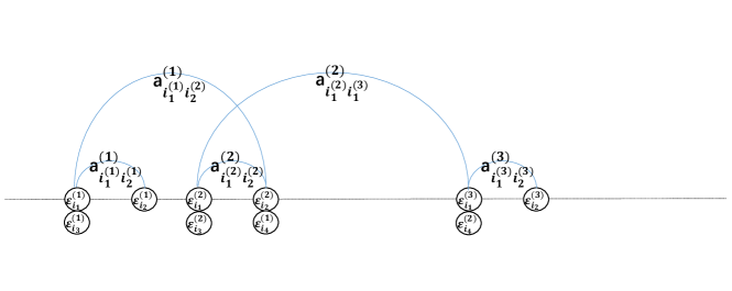
Figure 2. A graph associated with terms that satisfy $i_{1}^{(1)}$ equal to $i_{3}^{(1)}$, $i_{1}^{(2)}$ equal to $i_{3}^{(2)}$, $i_{2}^{(2)}$ equal to $i_{4}^{(1)}$ and $i_{1}^{(3)}$ equal to $i_{4}^{(2)}$.

We next classify all the terms in the above summation into three groups. Group one contains all the terms whose corresponding combined graph $G$ has at least one subgraph that does not have any vertices coincident with vertices of the other subgraphs. Group two contains all the terms whose corresponding combined graph $G$ has at least one vertex that is not coincident with any other vertices. All the other terms are classified into the third group. Since the entries in $\varepsilon$ are independent with 0 means, all the terms in group one and group two are equal to 0.

For example, for $q=4,k=5,k_{1}=2.k_{2}=2,k_{3}=1,k_{4}=0$, the term associated with the graph shown in Figure 2 is classified into group two, while the term associated with the graph shown in Figure 3 is classified into group one.

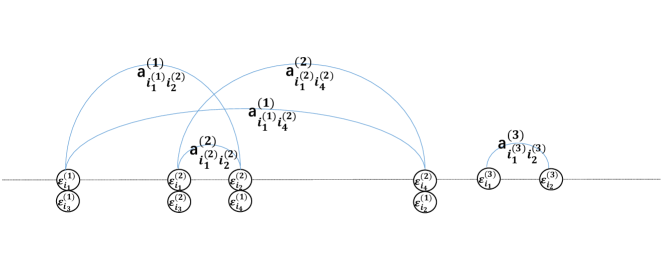
Figure 3. A graph associated with terms classified into group one.

Therefore, we need only to evaluate the sum of terms that belong to the third group. Suppose the combined graph $G$ contains $\pi$ connected pieces $\hat{G}_{1},\cdots,\hat{G}_{\pi}$ consisting of $\phi_{1},\cdots,\phi_{\pi}$ subgraphs ($G_{1},\cdots,G_{q}$). Clearly, $\phi_{1},\phi_{2},\cdots,\phi_{\pi}\geq 2$ since any subgraph must have at least one vertex coincident with vertices of the other subgraphs; hence, $\pi\leq k/2$ since $\phi_{1}+\cdots+\phi_{\pi}=k$. For example, in graph G shown in Figure 4, $q=4$, $k=8$, $\pi=2$, $\phi_{1}=\phi_{2}=4$.

Figure 4. A graph G associated with terms classified into group three.

We then introduce some necessary definitions and lemmas about graph-associated multiple matrices for the purpose of calculating the contributions of those terms in group three.

We first give two definitions:

Definition 4.2 (two-edge connected).

A graph $G$ is called two-edge connected if the resulting subgraph is still connected after removing any edge from G.

Definition 4.3 (cutting edge).

An edge $e$ in a graph $G$ is called a cutting edge if deleting this edge results in a disconnected subgraph.

Clearly, a graph is a two-edge connected graph if and only if there is no cutting edge. 5 below shows an example of a two-edge connected graph, while the graph show in Figure 6 is not a two-edge connected graph and has two cutting edges.

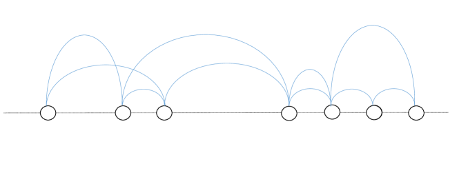
Figure 5. An example of a two-edge connected graph.

Figure 6. An example of graph that is not two-edge connected. There are two cutting edges.

Now, we shall introduce the following lemma.

Lemma 4.4.

Suppose that $\mathbf{G}=\left(\mathbf{V},\mathbf{E},\mathbf{F}\right)$ is a two-edge connected graph with $t$ vertices and $k$ edges. Each vertex $i$ corresponds to an integer $m_{i}\geq 2$, and each edge $e_{j}$ corresponds to a matrix $\mathbf{T}^{(j)}=\left(t_{\alpha,\beta}^{(j)}\right),\ j=1,\cdots,k$ with consistent dimensions, that is, if $F(e_{j})=(f_{i}(e_{j}),f_{e}(e_{j}))=(g,h),$ then the matrix $\mathbf{T}^{\left(j\right)}$ has dimensions $m_{g}\times m_{h}$. Define $\mathbf{v}=(v_{1},v_{2},\cdots,v_{t})$ and

(4.8) $$T^{\prime}=\sum_{\mathbf{v}}\prod_{j=1}^{k}t_{v_{f_{i}(e_{j})},v_{f_{e}(e_{j})}}^{(j)},$$

where the summation $\sum_{\mathbf{v}}$ is taken for $v_{i}=1,2,\cdots,m_{i},\ i=1,2,\cdots,t.$ Then, for any $i\leq t$, we have

$$|T^{\prime}|\leq m_{i}\prod_{j=1}^{k}\|\mathbf{T}^{(j)}\|.$$

For the proof of this lemma, we refer the reader to section $\mathbf{A}.4.2$ in [Bai and Silverstein(2010)].

Now, suppose that the connected piece $\hat{G}_{\varphi}$ ($1\leq\varphi\leq\pi$) consists of $\phi_{\varphi}$ subgraphs ($G_{1},\cdots,G_{q}$). Then, the number of edges in $\hat{G}_{\varphi}$ is exactly $\phi_{\varphi}$. Let $\upsilon_{\varphi}$ denote the number of noncoincident vertices (in graph G shown in Figure 4, $\upsilon_{1}=4,\upsilon_{2}=3$). Denote those vertices by $V_{\phi,1},\cdots,V_{\phi,\upsilon_{\varphi}}$. Additionally, denote the degree of those vertices by $\omega_{\phi,1},\cdots,\omega_{\phi,\upsilon_{\varphi}}$. Clearly, $\upsilon_{\varphi}\leq\phi_{\varphi}$ since the total degree is $2\phi_{\varphi}$ and the degrees of all vertices are at least 2.

Note that ${\rm E}\prod_{t=1}^{\phi_{\varphi}}(\mathbf{A}_{G_{\varphi t}}\boldsymbol{\varepsilon}_{G_{\varphi t}}-{\rm E}\mathbf{A}_{G_{\varphi t}}\boldsymbol{\varepsilon}_{G_{\varphi t}})=\mathbf{A}_{G_{\varphi}}{\rm E}\prod_{t=1}^{\phi_{\varphi}}(\boldsymbol{\varepsilon}_{G_{\varphi t}}-{\rm E}\boldsymbol{\varepsilon}_{G_{\varphi t}})$. We now focus on estimating the relationship between $\upsilon_{\varphi}$ and $\phi_{\varphi}$.

• Case (1): If $\upsilon_{\varphi}=\phi_{\varphi}$, then all the vertices in $\hat{G}_{\varphi}$ are of degree 2; thus, $\hat{G}_{\varphi}$ is an Euler graph, which is a circle and is therefore two-edge connected. It follows from Lemma 4.4 that $\sum_{\hat{G}_{\varphi}}\mathbf{A}_{\hat{G}_{\varphi}}=O(n).$ Since the fourth moment of the underlying distribution is finite, we have $|E\varepsilon_{\hat{G}_{\varphi}}|=O(1)$. An example of a graph in this case with $\phi_{\varphi}=8$ is shown in Figure 7.

  

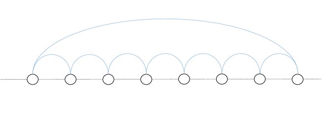
  Figure 7. An example of graph that falls into Case (1).

• Case (2): If there is exactly two vertices of degree 3 and all other vertices are of degree 2, then the two vertices of degree 3 must lie on the two “sides” of $\hat{G}_{\varphi}.$ There are two types of graphs that satisfy these conditions, as shown in Figure 8.

  

  Figure 8. Two types of graphs that fall into Case (2).

  All graphs of the second type are clearly two-edge connected. For the first type of graph, we have $\sum_{\hat{G}_{\varphi}}\mathbf{A}_{\hat{G}_{\varphi}}=\sum_{i,j=1}^{n}b_{i,j},$ where $\mathfrak{B}=(b_{i,j})_{n\times n}=\mathfrak{D_{1}}\mathfrak{A}\mathfrak{D_{2}}$ with $\mathfrak{D_{1}}$ and $\mathfrak{D_{2}}$ being diagonal matrices with a bounded spectrum norm. The above arguments imply that we also have $\sum_{\hat{G}_{\varphi}}\mathbf{A}_{\hat{G}_{\varphi}}=O(n)$ and $|E\varepsilon_{\hat{G}_{\varphi}}|=O(1)$.

• Case (3): If there is exactly one vertex of degree 4 and all other vertices are of degree 2, then, similarly to Case (1), we have $\sum_{\hat{G}_{\varphi}}\mathbf{A}_{\hat{G}_{\varphi}}=O(n).$ Moreover, we still have $|E\varepsilon_{\hat{G}_{\varphi}}|=O(1).$

• Case (4): $\hat{G}_{\varphi}$ is a graph that does not fall into the above three cases. Then, suppose there are $\kappa_{\varphi}$ vertices in $\hat{G}_{\varphi}$ with degrees larger than 4. Without loss of generality, denote these vertices as $\varrho_{\phi,1},\cdots,\varrho_{\phi,\kappa_{\varphi}}$. Choose a minimal spanning tree $\hat{G}_{\varphi}^{0}$ from $\hat{G}_{\varphi}$. Denote the remaining graph by $\hat{G}_{\varphi}^{1}$. An example graph $\hat{G}_{\varphi}$ that falls into this case is shown in Figure 9.

  

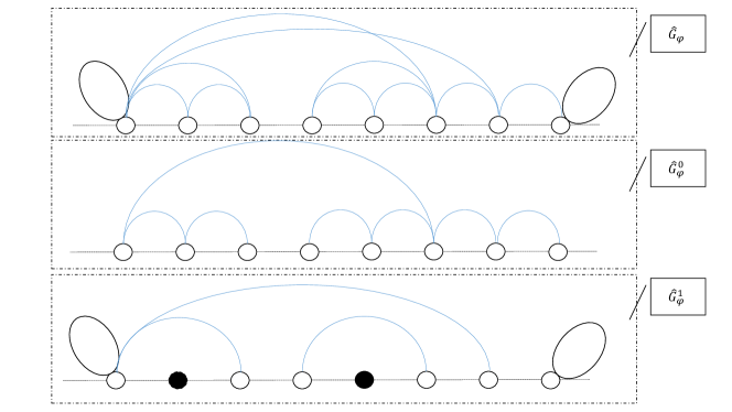
  Figure 9. An example graph $\hat{G}_{\varphi}$ that falls into Case (4). $\hat{G}_{\varphi}^{0}$ is a minimal spanning tree of $\hat{G}_{\varphi}$, and $\hat{G}_{\varphi}^{1}$ is the remaining graph.

  Then, by the Cauchy-Schwarz inequality, we have

  $$\sum_{\hat{G}_{\varphi}}\mathbf{A}_{\hat{G}_{\varphi}}\leq\left(\sum_{\hat{G}_{\varphi}}\mathbf{A}_{\hat{G}_{\varphi}^{0}\cup\hat{G}_{\varphi}^{0}}\right)^{1/2}\left(\sum_{\hat{G}_{\varphi}}\mathbf{A}_{\hat{G}_{\varphi}^{1}\cup\hat{G}_{\varphi}^{1}}\right)^{1/2}.$$

  Note that all the degrees of the vertices in ${\hat{G}_{\varphi}^{0}\cup\hat{G}_{\varphi}^{0}}$ are even; thus, ${\hat{G}_{\varphi}^{0}\cup\hat{G}_{\varphi}^{0}}$ is an Euler graph. Additionally, note that $\hat{G}_{\varphi}^{0}$ contains all the vertices of $\hat{G}_{\varphi}$. It follows from Lemma 4.4 that $\sum_{\hat{G}_{\varphi}}\mathbf{A}_{\hat{G}_{\varphi}^{0}\cup\hat{G}_{\varphi}^{0}}=O(n).$ For the same reason, since all the degrees of the vertices in ${\hat{G}_{\varphi}^{1}\cup\hat{G}_{\varphi}^{1}}$ are even and the number of disconnected subgraphs (including isolated vertices, if they exist) of ${\hat{G}_{\varphi}^{1}\cup\hat{G}_{\varphi}^{1}}$ is at most $\upsilon_{\varphi}$. Thus, we have $\sum_{\hat{G}_{\varphi}}\mathbf{A}_{\hat{G}_{\varphi}^{0}\cup\hat{G}_{\varphi}^{0}}=O(n^{\upsilon_{\varphi}}).$ Now, we estimate $|E\varepsilon_{\hat{G}_{\varphi}}|.$ If $\kappa_{\varphi}=0,$ then we have $|E\varepsilon_{\hat{G}_{\varphi}}|=O(1).$ If $\kappa_{\varphi}\geq 1,$ denote the degrees of $\varrho_{\phi,1},\cdots,\varrho_{\phi,\kappa_{\varphi}}$ as $d_{\varrho_{\phi,1}},\cdots,d_{\varrho_{\phi,\kappa_{\varphi}}}$, respectively. Since the underlying variables are truncated and $\delta_{n}\to 0$, we obtain that, for large $n$,

  (4.9) $$|E\varepsilon_{\hat{G}_{\varphi}}|\leq\left(\delta_{n}n^{1/4}\right)^{\left(\sum_{i=1}^{\kappa_{\varphi}}\left(d_{\varrho_{\phi,i}}-4\right)\right)}=o\left(n^{\frac{\sum_{i=1}^{\kappa_{\varphi}}\left(d_{\varrho_{\phi,i}}-4\right)}{4}}\right),$$

  which implies that

  (4.10) $$\mathbf{A}_{\hat{G}_{\varphi}}{\rm E}\prod_{t=1}^{\phi_{\varphi}}(\boldsymbol{\varepsilon}_{\hat{G}_{\varphi t}}-{\rm E}\boldsymbol{\varepsilon}_{\hat{G}_{\varphi t}})=o(n^{1/2}n^{{\upsilon_{\varphi}}/2}n^{\frac{\sum_{i=1}^{\kappa_{\varphi}}\left(d_{\varrho_{\phi,i}}-4\right)}{4}})=o(n^{\frac{{\sum_{i=1}^{\kappa_{\varphi}}d_{\varrho_{\phi,i}}}-4\kappa_{\varphi}+2\upsilon_{\varphi}+2}{4}})$$

  $$= o\left(n^{{\frac{{\sum_{i=1}^{\kappa_{\varphi}}d_{\varrho_{\phi,i}}}+2\left(\upsilon_{\varphi}-\kappa_{\varphi}\right)-2\kappa_{\varphi}+2}{4}}}\right)=o(n^{\frac{\phi_{\varphi}}{2}}),$$

  since ${{{\sum_{i=1}^{\kappa_{\varphi}}d_{\varrho_{\phi,i}}}+2\left(\upsilon_{\varphi}-\kappa_{\varphi}\right)}}\leq 2{\phi_{\varphi}}$ and $\kappa_{\varphi}\geq 1.$

We have now established the following lemma.

Lemma 4.5.

For the $\varphi$-th connected graph ${\hat{G}_{\varphi}}$, if $\phi_{\varphi}>2$, then

(4.11) $$\sum_{\hat{G}_{\varphi}}{\rm E}\prod_{t=1}^{\phi_{\varphi}}(\mathbf{\mathbf{A}}_{\hat{G}_{\varphi t}}\boldsymbol{\varepsilon}_{\hat{G}_{\varphi t}}-{\rm E}\mathbf{\mathbf{A}}_{\hat{G}_{\varphi t}}\boldsymbol{\varepsilon}_{\hat{G}_{\varphi t}})=o(n^{\phi_{\varphi}/2}),$$

and if $\phi_{\varphi}=2$, then

(4.12) $$\sum_{\hat{G}_{\varphi}}{\rm E}\prod_{t=1}^{\phi_{\varphi}}(\mathbf{\mathbf{A}}_{\hat{G}_{\varphi t}}\boldsymbol{\varepsilon}_{\hat{G}_{\varphi t}}-{\rm E}\mathbf{\mathbf{A}}_{\hat{G}_{\varphi t}}\boldsymbol{\varepsilon}_{\hat{G}_{\varphi t}})=O(n^{\phi_{\varphi}/2})=O(n).$$

Now, we return to the proof of the joint central limit theorem.

We have the following facts:

(i) when $k$ is odd:

Applying Lemma 4.5, if $k$ is odd, since for any $G$ there are at least two connected subgraphs of $G$ that contain more than two constructing basic graphs, the second conclusion of (4.4) holds.

(ii) when $k$ is even:

When $k$ is even, $G$ consists of $u_{i,j}$ ($1\leq i,j\leq q$) connected subgraphs composed of two basic graphs $G_{i}$ if $i=j$ and one basic graph $G_{i}$ and one basic graph $G_{j}$ if $j\neq i$. Clearly, we have $2u_{i,i}+\sum_{j\neq i}u_{i,j}=k_{i}$ and $u_{i,j}=u_{j,i}$. Compare

(4.13) $$\sum_{G}{\rm E}\left(\prod_{l=1}^{q}\prod_{\ell=1}^{k_{l}}(A_{G_{l,\ell}}\varepsilon_{{G_{l},\ell}}-{\rm E}A_{G_{l,\ell}}\varepsilon_{{G_{l,\ell}}})\right)$$

with the expansion of

(4.14) $$\prod_{1\leq i\leq j\leq q}\left({\rm Cov(Q_{i},Q_{j})}\right)^{u_{i,j}}= (E(Q_{1}-EQ_{1})^{2})^{u_{1,1}}(E(Q_{2}-EQ_{2})^{2})^{u_{2,2}}\cdots(E(Q_{q}-EQ_{q}))^{u_{q,q}}$$

$$\times (E(Q_{1}-EQ_{1})E(Q_{2}-EQ_{2}))^{u_{1,2}}\cdots(E(Q_{1}-EQ_{1})E(Q_{q}-EQ_{q}))^{u_{1,q}}$$

$$\vdots$$

$$\times (E(Q_{q-1}-EQ_{q-1})E(Q_{q}-EQ_{q}))^{u_{q-1,q}}.$$

The latter expansion (4.14) contains more terms than (4.13), with more connections among the subgraphs. For the readers’ convenience, in Figure 10, we give an example where the term corresponding to $\hat{G}_{(1)}$ belongs to both (4.14) and (4.13) while the term corresponding to $\hat{G}_{(2)}$ belongs to (4.14) but not to (4.13).

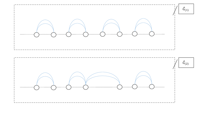
Figure 10. An example of ${\hat{G}_{(1)}}$ and ${\hat{G}_{(2)}}$.

Therefore, for the same reason as the arguments above, we know that the whole contribution of the difference terms between (4.14) and (4.13) has an order of $o(n^{k/2})$; thus,

(4.15) $$\sum_{G}{\rm E}\left(\prod_{l=1}^{q}\prod_{\ell=1}^{k_{l}}(A_{G_{l,\ell}}\varepsilon_{{G_{l},\ell}}-{\rm E}A_{G_{l,\ell}}\varepsilon_{{G_{l,\ell}}})\right)=\prod_{1\leq i\leq j\leq q}\left({\rm Cov(Q_{i},Q_{j})}\right)^{u_{i,j}}+o(n^{k/2}).$$

Therefore, we obtain

(4.16) $${\rm E}\prod_{l=1}^{q}(Q_{l}-{\rm E}Q_{l})^{k_{l}}=\sum_{\begin{subarray}{c}2u_{1,1}+\sum_{j\neq 1}u_{1,j}=k_{1}\\ \vdots\\ 2u_{q,q}+\sum_{j\neq q}u_{q,j}=k_{q}\end{subarray}}\frac{k!}{2^{\sum_{l=1}^{q}u_{l,l}}\prod_{1\leq i\leq j\leq q}u_{i,j}!}\prod_{1\leq i\leq j\leq q}\left({\rm Cov(Q_{i},Q_{j})}\right)^{u_{i,j}}+o(n^{k/2}).$$

Substituting (4.16) into (4.5) yields

(4.17) $${\rm E}\left(\sum_{l=1}^{q}\alpha_{l}\left(Q_{l}-{\rm E}Q_{l}\right)\right)^{k}$$

$$= \sum_{\sum_{1\leq i\leq j\leq q}u_{i,j}=k}\frac{k!}{2^{\sum_{l=1}^{q}u_{l,l}}\prod_{1\leq i\leq j\leq q}u_{i,j}!}\prod_{l=1}^{q}\alpha_{l}^{2u_{l,l}+\sum_{j\neq l}u_{l,j}}\prod_{1\leq i\leq j\leq q}\left({\rm Cov(Q_{i},Q_{j})}\right)^{u_{i,j}}+o(n^{k/2})$$

$$= \frac{k!}{2^{k/2}(k/2)!}\left(\sum_{i=1}^{q}\sum_{j=1}^{q}\alpha_{i}\alpha_{j}{\rm Cov}\left(Q_{i},Q_{j}\right)\right)^{k/2}+o(n^{k/2})$$

$$= (k-1)!!\left(\sum_{l_{1}=1}^{q}\sum_{l_{2}=1}^{q}\alpha_{l_{1}}\alpha_{l_{2}}{\rm Cov}\left(Q_{l_{1}},Q_{l_{2}}\right)\right)^{k/2}+o(n^{k/2}).$$

Since we assume that there exists an $i$ such that ${\rm Cov}(Q_{i},Q_{i})$ has the same order as $n$, we conclude that for almost all $(\alpha_{1},\alpha_{2},\cdots,\alpha_{q})\in\mathbb{R}^{q}$, we have that

$$\left(\sum_{l_{1}=1}^{q}\sum_{l_{2}=1}^{q}\alpha_{l_{1}}\alpha_{l_{2}}{\rm Cov}\left(Q_{l_{1}},Q_{l_{2}}\right)\right)$$

has the same order as $n$. In fact, note that $n^{-1}\left(\sum_{l_{1}=1}^{q}\sum_{l_{2}=1}^{q}\alpha_{l_{1}}\alpha_{l_{2}}{\rm Cov}\left(Q_{l_{1}},Q_{l_{2}}\right)\right)$, and $f(\alpha_{1},\alpha_{2},\cdots,\alpha_{q})$ is a polynomial in variables $\alpha_{1},\alpha_{2},\cdots,\alpha_{q}.$ We know from the fundamental properties of polynomials that one and exactly one of the following two cases holds: (1) The polynomials $f(\alpha_{1},\alpha_{2},\cdots,\alpha_{q})\equiv 0$ for all vector $\left(\alpha_{1},\alpha_{2},\cdots,\alpha_{q}\right)$. (2) The Lebesgue measure of the set of vectors $\left(\alpha_{1},\alpha_{2},\cdots,\alpha_{q}\right)$ in the space $\mathbb{R}^{q}$ such that polynomials $f(\alpha_{1},\alpha_{2},\cdots,\alpha_{q})=0$ is zero. We thus obtain the conclusion since (1) conflicts with our assumption by taking $\alpha_{i}=1$ and $\alpha_{j}=0$ for $j\neq i$.

Finally, by applying the moment convergence theorem and continuity, we arrive at the fact that for all $\left(\alpha_{1},\alpha_{2},\cdots,\alpha_{q}\right)$,

$$\sqrt{1/n}\left(\sum_{l=1}^{q}\alpha_{l}\left(Q_{l}-{\rm E}Q_{l}\right)\right)\stackrel{{\scriptstyle\mathcal{D}}}{{\sim}}N(0,\frac{\left(\sum_{l_{1}=1}^{q}\sum_{l_{2}=1}^{q}\alpha_{l_{1}}\alpha_{l_{2}}{\rm Cov}\left(Q_{l_{1}},Q_{l_{2}}\right)\right)}{n}).$$

The proof of Theorem 4.1 is complete.

5. Conclusion and further discussion

In this paper, we consider tests for detecting series correlation that are valid in both low- and high-dimensional linear regression models with random and fixed designs. The test statistics are based on the residuals of OLS and the residual maker matrix. We need no model assumptions on the regressor and/or dependent variable; thus, the tests are model-free. The asymptotic distribution of the statistics under the null hypothesis are obtained as a consequence of a general joint CLT of quadratic forms. Simulations are conducted to investigate the advantages of the proposed test procedures. The results show that the proposed tests perform well if $n-p$, where $n$ is the sample size and $p$ is the number of regressors, is not too small.

If we are concerned about the robustness, then we can use the standard residuals $\check{\varepsilon}_{j}=\varepsilon_{j}/\sqrt{p_{jj}}$ $1\leq j\leq n$ instead of the original residuals. Then, the residual vector can be rewritten as $\check{\boldsymbol{\varepsilon}}=(\check{\varepsilon}_{1},\ldots,\check{\varepsilon}_{n})^{\prime}=\mathbf{D}\mathbf{R}\mathbf{\Sigma}^{1/2}\boldsymbol{\epsilon}$, where $\mathbf{D}$ is a diagonal matrix with diagonal entries $\{r_{jj}^{-1/2}\}_{j=1}^{n}$. Then, the test procedures remain valid after recalculating $m_{\tau}$ for $0\leq\tau\leq q$ and $v_{\tau_{1}\tau_{2}}$ for $0\leq\tau_{1},\tau_{2}\leq q$ by replacing $\mathbf{R}$ with $\mathbf{D}\mathbf{R}$ in (2.1) and (2.2).

References

- [Al-Naffouri et al.(2016)Al-Naffouri, Moinuddin, Ajeeb, Hassibi, and Moustakas] Tareq Y. Al-Naffouri, Muhammad Moinuddin, Nizar Ajeeb, Babak Hassibi, and Aris L. Moustakas. On the distribution of indefinite quadratic forms in gaussian random variables. IEEE Transactions on Communications, 64(1):153–165, 2016.
- [Azzalini and Bowman(1993)] Adelchi Azzalini and Adrian Bowman. On the use of nonparametric regression for checking linear relationships. Journal of the Royal Statistical Society. Series B (Methodological), 55(2):549–557, 1993.
- [Bai and Silverstein(2010)] Zhi Dong Bai and Jack William Silverstein. Spectral analysis of large dimensional random matrices. Springer, 2010.
- [Bai et al.(2018)Bai, Pan, and Yin] Zhidong Bai, Guangming Pan, and Yanqing Yin. A central limit theorem for sums of functions of residuals in a high-dimensional regression model with an application to variance homoscedasticity test. TEST, 27(4):896–920, Dec 2018. ISSN 1863-8260. doi: 10.1007/s11749-017-0575-x. URL https://doi.org/10.1007/s11749-017-0575-x.
- [Bartlett et al.(1960)Bartlett, Gower, and Leslie] M. S. Bartlett, J. C. Gower, and P. H. Leslie. The characteristic function of hermitian quadratic forms in complex normal variables. Biometrika, 47(1/2):199–201, 1960.
- [Bercu and Proia(2013)] Bernard Bercu and Frederic Proia. A sharp analysis on the asymptotic behavior of the durbin-watson for the first-order autoregressive process. ESAIM - Probability and Statistics, 17(1):500–530, 2013.
- [Box and Pierce(1970)] George EP Box and David A Pierce. Distribution of residual autocorrelations in autoregressive-integrated moving average time series models. Journal of the American statistical Association, 65(332):1509–1526, 1970.
- [Breusch and Pagan(1979)] Trevor S Breusch and Adrian R Pagan. A simple test for heteroscedasticity and random coefficient variation. Econometrica: Journal of the Econometric Society, 47(5):1287–1294, 1979.
- [Cambanis et al.(1985)Cambanis, Rosinski, and Woyczynski] Stamatis Cambanis, Jan Rosinski, and Wojbor A. Woyczynski. Convergence of quadratic forms in p-stable random variables and θp-radonifying operators. Annals of Probability, 13(3):885–897, 1985.
- [Cook and Weisberg(1983)] R Dennis Cook and Sanford Weisberg. Diagnostics for heteroscedasticity in regression. Biometrika, 70(1):1–10, 1983.
- [Darroch(1961)] J. N. Darroch. Computing the distribution of quadratic forms in normal variables. Biometrika, 49(3-4):109–15, 1961.
- [de Jong(1987)] Peter de Jong. A central limit theorem for generalized quadratic forms. Probability Theory and Related Fields, 75(2):261–277, 1987.
- [Dette and Munk(1998)] Holger Dette and Axel Munk. Testing heteroscedasticity in nonparametric regression. Journal of the Royal Statistical Society: Series B (Statistical Methodology), 60(4):693–708, 1998.
- [Deya and Nourdin(2014)] Aurélien Deya and Ivan Nourdin. Invariance principles for homogeneous sums of free random variables. Bernoulli, 20(2):586–603, 2014.
- [Dik and De Gunst(2010)] J. J Dik and M. C. M De Gunst. The distribution of general quadratic forms in normal variables. Statistica Neerlandica, 39(1):14–26, 2010.
- [Durbin(1970)] J. Durbin. Testing for serial correlation in least-squares regression when some of the regressors are lagged dependent variables. Econometrica, 38(3):410–421, 1970.
- [Durbin and Watson(1950)] James Durbin and Geoffrey S Watson. Testing for serial correlation in least squares regression: I. Biometrika, 37(3/4):409–428, 1950.
- [Durbin and Watson(1951)] James Durbin and Geoffrey S Watson. Testing for serial correlation in least squares regression. ii. Biometrika, 38(1/2):159–177, 1951.
- [Durbin and Watson(1971)] James Durbin and Geoffrey S Watson. Testing for serial correlation in least squares regression. iii. Biometrika, 58(1):1–19, 1971.
- [Forchini(2002)] G. Forchini. The exact cumulative distribution function of a ratio of quadratic forms in normal variables, with application to the ar(1) model. Econometric Theory, 18(4):823–852, 2002.
- [Fox and Taqqu(1985)] Robert Fox and Murad S. Taqqu. Central limit theorems for quadratic forms in random variables having long-range dependence. Annals of Probability, 13(2):428–446, 1985.
- [Gart(1970)] John J. Gart. Notes on the distribution of quadratic forms in singular normal variables. Biometrika, 57(3):567–572, 1970.
- [Gençay and Signori(2015)] Ramazan Gençay and Daniele Signori. Multi-scale tests for serial correlation. Journal of Econometrics, 184(1):62–80, 2015.
- [Glejser(1969)] Herbert Glejser. A new test for heteroskedasticity. Journal of the American Statistical Association, 64(325):316–323, 1969.
- [Gotze and Tikhomirov(1999)] F Gotze and Aleksandr N Tikhomirov. Asymptotic distribution of quadratic forms. Annals of probability, 27(2):1072–1098, 1999.
- [Gregory and Hughes(1995)] J Gregory and H. R. Hughes. Random quadratic forms. Transactions of the American Mathematical Society, 347(2):709–717, 1995.
- [Harrison and McCabe(1979)] Michael J Harrison and Brendan PM McCabe. A test for heteroscedasticity based on ordinary least squares residuals. Journal of the American Statistical Association, 74(366a):494–499, 1979.
- [Hsu et al.(1999)Hsu, Prentice, Zhao, and Fan] L. Hsu, R. L. Prentice, L. P. Zhao, and J. J. Fan. Miscellanea. saddlepoint approximations for distributions of quadratic forms in normal variables. Biometrika, 86(4):929–935, 1999.
- [Inder(1986)] Brett Inder. An approximation to the null distribution of the durbin-watson statistic in models containing lagged dependent variables. Econometric Theory, 2(3):413–428, 1986.
- [King and Wu(1991)] Maxwell L King and Ping X Wu. Small-disturbance asymptotics and the durbin-watson and related tests in the dynamic regression model. Journal of Econometrics, 47(1):145–152, 1991.
- [Li and Gençay(2017)] Meiyu Li and Ramazan Gençay. Tests for serial correlation of unknown form in dynamic least squares regression with wavelets ☆. Economics Letters, 155:104–110, 2017.
- [Li and Yao(2015)] Zhaoyuan Li and Jianfeng Yao. Homoscedasticity tests valid in both low and high-dimensional regressions. arXiv preprint arXiv:1510.00097, 2015.
- [Liu et al.(2009)Liu, Tang, and Zhang] Huan Liu, Yongqiang Tang, and Hao Helen Zhang. A new chi-square approximation to the distribution of non-negative definite quadratic forms in non-central normal variables. Computational Statistics & Data Analysis, 53(4):853–856, 2009.
- [Ljung and Box(1978)] Greta M Ljung and George EP Box. On a measure of lack of fit in time series models. Biometrika, 65(2):297–303, 1978.
- [Nerlove and Wallis(1966)] Marc Nerlove and Kenneth F. Wallis. Use of the durbin-watson statistic in inappropriate situations. Econometrica, 34(1):235–238, 1966.
- [Oliveira(2016)] Roberto Imbuzeiro Oliveira. The lower tail of random quadratic forms with applications to ordinary least squares. Probability Theory & Related Fields, 166(3-4):1–20, 2016.
- [Stocker(2007)] Toni Stocker. On the asymptotic bias of ols in dynamic regression models with autocorrelated errors. Statistical Papers, 48(1):81–93, 2007.
- [White(1980)] Halbert White. A heteroskedasticity-consistent covariance matrix estimator and a direct test for heteroskedasticity. Econometrica: Journal of the Econometric Society, 48(4):817–838, 1980.