Disentangling Video with Independent Prediction

Abstract

We propose an unsupervised variational model for disentangling video into independent factors, i.e. each factor’s future can be predicted from its past without considering the others. We show that our approach often learns factors which are interpretable as objects in a scene.

1 Introduction

Deep neural networks have delivered impressive performance on a range of perceptual tasks, but their distributed representation is difficult to interpret and poses a challenge for problems involving reasoning. Motivated by this, the deep learning community has recently explored methods [1–4,6–8,12,15–17,20,21] for learning distributed representations which are disentangled, i.e. a unit (or small group) within the latent feature vector are exclusively responsible for capturing distinct concepts within the input signal. This work proposes such an approach for the video domain, where the temporal structure of the signal is leveraged to automatically separate the input into factors that vary independently of one another over time. Our results demonstrate that these factors correspond to distinct objects within the video, thus providing a natural representation for making predictions about future motions of the objects and subsequent high-level reasoning tasks.

Related work. [22] leverage structure at different time-scales to factor signals into independent components. Our approach can handle multiple factors at the same time-scale, instead relying on prediction as the factoring mechanism. Outside of the video domain, [1] proposed to disentangle factors that tend to change independently and sparsely in real-world inputs, while preserving information about them. [15] learned to disentangle factors of variation in synthetic images using weak supervision, and [21] extended the method to be fully unsupervised. Similar to our work, both [3] and [4] propose unsupervised schemes for disentangling video, the latter using a variational approach. However, ours differs in that it uncovers general factors, rather than specific ones like identity and pose or static/dynamic features as these approaches do.

2 Generative model and inference

The intuition behind our model is simple: in any real-world scene, most objects do not physically interact with one another, so their motion can be modeled independently. To find a representation of videos with these same independences, we introduce an approach based on a temporal version [14] of the variational auto-encoder [10], shown in Figure 1. In this model, each video $X$ comprises a sequence of frames $x_{1}...x_{n}$. $Z_{t}=z^{1}_{t}...z^{k}_{t}$ represents all the latent factors at time $t$, where each factor $z^{i}_{t}$ is represented by a vector. Each of these factors evolve independently from one another and combine to produce the observation $x_{t}$ for timestep $t$. Instead of directly maximizing the likelihood $p(X;\theta)$, we use variational inference [5] to optimize the evidence lower bound (ELBO), that is $\theta^{*},\phi^{*}=\operatorname*{arg\,max}_{\theta,\phi}\mathcal{L}(\theta,\phi;X):$

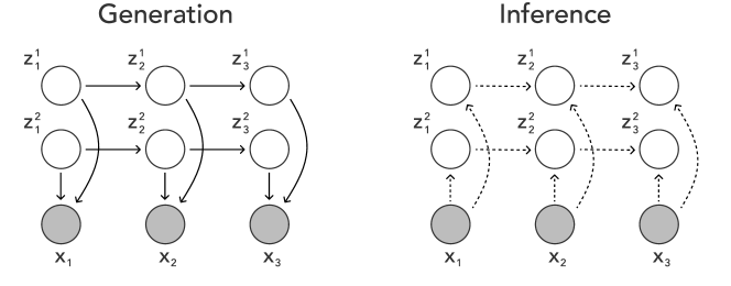
Figure 1: Left: Our generative model. Several latent variables combine to produce each observation, and each variable evolves through time independently of the others, just like objects which do not collide. Each observation $x_{t}$ is given by a decoder which produces $p_{\theta}(x_{t}|z^{1}_{t}...z^{k}_{t})$. Right: Our variational inference procedure gives $q_{\phi}(z^{1}_{t}...z^{k}_{t}|x_{t},z^{1}_{t-1}...z^{k}_{t-1})\approx p(z^{1}_{t}...z^{k}_{t}|x_{t},z^{1}_{t-1}...z^{k}_{t-1})$.

$$\operatorname*{\scalerel*{\mathbb{E}}{\textstyle\sum}}_{Z\sim q_{\phi}(Z|X)}\log p_{\theta}(X|Z)\\ -D_{KL}(q_{\phi}(Z_{1}|X)||p_{\theta}(Z_{1}))\ -\sum_{t=2}^{n}\operatorname*{\scalerel*{\mathbb{E}}{\textstyle\sum}}_{\begin{subarray}{c}Z_{t-1}\sim\\ q(Z_{t-1}|Z_{t-2},X)\end{subarray}}\ D_{KL}(q_{\phi}(Z_{t}|Z_{t-1},X)||p_{\theta}(Z_{t}|Z_{t-1}))$$

For a derivation, see Appendix B. This lower bound naturally splits into two factors. The first, $p_{\theta}(X|Z)$, is the log-likelihood of the data $X$ under our model when sampling from the approximate posterior, that is the “reconstruction” of $X$ from $Z$. The second factor is the KL divergence between the learned prior $p_{\theta}(Z)$ and the approximate posterior $q_{\phi}(Z|X)$. It represents how far the predictions given by $p$ are from the inferred values given by $q$; it is the prediction error in the latent space. Our goal is to optimize the space of Z to make both reconstruction and prediction possible.

For the variational approximation, we choose $q_{\phi}(Z|X)=\prod_{t=1}^{n}q(Z_{t}|Z_{t-1},x_{t};\phi)$ which, analogous to a Kalman filter, considers only the past state and current observation. This approximation marginalizes over the future, in that $q(Z_{t}|Z_{t-1},x_{t})$ must encode sufficient information to allow correct predictions of the future as well as fit the prior and the current observation. This allows us to do inference on a single frame and ensure our representation retains as much information about the future as possible. If we wish to use our learned representation for a downstream task, we may discard the generative model and use the inference network alone. This inference network can provide a factorized representation given a single image or use a sequence of images to produce increasingly tight estimates of the latent variables.

Neural network parameterization. We choose all of the distributions in our model to be Gaussian with diagonal covariance. To allow our model to scale to complex nonlinear observations and dynamics, we parameterize each distribution with a neural network. Table 1 describes each of these parameterizations. As each distribution is diagonal Gaussian, each network produces two outputs, corresponding to the mean and the variance of each distribution.

Training. This model can be thought of as a series of variational autoencoders with a learned prior, and the training procedure is largely similar to [10]. At each timestep $t$ in a sequence, we compute the prior $p_{\theta}(Z_{t}|Z_{t-1})$ over the latent space, using $\mathcal{N}(0,\mathbb{I})$ for $t=0$. We infer the approximate posterior $q_{\phi}(Z_{t}|Z_{t-1},x_{t})$ by observing $x_{t}$ and compute the KL divergence $D_{KL}(q||p)$. We then sample $Z_{t}\sim q_{\phi}(Z_{t}|Z_{t-1},x_{t})$ using the reparameterization trick and compute $\log p_{\theta}(x_{t}|Z_{t})$. At the end of a sequence we update our parameters $\theta,\phi$ by backprop to maximize the ELBO (defined above).

distribution	parameterization	parameter sharing?
$p_{\theta}(z^{i}_{1})$	$\mathcal{N}(0,\mathbb{I})$	N/A (but same for each $i$)
$p_{\theta}(z^{i}_{t}|z^{i}_{t-1})$	MLP$(d\to 128,128\to 128,128\to d)$	across $t$ (different params for each $i$)
$p_{\theta}(x_{t}|Z_{t})$	DCGAN generator	across $t$
$q_{\phi}(Z_{t}|Z_{t-1},x_{t})$	DCGAN discriminator	across $t$

Table 1: The parameterization for each of the distributions in our model. Each latent factor has its own transition function, but all modules are shared across all timesteps. The variable $d$ is the dimension of the entire latent space including all factors. DCGAN refers to the architecture used in [14]. For more details, please see Appendix A.

3 Experiments

Datasets. We apply this model to two video datasets: the widely-used moving MNIST [19] and a new dataset of real-world videos of 5th Avenue recorded from above, which was collected by the authors. More details about these datasets, including a sample frame from 5th Avenue, can be found in Appendix C.

Baseline. In each of these evaluations we compare with a model which is identical to the factored model except that its transition function $p(Z_{t}|Z_{t-1})$ is not factored (referred to as the entangled model in our experiments). It can be viewed as a special case of our factored model which has a single high-dimensional latent factor, and its latent space has the same total dimension as the corresponding factored model in each experiment. This comparison is intended to be as tight as possible, with any differences between the factored model and the baseline coming exclusively from the factorization in the latent space.

3.1 Evaluation

Lower bound. We compare the variational lower bound achieved by our factorized model with that of a non-factorized but otherwise identical model. These experiments reveal the price in terms of data fidelity that we pay for representing the data as independently-changing factors. Table 2 shows that the factored model achieves a lower bound on par with the entangled model.

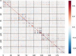
(a) Factored model

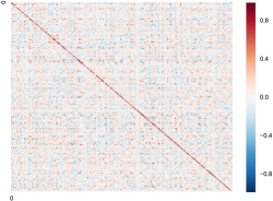
(b) Entangled model

Figure 2: Heatmap of correlation between latent variables (shown as blocks) at time $t$ (y-axis) vs. at time $t+1$ (x-axis) on the 5th Avenue dataset. The block-diagonal structure exhibited here reflects that $z^{i}_{t+1}$ largely depends on its own previous state $z^{i}_{t}$ rather than on the other latent factors. The entangled model does not appear to have structure in its latent space. These plots were generated using models with two-layer transition networks; with deeper transitions there is almost zero linear dependence between any pair of latent units.

Correlation structure. By plotting the correlation between samples from the approximate posterior over the latent variables at time $t$ and at time $t+1$, we may observe whether our model has been able to learn a representation for which $z^{i}_{t+1}$ really does only depend on $z^{i}_{t}$ and not on the other latent factors. Note that this only captures the linear dependence of these variables; this analysis helps to illustrate the structure of our latent space, but should not be considered definitive. Figure 2 shows that each latent factor is much more correlated with its own previous state than with other latent factors.

dataset, model	$\tilde{\mathbb{I}}(z^{i}_{t+1};z^{i}_{t})$	$\tilde{\mathbb{I}}(z^{i}_{t+1};z^{j\neq i}_{t})$	ELBO
moving MNIST, two factors	4.61	0.75	-2902
moving MNIST, entangled	4.66	2.61	-2896
5th Ave, eight factors	2.26	0.28	6830
5th Ave, entangled	2.08	0.38	6800

Table 2: Mutual information estimates and ELBO. In the factored model, the previous value of the same latent variable is substantially more predictive of its current value than are the previous values of any other variables. This shows that our model is actually factorizing. See Sec. 2 for details. The ELBO $\mathcal{L}(\theta,\phi;X)$ shows that our model pays a small or nonexistent price for factoring the latent space into independently-evolving components.

Approximate mutual information. We use Kraskov’s method for estimating mutual information [13] to approximate $\mathbb{I}(z^{i}_{t+1};z^{i}_{t})$ and compare it to $\mathbb{I}(z^{i}_{t+1};z^{j\neq i}_{t})$. A latent factor $z^{i}_{t}$ should be much more informative about its own future $z^{i}_{t+1}$ than a different factor $z^{j\neq i}_{t}$ is. The results, shown in Table 2, reveal that the evolution of each factor in the factored models depends almost exclusively on their past.

For the entangled models, which do not have separate factors, there is no a priori subdivision into high- and low-mutual-information segments of units. The reported scores were generated by creating 20 random partitionings of the latent units into $k$ factors, then reporting the mutual information numbers for the partitioning that had the greatest difference between same-factor and cross-factor information.

The entangled models show much more cross-factor information than the factored models in our tests on moving MNIST, where we use two latent factors. However, as the number of factors increases, the average information between a pair of factors naturally diminishes. As a result on 5th Avenue, where we subdivide the latent units into eight factors, the entangled model shows cross-information almost as low as the factored model.

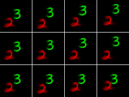
(a) Factorized reconstruction of moving MNIST

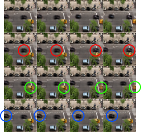
(b) Factorized reconstruction of 5th Avenue

Figure 3: Left, top row: reconstruction of the input sequence using all factors. Left, middle row: reconstructing the sequence varying only the first latent factor (of two). Only the green three moves, showing that factor 1 exactly represents the green digit. Left, bottom row: reconstructing the sequence varying only the second latent factor. Evolving factor two only affects the pose of the red digit. Right, top row: reconstruction of the input sequence using all latents. Right, other rows: reconstructions only varying a single latent factor. Several factors correspond to moving a single car in the image. Note that in the last row, the model removes the top-right black car; since the top-left car is moving forward quickly, it predicts that there must not be an obstacle in its way.

Independent generations. Finally, we evaluate qualitatively the representations learned by our model. We infer the approximate posterior $q(Z|X)$, then set all of the latent variables fixed at their $t=2$ values given by $q(Z_{2}|x_{1,2})$. We then produce a sequence of generations by picking a single variable $z^{i}$ to vary, then for each timestep $t=2...n$ drawing a sample from $p(x|z^{1}_{2}...z^{i-1}_{2},\boldsymbol{z^{i}_{t}},z^{i+1}_{2}...z^{k}_{2})$ (note the single bolded factor $\boldsymbol{z^{i}_{t}}$ varying with $t$). That is, we hold all but one of the latent variables fixed and allow the single one to vary with the posterior. This allows us to see exactly what that single variable represents in this video. The images generated by this process are shown in Figure 3.

4 Discussion

By taking advantage of the structure present in video, our model can pull apart latent factors which change independently and produce a representation composed of semantically meaningful variables. The approach is conceptually simple and based on the insight that if two objects do not interact, they can be predicted independently. In the future we hope to apply a richer family of approximations to scale to more complex data.

References

[1] Yoshua Bengio, Aaron Courville, and Pascal Vincent. 2013. Representation learning: A review and new perspectives. Pattern Analysis and Machine Intelligence, IEEE Transactions on 35, 8 (2013), 1798–1828.

[2] Michael B Chang, Tomer Ullman, Antonio Torralba, and Joshua B Tenenbaum. 2016. A compositional object-based approach to learning physical dynamics. arXiv preprint arXiv:1612.00341 (2016).

[3] Emily Denton and Vighnesh Birodkar. 2017. Unsupervised learning of disentangled representations from video. CoRR abs/1705.10915, (2017).

[4] Will Grathwohl and Aaron Wilson. 2016. Disentangling space and time in video with hierarchical variational auto-encoders. arXiv preprint arXiv:1612.04440 (2016).

[5] Matthew D Hoffman, David M Blei, Chong Wang, and John Paisley. 2013. Stochastic variational inference. The Journal of Machine Learning Research 14, 1 (2013), 1303–1347.

[6] Wei-Ning Hsu, Yu Zhang, and James R. Glass. 2017. Unsupervised learning of disentangled and interpretable representations from sequential data. CoRR abs/1709.07902, (2017).

[7] Aapo Hyvarinen and Hiroshi Morioka. 2016. Unsupervised feature extraction by time-contrastive learning and nonlinear ica. In NIPS.

[8] Wu Janner M. 2017. Learning to generalize intrinsic images with a structured disentangling autoencoder. In NIPS.

[9] Diederik Kingma and Jimmy Ba. 2014. Adam: A method for stochastic optimization. arXiv preprint arXiv:1412.6980 (2014).

[10] Diederik P Kingma and Max Welling. 2013. Auto-encoding variational bayes. arXiv preprint arXiv:1312.6114 (2013).

[11] Günter Klambauer, Thomas Unterthiner, Andreas Mayr, and Sepp Hochreiter. 2017. Self-normalizing neural networks. arXiv preprint arXiv:1706.02515 (2017).

[12] Mathias Berglund Klaus Greff Antti Rasmus and Juergen Schmidhuber. 2016. Deep unsupervised perceptual grouping. In NIPS.

[13] Alexander Kraskov, Harald Stögbauer, and Peter Grassberger. 2004. Estimating mutual information. Physical review E 69, 6 (2004), 066138.

[14] Rahul G Krishnan, Uri Shalit, and David Sontag. 2017. Structured inference networks for nonlinear state space models. In AAAI, 2101–2109.

[15] Tejas D Kulkarni, William F Whitney, Pushmeet Kohli, and Josh Tenenbaum. 2015. Deep convolutional inverse graphics network. In Advances in neural information processing systems, 2530–2538.

[16] Ulrich Paquet Marco Fraccaro Simon Kamronn. 2017. A disentangled recognition and nonlinear dynamics model for unsupervised learning. In NIPS.

[17] Jan-Willem Van de Meent N. Siddharth Brooks Paige. 2017. Learning disentangled representations with semi-supervised deep generative models. In NIPS.

[18] Alec Radford, Luke Metz, and Soumith Chintala. 2015. Unsupervised representation learning with deep convolutional generative adversarial networks. arXiv preprint arXiv:1511.06434 (2015).

[19] Nitish Srivastava, Elman Mansimov, and Ruslan Salakhudinov. 2015. Unsupervised learning of video representations using lstms. In International conference on machine learning, 843–852.

[20] Valentin Thomas, Jules Pondard, Emmanuel Bengio, Marc Sarfati, Philippe Beaudoin, Marie-Jean Meurs, Joelle Pineau, Doina Precup, and Yoshua Bengio. 2017. Independently controllable factors. arXiv 1708.01289 (2017).

[21] William F Whitney, Michael Chang, Tejas Kulkarni, and Joshua B Tenenbaum. 2016. Understanding visual concepts with continuation learning. arXiv preprint arXiv:1602.06822 (2016).

[22] Laurenz Wiskott and Terrence J Sejnowski. 2002. Slow feature analysis: Unsupervised learning of invariances. Neural computation 14, 4 (2002), 715–770.

Appendix A: Network architecture details

All models are trained using the ADAM optimizer [9] with a learning rate of $3e{-4}$.

Inference network

For the inference network, which parameterizes the function $q(Z_{t}|Z_{t-1},x_{t})$, we use an architecture derived from the DCGAN discriminator [18]. We use the discriminator architecture to encode the input image $x$, then add an additional input to take in the value of $Z_{t-1}$. We pass the inference network the predicted values $p_{\theta}(Z_{t}|Z_{t-1})$ instead of having it do inference directly from $Z_{t-1}$. We found that this greatly sped up training as the inference network doesn’t have to learn the transition function in order to fit to it. This is equivalent to sharing parameters between the transition network and the inference network, though the transition parameters are not updated here.

DCGAN image encoder:

Conv2d(3, 64, kernel_size=(4, 4), stride=(2, 2), padding=(1, 1))BatchNorm2d(64, eps=1e-05, momentum=0.1, affine=True)Conv2d(64, 128, kernel_size=(4, 4), stride=(2, 2), padding=(1, 1))BatchNorm2d(128, eps=1e-05, momentum=0.1, affine=True)Conv2d(128, 256, kernel_size=(4, 4), stride=(2, 2), padding=(1, 1))BatchNorm2d(256, eps=1e-05, momentum=0.1, affine=True)Conv2d(256, 512, kernel_size=(4, 4), stride=(2, 2), padding=(1, 1))BatchNorm2d(512, eps=1e-05, momentum=0.1, affine=True)Conv2d(512, 32, kernel_size=(4, 4), stride=(1, 1))

Combining information about $Z_{t-1}$ with information about $x_{t}$:

transformed_x = Linear(32 -> z_dim)(encoder_output)transformed_mu = Linear(z_dim -> z_dim)( mu(Z_{t} | Z_{t-1}) )transformed_sigma = Linear(z_dim -> z_dim)( sigma(Z_{t} | Z_{t-1}) )latent = Linear(z_dim * 3 -> z_dim)(transformed_x, transformed_mu, transformed_sigma)output_mu = Linear(z_dim -> z_dim)(latent)output_sigma = Linear(z_dim -> z_dim)(latent)

where mu(Z_{t} | Z_{t-1}) and sigma(Z_{t} | Z_{t-1}) are the mean and variance vectors respectively of the prediction $p_{\theta}(Z_{t}|Z_{t-1})$ and z_dim is the number of latent factors times the dimensionality of each factor. output_mu and output_sigma are the mean and diagonal covariance of the approximate posterior, and output_sigma is actually output as $\log\sigma^{2}$ for numerical reasons. Each layer is followed by a Leaky ReLU activation.

At $t=0$, when there is no $Z_{t-1}$, we pass all-zero vectors instead.

Generator network

The generator network takes in a latent vector $Z$ and produces a pixelwise mean for an output image. It has this form:

Linear (z_dim -> z_dim)ConvTranspose2d(z_dim, 512, kernel_size=(4, 4), stride=(1, 1))BatchNorm2d(512, eps=1e-05, momentum=0.1, affine=True)ConvTranspose2d(512, 256, kernel_size=(4, 4), stride=(2, 2), padding=(1, 1))BatchNorm2d(256, eps=1e-05, momentum=0.1, affine=True)ConvTranspose2d(256, 128, kernel_size=(4, 4), stride=(2, 2), padding=(1, 1))BatchNorm2d(128, eps=1e-05, momentum=0.1, affine=True)ConvTranspose2d(128, 64, kernel_size=(4, 4), stride=(2, 2), padding=(1, 1))BatchNorm2d(64, eps=1e-05, momentum=0.1, affine=True)ConvTranspose2d(64, 3, kernel_size=(4, 4), stride=(2, 2), padding=(1, 1))

where z_dim is the number of latent factors times the dimensionality of each factor. Each layer is followed by a ReLU activation. We use a fixed variance in our Normal observation model of 0.25 for moving MNIST and 0.05 for 5th Avenue. This variance hyperparameter may be tuned to balance the tradeoff between fitting the predictions and making tight reconstructions.

Transition network

Each latent factor has its own transition function $p_{\theta}(z^{i}_{t}|z^{i}_{t-1})$. Each of these has the following form:

Linear (latent_dim -> 128)Linear (128 -> 128)Linear (128 -> 128)Linear (128 -> 128)Linear (128 -> latent_dim * 2)

where latent_dim is the dimensionality of a single latent factor and each layer is followed by a SELU activation [11]. The latent_dim * 2 output is for the mean and (diagonal) variance vectors for the Normal distribution. The variance is produced as $\log\sigma^{2}$ for numerical reasons.

Appendix B: Deriving the ELBO

For this section the factored form of the transitions $p_{\theta}(Z_{t}|Z_{t-1})=\prod_{i=1}^{k}p_{\theta}(z^{i}_{t}|z^{i}_{t-1})$ is not relevant. As such our development here will use the more general non-factored form, and we can substitute in our factored special case later. For simplicity of notation we will use $p(\cdot)$ in place of $p_{\theta}(\cdot)$. Likewise we use $q(\cdot)$ in place of $q_{\phi}(\cdot)$ to represent our variational approximation function with parameters $\phi$.

We begin with the form of our latent-variable generative model.

$$\log p(X) =\log\int p(X|Z)p(Z)dZ$$

$$=\log\int p(X|Z)p(Z_{1})p(Z_{2}|Z_{1})...p(Z_{t_{max}}|Z_{t_{max}-1}...Z_{1})dZ$$

Since the series $Z$ is Markov,

$$=\log\int p(X|Z)p(Z_{1})p(Z_{2}|Z_{1})...p(Z_{t_{max}}|Z_{t_{max}-1})dZ$$

We introduce our variational auxiliary functions:

$$=\log\int p(X|Z)p(Z_{1})p(Z_{2}|Z_{1})...p(Z_{t_{max}}|Z_{t_{max}-1})\frac{q(Z_{1}|X)q(Z_{2}|Z_{1},X)...q(Z_{t_{max}}|Z_{t_{max}-1},X)}{q(Z_{1}|X)q(Z_{2}|Z_{1},X)...q(Z_{t_{max}}|Z_{t_{max}-1},X}))dZ$$

$$=\log\int p(X|Z)\frac{p(Z_{1})}{q(Z_{1}|X)}\frac{p(Z_{2}|Z_{1})}{q(Z_{2}|Z_{1},X)}...\frac{p(Z_{t_{max}}|Z_{t_{max}-1})}{q(Z_{t_{max}}|Z_{t_{max}-1},X)}q(Z_{1}|X)q(Z_{2}|Z_{1},X)...q(Z_{t_{max}})dZ$$

We may now convert this integral to an expectation with respect to $q(Z|X)=q(Z_{1}|X)q(Z_{2}|Z_{1},X)...q(Z_{t_{max}}|Z_{t_{max}-1},X)$:

$$=\log\operatorname*{\scalerel*{\mathbb{E}}{\textstyle\sum}}_{Z\sim q(Z|X)}p(X|Z)\frac{p(Z_{1})}{q(Z_{1}|X)}\frac{p(Z_{2}|Z_{1})}{q(Z_{2}|Z_{1},X)}...\frac{p(Z_{t_{max}}|Z_{t_{max}-1})}{q(Z_{t_{max}}|Z_{t_{max}-1},X)}$$

By Jensen’s inequality,

$$>=\operatorname*{\scalerel*{\mathbb{E}}{\textstyle\sum}}_{Z\sim q(Z|X)}\log\left\{p(X|Z)\frac{p(Z_{1})}{q(Z_{1}|X)}\frac{p(Z_{2}|Z_{1})}{q(Z_{2}|Z_{1},X)}...\frac{p(Z_{t_{max}}|Z_{t_{max}-1})}{q(Z_{t_{max}}|Z_{t_{max}-1},X)}\right\}$$

$$=\operatorname*{\scalerel*{\mathbb{E}}{\textstyle\sum}}_{Z\sim q(Z|X)}\left[\ \log p(X|Z)+\ \log\frac{p(Z_{1})}{q(Z_{1}|X)}+\ \log\frac{p(Z_{2}|Z_{1})}{q(Z_{2}|Z_{1},X)}+...+\ \log\frac{p(Z_{t_{max}}|Z_{t_{max}-1})}{q(Z_{t_{max}}|Z_{t_{max}-1},X)}\right]$$

$$\begin{split}=\operatorname*{\scalerel*{\mathbb{E}}{\textstyle\sum}}_{Z\sim q(Z|X)}\log p(X|Z)\ -\operatorname*{\scalerel*{\mathbb{E}}{\textstyle\sum}}_{Z_{1}\sim q(Z_{1}|X)}\ \log\frac{q(Z_{1}|X)}{p(Z_{1})}\ -\operatorname*{\scalerel*{\mathbb{E}}{\textstyle\sum}}_{\begin{subarray}{c}Z_{1}\sim q(Z_{1}|X)\\ Z_{2}\sim q(Z_{2}|Z_{1},X)\end{subarray}}\ \log\frac{q(Z_{2}|Z_{1},X)}{p(Z_{2}|Z_{1})}\ -...\\ -\operatorname*{\scalerel*{\mathbb{E}}{\textstyle\sum}}_{\begin{subarray}{c}Z_{t_{max}-1}\sim q(Z_{t_{max}-1}|Z_{t_{max}-2},X)\\ Z_{t_{max}}\sim q(Z_{t_{max}}|Z_{t_{max}-1},X)\end{subarray}}\ \log\frac{q(Z_{t_{max}}|Z_{t_{max}-1},X)}{p(Z_{t_{max}}|Z_{t_{max}-1})}\end{split}$$

Realizing that the expectations $\mathbb{E}\log\frac{q}{p}$ are KL divergences gives us an objective we can optimize:

$$\mathcal{L}(\theta,\phi;X)\ = \operatorname*{\scalerel*{\mathbb{E}}{\textstyle\sum}}_{Z\sim q_{\phi}(Z|X)}\log p_{\theta}(X|Z)$$

$$-D_{KL}(q_{\phi}(Z_{1}|X)||p_{\theta}(Z_{1}))\ -\sum_{t=2}^{t_{max}}\operatorname*{\scalerel*{\mathbb{E}}{\textstyle\sum}}_{Z_{t-1}\sim q(Z_{t-1}|Z_{t-2},X)}\ D_{KL}(q_{\phi}(Z_{t}|Z_{t-1},X)||p_{\theta}(Z_{t}|Z_{t-1}))$$

$$\leq \log p_{\theta}(X)$$

This lower bound lies below the true log-probability by an additive term of $D_{KL}(q(Z|X)||p(Z|X))$ [10]. As the variational approximation $q(Z|X)$ improves (i.e., approaches the true posterior), this lower bound approaches the true log-likelihood of the data.

This bound would hold for any function $p_{\theta}(Z_{t}|Z_{t-1})$. Our model factors this general transition function:

$$p_{\theta}(Z_{t}|Z_{t-1})=\prod_{i=1}^{k}p_{\theta}(z^{i}_{t}|z^{i}_{t-1})$$

which corresponds to a hidden Markov model with multiple Markov chains running in parallel in the latent space.

Appendix C: Details on datasets

Moving MNIST

This dataset consists of two digits from the MNIST dataset bouncing in a 64x64 pixel frame. Each digit is on a separate plane of the input (i.e., one is red and the other is green). The digits have randomized starting location and velocity vector for each sequence, but their motion is deterministic over the course of the sequence and the digits do not interact.

5th Avenue

The 5th Avenue dataset has greater complexity in its visuals and its dynamics than moving MNIST, but was designed to be simple enough to model with some fidelity using contemporary techniques. It consists of around 20 hours of video sampled at 2 frames per second. The videos were recorded from the 5th floor of a building overlooking 5th Avenue in Manhattan and show the busy street scene below including pedestrians and passing cars. Each video was recorded with a fixed camera position; between videos the camera position is nearly the same but may vary slightly. The data includes global variations such as time of day and weather. It was recorded on an iPhone 7 at 1080p resolution, though in our experiments we resize it to 64x64. A representative example image is shown in Figure 4.

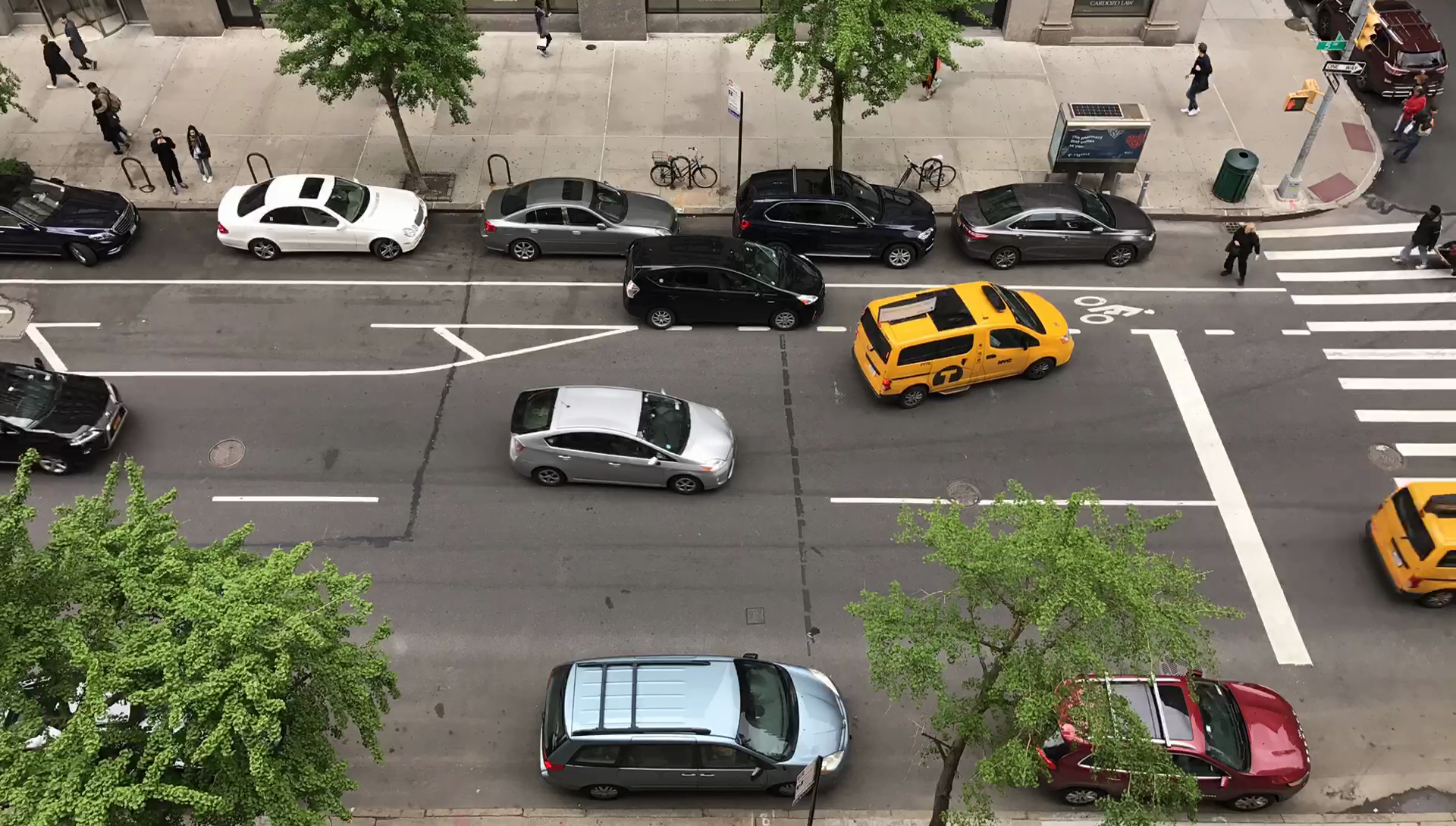
Figure 4: An example image from the collected 5th Avenue dataset of urban videos. These videos include much of the complexity of the real world, including textures, lighting, and uncertain dynamics, while remaining simple enough to model for several frames with a neural network.