CodeX: Bit-Flexible Encoding for Streaming-based FPGA Acceleration of DNNs

Abstract

This paper proposes CodeX, an end-to-end framework that facilitates encoding, bitwidth customization, fine-tuning, and implementation of neural networks on FPGA platforms. CodeX incorporates nonlinear encoding to the computation flow of neural networks to save memory. The encoded features demand significantly lower storage compared to the raw full-precision activation values; therefore, the execution flow of CodeX hardware engine is completely performed within the FPGA using on-chip streaming buffers with no access to the off-chip DRAM. We further propose a fully-automated algorithm inspired by reinforcement learning which determines the customized encoding bitwidth across network layers. CodeX full-stack framework comprises of a compiler which takes a high-level Python description of an arbitrary neural network architecture. The compiler then instantiates the corresponding elements from CodeX Hardware library for FPGA implementation. Proof-of-concept evaluations on MNIST, SVHN, and CIFAR-10 datasets demonstrate an average of $\mathbf{4.65\times}$ throughput improvement compared to stand-alone weight encoding. We further compare CodeX with six existing full-precision DNN accelerators on ImageNet, showing an average of $\mathbf{3.6\times}$ and $\mathbf{2.54\times}$ improvement in throughput and performance-per-watt, respectively.

I Introduction

Deep Neural Networks (DNNs) are being widely developed for various machine learning applications, many of which are required to run on embedded devices. In the realm of embedded DNNs, just-in-time execution under severe power limitations is hard to satisfy [1, 2, 3]. Contemporary research has focused on FPGA-based acceleration of DNNs [4, 5, 6, 7, 8, 9, 10, 11, 12]. However, FPGAs are inherently limited in terms of on-chip memory capacity. Thus, the high-storage requirement of DNN models hinders an efficient and low power execution on FPGAs.

To reduce the computational complexity and memory requirement of DNNs, several pre-processing algorithms have been proposed. The existing methods generally convert conventional DNNs into compact representations that are better suited for execution on embedded devices. Examples of such compacting methods include quantization [13], binarization [7, 10], tensor decomposition [14, 15, 16], parameter pruning [17, 18], and compression with nonlinear encoding [19, 9]. Higher compression rate might not always translate to the hardware performance optimization as the platform constraints could interfere with the intended compaction methodology [20].

This paper specifically focuses on nonlinear encoding and provides solutions to tackle the challenges associated with optimizing physical performance. Encoding network parameters is rather beneficial as it reduces memory footprint, i.e., the main source of delay and power consumption in FPGA accelerators. To devise a practical solution for implementing encoded DNNs, we simultaneously identify and address four critical issues.

First, DNN memory footprint is imposed by either weights or feature-maps. Figure 1 shows the relative memory requirements in several popular DNN models. As can be seen, the memory footprint of activations is notable; however, contemporary research mainly targets the (static) DNN weights for nonlinear quantization [9, 19, 21]. Developing online mechanisms for activation encoding can significantly reduce the memory footprint of DNN models. Second, nonlinear quantization destabilizes DNN training by adding non-differentiable elements to the model. Therefore, novel computation routines must be developed to approximate gradients for DNN fine-tuning. Third, specifying the encoding bitwidth across all DNN layers by handcrafted try-and-error is exhaustive and generally sub-optimal. Hence, automated and intelligent solutions are highly preferable. Finally, designing accelerators that are customized per application/hardware is cumbersome. As such, easy-to-use tools are needed to ensure low, non-recurring engineering cost.

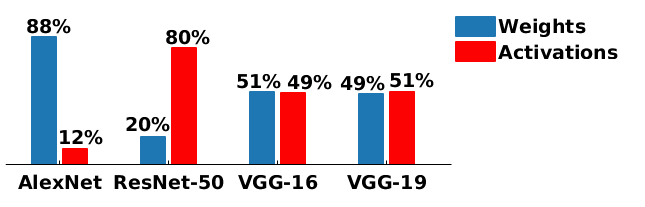
Figure 1: Relative memory footprint of weights and activations for various DNN architectures, evaluated on 10 samples.

To tackle the aforementioned challenges, we introduce CodeX, a unified framework that facilitates encoding, training, bitwidth customization, and automated implementation of encoded DNNs on FPGA platforms. The distinguished contributions of this paper are listed as follows:

• Introducing a novel methodology for (online) encoding of DNN activations. We establish the gradient computation routines required to fine-tune the non-differentiable encoded DNNs, allowing fast restoration of DNN accuracy.

• Introducing an automated algorithm for customizing per-layer encoding bitwidths. Inspired by reinforcement learning, we establish an action-reward-state system to find a bitwidth configuration that minimally affects DNN accuracy and maximally reduces memory footprint.

• Establishing a hardware library for bit-flexible implementation of customized encoded DNN layers. Activation encoding lowers memory footprint and facilitates the use of streaming buffers for inter-layer feature transmission.

• Providing an API for fast and easy hardware implementation of encoded DNNs. Developers describe the DNN as high-level Python code which is then automatically converted to Vivado_HLS (the high-level programming language for Xilinx FPGAs). The API is open-source and can be used by the community.

II Overview and insights

CodeX design flow is composed of an interlinked optimization scheme where algorithmic DNN compaction methods and hardware-level customization for the accelerator are performed in sync. In this section, we describe CodeX insights in high-level and look at the main components of our framework.

II-A Streaming-based On-chip Execution

Traditional DNN accelerators store the weights and activations (features) of layers in the off-chip DRAM since commodity FPGAs are often limited in terms of on-chip memory capacity. Figure 2-top demonstrates the computation flow of DNNs in such settings. Alternatively, the weights and computed activations could be stored and accessed within the FPGA design using streaming buffers as depicted in Figure 2-bottom. The benefits of the latter approach are three-fold. First, it avoids the power-hungry and high-latency access to off-chip DRAM. Second, the computation engines responsible for each DNN layer can be customized to comply with the pertinent layer. Finally, the streaming buffers allow pipelining the computation engines to increase throughput.

Although on-chip execution of DNNs is beneficial in many aspects, the memory requirement of the weights and activations of DNN layers is often beyond the (limited) capacity of commodity FPGAs. To address this issue, CodeX employs nonlinear quantization to reduce the memory footprint such that the weights/activations can be accommodated within FPGA block-RAMs. In the next section, we explain our nonlinear quantization methodology in high level.

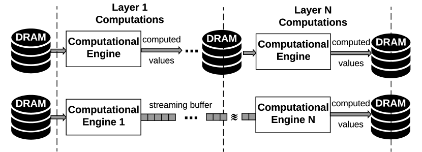
Figure 2: Workflow of traditional vs. streaming-based DNN inference. The top diagram illustrates the conventional approach where all resources are allocated to one computational engine and layer input/outputs are continuously read from and written to the off-chip memory. The bottom diagram presents a streaming-based methodology where communications with off-chip memory are limited to the first and last layer and each layer is allocated a different computational engine.

II-B Memory Compression

In quantization, a finite set of best representatives (a.k.a. bins) are selected and each real-valued number is approximated with the closest bin. Perhaps the most popular quantization is fixed-point approximation. Figure 3-a depicts the bins for an unsigned fixed-point quantization. In this setting, quantization bins are fixed to certain points (e.g., 0, 0.25, …) regardless of data distribution. Alternatively, in nonlinear quantization, the bins are carefully selected to best represent the data. Figure 3-b shows the bins for such nonlinear quantization. In this example, both fixed-point and nonlinear quantizations require the same number of representation bits. However, the approximation error associated with the nonlinear scheme is drastically lower.

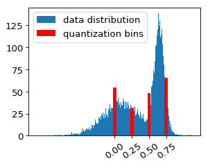
(a) Fixed-point

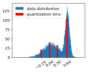
(b) Nonlinear

Figure 3: Illustration of fixed-point and nonlinear quantization. In this example, there are 4 quantization bins and the approximations are represented with $\mathbf{Log_{2}(4)=2}$ bits.

II-C Global Flow

Figure 4 presents the global flow of CodeX framework consisting of an offline processing module, a compiler, and a hardware implementation library.

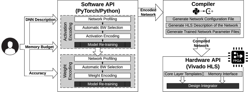
Figure 4: Global flow of CodeX framework. The user provides a high-level Python description of a pre-trained DNN to the pre-processing module, which is responsible for weight/activation encoding, layer-specific bitwidth configuration, and model fine-tuning. The compiler converts the Python code into a hardware description. The hardware API provides a customized library for DNN synthesis and FPGA bitfile generation.

Software API. This module analyzes a given DNN (described in Python code) and applies nonlinear quantization to the layer weights/activations. CodeX encoding scheme reduces memory footprint at the cost of a small reduction in classification accuracy. We devise an automated algorithm to determine the per-layer number of quantization bins for the weights/activations such that the memory footprint is maximally reduced and/or the accuracy is minimally affected. The software API also fine-tunes the quantized DNN to compensate for loss of accuracy.

Hardware API. The DNN hardware is described using Vivado_HLS, which is a standard high-level-synthesis tool that enables faster development as well as portability. CodeX provides a library of template functions that can realize various DNN functionalities. An arbitrary network architecture can be described by instantiating the corresponding templates. Each function has a set of configurable primitives such as the number of input/output neurons of the layer, the weights/activation bitwidths, and the parallelism factors for the layer execution. We will elaborate more on the hardware in Section III-D.

Compiler. To ensure ease-of-use and design automation, CodeX is accompanied by a compiler that converts the high-level Python code for the DNN into a hardware description. CodeX compiler produces a configuration file with the customized per-layer quantization bitwidths. The hardware description together with the configuration file enable instantiation of core layer modules. In addition, the compiler converts the encoded DNN parameters into a format ready for loading to the FPGA on-chip memory upon execution.

III CodeX Software Stack

In this section we elaborate on the concepts utilized for nonlinear encoding of DNN parameters/activations. Section III-A explains CodeX weight/activation encoding method. Our customized gradient computations for training the encoded networks are formulated in Section III-B. Finally, the automated bitwidth selection routine is explained in Section III-C.

III-A Encoding Scheme

Our encoding scheme aims to estimate the parameters of a DNN layer with a subset of representatives referred to as the codebook. In the rest of this section, we delineate CodeX encoding method for DNN weights/activations.

III-A1 Weight Encoding

Let us denote the weight parameters in a certain DNN layer as $W$. In order to encode $W$, we first find an approximation $\widetilde{W}\approx W$ such that the elements of $\widetilde{W}$ are restricted to a finite set of real-values, $\vec{c}=\{c[1],\dots,c[K]\}$, i.e., the codebook. Figure 5 illustrates this approximation for a $4\times 4$ matrix $W$ using a codebook of $K=2$ elements. We denote the encoded $\widetilde{W}$ as $W_{enc}$ where the elements are the index of the corresponding codebook value.

To approximate $\widetilde{W}$ with a codebook of size $K$, authors of [19] suggest using the well-known K-means clustering algorithm [22]. While K-means can effectively solve the aforementioned problem for a fixed codebook size, specifying the codebook sizes in different layers of a neural network is a challenge yet to be solved. Specifically, different layers require different codebook sizes to capture the statistical properties of the pertinent parameters. To tackle this challenge, CodeX proposes an automated bitwidth selection algorithm as explained in Section III-C. Note that weight encoding is performed only once in an offline pre-processing step. The per-layer per-layer encoded weights and codebooks are then stored in binary files to be loaded in the FPGA memory.

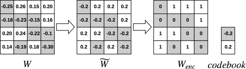
Figure 5: Illustration of CodeX weight encoding. left: original matrix $W$, middle: approximated matrix $\widetilde{W}$, right: encoded matrix $W_{enc}$ along with the codebook vector $c$.

III-A2 Activation Encoding

The encoding of activations is performed in two phases: (i) offline phase performed in CodeX software API, where the layer codebooks are generated using the K-means algorithm. (ii) Online phase where each computed feature is encoded by the closest codebook value.

Offline K-means. Algorithm 1 summarizes the process for computing DNN activation codebooks. First, a subsampled data set, $\vec{x}_{1},\vec{x}_{2},\dots,\vec{x}_{N}$, is used to generate the layer feature-maps, which we denote by $\vec{y}^{\ l}$. Next, $\vec{y}^{\ l}$ is flattened into an array, $\vec{a}^{\ l}$. Since layers with ReLU nonlinearity produce many $0$-valued outputs, we only perform K-means on the non-zero elements of $\vec{a}^{\ l}$ which significantly reduces the runtime of the (offline) K-means clustering. The ($K^{l}-1$) cluster centers along with the appended $0$ value form the $l^{th}$ layer’s codebook.

Online Encoding. The online encoding is performed during FPGA execution. The value of a feature $y$ is compared with the elements of the corresponding layer’s codebook $\vec{c}_{act}^{\ l}$ to compute the encoding as $y_{enc}=argmin(|y-\vec{c}_{act}^{\ l}|)$.

III-B Training of Encoded Networks

Encoding weights/parameters often results in a drop of accuracy. To compensate for such accuracy loss, the codebook entries are fine-tuned after encoding by means of a customized back-propagation scheme. In this section, we explain the details for fine-tuning encoded neural networks via Stochastic Gradient Descent (SGD) [23]. For weights, the averaged gradient method [21, 19] is applied. For activations, we develop new gradient computation methods as follows.

Feature encoding can be viewed as a nonlinear transform which is made up of multiple step functions as depicted in Figure 6. Given the gradient of the loss function with respect to the encoded values, $\nabla_{y^{*}}=\frac{\partial\mathcal{L}}{\partial y^{*}}$, we aim to compute the partial derivatives with respect to the non-encoded values ($\nabla_{y}=\frac{\partial\mathcal{L}}{\partial y}$) and the derivatives with respect to the codebook ($\vec{\nabla}_{c}=\frac{\partial\mathcal{L}}{\partial c}$).

Computing $\mathbf{\nabla_{y}}$. Given the partial derivative $\nabla_{y^{*}}$, the gradient $\nabla_{y}$ can be obtained by applying the chain rule:

This formulation, however, is not stable due to the non-differentiability of the nonlinear function $f(\cdot)$. To address this issue, we propose to approximate the derivative of $f(\cdot)$ as:

where $c[1]$ and $c[K]$ are the smallest and largest codebook values, respectively. During forward propagation, $y^{*}$ is computed as shown in Figure 6-a, whereas the backward propagation assumes the smooth function in Figure 6-b.

Computing $\mathbf{\nabla_{c}}$. Given a scalar gradient element $\nabla_{y^{*}}$, the gradient with respect to $c[k]$ is computed as:

with $I(a,b)=1$ if $a=b$ and zero otherwise (identity operator). Given a vector of features $\vec{y}^{*}$ and the corresponding vector of gradients $\vec{\nabla}_{{y}^{*}}$, the partial derivative is:

Once we compute these partial derivatives, standard back-propagation algorithms can be used to fine-tune DNN parameters. We incorporate the gradient computation routines into CodeX software stack to support fine-tuning for encoded DNNs. As we show in our evaluations, CodeX fine-tuning phase has negligible runtime overhead compared to the original training.

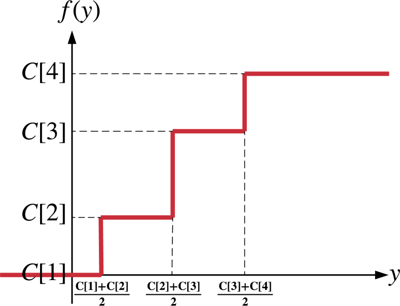
(a)

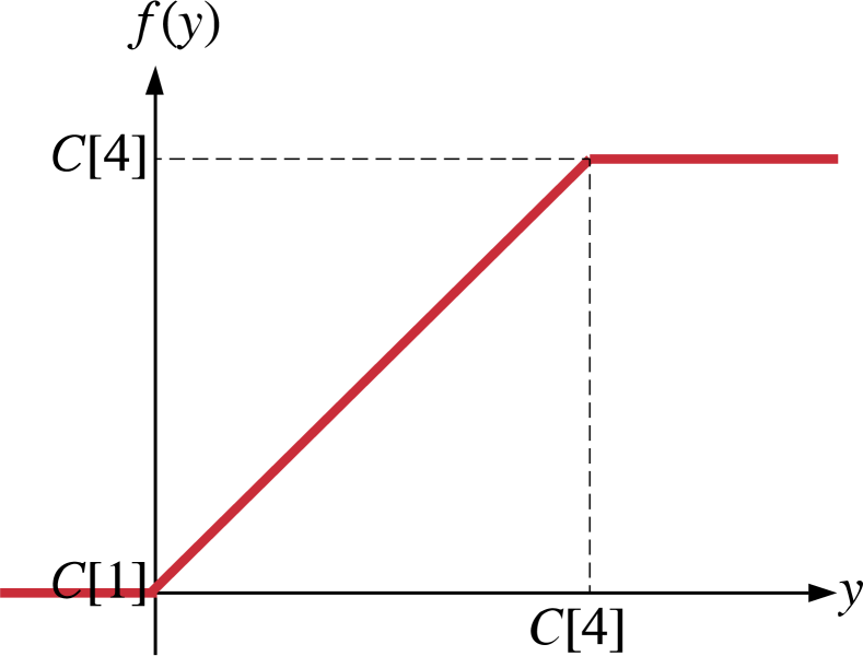
(b)

Figure 6: Example encoding nonlinearity with a codebook of ${K=4}$ elements. (a) Nonlinear function applied in the forward propagation. (b) Smooth approximation of encoding used in backward propagation for gradient computation.

III-C Automated Bitwidth Customization

To alleviate design engineering cost, we propose a bitwidth customization algorithm that automatically determines the encoding bitwidth across all DNN layers. CodeX configures the per-layer numerical precision by changing the codebook size $K$, which translates to the encoding bitwidth $\mathit{ceil(Log_{2}[K])}$; a larger codebook leads to a more accurate approximation which comes at the cost of a higher memory footprint.

CodeX performs a diminishing search over possible bitwidth configurations to capture the trade-off between model accuracy and memory footprint. Algorithm 2 depicts the pseudo-code for our proposed method. Each step of the algorithm starts with an initial configuration of bitwidths, $\mathit{config_{i}}=\{b_{1},\dots,b_{L}\}$ where $b_{l}$ is the $l$-th layer bitwidth and $i$ is the iteration number. Possible next configurations are evaluated by sweeping the bitwidth of $l$-th layer from 1 to $b_{l}-1$ while all other bitwidths are fixed. For a new configuration that sets the $l$-th layer’s bitwidth to $b$, we compute memory reduction $\Delta M(l,b)$ and accuracy drop $\Delta A(l,b)$. Among all candidate configurations, we select the one that maximizes the reward function $\frac{\Delta M(l,b)}{\Delta A(l,b)}$.

The selected candidate is then used as the starting configuration of layer encoding bitwidths in the next iteration. The output of Algorithm 2 is a set of bitwidth configurations, each generated in a certain iteration, that capture the tradeoff between accuracy and the memory footprint. We emphasize that the bitwidth configuration algorithm does not perform any re-training of the DNN in between the iterations. In addition, the inner loop performs accuracy evaluation on a very small subset of validation data (line 8 of Algorithm 2). Therefore, the runtime of CodeX customization is drastically smaller than the original DNN training as we show in the evaluation section.

III-D CodeX Hardware Stack

CodeX is equipped with a hardware library described in high-level synthesis C++ programming language. This library consists of the essential building blocks to implement DNN layers (e.g, convolution, max-pooling, etc.) on FPGA. Each layer-type is implemented as a template function with certain computing engines that are customized to the specifications of the pertinent layer such as the input/output dimensions. By means of this tailoring, CodeX fully exploits the benefits of FPGA reconfigurability and delivers a bit-flexible design.

CodeX adopts a streaming-based architecture which facilitates pipelining and overlays the computational overheads of subsequent DNN layers to increase the overall throughput and minimize latency. Figure 7 presents such pipelined execution for a DNN with $3$ layers. To ensure portability and efficiency, we chose the FINN [10] framework from Xilinx as the base of our hardware accelerator. FINN library was originally intended for execution of Binary Neural Networks (BNNs). We modified the original library to support operations on encoded parameters/weights and fixed-point MAC operations instead of the $\mathit{XnorPopCount}$ operations required in BNNs [10].

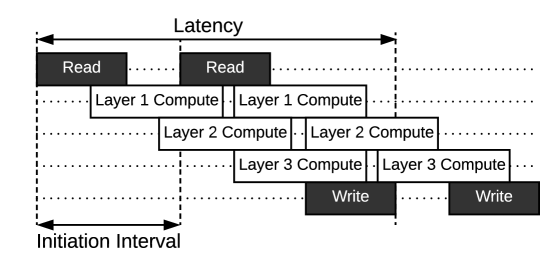
Figure 7: Pipeline execution of layer computations in a streaming-based architecture increases the overall throughput.

Our accelerator is specifically designed to accommodate low-bitwidth encoded networks while supporting full-precision computations. Figure 8 depicts the flow diagram of CodeX accelerator for implementing an encoded DNN on FPGA. The Sliding Window Unit (SWU) reorders the convolution layer input feature-maps to generate appropriate streaming buffers for the Matrix-Vector-Activation Unit (MVAU). The MVAU is the core computational module of CONV and FC layers which performs the matrix-vector multiplication, activation, and batch normalization. The Max-Pooling Unit (MPU) performs max-pooling over the feature-maps. In the following, we discuss the core modules CodeX Hardware API.

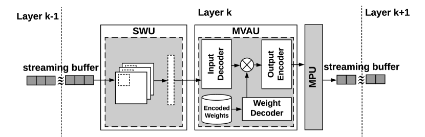
Figure 8: Schematic of CodeX accelerator for encoded DNN inference. SWU reorders the input buffer, MVAU performs the core layer computations, and MPU implements max-pooling.

III-D1 Matrix-Vector-Activation Unit (MVAU)

The MVAU in CodeX hardware library is instantiated in both the convolution (CONV) and fully-connected (FC) layers to generate output features using the corresponding layer’s specifications. Figure 9 illustrates the MVAU computational flow. This module performs $3$ fundamental tasks required in state-of-the-art DNNs, namely matrix-vector multiplication, batch normalization, and applying a non-linear activation. Internally, the MVAU is composed of an array of Processing Engines (PEs) each of which accepts SIMD lanes of input in parallel. In addition, CodeX MVAU has customized encoding/decoding cores for output/input and layer weights.

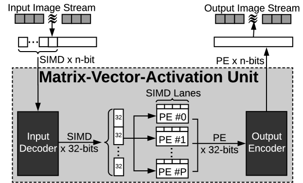
Figure 9: Computational flow of CodeX MVAU. This unit performs matrix-vector multiplication, batch normalization, and a non-linear activation. The MVAU is equipped with an input decoder, an output encoder, and a weight decoder to comply with CodeX encoded networks.

Matrix-Vector Multiplication. The main operations performed in linear DNN layers can be represented as a series of matrix-vector multiplications. The matrix-vector multiplication core in CodeX MVAU offers two levels of parallelism to facilitate throughput control across DNN layers. Firstly, layer output generation is distributed among several PEs working in parallel with each PE responsible for generating the output of multiple feature-map channels (neurons) in a CONV (FC) layer. Furthermore, each PE performs a number of Multiply-Accumulate (MAC) operations in parallel on SIMD inputs. MAC operations are performed in fixed-point on decoded input/weight values, implemented using FPGA DSP slices.

Decoder Modules. Each layer in the encoded DNN contains two decoding codebooks corresponding to the inputs and weights. All codebook values are stored in fixed-point (e.g, 32 bits) and incur a negligible memory footprint. The decoder modules use the encoded values to address a small memory block storing the codebooks. To achieve maximum efficiency, the input decoder is designed such that the values are processed in groups of SIMD elements. To facilitate parallelism, each PE owns a copy of the corresponding weight codebook. Upon execution of the multiply-accumulate operations, the replicated codebooks can be accessed in parallel to decode the weights.

Encoder Module. The combination of ReLU activation function and output encoding is realized by the encoder module. This unit performs a nearest-neighbor search by comparing a fixed-point input value against the encoding codebook and transferring the index of the closest element through the output streaming buffer. Setting the first codebook value to $0$ ensures that the ReLU functionality is inherently applied.

Batch Normalization. For each neuron $x$ in the layer feature-map, batch normalization is equivalent to $\tilde{x}=\alpha x+\beta$ where $\alpha$ is the scaling factor and $\beta$ is the bias value. These values are extracted by CodeX compiler from the trained encoded DNN. In order to implement the batch normalization, each PE in the MVAU performs a single multiplication (by value $\alpha$) and a single addition (with value $\beta$).

III-D2 Sliding Window Unit (SWU)

The convolutional layers of a DNN compute the dot product between a window of the layer input and the CONV weight kernel. The window is slid over the input image to produce individual elements of the output feature-map. The SWU in CodeX hardware simulates the sliding window operation by reordering the values in the layer input image buffer. The input image values are then grouped in chunks of SIMD words to be sent to the MVAU sequentially for processing.

III-D3 Max-pooling Unit (MPU)

CodeX software stack outputs a sorted list of codebook values for the encoded layer activations where the clusters centers with higher values are mapped to larger cluster indices. This sorting is particularly useful since comparison over encoded values becomes equivalent to comparison over the original fixed-point values; therefore, CodeX performs the max-pooling operation on low-bitwidth encoded values rather than the full-precision cluster centers. This approach provides two benefits: 1) the memory overhead of the buffers in the MPU is considerably reduced. 2) The logic cost of comparison between low-bitwidth encoded values is significantly smaller than the full-precision counterpart.

IV Experiments

To evaluate CodeX effectiveness, we perform proof-of-concept experiments on four different classification benchmarks, namely, MNIST, SVHN, CIFAR-10, and ImageNet. We implement CodeX software API in Pytorch library. The hardware API is realized in Vivado_HLS design suite. All hardware resource utilizations are gathered after performing place-and-route via Vivado Design Suite 2017.2. Throughput values are reported from Vivado_HLS 2017.2.

IV-A CodeX Automated Bitwidth Selection

We illustrate our bitwidth selection algorithm (Section III-C) using the AlexNet architecture [24] trained on ImageNet dataset which contains $50000$ test samples. To perform customization, we split these images into $49000$ test and $1000$ validation samples. The validation data is used for bitwidth selection whereas the test data is utilized to report classification accuracy.

Configuring Activation Bitwidths. The first step of CodeX bitwidth customization is to encode the activations while the weights are kept at full-precision. Figure 10-a demonstrates the iterative process of bitwidth selection for network activations. Here, each colored square at location $(l,i)$ represents the encoding bitwidth for the $l$-th layer’s activation at step $i$ of the algorithm where $l$ and $i$ span the vertical and horizontal axes, respectively. Initially, the activations are encoded with $b_{enc}=5$ bits. As the algorithm proceeds, both the total memory footprint and DNN accuracy are decreased. The algorithm terminates when the accuracy drops below a threshold of $10\%$. We next select one of the configurations (corresponding to the column with bold border) in Figure 10-a and perform fine-tuning to recover accuracy. We then proceed to the weight encoding step.

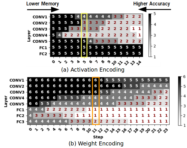
Figure 10: Per-layer bitwidth configuration at each step of CodeX bitwidth selection algorithm, shown for AlexNet.

Configuring Weight Bitwidths. Initially, the CONV and FC weights are encoded with $b_{enc}=6$ and $b_{enc}=4$ bits, respectively. During this customization step, the activation bitwidths remain unchanged and only the weight bitwidths are configured. The corresponding bitwidths of network weights in different iterations of the algorithm are depicted in Figure 10-b and the selected weight configuration is highlighted by bold borders. Note that CodeX enjoys the flexibility of selecting various pairs of activation-weight configurations depending on accuracy and memory constraints.

Discussion on Selected Bitwidths. CodeX aims at capturing the memory/accuracy tradeoff spanned by the bitwidth configurations. Consider the selected configuration of Figure 10-b as an example. CONV layers have more effect on model accuracy, requiring a high encoding bitwidth. In addition, the contribution of FC layers to the overall weight memory footprint is much higher than that of CONV layers. As a result, FC layers are encoded with fewer bits compared to CONV layers.

Comparison with Prior Art. To compare CodeX with existing low-bit neural networks, we train several widely popular architectures summarized in Table I. We then select a set of customized cross-layer encoding configurations generated by CodeX bitwidth selection mechanism. Each of our examined architectures and their corresponding bitwidths are chosen specifically to match the accuracy and/or memory footprint of prior art. As such, for some architectures, e.g, VGG7, multiple configurations are evaluated that merely differ in number of weight bits. Figure 11 shows the selected per-layer bitwidths for the weights and activations of each DNN configuration.

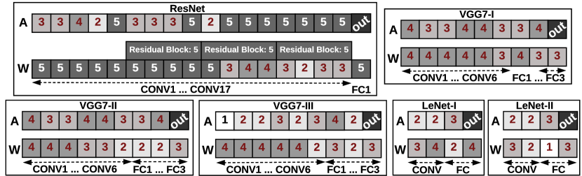
Figure 11: Per-layer encoding bitwidths for evaluated DNNs.

TABLE I: Summary of evaluated network architectures in terms of the number of convolutions (CONV), max-pooling (MP), global average pooling (AP), and fully connected (FC) layers.

Dataset	Network	Description
MNIST	LeNet	2 CONV, 2 MP, 2 FC
SVHN & CIFAR-10	VGG7	6 CONV, 2 MP, 3 FC
ImageNet	AlexNet	5 CONV, 3 MP, 3 FC
	ResNet	17 CONV, 1 MP, 1 AP, 1 FC

Table II compares the selected configurations with prior art in terms of memory, accuracy, and fine-tuning time. It is worth mentioning that, unlike existing low-bit DNNs which train the whole network from scratch, CodeX takes a post-processing approach that is readily applied to pre-trained neural networks. The importance of this property is two-fold: (i) CodeX eliminates the drastic cost of training from scratch per bitwidth configuration. Using our fine-tuning method explained in Section III-B, the model accuracy is retrieved after few epochs, e.g., as low as 0.25 epochs for ImageNet. (ii) CodeX customization can be applied to pre-trained models that are publicly available online.

TABLE II: Comparison of CodeX with state-of-the-art low-bit DNNs. The per-layer bitwidths for AlexNet are shown in Figure 10. The bitwidths for LeNet-X, VGG7-X, and ResNet models are same as those in Figure 11.

	Baselines	Arch	Test Acc	Mem	Epochs	Bitwidth
						Weight	Act
MNIST	QNN [13]	MLP	99.04	$193\times$	1000	1	1
	ReBNet3 [7]	MLP	98.25	$1.76\times$	200	1	2
	CodeX	LeNet-I	99.02	$1.84\times$	$10\times 2^{*}$	flexible
	CodeX	LeNet-II	98.31	$1$	$10\times 2$	flexible
CIFAR-10	QNN [13]	VGG7	89.85	$5.4\times$	500	1	1
	ReBNet3 [7]	VGG7	86.98	$1.65\times$	200	1	3
	CodeX	VGG7-I	88.14	$1.32\times$	$10\times 2$	flexible
	CodeX	VGG7-II	87.01	$1$	$10\times 2$	flexible
SVHN	ReBNet3 [7]	VGG7	97.00	$1.62\times$	50	1	3
	QNN [13]	VGG7	97.2	$2.15\times$	200	1	1
	CodeX	VGG7-III	97.15	$1$	$10\times 2$	flexible
ImageNet	HWGQ [25]	AlexNet	52.70	$1.17\times$	68	1	2
	QNN [13]		51.03	$1.17\times$	-	1	2
	DoReFaNet [26]		49.80	$1.17\times$	45	1	2
	WRPN [27]‡		48.30	$4.61\times$	-	1	1
	XNORNet [28]		44.20	$1.15\times$	18	1	1
	ReBNet3 [7]		41.43	$1.17\times$	100	1	3
	CodeX		53.21	$1$	$0.25\times 2$	flexible
	ABC-Net [29]	ResNet18	65.00	$1.57\times$	-	5	5
	ABC-Net [29]		62.50	$1.05\times$	-	3	5
	CodeX		65.40	$1$	$0.25\times 2$	flexible

^∗fine-tuning for 10 epochs post-activation and 10 epochs post-weight encoding.
^‡ This baseline has $2\times$ more neurons per layer.

Overhead of Customization and Re-training: Table III report CodeX customization overhead for our most complex benchmark, i.e., ResNet. The customization phase incurs roughly $8.5\%$ of the training time. Note that the bitwidth customization phase is performed offline, prior to design synthesis and hardware evaluation.

TABLE III: Breakdown of customization overhead for ResNet-18 network, namely, activation encoding (AE), fine-tuning (FT), and weight encoding (WE). The number of training epochs is extracted from the original ResNet paper [30]. The timing is reported for a machine running a single Nvidia Titan Xp GPU.

Customization	AE	FT	WE	FT	Total
	114 mins	4 mins	31 mins	4 mins	153 mins
Training	-	-	-	-	1800 mins

IV-B CodeX Hardware Implementation

In this section, we evaluate CodeX hardware accelerator. We implement one architecture per dataset from Figures 10 and 11, namely, LeNet-I for MNIST, VGG7-I for CIFAR10, VGG7-III for SVHN, and AlexNet for ImageNet. Table IV summarizes the evaluation platforms for each DNN architecture.

TABLE IV: Platform details in terms of block ram (BRAM), DSP, flip-flop (FF), and look-up table (LUT) resources.

Application	Platform	BRAM	DSP	FF	LUT
ImageNet	Virtex VCU108	3456	768	1075200	537600
CIFAR-10 & SVHN	Zynq ZC702	280	220	106400	53200
MNIST	Spartan XC7S50	120	150	65200	32600

Importance of Activation Encoding. We start the analysis by studying the advantages of activation encoding, from the hardware perspective, versus solely encoding the weights as proposed in [19]. Note that [19] also applies pruning and Huffman encoding which are the main contributors to the compression rate. Since these methods are orthogonal to our approach, we do not utilize them in CodeX to focus on the analysis of encoding itself. We compare two versions of encoded DNNs: one with encoded weights and fixed-point activations as proposed in [19], and another with both weights and activations encoded as suggested in CodeX. For each dataset, we separately optimize the per-layer parallelism factors SIMD and PE for both encoded and fixed-point DNNs to obtain maximum throughput while complying with the resource constraints. Table V summarizes the resource utilization and throughput for each of the designs.

Overall, realization of CodeX methodology, i.e., $\mathit{DNN_{enc}}$, achieves higher throughput while requiring lower number of resources compared to a weight-only encoding approach [19]. The benefits become more prominent for architectures with higher complexity since the memory implication of activations contributes more in complex networks. As seen for MNIST, CIFAR-10, and SVHN benchmarks, CodeX activation encoding improves the throughput by $1.1\times$, $6.2\times$, and $6.66\times$, respectively. The effect of activation encoding is most significant for the ImageNet benchmark; the memory of the model with fixed-point activations is larger than the capacity of the on-chip streaming buffers, rendering the design infeasible within platform constraints. For this dataset, we compare $\mathit{DNN_{enc}}$ with existing fixed-point accelerators in the following.

TABLE V: Summary of hardware resource utilization and performance. $\mathit{DNN_{enc}}$ stands for the model with encoded weights and activations whereas $\mathit{DNN_{fix}}$ denotes the network with encoded weights and (8-bit) Fixed-point activations.

		Resource Utilization				Latency (ms)
		BRAM	DSP∗	FF	LUT
MNIST	$\mathit{DNN_{enc}}$	33	53	15223	9992	0.39
	$\mathit{DNN_{fix}}$	93	53	25884	12048	0.43
	$\mathit{Ratio}$	$2.82\times$	$1\times$	$1.7\times$	$1.2\times$	1.1$\times$
CIFAR-10	$\mathit{DNN_{enc}}$	197	111	53953	31632	3.58
	$\mathit{DNN_{fix}}$	181	35	68255	28433	22.21
	$\mathit{Ratio}$	$0.92\times$	$0.32\times$	$1.26\times$	$0.9\times$	6.2$\times$
SVHN	$\mathit{DNN_{enc}}$	146	111	42748	28393	3.39
	$\mathit{DNN_{fix}}$	143	35	67944	27934	22.59
	$\mathit{Ratio}$	$0.98\times$	$0.32\times$	$1.59\times$	$0.98\times$	6.66$\times$
ImageNet	$\mathit{DNN_{enc}}$	3336	308	159663	82791	25.05
	$\mathit{DNN_{fix}}$	Exceeds Platform Constraints

${}^{*}25\times 18$ DSB array.

Comparison with Fixed-point Accelerators. We perform a comprehensive comparison between CodeX and prior work in Table VI. Specifically, we consider AlexNet with customized encoding as in Figure 10, which corresponds to hardware results of Table V. The reported results include performance, either in terms of throughput (frames per second) or latency. Since the existing frameworks utilize various hardware platforms, it is crucial to take into account the instantiated computational capacity and power consumption. Therefore, we compare the frameworks by means of performance-per-resource and performance-per-Watt. CodeX achieves higher normalized performance compared to prior art. This is a direct result of using on-chip memory instead of the off-chip DRAM for feature transfer among DNN layers. The streaming buffers of our design allow CodeX to better utilize the arithmetic units by overlapping the execution of DNN layers, achieving a higher performance-per-resource. The power advantage of CodeX over existing accelerators is also rooted in the elimination of power-hungry DRAM access.

TABLE VI: Comparison of Alexnet implementation between CodeX and existing fixed-point (FXD) and floating-point (FLT) DNN accelerators. To account for platform variations, we compare the throughput (frames-per-second) and $\frac{\textrm{1}}{\textrm{Latency}}$ metrics normalized by computation capacity (CAP). We also compare performance-per-Watt to reflect power efficiency.

	Criterion	[31]	[6]	[32]	[33]	[8]	[34]	CodeX
	Precision	FLT	FXD	FXD	FXD	FXD	FXD	Flexible
	Acc(%)	-	55.41	52.4	56.5	-	54.27	53.2
	FPGA	690T∗	GSD8†	690T∗	690T∗	AX115‡	ZU9§	VCU108∗
	Freq(MHz)	100	120	150	100	200	300	152
	DSP∗∗	3177	1504	14400	2872	2688	442	308
Throughput	/CAP	0.55$\times$	1	0.88$\times$	2.33$\times$	1.42$\times$	0.49$\times$	3.03$\times$
	/Watt	3.14$\times$	1	1.82$\times$	5.00$\times$	1.36$\times$	-	4.54$\times$
$\frac{\textrm{1}}{\textrm{Latency}}$	/CAP	-	1	0.05$\times$	0.15$\times$	-	-	3.03$\times$
	/Watt	-	1	0.10$\times$	0.32$\times$	-	-	4.54$\times$

^∗Virtex     ^†Stratix-V    ^‡Arria10    ^§Zynq
^∗∗DSP array size is $25\times 18$ for Xilinx and $18\times 18$ for Altera/Intel FPGAs.

Execution Overhead of Encoding/Decoding. We study the runtime implication of online activation encoding by measuring the number of clock cycles required for different stages of CodeX MVAU engine. Figure 12 demonstrates the runtime break-down for each of the evaluated architectures. For a conventional non-encoded network, the MVAU would only perform Vector-Dot-Product (VDP) operations. As can be seen, for CodeX encoded models, the majority of clock cycles in MVAU execution belong to VDP computation while the encoding/decoding overhead is negligible.

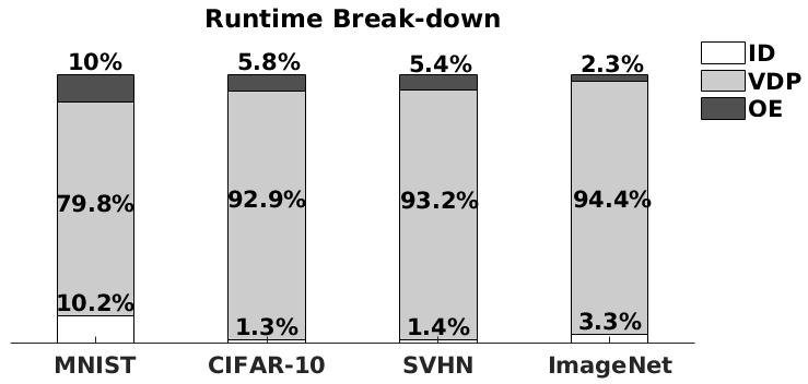
Figure 12: Runtime breakdown of Input Decoding (ID), Vector-Dot-Product (VDP), and Output Encoding (OE) across layers.

V Related Work

As neural networks are memory-intensive, devising methods to decrease the memory footprint can significantly enhance accelerator performance in terms of throughput and power consumption. An attractive solution for memory reduction is training few-bit DNNs. Several methods for training DNNs with few bits have been proposed in [26, 27, 25, 28, 13, 29]. These papers focus on the establishment of the theoretical foundation for low-bit DNN inference. Nevertheless, the inference accuracy of these DNNs is often lower than the original full-precision model. Higher accuracy can be achieved using DNN models that perform computations in the fixed-point regime.

Nonlinear encoding allows for utilization of fixed-point arithmetics accompanied by a low storage requirement. Perhaps the closest method to this paper is a stand-alone weight encoding, with no activation encoding, originally proposed in [19, 21, 9]. Weight encoding significantly reduces the memory footprint of model parameters but the activation units (especially in convolution layers) still require a large capacity of memory. To address this challenge, we extend the encoding to the activations of neural networks and introduce training routines for the corresponding encoded activations. In addition, prior work utilizes hand-crafted or rule-based heuristics to determine the encoding bitwidth. Such manual methods are generally sub-optimal and incur a drastic engineering cost. To address this issue, we propose an automated cross-layer bitwidth selection algorithm that aims to capture the accuracy/memory tradeoff.

In a concurrent track, designing automated and easy-to-use tools for FPGA implementation of DNNs has been the focus of contemporary research [31, 6, 32, 33, 8, 34]. These works aim to maximize the throughput of fixed/floating-point DNN inference by distributing FPGA resources among parallel computational engines. Although accurate, fixed-point DNNs are generally memory intensive, where excessive access to off-chip memory becomes a design bottleneck. To alleviate this problem, authors of [10, 7] propose to perform inference solely using the on-chip memory and utilizing streaming buffers to realize inter-layer data transfers. These frameworks facilitate the design process of DNNs by providing configurable template functions in high-level synthesis language. However,  [10, 7] are only compatible with binary DNNs as their core computational engines do not support fixed-point arithmetics. By incorporating activation encoding into DNN computational flow, CodeX hardware simultaneously enjoys the performance benefits of on-chip streaming buffers and the high accuracy of fixed-point arithmetics. CodeX hardware stack supports flexible bitwidths, allowing the implementation of customized encoded DNNs.

VI Conclusion

This paper proposes a novel nonlinear quantization scheme to reduce the memory footprint of intermediate activations in convolutional neural networks computation flow. The encoding compresses the activations and allows on-chip execution of the underlying FPGA accelerator without communicating the computed features with the off-chip DRAM. To ensure non-recurring engineering cost, an automated algorithm is proposed to configure the encoding bitwidth across all layers of an arbitrary neural network. The open-source API of CodeX enables developers to convert high-level Pytorch description of the neural network into hardware description without getting involved with the details of the design. We hope the provided API can advance research on reconfigurable DNN inference.

References

- [1] D. Li, X. Wang, and D. Kong, “Deeprebirth: Accelerating deep neural network execution on mobile devices,” arXiv preprint arXiv:1708.04728, 2017.
- [2] X. Zhang, X. Zhou, M. Lin, and J. Sun, “Shufflenet: An extremely efficient convolutional neural network for mobile devices,” arXiv preprint arXiv:1707.01083, 2017.
- [3] A. G. Howard, M. Zhu, B. Chen, D. Kalenichenko, W. Wang, T. Weyand, M. Andreetto, and H. Adam, “Mobilenets: Efficient convolutional neural networks for mobile vision applications,” arXiv preprint arXiv:1704.04861, 2017.
- [4] C. Zhang, P. Li, G. Sun, Y. Guan, B. Xiao, and J. Cong, “Optimizing fpga-based accelerator design for deep convolutional neural networks,” in Proceedings of the 2015 ACM/SIGDA International Symposium on Field-Programmable Gate Arrays. ACM, 2015, pp. 161–170.
- [5] K. Ovtcharov, O. Ruwase, J.-Y. Kim, J. Fowers, K. Strauss, and E. S. Chung, “Accelerating deep convolutional neural networks using specialized hardware,” Microsoft Research Whitepaper, vol. 2, no. 11, 2015.
- [6] N. Suda, V. Chandra, G. Dasika, A. Mohanty, Y. Ma, S. Vrudhula, J.-s. Seo, and Y. Cao, “Throughput-optimized opencl-based fpga accelerator for large-scale convolutional neural networks,” in Proceedings of the 2016 ACM/SIGDA International Symposium on Field-Programmable Gate Arrays. ACM, 2016, pp. 16–25.
- [7] M. Ghasemzadeh, M. Samragh, and F. Koushanfar, “Rebnet: Residual binarized neural network,” in 2018 IEEE 26th Annual International Symposium on Field-Programmable Custom Computing Machines (FCCM). IEEE, 2018, pp. 57–64.
- [8] H. Sharma, J. Park, D. Mahajan, E. Amaro, J. K. Kim, C. Shao, A. Mishra, and H. Esmaeilzadeh, “From high-level deep neural models to fpgas,” in The 49th Annual IEEE/ACM International Symposium on Microarchitecture. IEEE Press, 2016, p. 17.
- [9] M. Samragh, M. Ghasemzadeh, and F. Koushanfar, “Customizing neural networks for efficient fpga implementation,” in Field-Programmable Custom Computing Machines (FCCM), 2017 IEEE 25th Annual International Symposium on. IEEE, 2017, pp. 85–92.
- [10] Y. Umuroglu, N. J. Fraser, G. Gambardella, M. Blott, P. Leong, M. Jahre, and K. Vissers, “Finn: A framework for fast, scalable binarized neural network inference,” in Proceedings of the 2017 ACM/SIGDA International Symposium on Field-Programmable Gate Arrays. ACM, 2017, pp. 65–74.
- [11] A. Prost-Boucle, A. Bourge, F. Pétrot, H. Alemdar, N. Caldwell, and V. Leroy, “Scalable high-performance architecture for convolutional ternary neural networks on fpga,” 2017.
- [12] C. Shea, A. Page, and T. Mohsenin, “Scalenet: A scalable low power accelerator for real-time embedded deep neural networks,” in Proceedings of the 2018 on Great Lakes Symposium on VLSI. ACM, 2018, pp. 129–134.
- [13] I. Hubara, M. Courbariaux, D. Soudry, R. El-Yaniv, and Y. Bengio, “Quantized neural networks: Training neural networks with low precision weights and activations,” arXiv preprint arXiv:1609.07061, 2016.
- [14] Y.-D. Kim, E. Park, S. Yoo, T. Choi, L. Yang, and D. Shin, “Compression of deep convolutional neural networks for fast and low power mobile applications,” arXiv preprint arXiv:1511.06530, 2015.
- [15] X. Zhang, J. Zou, X. Ming, K. He, and J. Sun, “Efficient and accurate approximations of nonlinear convolutional networks,” in Proceedings of the IEEE Conference on Computer Vision and Pattern Recognition, 2015, pp. 1984–1992.
- [16] M. Nazemi, A. E. Eshratifar, and M. Pedram, “A hardware-friendly algorithm for scalable training and deployment of dimensionality reduction models on FPGA,” in Proceedings of the 19th IEEE International Symposium on Quality Electronic Design, 2018.
- [17] B. Liu, M. Wang, H. Foroosh, M. Tappen, and M. Pensky, “Sparse convolutional neural networks,” in Proceedings of the IEEE Conference on Computer Vision and Pattern Recognition, 2015, pp. 806–814.
- [18] W. Wen, C. Wu, Y. Wang, Y. Chen, and H. Li, “Learning structured sparsity in deep neural networks,” in Advances in Neural Information Processing Systems, 2016, pp. 2074–2082.
- [19] S. Han, H. Mao, and W. J. Dally, “Deep compression: Compressing deep neural networks with pruning, trained quantization and huffman coding,” arXiv preprint arXiv:1510.00149, 2015.
- [20] T.-J. Yang, A. Howard, B. Chen, X. Zhang, A. Go, V. Sze, and H. Adam, “Netadapt: Platform-aware neural network adaptation for mobile applications,” arXiv preprint arXiv:1804.03230, 2018.
- [21] W. Chen, J. T. Wilson, S. Tyree, K. Q. Weinberger, and Y. Chen, “Compressing neural networks with the hashing trick,” CoRR, abs/1504.04788, 2015.
- [22] S. Lloyd, “Least squares quantization in pcm,” IEEE transactions on information theory, vol. 28, no. 2, pp. 129–137, 1982.
- [23] J. Kiefer, J. Wolfowitz et al., “Stochastic estimation of the maximum of a regression function,” The Annals of Mathematical Statistics, vol. 23, no. 3, pp. 462–466, 1952.
- [24] A. Krizhevsky, I. Sutskever, and G. E. Hinton, “Imagenet classification with deep convolutional neural networks,” in Advances in neural information processing systems, 2012, pp. 1097–1105.
- [25] Z. Cai, X. He, J. Sun, and N. Vasconcelos, “Deep learning with low precision by half-wave gaussian quantization,” arXiv preprint arXiv:1702.00953, 2017.
- [26] S. Zhou, Y. Wu, Z. Ni, X. Zhou, H. Wen, and Y. Zou, “Dorefa-net: Training low bitwidth convolutional neural networks with low bitwidth gradients,” arXiv preprint arXiv:1606.06160, 2016.
- [27] A. Mishra, E. Nurvitadhi, J. J. Cook, and D. Marr, “Wrpn: wide reduced-precision networks,” arXiv preprint arXiv:1709.01134, 2017.
- [28] M. Rastegari, V. Ordonez, J. Redmon, and A. Farhadi, “Xnor-net: Imagenet classification using binary convolutional neural networks,” in European Conference on Computer Vision. Springer, 2016, pp. 525–542.
- [29] X. Lin, C. Zhao, and W. Pan, “Towards accurate binary convolutional neural network,” in Advances in Neural Information Processing Systems, 2017, pp. 345–353.
- [30] K. He, X. Zhang, S. Ren, and J. Sun, “Deep residual learning for image recognition,” in Proceedings of the IEEE conference on computer vision and pattern recognition, 2016, pp. 770–778.
- [31] Y. Shen, M. Ferdman, and P. Milder, “Maximizing cnn accelerator efficiency through resource partitioning,” in Computer Architecture (ISCA), 2017 ACM/IEEE 44th Annual International Symposium on. IEEE, 2017, pp. 535–547.
- [32] C. Zhang, D. Wu, J. Sun, G. Sun, G. Luo, and J. Cong, “Energy-efficient cnn implementation on a deeply pipelined fpga cluster,” in Proceedings of the 2016 International Symposium on Low Power Electronics and Design. ACM, 2016, pp. 326–331.
- [33] Z. Liu, Y. Dou, J. Jiang, J. Xu, S. Li, Y. Zhou, and Y. Xu, “Throughput-optimized fpga accelerator for deep convolutional neural networks,” ACM Transactions on Reconfigurable Technology and Systems (TRETS), vol. 10, no. 3, p. 17, 2017.
- [34] “Chaidnn: Hls based deep neural network accelerator library for xilinx ultrascale+ mpsocs,” https://github.com/Xilinx/CHaiDNN.