Globally Optimal Departure Rates for Several Groups of Drivers

Abstract

The first part of this paper contains a brief introduction to conservation law models of traffic flow on a network of roads. Globally optimal solutions and Nash equilibrium solutions are reviewed, with several groups of drivers sharing different cost functions.

In the second part we consider a globally optimal set of departure rates, for different groups of drivers but on a single road. Necessary conditions are proved, which lead to a practical algorithm for computing the optimal solution.

Keywords: Conservation law, traffic flow, globally optimal solution.

1 Introduction

Macroscopic models of traffic flow, first introduced in [25, 27], have now become a topic of extensive research. On a single road, the evolution of the traffic density can be described by a scalar conservation law. In order to extend the model to a whole network of roads, additional boundary conditions must be inserted, describing traffic flow at each intersection; see [10, 15, 19, 20, 22, 23] or the survey [4]. A major eventual goal of these models is to understand traffic patterns, determined by the behavior of a large number of drivers with different origins and destinations.

In a basic setting, one can consider $N$ groups of drivers, say ${\cal G}_{1},\ldots,{\cal G}_{N}$. Drivers from each group have the same origin and destination, and a cost which depends on their departure and arrival time. For such a model, two kind of solutions are of interest:

• The Nash equilibrium solution, where each driver chooses his own departure time and route to destination, in order to minimize his own cost.

• The global optimization problem, where a central planner seeks to schedule all departures in order to minimize the sum of all costs.

In general, these criteria determine very different traffic patterns. To fix the ideas, let $t\mapsto u_{i}(t)$, $i=1,\ldots,N$, be the departure rate of drivers of the $i$-th group, so that

$$\int_{-\infty}^{t}u_{i}(s)\,ds$$

yields the total number of these drivers who depart before time $t$. We recall that the support of $u_{i}$, denoted by Supp$(u_{i})$, is the closure of set of times $t$ where $u_{i}(t)>0$.

Roughly speaking, the two above solutions can be characterized as follows.

(I) In a Nash equilibrium, all drivers within the same group pay the same cost. Namely, there exists constants $K_{1},\ldots,K_{N}$ such that

• every driver of the $i$-th group, departing at a time $t\in Supp(u_{i})$ bears the cost $K_{i}$.

• if a driver of the $i$-th group were to depart at any time $t\in I\!\!R$ (possibly outside the support of $u_{i}$), he would incur in a cost $\geq K_{i}$.

(II) For a global optima, there exist constants $C_{1},\ldots,C_{n}$ (where $C_{i}$ is the marginal cost for adding one more driver of the $i$-th group) such that

• If one additional driver of the $i$-th group is added at any time $t\in\hbox{Supp}(u_{i})$, then the total cost increases by $C_{i}$.

• If one additional driver of the $i$-th group is added at any time $t\in I\!\!R$ (possibly outside the support of $u_{i}$), then the increase in the total cost is greater or equal to $C_{i}$.

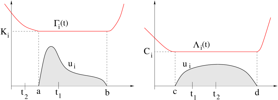
At an intuitive level, these conditions are easy to explain. In Fig. 1, left, the function $\Gamma_{i}(t)$ denotes the cost to an $i$-driver departing at time $t$. If $\Gamma_{i}$ did not attain its global minimum simultaneously at all points $t\in[a,b]=\hbox{Supp}(u_{i})$, then we could find times $t_{1}\in[a,b]$ and $t_{2}\in I\!\!R$ such that $\Gamma_{i}(t_{2})<\Gamma_{i}(t_{1})$. In this case, the driver departing at time $t_{1}$ could lower his own cost choosing to depart at time $t_{2}$ instead. This contradicts the definition of equilibrium.

In Fig. 1, right, the function $\Lambda_{i}(t)$ denotes the marginal cost for inserting one additional driver of the $i$-th family, departing at time $t$. This accounts for the additional cost to the new driver, and also for the increase in the cost to all other drivers who are slowed down by the presence of one more car on the road. If $\Lambda_{i}$ did not attain its global minimum at all points in $[c,d]=\hbox{Supp}(u_{i})$, then we could find times $t_{1}\in[c,d]$ and $t_{2}\in I\!\!R$ such that $\Lambda_{i}(t_{2})<\Lambda_{i}(t_{1})$. In this case we could consider a new traffic pattern, with one less driver departing at time $t_{1}$ and one more departing at time $t_{2}$. This would achieve a smaller total cost, contradicting the assumption of optimality.

Figure 1: Left: the rate of departures $u_{i}$, for drivers of the $i$-th group, in a Nash equilibrium solution. Each of these drivers starts at some time $t\in[a,b]$. To achieve an equilibrium, the cost $\Gamma_{i}(t)$ to any driver departing at time $t$ must be constant inside $[a,b]$ and larger outside. Right: the rate of departures $u_{i}$, in a globally optimal solution. Here $\Lambda_{i}(t)$ denotes the marginal cost for inserting an additional driver of the $i$-th group, departing at time $t$. To achieve global optimality, $\Lambda_{i}$ must be constant on the support of $u_{i}$, and larger outside.

While the criterion (I) for an equilibrium solution is easy to justify, a rigorous proof of the necessary condition (II) for a global optimum faces considerable difficulties. Indeed, to compute the “marginal cost” for adding one more driver, one should differentiate the solution of a conservation law w.r.t. the initial data (or the boundary data). As it is well known, in general one does not have enough regularity to carry out such a differentiation. To cope with this difficulty one can introduce a “shift differential”, describing how the shock locations change, depending on parameters. See [8, 9, 13, 26, 29] for results in this direction.

The first part of this paper contains an introduction to macroscopic models of traffic flow on a network of roads. Section 2 starts by reviewing the classical LWR model for traffic flow on a single road, in terms of a scalar conservation law for the traffic density. We then discuss various boundary conditions, modeling traffic flow at an intersection. Finally, given a cost function depending on the departure and arrival times of each driver, we review the concepts of globally optimal solution and of Nash equilibrium solution.

The second part of paper contains original results. We consider here $N$ groups of drivers traveling along the same road, but with different departure and arrival costs. We seek departure rates $u_{1}(\cdot),\ldots,u_{N}(\cdot)$ which are globally optimal. Namely, they minimize the sum of all costs to all drivers. A set of necessary conditions for optimality is derived, thus extending the result in [5] to the case where several groups of drivers are present. Relying on these conditions, in the last section we introduce an algorithm that numerically computes such globally optimal solutions.

For an introduction to the general theory of conservation laws we refer to [3, 18, 28]. A more comprehensive discussion of various models of traffic flow can be found in [1, 2, 17, 19].

2 Conservation law models for traffic flow

2.1 Traffic flow on a single road.

According to the classical LWR model [25, 27], traffic density on a single road can be described in terms of a scalar conservation law

$$\rho_{t}(t,x)+f(\rho(t,x))_{x}~{}=~{}0.$$ (2.1)

Here $t$ is the time, while $x\in I\!\!R$ is the space variable along the road. Moreover

• $\rho$ is the traffic density, i.e., the number of cars per unit length of the road.

• $v=v(\rho)$ is the velocity of cars, which we assume depends only the traffic density.

• $f=f(\rho)$ is the flux, i.e., the number of cars crossing a point $x$ along the road, per unit time. We have the identity

  $$\hbox{[flux]}~{}=~{}\hbox{[density]$\times$[velocity]}~{}=~{}\rho\cdot v(\rho)$$

As shown in Fig. 2, the velocity should be a decreasing function of the car density. Concerning the flux function, a natural set of assumptions is

$$f\in{\cal C}^{2},\qquad f^{\prime\prime}<0,\qquad f(0)=f(\rho_{jam})=0.$$ (2.2)

Here $\rho_{jam}$ is the maximum density of cars allowed on the $k$-th road. This corresponds to bumper-to-bumper packing, where no car can move.

Smooth solutions of the conservation law (2.1) can be computed by the classical method of characteristics. By the chain rule, one obtains

$$\rho_{t}+f^{\prime}(\rho)\rho_{x}~{}=~{}0.$$ (2.3)

Hence, if $t\mapsto x(t)$ is a curve such that

$$\dot{x}(t)~{}\doteq~{}{d\over dt}x(t)~{}=~{}f^{\prime}(\rho(t,x(t))),$$ (2.4)

then the equation (2.3) yields

$${d\over dt}\rho(t,x(t))~{}=~{}\rho_{t}+\rho_{x}\,\dot{x}~{}=~{}0.$$

In other words, the density is constant along each characteristic curve satisfying (2.4). Notice that the assumptions (2.2) imply the inequality

$$\hbox{[car speed]}~{}\dot{=}~{}v(\rho)~{}=~{}f(\rho)/\rho~{}\geq~{}f^{\prime}(\rho)~{}=~{}v(\rho)+\rho\,v^{\prime}(\rho)~{}=~{}\hbox{[characteristic speed]}.$$

With reference to Fig. 2, let $\rho_{max}$ be the density at which the flux is maximum. We say that a state $\rho$ is

• free, if $\rho<\rho_{max}$, hence the characteristic speed $f^{\prime}(\rho)$ is positive,

• congested, if $\rho>\rho_{max}$, hence the characteristic speed $f^{\prime}(\rho)$ is negative.

Due to the non-linearity of the flux function $f$, It is well known that solutions can develop shocks in finite time. The conservation law (2.1) must thus be interpreted in distributional sense. For the general theory of entropy weak solutions to conservation laws, we refer to [3, 28].

Figure 2: Left: the velocity of cars as a function of the traffic density. Notice that $v$ is maximum when $\rho=0$ and the road is empty. The velocity decreases to zero as the density approaches a critical density $\rho_{jam}$, where cars are packed bumper-to-bumper and no one moves. Right: the flux function $f$, depending on the density. Typically, this function is concave down, vanishes at $\rho=0$ and at $\rho=\rho_{jam}$, and has a maximum at some intermediate point $\rho_{max}$.

2.2 Traffic flow at road intersections.

To model vehicular traffic on an entire network of roads, the conservation laws describing traffic flow on each road must be supplemented with boundary conditions, describing the behavior at road intersections.

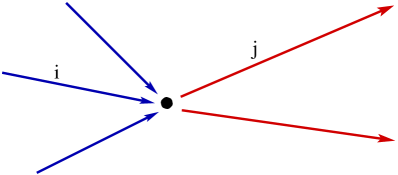
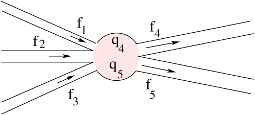
Consider an intersection, say with $m$ incoming roads $i\in\{1,\ldots,m\}={\cal I}$ and $n$ outgoing roads $j\in\{m+1,\ldots,m+n\}={\cal O}$, see Fig. 3. We shall use the space variable $x\in\,]-\infty,\,0]$ for incoming roads and $x\in[0,+\infty[\,$ for outgoing roads. Throughout the following we assume that the density of traffic on each road is governed by a conservation law

$$\rho_{t}+f_{k}(\rho)_{x}~{}=~{}0,\qquad\qquad f_{k}(\rho)\,=\,\rho\,v_{k}(\rho),$$ (2.5)

where the flux function $f_{k}$ satisfies (2.2), for every $k=1,\ldots,m+n$.

Figure 3: An intersection with 3 incoming and 2 outgoing roads.

An appropriate model must depend on various parameters, namely

• $c_{i}$ = relative priority of drivers arriving from road $i$.

• $\theta_{ij}$ = fraction of drivers from road $i$ that turn into road $j$.

For example, if the intersection is regulated by a crosslight, $c_{i}$ could measure the fraction of time when drivers from road $i$ get green light, on average. It is natural to assume

$$c_{i},~{}\theta_{ij}~{}\geq~{}0,\qquad\qquad\sum_{i\in{\cal I}}c_{i}~{}=~{}1,\qquad\qquad\sum_{j\in{\cal O}}\theta_{ij}~{}=~{}1.$$ (2.6)

Boundary conditions should determine the limit values of the traffic density on each of the $m+n$ roads meeting at the intersection:

$$\rho_{i}(t,0-)\,=\,\lim_{x\to 0-}\rho_{i}(t,x),\qquad\rho_{j}(t,0+)\,=\,\lim_{x\to 0+}\rho_{j}(t,x),\qquad\qquad\hbox{for all}~{}i\in{\cal I},~{}j\in{\cal O}.$$ (2.7)

At first sight, one might guess that $m+n$ conditions will be required. However, this is not so, because on some roads the characteristics move toward the intersection. For these roads, the limits in (2.7) are already determined by integrating along characteristics. Boundary conditions are required only for those roads where the characteristics move away from the origin. Recalling the definition of free and congested states, we thus have

$$\begin{array}[]{l}\hbox{[\# of boundary conditions needed to determine the flux at the intersection]}\\[8.53581pt] \quad~{}=~{}\hbox{ [\# of incoming roads which are congested ] + [\# of outgoing roads which are free].}\end{array}$$

It now becomes apparent that, to assign a meaningful set of boundary conditions, several different cases must be considered.

To circumvent these difficulties, an alternative approach developed by Coclite, Garavello, and Piccoli [15, 20, 21] relies on the construction of a Riemann Solver. Instead of assigning a variable number of boundary conditions, here the idea is to introduce a rule for solving all Riemann problems (i.e. the initial-value problems where at time $t=0$ the densities $\rho_{k}$ and turning preferences $\theta_{ij}$ are constant along each road). Relying on front-tracking approximations, under suitable conditions one can prove that the solutions with general initial data are also uniquely determined. We briefly review the main steps of this construction, for the constant initial data

$$\left\{\begin{array}[]{l}\rho_{1},\ldots,\rho_{m},\rho_{m+1},\ldots\rho_{m+n}~{}=~{}\hbox{initial densities on the incoming and outgoing roads,}\cr\theta_{ij}~{}=~{}\hbox{fraction of drivers from road $i$ that turn into road $j$.}\end{array}\right.$$

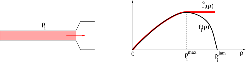
Step 1. Determine the maximum flux $f_{i}^{max}$ that can exit from each incoming road $i\in{\cal I}$.

As shown in Fig. 4, this is computed by

$$f_{i}^{max}~{}=~{}\widehat{f}_{i}(\rho_{i})~{}=~{}\left\{\begin{array}[]{cl}f_{i}(\rho_{i})&\hbox{if}\qquad\rho_{i}\leq\rho_{i}^{max},\\[8.53581pt] f_{i}(\rho_{i}^{max})&\hbox{if}\qquad\rho_{i}>\rho_{i}^{max}\,.\end{array}\right.$$

Figure 4: Computing the maximum flux that can come out from a road $i\in{\cal I}$.

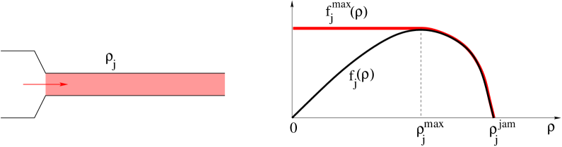
Step 2: Determine the maximum flux $f_{j}^{max}$ that can enter each outgoing road $j\in{\cal O}$.

As shown in Fig. 5, this is computed by

$$f_{j}^{max}~{}=~{}\widehat{f}_{j}(\rho_{j})~{}=~{}\left\{\begin{array}[]{cl}f_{j}(\rho_{j})&\hbox{if}\qquad\rho_{i}\geq\rho_{i}^{max},\\[8.53581pt] f_{j}(\rho_{j}^{max})&\hbox{if}\qquad\rho_{j}<\rho_{j}^{max}\,.\end{array}\right.$$

Figure 5: Computing the maximum flux that can get into a road $j\in{\cal O}$.

Step 3: Given the maximum incoming and outgoing fluxes $f_{i}^{max}$, $f_{j}^{max}$, and the turning preferences $\theta_{ij}$, determine the region of admissible incoming fluxes

$$\Omega~{}\doteq~{}\left\{(f_{1},\ldots,f_{m})\,;~{}~{}f_{i}\in[0,f_{i}^{max}],\qquad\sum_{i\in{\cal I}}f_{i}\theta_{ij}\leq f_{j}^{max}\quad\hbox{for all}~{}j\in{\cal O}\right\}.$$ (2.8)

Figure 6: The region $\Omega\subset I\!\!R^{m}$ of admissible incoming fluxes, defined at (2.8).

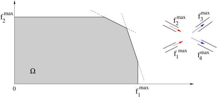
Step 4. To construct a Riemann solver, it now suffices to give a rule for selecting a point $\bar{\omega}=(f_{1},\ldots,f_{m})$ in the feasible region $\Omega$. In general, this rule will depend on the priority coefficients $c_{1},\ldots,c_{m}$ assigned to incoming roads. Observe that, as soon as the incoming fluxes $f_{i}$, $i\in{\cal I}$, are given, the outgoing fluxes are uniquely determined by the identities

$$f_{j}~{}=~{}\sum_{i\in{\cal I}}f_{i}\theta_{ij}\,,\qquad\qquad j\in{\cal O}.$$ (2.9)

Various ways to define a Riemann Solver are illustrated by the following examples. Example 1: Given priority coefficients $c_{1},\ldots,c_{m}$, following [15] one can choose the vector of incoming fluxes

$$\bar{\omega}~{}=~{}(f_{1},\ldots,f_{m})~{}\doteq~{}\hbox{arg}\!\max_{\omega\in\Omega}~{}\sum_{i\in{\cal I}}c_{i}f_{i}\,.$$ (2.10)

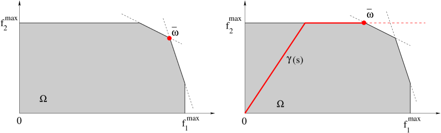
In particular, if $c_{1}=\cdots=c_{m}={1\over m}$, this means we are maximizing the total flux through the intersection (see Fig. 7, left). Since in (2.10) we are maximizing a linear function over a polytope, in some cases the maximum can be attained at multiple points. This somewhat restricts the applicability of this model. An alternative model, with better continuity properties, is considered below. Example 2: Given positive coefficients $c_{1},\ldots,c_{m}$ as in (2.6), consider the one-parameter curve

$$s~{}\mapsto~{}\gamma(s)~{}=~{}(\gamma_{1}(s),\ldots,\gamma_{m}(s)),$$

where

$$\gamma_{i}(s)~{}\doteq~{}\min\{c_{i}s\,,~{}f_{i}^{max}\}.$$

As shown in Fig. 7, right, we then choose the vector of incoming fluxes

$$\overline{\omega}~{}=~{}(f_{1},\ldots,f_{m}),\qquad\qquad f_{i}~{}=~{}\gamma_{i}(\bar{s}),$$ (2.11)

where

$$\bar{s}~{}=~{}\max~{}\left\{s\geq 0\,;~{}~{}\sum_{i\in{\cal I}}\gamma_{i}(s)\,\theta_{ij}~{}\leq~{}f_{j}^{max}\quad\hbox{for all}~{}j\in{\cal O}\right\}.$$ (2.12)

Figure 7: Left: the point $\bar{\omega}\in\Omega$ which maximizes the total flux through the intersection. Right: the point $\bar{\omega}\in\Omega$ constructed by the Riemann Solver at (2.11)-(2.12).

Figure 8: A Riemann Solver modeling an intersection where the second road has a stop sign.

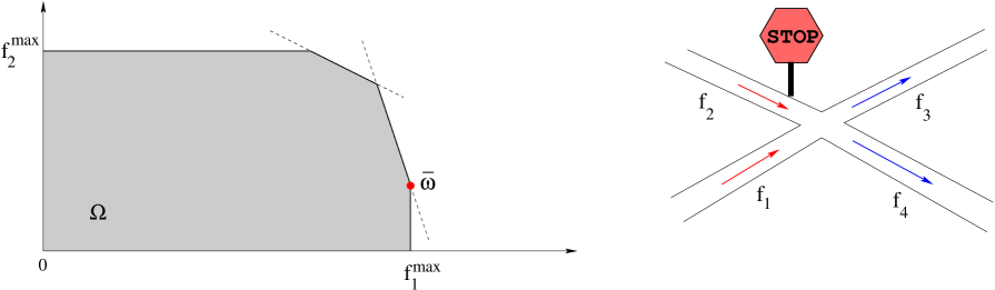
Example 3 : To model an intersection with two incoming and two outgoing roads, where road 2 has a stop sign, we choose the point $\overline{\omega}=(f_{1},f_{2})$ according to the following rules (see Fig. 8).

$$f_{1}~{}=~{}\max~{}\{\omega_{1}\,;~{}~{}(\omega_{1},0)\in\Omega\}.$$ (2.13)

$$f_{2}~{}=~{}\left\{\begin{array}[]{cl}0&\hbox{if}\quad f_{1}<f_{1}^{max},\\[8.53581pt] \max~{}\{\omega_{2}\,;~{}~{}(f_{1},\omega_{2})\in\Omega\}&\hbox{if}\quad f_{1}=f_{1}^{max}\end{array}\right.$$ (2.14)

According to (2.13), as many cars as possible are allowed to arrive from road 1. According to (2.14), if any available space is left, cars arriving from road 2 are allowed through the intersection.

2.3 Intersection models with buffers.

Having defined a way to solve each Riemann problem, a major issue is whether the Cauchy problem with general initial data is well posed. Assuming that the turning preferences $\theta_{ij}$ remain constant in time, some results in this direction can be found in [15].

We remark, however, that in general these turning preferences may well vary in time. One should thus regard $\theta_{ij}=\theta_{ij}(t,x)$ as variables. Assuming that drivers know in advance their itinerary, the conservation of the number of drivers on road $i$ that will eventually turn into road $j$ is expressed by the additional conservation law

$$[\rho_{i}\theta_{ij}]_{t}+[\rho_{i}v_{i}(\rho)\theta_{ij}]_{x}~{}=~{}0.$$ (2.15)

Combining (2.15) with the conservation law

$$(\rho_{i})_{t}+[\rho_{i}v_{i}(\rho)]_{x}~{}=~{}0,$$

one obtains a linear transport equation for each of the quantities $\theta_{ij}$, namely

$$(\theta_{ij})_{t}+v_{i}(\rho)\,(\theta_{ij})_{x}~{}=~{}0,\qquad\qquad i\in{\cal I},~{}~{}j\in{\cal O}.$$ (2.16)

A surprising counterexample constructed in [14] shows that, for a very general class of Riemann Solvers, one can construct measurable initial data $\rho_{i}(0,\cdot)$, $\rho_{j}(0,\cdot)$, and $\theta_{ij}(0,\cdot)$, so that the Cauchy problem has two distinct entropy-admissible solutions.

The ill-posedness of these model equations represents a serious obstruction, toward the existence of globally optimal traffic patterns, or Nash equilibria, on a general network of roads. To cope with this difficulty, in [10] an alternative model was proposed, for traffic flow at an intersection. Namely, it is assumed that the junction contains a buffer (say, a traffic circle). Incoming cars are admitted at a rate depending of the amount of free space left in the buffer, regardless of their destination. Once they have entered the intersection, cars flow out at the maximum rate allowed by the outgoing road of their choice.

More precisely, consider a constant $M>0$, describing the maximum number of cars that can occupy the intersection at any given time, and constants $c_{i}>0$, $i\in{\cal I}$, accounting for priorities given to different incoming roads. For $j\in{\cal O}$, at any time $t$ we denote by $q_{j}(t)\in[0,M]$ the number of cars, already within the buffer, that seek to turn into road $j$.

As before, let $f_{i}^{max}$ and $f_{j}^{max}$ the maximum fluxes that can exit from road $i\in{\cal I}$, or can enter into road $j\in{\cal O}$. We then require that the incoming fluxes $f_{i}$ satisfy

$$f_{i}~{}=~{}\min~{}\left\{f^{max}_{i}\,,~{}~{}c_{i}\Big{(}M-\sum_{j\in{\cal O}}q_{j}\Big{)}\right\},\qquad\qquad i\in{\cal I}\,.$$ (2.17)

In addition, the outgoing fluxes $f_{j}$ should satisfy

$$\left\{\begin{array}[]{l}\hbox{if $q_{j}>0$, then $f_{j}=f^{max}_{j}$,}\cr\cr\hbox{if $q_{j}=0$, then $f_{j}=\min\Big{\{}f^{max}_{j},~{}\sum_{i\in{\cal I}}f_{i}\theta_{ij}\Big{\}}$,}\end{array}\right.\qquad\qquad j\in{\cal O}\,.$$ (2.18)

Having determined the incoming and outgoing fluxes $f_{i}$, $f_{j}$, the time derivatives of the queues $q_{j}$ are then computed by

$$\dot{q}_{j}~{}=~{}\sum_{i\in{\cal I}}f_{i}\theta_{ij}-f_{j}\,,\qquad\qquad j\in{\cal O}.$$ (2.19)

The well-posedness of the intersection model with buffers, for general ${\bf L}^{\infty}$ data, was proved in [10].

It is interesting to understand the relation between the intersection model with buffer, and the models based on a Riemann Solver. The analysis in [12] shows that, letting the size of the buffer $M\to 0$, the solution of the problem with buffers converges to the solution determined by the Riemann Solver at (2.11)-(2.12), described in Example 2.

Figure 9: An intersection model with a buffer. Here the queue sizes $q_{4},q_{5}$ account for the number of cars that have already accessed the intersection, and are waiting to exit into roads 4 and 5 respectively.

2.4 Optima and equilibria on a network of roads.

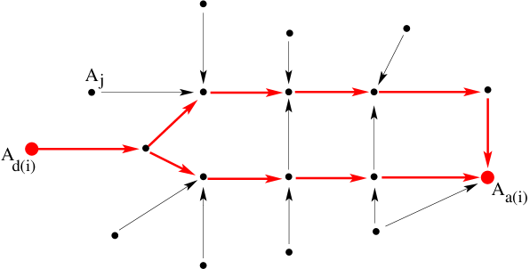
Consider a network of roads, with several intersections. We call $\gamma_{k}$, $k=1,\ldots,\bar{k}$ the arcs corresponding to the various roads, and $A_{1},\ldots,A_{\nu}$ the nodes corresponding to intersections. It is assumed that, on the $k$-th road, the flux function has the form $f_{k}(\rho)=\rho\,v_{k}(\rho)$, with $v_{k}$ a decreasing function of the density. As in the previous sections, traffic flow at each intersection can be modeled in terms of a Riemann Solver, or by means of a buffer.

We consider $N$ groups of drivers with different origins and destinations, and possibly different departure and arrival costs. As shown in Fig. 10:

• Drivers in the $i$-th group depart from the node $A_{d(i)}$ and arrive at the node $A_{a(i)}$.

• Their cost for departing at time $t$ is $\varphi_{i}(t)$, while their arrival cost is $\psi_{i}(t)$.

• They can use different paths $\Gamma_{1},\Gamma_{2},\ldots$ to reach destination.

Figure 10: A network of roads, with several intersections at nodes $A_{j}$. Drivers of the $i$-th group depart from the node $A_{d(i)}$ and arrive to node $A_{a(i)}$. In this example they can choose two distinct paths to reach destination.

In the following, $\bar{u}_{i,p}(\cdot)$ will denote the departure rate of drivers of the $i$-th group, who choose the path $\Gamma_{p}$ to reach destination. Calling $G_{i}$ the total number of drivers in the $i$-th group, we say that the departure rates $\bar{u}_{i,p}$ are admissible if, for every $i=1,\ldots,N$ they satisfy the obvious constraints

$$\bar{u}_{i,p}(t)~{}\geq~{}0,\qquad\qquad\sum_{p}\int_{-\infty}^{+\infty}\bar{u}_{i,p}(t)\,dt~{}=~{}G_{i}\,.$$ (2.20)

Given the departure rates, in principle one can then solve the equation of traffic flow on the whole network and determine the arrival times of the various drivers. We call

$$\tau_{p}(t)~{}=~{}\hbox{arrival time of a driver departing at time $t$, traveling along the path $\Gamma_{p}$.}$$

With these notations, we can introduce

Definition 2.1

An admissible family $\{\bar{u}_{i,p}\}$ of departure rates is globally optimal if it minimizes the sum of the total costs of all drivers

$$J(\bar{u})~{}\doteq~{}\sum_{i,p}\int\Big{(}\varphi_{i}(t)+\psi_{i}(\tau_{p}(t))\Big{)}\bar{u}_{i,p}(t)\,dt\,.$$

Definition 2.2

An admissible family $\{\bar{u}_{k,p}\}$ of departure rates is a Nash equilibrium if no driver of any group can lower his own total cost by changing departure time or switching to a different path to reach destination.

From the above definition it follows the existence of constants $C_{1},\ldots,C_{N}$ such that

$$\begin{array}[]{l}\varphi_{k}(t)+\psi_{k}(\tau_{p}(t))~{}=~{}C_{k}\qquad\qquad\hbox{for all}~{}t\in{\rm Supp}(\bar{u}_{k,p})\,,\cr\cr\varphi_{k}(t)+\psi_{k}(\tau_{p}(t))~{}\geq~{}C_{k}\qquad\qquad\hbox{for all}~{}t\in I\!\!R\,.\end{array}$$

As remarked in the Introduction, a similar characterization for the globally optimal solution is much harder to justify.

Figure 11: A flux function $f_{k}$, a departure cost function $\varphi_{i}$, and and arrival cost function $\psi_{i}$, satisfying the assumptions (A1)-(A2).

In the above setting, a natural set of assumptions is (see Fig. 11)

• On each road $k=1,\ldots,\bar{k}$, the flux function $f_{k}$ satisfies

  $$f_{k}\in{\cal C}^{2},\qquad f_{k}^{\prime\prime}<0,\qquad f_{k}(0)=f_{k}(\rho_{k}^{jam})=0.$$ (2.21)

• For each group of drivers $i=1,\ldots,N$, the cost functions $\varphi_{i}$, $\psi_{i}$ satisfy

  $$\varphi_{i}^{\prime}~{}<~{}0,\qquad\psi_{i},\psi_{i}^{\prime}~{}>~{}0,\qquad\quad\lim_{|t|\to\infty}\Big{(}\varphi_{i}(t)+\psi_{i}(t)\Big{)}~{}=~{}+\infty.$$ (2.22)

When all intersections are modeled in terms of a buffer as in (2.17)–(2.19), under the assumptions (A1), (A2), the existence of at least one globally optimal solution and at least one Nash equilibrium solution was proved in [11].

3 Optimal solutions: a single road, several groups of drivers

Consider a single road, where the traffic density is governed by the conservation law

$$\rho_{t}+f(\rho)_{x}~{}=~{}0\qquad\qquad\text{for}\quad x\in[0,L].$$ (3.1)

We assume that $N$ groups of drivers are present, of sizes $G_{1},\ldots,G_{N}$, with departure and arrival costs $\varphi_{i}$, $\psi_{i}$, $i=1,\ldots,N$. The flux function will be denoted by

$$u(t,x)~{}=~{}f(\rho(t,x))~{}=~{}\sum_{i=1}^{N}u_{i}(t,x).$$

Here

$$u_{i}(t,x)~{}=~{}\theta_{i}(t,x)\,u(t,x)$$ (3.2)

is the flux of drivers of the $i$-th group. As in (2.6), we always assume that

$$\theta_{i}(t,x)\,\geq\,0,\qquad\qquad\sum_{i}\theta_{i}(t,x)\,=\,1.$$ (3.3)

For each $i\in\{1,\ldots,N\}$, the conservation of the number of drivers of the $i$-th family yields the additional conservation law

$$(\rho\theta_{i})_{t}+\Big{(}\rho v(\rho)\,\theta_{i}\Big{)}_{x}~{}=~{}0\,.$$ (3.4)

By (3.1), one obtains the linear equations

$$\theta_{i,t}+v(\rho)\,\theta_{i,x}~{}=~{}0,\qquad\qquad i=1,\ldots,N.$$ (3.5)

The incoming flux at the beginning of the road is

$$u(t,0)~{}=~{}\bar{u}(t)~{}=~{}\sum_{i=1}^{N}\bar{\theta}_{i}(t)\,\bar{u}(t).$$ (3.6)

The global optimization problem can be formulated as follows.

• Given the constants $G_{i}>0$, $i=1,\ldots,N$, find departure rates $\bar{u}_{i}(t)=\bar{\theta}_{i}(t)\bar{u}(t)$ which provide an optimal solution to the problem

  $$\hbox{minimize:}\qquad J(\bar{u}_{1},\ldots,\bar{u}_{N})~{}\doteq~{}\sum_{i=1}^{N}~{}\int_{-\infty}^{+\infty}\Big{[}u_{i}(t,0)\varphi_{i}(t)+u_{i}(t,L)\psi_{i}(t)\Big{]}\,dt,$$ (3.7)

  and satisfy the constraints

  $$\bar{u}(t)\in[0,M],\qquad\bar{\theta}_{i}(t)\,\geq\,0,\qquad\sum_{i=1}^{N}\bar{\theta}_{i}(t)~{}=~{}1,\qquad\hbox{for all}~{}t\in I\!\!R,$$ (3.8)

  $$\bar{u}_{i}(t)\,\geq\,0,\qquad\qquad\int_{-\infty}^{+\infty}\bar{u}_{i}(t)\,dt~{}=~{}G_{i}\,,\qquad\quad i=1,\ldots,N.$$ (3.9)

We recall that $u_{i}(t,L)=\theta_{i}(t,L)u(t,L)$ is the rate at which the drivers of the $i$-th group arrive at the end of the road.

Since no intersections are present, the existence of a globally optimal solution follows as a special case of the result in [11]. Here we briefly recall the main argument in the proof.

1. Let $(\bar{u}_{1}^{(n)},\ldots,\bar{u}_{N}^{(n)})_{n\geq 1}$ be a minimizing sequence of admissible departure rates. Namely

$$\bar{u}^{(n)}_{i}(t)\geq 0,\qquad\qquad\sum_{i=1}^{N}\bar{u}^{(n)}_{i}(t)~{}\leq M,\qquad\qquad\int_{-\infty}^{+\infty}\bar{u}^{(n)}_{i}(t)\,dt~{}=~{}G_{i}$$

for every $n\geq 1$, and moreover

$$\lim_{n\to\infty}~{}J(\bar{u}_{1}^{(n)},\ldots,\bar{u}_{N}^{(n)})~{}=~{}\inf J(\bar{u}_{1},\ldots,\bar{u}_{N}).$$

2. By the assumption (A2), as $t\to\pm\infty$ the cost functions $\varphi_{i},\psi_{i}$ become very large. By possibly modifying the functions $\bar{u}_{i}$, we can thus obtain a minimizing sequence where all departure rates vanish outside a fixed time interval $[a,b]$.

3. By taking a subsequence, we obtain a weak limit $(\bar{u}_{1}^{(n)},\ldots,\bar{u}_{N}^{(n)})\rightharpoonup(\bar{u}_{1},\ldots,\bar{u}_{N})$.

The boundedness of the supports guarantees that these limit departure rates are still admissible (i.e., no mass leaks at infinity).

4. Call $u_{i}^{(n)}(t,x)$, $u_{i}(t,x)$ the corresponding solutions. By the genuine nonlinearity of the conservation law (3.1), after taking a subsequence, one obtains the strong convergence $u^{(n)}(\cdot,L)\to u(\cdot,L)$ in ${\bf L}^{1}(I\!\!R)$, and the weak convergence of the departure and arrival rates

$$u^{(n)}_{i}(\cdot,0)\rightharpoonup u_{i}(\cdot,0),\qquad\qquad u^{(n)}_{i}(\cdot,L)\rightharpoonup u_{i}(\cdot,L).$$

Since the cost functional in (3.7) is linear w.r.t. these departure and arrival rates, it is continuous w.r.t. weak convergence. This yields the optimality of the departure rates $(\bar{u}_{1},\ldots,\bar{u}_{N})$.

3.1 Optimality conditions.

In the remainder of this section, we seek necessary conditions for a solution to be optimal. As a first step, we derive an explicit representation of the solution.

Following [5, 6], it is convenient to switch the roles of the variables $t,x$, and write the density $\rho$ as a function of the flux $u$. The boundary value problem (3.1)-(3.6) thus becomes a Cauchy problem for the conservation law describing the flux $u=\rho v(\rho)$, namely

$$u_{x}+g(u)_{t}~{}=~{}0\,,$$ (3.10)

$$u(t,0)~{}=~{}\bar{u}(t)\,.$$ (3.11)

As shown in Fig. 12, the function $u\mapsto g(u)~{}=~{}\rho$ is defined as a partial inverse of the function $\rho\mapsto\rho\,v(\rho)=u$, assuming that

$$0~{}\leq~{}u~{}\leq~{}M~{}\doteq~{}\max_{\rho\geq 0}\rho v(\rho)\,,\qquad\qquad 0~{}\leq~{}\rho~{}\leq~{}\rho^{max}.$$

For convenience, we extend $g$ to the entire real line by setting

$$g(u)~{}\doteq~{}\left\{\begin{array}[]{cl}g^{\prime}(0+)u&\hbox{if}~{}~{}u<0,\\[8.53581pt] +\infty&\hbox{if}~{}~{}u>M\,.\end{array}\right.$$ (3.12)

The solution to (3.10)-(3.11) can now be expressed by means of the Lax formula [18, 24]. Namely, call

$$g^{*}(p)~{}\doteq~{}\max_{u}\{pu-g(u)\}$$ (3.13)

the Legendre transform of $g$. Notice that

$$g^{*}(p)~{}=~{}+\infty\qquad\hbox{for}\quad p<g^{\prime}(0).$$

On the other hand, for $p\geq g^{\prime}(0)$ the strict convexity of $g$ implies that there exists a unique value $u=\gamma(p)\geq 0$ where the maximum in (3.13) is attained, so that

$$g^{*}(p)~{}=~{}p\cdot\gamma(p)-g(\gamma(p)).$$

This function $\gamma:[g^{\prime}(0),+\infty[\,\mapsto[0,M[\,$ is implicitly defined by the relation

$$g^{\prime}(\gamma(p))~{}=~{}p.$$ (3.14)

Consider the integrated function

$$U(t,x)~{}\doteq~{}\int_{-\infty}^{t}u(\tau,x)\,d\tau,$$

which measures the number of drivers that have crossed the point $x$ along the road before time $t$. The conservation law (3.10) can be equivalently written as a Hamilton-Jacobi equation

$$U_{x}+g(U_{t})~{}=~{}0$$ (3.15)

with data at $x=0$

$$U(t,0)~{}=~{}\overline{U}(t)~{}=~{}\int_{-\infty}^{t}\bar{u}(s)\,ds.$$ (3.16)

The solution to (3.10)-(3.11) is now provided by the Lax formula

$$U(t,x)~{}=~{}\min_{\tau}~{}\left\{xg^{*}\Big{(}{t-\tau\over x}\Big{)}+\overline{U}(\tau)\right\}\,,$$ (3.17)

$$\tau(t,x)~{}\doteq~{}\hbox{arg}\!\min_{\tau}~{}\left\{xg^{*}\Big{(}{t-\tau\over x}\Big{)}+\overline{U}(\tau)\right\}\,,$$ (3.18)

$$u(t,x)~{}=~{}\gamma\left(t-\tau(t,x)\over x\right).$$ (3.19)

We observe that the function $U=U(t,x)$ is globally Lipschitz continuous. Its values satisfy

$$U(t,x)~{}\in~{}[0,G],\qquad\qquad G=G_{1}+\ldots+G_{N}\,.$$ (3.20)

Car trajectories $t\mapsto y(t)$ are defined to be the solutions to the ODE

$$\dot{y}(t)~{}=~{}v(\rho(t,y(t))).$$ (3.21)

In the region where $\rho>0$, and hence $u=\rho v(\rho)>0$ as well, these trajectories coincide with the level curves of the integral function $U$. Indeed, observing that $v=u/\rho$, when $\rho=g(u)>0$ we can write

$$\dot{y}(t)~{}=~{}v(\rho(t,y(t)))~{}=~{}{u(t,y(t))\over g(u(t,y(t))}~{}=~{}{U_{t}(t,y(t))\over g(U_{t}(t,y(t))}\,.$$

By (3.15) one has

$${d\over dt}\,U(t,y(t))~{}=~{}U_{t}+U_{x}\dot{y}(t)~{}=~{}U_{t}+U_{x}\,{U_{t}\over g(U_{t})}~{}=~{}0.$$ (3.22)

More generally, consider a car departing at time $t_{0}$. The solution to the Cauchy problem

$$\dot{y}(t)~{}=~{}v(\rho(t,y(t))),\qquad\quad y(t_{0})\,=\,0$$ (3.23)

can be determined by the formula

$$y(t)~{}=~{}\inf\left\{x\,;~{}~{}U(t,x)>\overline{U}(t_{0})\quad\hbox{or}\quad x={t-t_{0}\over v(0)}\right\}.$$ (3.24)

The arrival time of a driver departing at time $t_{0}$ is

$$\tau^{a}(t_{0})~{}=~{}\sup\left\{t^{\prime}\,;~{}~{}U(t^{\prime},L)<\overline{U}(t_{0})\quad\hbox{or}~{}~{}t^{\prime}=t_{0}+{L\over v(0)}\right\}.$$ (3.25)

By (3.5), the functions $\theta_{i}$ are constant along car trajectories.

In order to compute the arrival rates $u_{i}=\theta_{i}u$ at the terminal point of the road $x=L$, we first observe that the map

$$t~{}\mapsto~{}\overline{U}(t)$$

in (3.16) is nondecreasing. Hence we can define an inverse by setting

$$\overline{\tau}(s)~{}\doteq~{}\inf~{}\{t\in I\!\!R\,;~{}\overline{U}(t)\geq s\}~{}\in~{}\Big{[}0\,,~{}\sum_{i}G_{i}\Big{]}.$$ (3.26)

We then introduce the functions

$$\Theta_{i}(s)~{}\doteq~{}\bar{\theta}_{i}(\bar{\tau}(s))$$ (3.27)

By (3.5), the functions $\theta_{i}=\theta_{i}(t,x)$ are constant along car trajectories. The general solution to (3.5)-(3.6) can thus be written as

$$\theta_{i}(t,x)~{}=~{}\Theta_{i}(U(t,x)).$$ (3.28)

We shall be mostly interested in the terminal values $u(t,L)$, describing the rate at which cars arrive at the end of the road. Denoting the arrival distribution as $U^{a}(t)\doteq U(t,L)$, the total cost can now be written as

$$J~{}=~{}\int\varphi(t)\,d\overline{U}(t)+\sum_{i}\int\psi_{i}(t)\,\Theta_{i}(U^{a}(t))\,dU^{a}(t).$$ (3.29)

Figure 12: Left: the function $\rho\mapsto\rho\,v(\rho)$ describing the flux of cars. Middle: the function $g$, implicitly defined by $g(\rho v(\rho))=\rho$ and extended according to (3.12). Right: the Legendre transform $g^{*}$.

Theorem 3.1

Let the flux function $f$ satisfy the standard assumptions (2.2). Assume that all drivers have the same departure cost $\varphi_{i}=\varphi$ and possibly different arrival costs $\psi_{1},\ldots,\psi_{N}$, satisfying (2.22). Let $(\bar{u}_{1},\ldots,\bar{u}_{N})$ an optimal departure rate, minimizing the total cost to all drivers.

Then the corresponding solution does not contain shocks. Moreover, there exists constants $C_{1},\ldots,C_{N}$ such that, setting

$$\psi(t)~{}\doteq~{}\min_{k}~{}(\psi_{k}(t)-C_{k})\,,$$ (3.30)

the following holds:

• For any $t\in I\!\!R$, let $T(t)$ be the unique time such that

  $$\varphi(t)+\psi(T(t))~{}=~{}0\,.$$ (3.31)

  Then, for every point $(t^{\prime},x^{\prime})$ along the segment with endpoints $(t,0)$ and $(T(t),L)$, one has

  $$u(t^{\prime},x^{\prime})~{}=~{}\left\{\begin{array}[]{cl}\displaystyle\gamma\left({T(t)-t\over L}\right)&\hbox{if}\quad\displaystyle{T(t)-t\over L}\,\geq\,g^{\prime}(0),\\[11.38109pt] 0&\hbox{otherwise}.\end{array}\right.$$ (3.32)

• Calling $u_{i}(\cdot,L)$ the arrival rate of drivers of the $i$-th group, one has

  $$\hbox{Supp}(u_{i}(\cdot,L))~{}\subseteq~{}\{s\,;~{}~{}\psi(s)\,=\,\psi_{i}(s)-C_{i}\}.$$ (3.33)

A proof of Theorem 3.1 will be given in the next section.

4 Proof of the necessary conditions

As a preliminary, we review the basic theory of scalar conservation laws with convex flux [3, 18, 28]. Notice that in (3.10) the usual role of the variables $t,x$ is reversed, because of the particular meaning of the equations.

Let $u=u(t,x)$ be a weak solution to (3.10), taking values within the interval $[0,M]$. This solution is entropy admissible if it contains only downward jumps, namely

$$u(t+,x)~{}\doteq~{}\lim_{s\to t+}u(s,x)~{}\leq~{}\lim_{s\to t-}u(s,x)~{}\doteq~{}u(t-,x).$$

By a generalized characteristic we mean a function $x\mapsto t(x)$ which provides a solution to the differential inclusion

$${d\over dx}t(x)~{}\in~{}\Big{[}g^{\prime}(u(t+,x)),\,g^{\prime}(u(t-,x))\Big{]}.$$ (4.1)

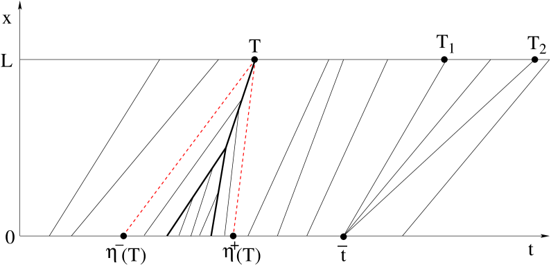
For any given point $(T,L)$, there exists a minimal and a maximal backward characteristic. As shown in Fig. 13, we denote by $(\eta^{-}(T),0)$ and $(\eta^{+}(T),0)$ the initial points of these characteristics. Calling $\overline{U}$ the integral function in (3.17), the points $\eta^{-}(T)$ and $\eta^{+}(T)$ are respectively the minimum and the maximum elements within the set

$$I(T)~{}\doteq~{}\left\{t\in I\!\!R;t=\hbox{arg}\!\min\limits_{\tau}\left\{Lg^{*}\left({T-\tau\over L}\right)+\overline{U}(\tau)\right\}\right\}$$ (4.2)

where the function $\Lambda(t)~{}\doteq~{}Lg^{*}\left({T-t\over L}\right)+\overline{U}(t)$ attains its global minimum.

Two cases can occur:

• The global minimum in (4.2) is attained at a single point $t^{*}=\eta^{-}(T)=\eta^{+}(T)$.

  The function $u(\cdot,L)$ is then continuous at the point $T$, and

  $$u(T,L)~{}=~{}\gamma\left({T-t^{*}\over L}\right).$$

• The global minimum in (4.2) is attained at multiple points, hence $\eta^{-}(T)<\eta^{+}(T)$.

  In this case the solution contains a shock through the point $(T,L)$. Recalling (3.14), the left and right values across the shock are determined by

  $$u(T-,L)~{}=~{}\gamma\left({T-\eta^{-}(T)\over L}\right),\qquad\qquad u(T+,L)~{}=~{}\gamma\left({T-\eta^{+}(T)\over L}\right).$$

We observe that characteristics do not cross each other. Indeed, one has the implication

$$T_{1}\,<\,T_{2}\qquad\Longrightarrow\qquad\eta^{+}(T_{1})\,\leq\,\eta^{-}(T_{2}).$$ (4.3)

From (4.3) it immediately follows that

• The profile $u(\cdot,L)$ can contain at most countably many shocks. Namely, there can be at most countably many points $T_{i}$ such that $\eta^{-}(T_{i})<\eta^{+}(T_{i})$.

• There can be at most countably many points $t_{i}$ such that

  $$t_{i}~{}=~{}\eta^{+}(T_{1})~{}=~{}\eta^{-}(T_{2})\,,$$ (4.4)

  for two distinct points $T_{1}<T_{2}$.

We recall that, given any function $\phi\in{\bf L}^{1}_{loc}(I\!\!R)$, almost every point $t\in I\!\!R$ is a Lebesgue point of $\phi$. By definition, this means

$$\lim_{h\to 0+}{1\over h}\int_{t-h}^{t+h}|\phi(s)-\phi(t)|\,ds~{}=~{}0.$$ (4.5)

As proved in [5], if $t$ is a Lebesgue point of the initial datum $\bar{u}(\cdot)$, then there exists a unique forward characteristic starting at $t$. In particular, $t$ cannot be the center of a rarefaction wave, and there exists a unique point $T$ such that

$$t~{}\in~{}[\eta^{-}(T),\,\eta^{+}(T)].$$ (4.6)

The next lemma is concerned with the stability of the map $T\mapsto\eta^{\pm}(T)$, w.r.t. small perturbations in the initial datum $\bar{u}$.

Lemma 4.1

Let $u=u(t,x)$ be the unique entropy weak solution of (3.10)-(3.11). Assume that $t$ is a Lebesgue point for the initial datum $\bar{u}$, and let $T$ be the unique point such that (4.6) holds. Then, for any $\varepsilon>0$, one can find $\delta,\delta^{\prime}>0$ such that the following holds.

Let $\bar{u}^{\dagger}$ be a second initial datum, with

$$\|\bar{u}^{\dagger}-\bar{u}\|_{{\bf L}^{1}}~{}\leq~{}\delta\,.$$ (4.7)

If we call $u^{\dagger}$ the corresponding solution, and define the maps $(\eta^{\dagger})^{\pm}$ accordingly, then

$$[t-\delta^{\prime},\,t+\delta^{\prime}]~{}\subseteq~{}[(\eta^{\dagger})^{+}(T-\varepsilon),\,(\eta^{\dagger})^{-}(T+\varepsilon)].$$ (4.8)

Proof. 1. Let $\varepsilon>0$ be given. By the uniqueness assumption, for the solution $u$ the backward characteristics through the points $T-\varepsilon$ and $T+\varepsilon$ satisfy

$$\eta^{+}(T-\varepsilon)~{}<~{}t~{}<~{}\eta^{-}(T+\varepsilon).$$

Hence we can find $\delta^{\prime}>0$ such that

$$\eta^{+}(T-\varepsilon)~{}<~{}t-2\delta^{\prime}~{}<~{}t+2\delta^{\prime}~{}<~{}\eta^{-}(T+\varepsilon).$$ (4.9)

2. If the conclusion of the lemma does not hold, we could find a sequence of initial data $\bar{u}_{n}$ with $\|\bar{u}_{n}-\bar{u}\|_{{\bf L}^{1}}\to 0$, such that the corresponding maps $\eta_{n}^{\pm}$ satisfy

$$\eta_{n}^{+}(T-\varepsilon)~{}\geq~{}t-\delta^{\prime}\qquad\hbox{or}\qquad\eta_{n}^{-}(T-\varepsilon)~{}\leq~{}t+\delta^{\prime}.$$ (4.10)

To fix the ideas, assume that the first case holds. Namely, for every $n\geq 1$, there exists $t_{n}\geq t-\delta^{\prime}$ such that

$$Lg^{*}\left({T-\varepsilon-t_{n}\over L}\right)+\overline{U}_{n}(t_{n})~{}=~{}\min_{\tau}\left\{Lg^{*}\left({T-\varepsilon-\tau\over L}\right)+\overline{U}_{n}(\tau)\right\}.$$ (4.11)

By possibly taking a subsequence we can assume $t_{n}\to t^{*}\geq t-\delta^{\prime}$. The uniform convergence $\overline{U}_{n}\to\overline{U}$ now yields

$$Lg^{*}\left({T-\varepsilon-t^{*}\over L}\right)+\overline{U}(t^{*})~{}=~{}\min_{\tau}\left\{Lg^{*}\left({T-\varepsilon-\tau\over L}\right)+\overline{U}(\tau)\right\}.$$ (4.12)

This implies $\eta^{+}(T-\varepsilon)\geq t-\delta^{\prime}$, reaching a contradiction. MM     

Figure 13: Characteristic lines for a solution of (3.10). Here the point $(T,L)$ lies along a shock, and all (generalized) characteristics starting at a point $(t,0)$ with $t\in[\eta^{-}(T),\,\eta^{+}(T)]$ eventually reach $(T,L)$. Notice that there are several characteristics starting from the point $(\bar{t},0)$, which is the center of a rarefaction wave.

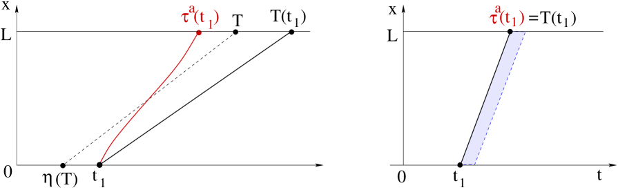
Remark 4.2

As shown in Fig. 13, consider a solution $u=u(t,x)$ containing a shock through the point $(T,L)$. Then we can modify the initial data at $x=0$ inside the interval $[\eta^{-}(T),\eta^{+}(T)]$ so that the solution perturbed solution $u^{\dagger}$ contains a centered compression wave which breaks exactly at $(T,L)$. In view of (3.14), This is achieved by taking

$$\bar{u}^{\dagger}(t)~{}=~{}\left\{\begin{array}[]{cl}\gamma\left({T-t\over L}\right)&\hbox{if}\quad t\in[\eta^{-}(T),\eta^{+}(T)],\\[11.38109pt] \bar{u}(t)&\hbox{if}\quad t\notin[\eta^{-}(T),\eta^{+}(T)].\end{array}\right.$$

This ensures that all characteristics starting at a point $(t,0)$ with $t\in[\eta^{-}(T),\eta^{+}(T)]$ join together at the point $(T,L)$.

Consider the constant

$$\lambda~{}\doteq~{}Lg^{*}\left({T-\eta^{-}(T)\over L}\right)+\overline{U}(\eta^{-}(T))~{}=~{}Lg^{*}\left({T-\eta^{+}(T)\over L}\right)+\overline{U}(\eta^{+}(T)).$$

Then the corresponding integrated function $\overline{U}^{\dagger}$ satisfies

$$Lg^{*}\left({T-t\over L}\right)+\overline{U}^{\dagger}(t)~{}=~{}\lambda\qquad\qquad\hbox{for all}~{}t\in[\eta^{-}(T),\eta^{+}(T)].$$

By (4.2), this implies

$$\overline{U}^{\dagger}(t)~{}\leq~{}\overline{U}(t)\qquad\qquad\hbox{for all}~{}t\in I\!\!R,$$ (4.13)

while the corresponding solutions coincide at $x=L$, namely

$$U^{\dagger}(t,L)~{}=~{}U(t,L),\qquad\qquad u^{\dagger}(t,L)~{}=~{}u(t,L),\qquad\hbox{for all}~{}t\in I\!\!R.$$ (4.14)

Figure 14: Characteristic lines and car trajectories. Here $\tau^{a}(t_{i})$ is the arrival time of a driver departing at time $t_{i}$, while $T(t_{i})$ is the terminal point of the characteristic through $(t_{i},0)$.

The next lemma, analyzing various perturbations to an optimal solution $u$, provides the key step toward the proof of Theorem 3.1.

Lemma 4.3

Let $(\bar{u}_{1},\ldots,\bar{u}_{N})=(\bar{\theta}_{1}\bar{u},\ldots,\bar{\theta}_{N}\bar{u})$ be optimal departure rates. Assume that $t_{1},t_{2}$ are Lebesgue points for all functions $\bar{u},\bar{\theta}_{1},\ldots,\bar{\theta}_{N}$, and

$$\bar{u}(t_{1})\,<\,M,\qquad\qquad\bar{u}_{i}(t_{2})\,>\,0.$$ (4.15)

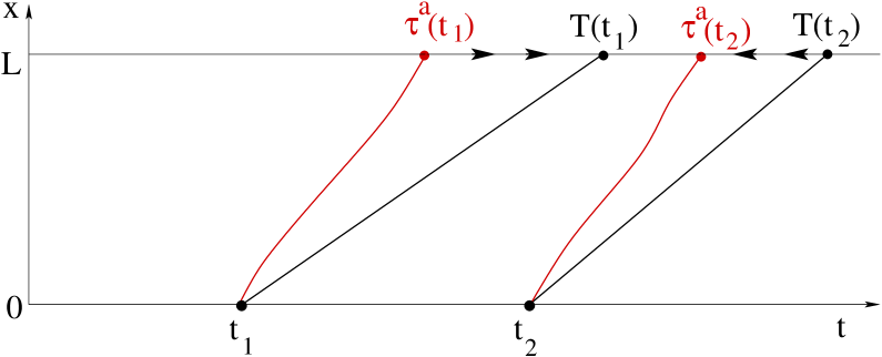
Call $\tau^{a}(t_{1}),\tau^{a}(t_{2})$ the arrival times of a driver departing at times $t_{1},t_{2}$, respectively. Moreover, let $T(t_{1}),T(t_{2})$ be the times where the (unique) generalized forward characteristic starting from $t_{1},t_{2}$ reaches the point $L$. Then

$$\begin{array}[]{l}\displaystyle\varphi(t_{1})+\psi_{i}(\tau^{a}(t_{1}))+\sum_{j=1}^{N}\int_{\tau^{a}(t_{1})}^{T(t_{1})}\psi_{j}^{\prime}(s)\theta_{j}(s,L)\,ds\\[11.38109pt] \qquad\displaystyle\geq~{}\varphi(t_{2})+\psi_{i}(\tau^{a}(t_{2}))+\sum_{j=1}^{N}\int_{\tau^{a}(t_{2})}^{T(t_{2})}\psi_{j}^{\prime}(s)\theta_{j}(s,L)\,ds\,.\end{array}$$ (4.16)

Remark 4.4

The left hand side of (4.16) can be interpreted as the cost for inserting an additional $i$-driver, departing at time $t_{1}$. In this case, an additional driver arrives at time $T(t_{1})$, but this is not the same one! Indeed, the new driver arrives at time $\tau^{a}(t_{1})$. However, the presence of this additional car slows down all the other cars whose arrival time is $T\in[\tau^{a}(t_{1}),\,T(t_{1})]$. The delay in the arrival time of all these cars causes a further increase in the total cost, accounted by the integral term on the left hand side of (4.16). Similarly, the right hand side is the amount which can be saved by removing an $i$-driver departing at time $t_{2}$.

Proof of Lemma 4.3. 1. Since $t_{1},t_{2}$ are Lebesgue points of $\bar{u}$, they cannot be the center of a rarefaction wave. Hence there exist unique points $T_{1}=T(t_{1})$ and $T_{2}=T(t_{2})$ such that

$$t_{i}~{}=~{}\hbox{arg}\!\min_{\tau}~{}\left\{Lg^{*}\Big{(}{T_{i}-\tau\over L}\Big{)}+\overline{U}(\tau)\right\},\qquad\qquad i=1,2.$$ (4.17)

Assuming that (4.16) fails, we shall derive a contradiction. Indeed, we will construct a new initial data $\bar{u}_{i}^{\dagger}$ which is slightly smaller than $\bar{u}_{i}$ in a neighborhood of $t_{1}$ and slightly larger than $\bar{u}_{i}$ in a neighborhood of $t_{2}$, yielding a lower total cost. Various cases can arise, depending on the relative position of $\tau^{a}(t_{i})$ and $T(t_{i})$. To fix the ideas, in the following we assume that

$$\tau^{a}(t_{1})~{}<~{}T(t_{1})~{}<~{}\tau^{a}(t_{2})~{}<~{}T(t_{2}),$$ (4.18)

as shown in Fig. 14. The other cases are handled in a similar way.

We observe that the above strict inequalities imply that $u(\cdot,L)$ is strictly positive on the intervals $[\tau^{a}(t_{1}),T(t_{1})]$ and $[\tau^{a}(t_{2}),T(t_{2})]$. Indeed, the car speed is always $\leq v(0)={1\over g^{\prime}(0)}$. As shown in Fig. 15, if

$${\tau^{a}(t_{1})-t_{1}\over L}~{}=~{}{1\over v(0)}~{}=~{}g^{\prime}(0),$$

then the car speed would be identically equal to the maximum speed $v(0)$. In this case the car trajectory coincides with a characteristic line, and hence $T(t_{1})=\tau^{a}(t_{1})$, against the assumption (4.18). Therefore, we must have

$${\tau^{a}(t_{1})-t_{1}\over L}~{}>~{}g^{\prime}(0)\,,\qquad\qquad\tau^{a}(t_{1})-{L\over v(0)}~{}<~{}t_{1}\,.$$

Since characteristics do not cross each other, for every $T\in\,]\tau^{a}(t_{2}),T(t_{2})[\,$ the initial point of a characteristic through $(T,L)$ must satisfy

$$\eta(T)~{}=~{}T-L\cdot g^{\prime}(u(T,L))~{}\leq~{}t_{1}\,.$$

Hence

$$g^{\prime}(u(T,L))~{}\geq~{}{T-t_{1}\over L}~{}\geq~{}{\tau^{a}(t_{1})-t_{1}\over L}>~{}g^{\prime}(0).$$ (4.19)

Since $g^{\prime}$ is an increasing function, this yields a lower bound on $u(T,L)$.

Figure 15: Left: if $\tau^{a}(t_{1})<T(t_{1})$, the function $u(\cdot,L)$ must be strictly positive on the entire interval $[\tau^{a}(t_{1}),T(t_{1})]$. Right: if $\tau^{a}(t_{1})=T(t_{1})$, then the characteristic and the car trajectory starting at $(t_{1},0)$ coincide, and $u=0$ along this line. A small perturbation in the initial data, supported on $[t_{1},t_{1}+\delta]$, will modify the solution only in a small neighborhood of this characteristic.

2. Consider a perturbed set of initial data of the form $(\bar{u}_{1},\ldots,\bar{u}_{i}^{\dagger},\ldots,\bar{u}_{N})$, where only the component $\bar{u}_{i}$ is modified. The new departure rate for drivers of the $i$-th group is chosen so that

$$\left\{\begin{array}[]{cl}\bar{u}_{i}^{\dagger}(t)~{}=~{}\bar{u}_{i}(t)&\hbox{if}~{}~{}t\notin[t_{1}\,,~{}t_{1}+\delta^{\prime}]\cup[t_{2}\,,~{}t_{2}+\delta^{\prime}]\,,\\[8.53581pt] \bar{u}_{i}^{\dagger}(t)~{}\geq~{}\bar{u}_{i}(t)&\hbox{if}~{}~{}t\in[t_{1}\,,~{}t_{1}+\delta^{\prime}]\,,\\[8.53581pt] 0\,\leq\,\bar{u}_{i}^{\dagger}(t)~{}\,\leq\,\bar{u}_{i}(t)&\hbox{if}~{}~{}t\in[t_{2}\,,~{}t_{2}+\delta^{\prime}]\,,\\[8.53581pt] \end{array}\right.$$ (4.20)

$$\int_{t_{1}}^{t_{1}+\delta^{\prime}}\Big{[}\bar{u}^{\dagger}_{i}(s)-\bar{u}_{i}(s)\Big{]}\,ds~{}=~{}\int_{t_{2}}^{t_{2}+\delta^{\prime}}\Big{[}\bar{u}_{i}(s)-\bar{u}^{\dagger}_{i}(s)\Big{]}\,ds~{}=~{}\delta~{}>~{}0\,.$$ (4.21)

Given $\varepsilon>0$, according to Lemma 4.1, we can choose $\delta,\delta^{\prime}>0$ small enough so that the perturbation in the initial datum

$$u(t,0)~{}=~{}\bar{u}(t)~{}=~{}\sum_{i=1}^{N}\bar{u}_{i}(t)$$

affects the values of $u(\cdot,L)$ only in a small neighborhood of the points $T(t_{1}),T(t_{2})$, namely

$$u^{\dagger}(t,L)~{}=~{}u(t,L)\qquad\qquad\hbox{for all}~{}t\notin[T(t_{1})-\varepsilon\,,~{}T(t_{1})+\varepsilon]\cup[T(t_{2})-\varepsilon\,,~{}T(t_{2})+\varepsilon].$$ (4.22)

3. We now consider a sequence of perturbations of the form (4.20)-(4.21), with $\varepsilon_{n},\delta_{n},\delta^{\prime}_{n}\to 0$. Calling $\tau^{a}_{n}(t)$ the corresponding arrival times, we claim that the following holds.

• Let $t$ be a Lebesgue point for $\bar{u}$, with $\bar{u}(t)>0$, and let $\tau^{a}(t)$ be a Lebesgue point for $u(\cdot,L)$. Then $u(\tau^{a}(t),L)>0$ and the following implications hold.

  $$\tau^{a}(t_{1})~{}<~{}\tau^{a}(t)~{}<~{}T_{1}\qquad\Longrightarrow\qquad\lim_{n\to\infty}{\tau^{a}_{n}(t)-\tau^{a}(t)\over\delta_{n}}~{}=~{}{1\over u(\tau^{a}(t),L)}\,,$$ (4.23)

  $$\tau^{a}(t_{2})~{}<~{}\tau^{a}(t)~{}<~{}T_{2}\qquad\Longrightarrow\qquad\lim_{n\to\infty}{\tau^{a}_{n}(t)-\tau^{a}(t)\over\delta_{n}}~{}=~{}-{1\over u(\tau^{a}(t),L)}\,,$$ (4.24)

  $$\tau^{a}(t)~{}\notin~{}[\tau^{a}(t_{1}),T_{1}]\cup[\tau^{a}(t_{2}),T_{2}]\qquad\Longrightarrow\qquad\lim_{n\to\infty}{\tau^{a}_{n}(t)-\tau^{a}(t)\over\delta_{n}}~{}=~{}0.$$ (4.25)

In first approximation, the above limits show that:

• For those drivers who were reaching destination at a time $T\in\,]\tau^{a}(t_{1}),T_{1}[\,$, the arrival time is delayed by $\delta_{n}/u(\tau^{a}(t),L)$.

• For those drivers who were reaching destination at a time $T\in\,]\tau^{a}(t_{2}),T_{2}[\,$, the arrival time is anticipated by $\delta_{n}/u(\tau^{a}(t),L)$.

• For all other drivers, the arrival time does not change.

To prove the above claim we first observe that, if $u(\tau^{a}(t),L)=0$, then $u(t^{\prime},x^{\prime})=0$ along the backward characteristic

$$\{(t^{\prime},x^{\prime})\,;~{}~{}x^{\prime}~{}=~{}L-(\tau^{a}(t)-t^{\prime})v(0)\}.$$

but in this case, this characteristic coincides with a car trajectory. Hence $\bar{u}(t)=u(0,t)=0$ as well, contradicting our first assumption.

To prove (4.23), assume $\tau^{a}(t_{1})<\tau^{a}(t)<T_{1}$. Then, for all $n$ large enough, the arrival time $\tau^{a}_{n}(t)$ is uniquely determined by the identity

$$U(\tau_{n}^{a}(t),L)~{}=~{}U(\tau^{a}(t),L)+\delta_{n}\,.$$ (4.26)

Observing that the partial derivative is

$${\partial\over\partial\tau}U(\tau,L)\bigg{|}_{\tau=\tau^{a}(t)}~{}=~{}u(\tau^{a}(t),L),$$

from (4.26) one obtains (4.23). Notice that here the denominator is uniformly positive, as a consequence of (4.19).

The proof of (4.24) is entirely similar, replacing (4.26) with the identity

$$U(\tau_{n}^{a}(t),L)~{}=~{}U(\tau^{a}(t),L)-\delta_{n}\,.$$ (4.27)

Finally, if the condition on the left hand side of (4.25) holds, then for all $n\geq 1$ sufficiently large one has $\tau_{n}^{a}(t)=\tau^{a}(t)$, and the implication is trivial. 4. By the properties (4.23) it follows

$$\begin{array}[]{l}\displaystyle\lim_{n\to\infty}~{}{1\over\delta_{n}}\sum_{j=1}^{N}\int_{\tau^{a}(t)\in\,]\tau^{a}(t_{1}),T_{1}[}[\psi_{j}(\tau^{a}_{n}(t))-\psi_{j}(\tau^{a}(t))]\,\bar{u}_{j}(t)\,dt\\[11.38109pt] \qquad=~{}\displaystyle\sum_{j=1}^{N}\int_{\tau^{a}(t)\in\,]\tau^{a}(t_{1}),T_{1}[}\psi^{\prime}_{j}(\tau^{a}(t))\cdot\lim_{n\to\infty}{\tau_{n}^{a}(t)-\tau_{a}(t)\over\delta_{n}}\,\bar{u}_{j}(t)\,dt\\[11.38109pt] \qquad=~{}\displaystyle\sum_{j=1}^{N}\int_{\tau^{a}(t_{1})}^{T_{1}}\psi^{\prime}_{j}(\tau)\cdot{1\over u(\tau,L)}\,u_{j}(\tau,L)\,d\tau\\[11.38109pt] \qquad=~{}\displaystyle\sum_{j=1}^{N}\int_{\tau^{a}(t_{1})}^{T_{1}}\psi^{\prime}_{j}(\tau)\,\theta_{j}(\tau,L)\,d\tau\,.\end{array}$$

An entirely similar computation can be performed on the interval $]\tau^{a}(t_{2}),T_{2}[\,$. Combining these estimates, we thus conclude

$$\begin{array}[]{l}\displaystyle\lim_{n\to\infty}~{}{J(\bar{u}_{1},\ldots,\bar{u}_{i}^{\dagger},\ldots,\bar{u}_{N})-J(\bar{u}_{1},\ldots,\bar{u}_{i},\ldots,\bar{u}_{N})\over\delta_{n}}\\[11.38109pt] \qquad=~{}\displaystyle\varphi(t_{1})+\psi_{i}(\tau^{a}(t_{1}))+\sum_{j=1}^{N}\int_{\tau^{a}(t_{1})}^{T(t_{1})}\psi_{j}^{\prime}(s)\theta_{j}(s,L)\,ds\\[11.38109pt] \qquad\displaystyle-\left[\varphi(t_{2})+\psi_{i}(\tau^{a}(t_{2}))+\sum_{j=1}^{N}\int_{\tau^{a}(t_{2})}^{T(t_{2})}\psi_{j}^{\prime}(s)\theta_{j}(s,L)\,ds\right].\end{array}$$ (4.28)

If the inequality (4.16) does not hold, then the right hand side of (4.28) is negative. This yields a contradiction with the optimality of the departure rates $(\bar{u}_{1},\ldots,\bar{u}_{i},\ldots,\bar{u}_{N})$. 5. The above analysis proves the lemma in the case where (4.18) holds. On the other hand, if $T(t_{1})=\tau^{a}(t_{1})$, then a small perturbation of the departure rate on the interval $[t_{1},t_{1}+\delta_{n}]$ will modify the arrival rate only in a small neighborhood of $\tau^{a}(t_{1})$ (see Fig. 15, right). In this case, one directly proves that the limit (4.28) remains valid, since the integral over the interval $[\tau^{a}(t_{1}),\,T(t_{1})]$ trivially vanishes. MM     

4.1 Proof of Theorem 3.1.

Let $u_{i}(t,0)=\bar{\theta}_{i}(t)\bar{u}(t)$ be optimal departure rates, and let $u$, $\theta_{i}$ be the corresponding solutions to

$$u_{x}+g(u)_{t}~{}=~{}0,\qquad\qquad\theta_{i,t}+v(g(u))\theta_{i,x}~{}=~{}0,\qquad i=1,\ldots,N.$$ (4.29)

The proof will be worked out in several steps. 1. We begin by showing that an optimal solution no shock can occur in the interior of the domain, i.e. for $0\leq x<L$.

Indeed, assume on the contrary that a shock is present, and let $(T,L)$ be the terminal position of this shock. According to Remark 4.2, we can change the initial datum so that the new solution $u^{\dagger}$ contains a centered compression wave focusing at $(T,L)$. More precisely, define $\overline{U}^{\dagger}$, $\bar{u}^{\dagger}$ as in Remark 4.2. Assuming that the functions $\Theta_{i}(s)$ are defined by

$$\overline{U}_{i}(t)~{}\doteq~{}\Theta_{i}(\overline{U}(t))\cdot\overline{U}(t),$$ (4.30)

define the components $(\overline{U}^{\dagger}_{1},\ldots,\overline{U}^{\dagger}_{N})$ by setting

$$\overline{U}_{i}^{\dagger}(t)~{}\doteq~{}\Theta_{i}(\overline{U}^{\dagger}(t))\cdot\overline{U}^{\dagger}(t).$$ (4.31)

Notice that these definition imply

$$U_{i}^{\dagger}(t,L)~{}=~{}U_{i}(t,L)\qquad\qquad\hbox{for all}~{}t\in I\!\!R,$$

hence the arrival costs remain the same. On the other hand, we have

$$\overline{U}_{i}^{\dagger}(t)~{}\leq~{}\overline{U}_{i}(t),$$ (4.32)

for all $i,t$. Observing that there exists some $i$ and some $t\in[\eta^{-}(T),\,\eta^{+}(T)]$ where (4.32) is satisfied as a strict inequality, we claim that the total departure cost for the perturbed solution is strictly smaller.

To see this, introduce a variable $\xi\in[0,G_{i}]$ labeling drivers of the $i$-th group. Define the departure times

$$t_{i}(\xi)~{}\doteq~{}\inf\{t\,;~{}~{}\overline{U}_{i}(t)>\xi\},\qquad\quad t^{\dagger}_{i}(\xi)~{}\doteq~{}\inf\{t\,;~{}~{}\overline{U}^{\dagger}_{i}(t)>\xi\}.$$ (4.33)

By the previous definitions it follows

$$t_{i}(\xi)~{}\leq~{}t_{i}^{\dagger}(\xi),$$

with strict inequality holding at least for some index $i$ and some values of $\xi\in[0,G_{i}]$. We now compute

$$\sum_{i}\int\varphi(t)d\overline{U}_{i}^{\dagger}(t)~{}=~{}\sum_{i}\int_{0}^{G_{i}}\varphi(t_{i}^{\dagger}(\xi))\,d\xi~{}<~{}\sum_{i}\int_{0}^{G_{i}}\varphi(t_{i}(\xi))\,d\xi~{}=~{}\sum_{i}\int\varphi(t)d\overline{U}_{i}(t),$$

proving our claim. 2. Next, we claim that an optimal departure rate satisfies

$$\bar{u}(t)~{}<~{}M\qquad\quad\hbox{for all}~{}t\in I\!\!R.$$ (4.34)

Indeed, since the characteristic speed satisfies $g^{\prime}(u)\to+\infty$ as $u\to M$, if $\bar{u}(\tau)=M$ at some point $\tau$ then the solution $u(\cdot,x)$ would immediately contain a shock, for every $x>0$. By the previous step, this contradicts the optimality assumption. 3. According to Lemma 4.3, by (4.34), the quantity

$$\Delta J(i,t)~{}=~{}\varphi(t)+\psi_{i}(\tau^{a}(t))+\sum_{j=1}^{N}\int_{\tau^{a}(t)}^{T(t)}\psi_{j}^{\prime}(s)\,\theta_{j}(s,L)\,ds$$ (4.35)

is equal to some constant $C_{i}$ for all $t\in{\rm Supp}(\bar{u}_{i})$, and is greater or equal to $C_{i}$ for all $t\in I\!\!R$. In other words, for each $i=1,\ldots,N$ we have

$$\varphi(t)+\psi_{i}(\tau^{a}(t))-C_{i}+\sum_{j=1}^{N}\int_{\tau^{a}(t)}^{T(t)}\psi_{j}^{\prime}(s)\,\theta_{j}(s,L)\,ds~{}=~{}0\qquad\hbox{for all}~{}t\in\hbox{Supp}(\bar{u}_{i})\,,$$ (4.36)

$$\varphi(t)+\psi_{i}(\tau^{a}(t))-C_{i}+\sum_{j=1}^{N}\int_{\tau^{a}(t)}^{T(t)}\psi_{j}^{\prime}(s)\,\theta_{j}(s,L)\,ds~{}\geq~{}0\qquad\hbox{for all}~{}t\in I\!\!R.$$ (4.37)

This implies

$$\varphi(t)+\psi_{i}(\tau^{a}(t))-C_{i}~{}=~{}\varphi(t)+\min_{j}\Big{(}\psi_{j}(\tau^{a}(t))-C_{j}\Big{)}~{}=~{}-\sum_{j=1}^{N}\int_{\tau^{a}(t)}^{T(t)}\psi_{j}^{\prime}(s)\,\theta_{j}(s,L)\,ds$$ (4.38)

for all $t\in\hbox{Supp}(\bar{u}_{i})$. We now observe that, for a.e. $s\in[\tau^{a}(t),T(t)]$ and $j\in\{1,\ldots,N\}$, one has the implication

$$\theta_{j}(s,L)\,>\,0\qquad\Longrightarrow\qquad\psi_{j}(s)-C_{j}~{}=~{}\min_{k}(\psi_{k}(s)-C_{k}).$$ (4.39)

Moreover, for every $j,k$ and a.e. $s$ in the set

$$\bigl{\{}s\in I\!\!R\,;~{}~{}\psi_{j}(s)-C_{j}=\psi_{k}(s)-C_{k}\bigr{\}},$$

one has $\psi_{j}^{\prime}(s)=\psi_{k}^{\prime}(s)$. Therefore, defining $\psi$ as in (3.30) and recalling that $\sum_{j}\theta_{j}=1$, we obtain

$$\sum_{j=1}^{N}\int_{\tau^{a}(t)}^{T(t)}\psi_{j}^{\prime}(s)\,\theta_{j}(s,L)\,ds~{}=~{}\int_{\tau^{a}(t)}^{T(t)}\psi^{\prime}(s)\,ds.$$ (4.40)

In turn, this implies

$$\begin{array}[]{l}\displaystyle\varphi(t)+\psi_{i}(\tau^{a}(t))-C_{i}+\sum_{j=1}^{N}\int_{\tau^{a}(t)}^{T(t)}\psi_{j}^{\prime}(s)\,\theta_{j}(s,L)\,ds\\[11.38109pt] \qquad=~{}\displaystyle\varphi(t)+\psi_{i}(\tau^{a}(t))-C_{i}+\int_{\tau^{a}(t)}^{T(t)}\psi^{\prime}(s)\,ds\\[11.38109pt] \qquad=~{}\displaystyle\varphi(t)+\psi_{i}(\tau^{a}(t))-C_{i}+\psi(T(t))-\psi(\tau^{a}(t))\\[11.38109pt] \qquad=~{}\displaystyle\varphi(t)+\psi(T(t))~{}=~{}0.\end{array}$$ (4.41)

According to (4.41), each characteristic where the solution $u$ is positive must connect two points $(t,0)$ with $(T(t),L)$ with $\varphi(t)+\psi(T(t))=0$. This proves part (i) of Theorem 3.1. Finally, part (ii) follows from (4.39). MM     

5 An algorithm to construct optimal solutions

Here we illustrate how these necessary conditions can be used to construct optimal solutions. For simplicity, we shall assume that the cost functions $\psi_{i}$ are ${\cal C}^{2}$ and satisfy the assumption

• For any $i\not=j$ one has the implication

  $$\psi_{i}^{\prime}(t)~{}=~{}\psi_{j}^{\prime}(t)\qquad\Longrightarrow\qquad\psi^{\prime\prime}(t)\not=\psi^{\prime\prime}_{j}(t).$$ (5.1)

Notice that, by (5.1), for any given constants $C_{1},\ldots,C_{N}$, the set of times

$$\{t\in I\!\!R\,;~{}~{}\psi_{i}(t)-C_{i}~{}=~{}\psi_{j}(t)-C_{j}\qquad\hbox{for some }~{}i\not=j\}$$

consists only of isolated points, hence it has measure zero.

We remark that the assumption (A3) is generically valid in the space of twice continuously differentiable functions. Indeed, given $\varepsilon>0$ and any $N$-tuple of twice continuously differentiable functions $(\widehat{\psi}_{1},\ldots,\widehat{\psi}_{N})$, by a small perturbation one can construct functions $\psi_{1},\ldots,\psi_{N}$ which satisfy (A3) together with

$$\|\widehat{\psi}_{i}-\psi_{i}\|_{{\cal C}^{2}}~{}<~{}\varepsilon,\qquad\qquad i=1,\ldots,N.$$

Let now $G_{1},\ldots,G_{N}$ be the sizes of the $N$ groups of drivers. In order to construct a globally optimal family of departure rates $u_{1}(\cdot),\ldots,u_{N}(\cdot)$, we introduce the following algorithm.

• Start by guessing $N$ constants $C_{1},\ldots,C_{N}$, and define the cost function $\psi$ as in (3.30).

• Let $u=u(t,x)$ be the solution of (3.10) constructed according to (3.31)-(3.32).

• Define the sets

  $$A_{i}~{}=~{}\Big{\{}t\in I\!\!R\,;~{}~{}u(t,L)>0,\quad\psi_{i}(t)-C_{i}\,=\,\min_{k}(\psi_{k}(t)-C_{k})\Big{\}}.$$ (5.2)

  Notice that, by (A3), for a.e. $t\in I\!\!R$ the minimum in (5.2) is attained by a unique index $k\in\{1,\ldots,N\}$.

• Consider the map $\Lambda:I\!\!R^{N}\mapsto I\!\!R^{N}$,   $\Lambda(C_{1},\ldots,C_{N})=(\kappa_{1},\ldots,\kappa_{N})$, where $\kappa_{i}$ is the total number of drivers of the $i$-th group, defined by

  $$\kappa_{i}~{}\doteq~{}\int_{A_{i}}u(t,L)\,dt\,.$$ (5.3)

  Determine values $\widehat{C}_{1},\ldots,\widehat{C}_{N}$ such that

  $$\Lambda(\widehat{C}_{1},\ldots,\widehat{C}_{N})~{}=~{}(G_{1},\ldots,G_{N}).$$ (5.4)

• Set

  $$\psi(t)~{}=~{}\min_{i}~{}(\psi_{i}(t)-\widehat{C}_{i})\,.$$

  And let $u=u(t,x)$ be the solution of (3.10) whose characteristics satisfy (3.31).

• Finally, for $T\in A_{i}$, call $\eta(T)$ the departure time of the driver that arrives at time $T$. This is obtained by solving the ODE

  $$\dot{x}(t)~{}=~{}v(t,x(t))~{}=~{}{u(t,x)\over g(u(t,x))}\,,$$ (5.5)

  with terminal condition

  $$x(T)=L\,.$$ (5.6)

  The solution $t\mapsto x(t,T)$ of (5.5)-(5.6) yields the trajectory of a car arriving at the end of the road time $T$. Its departure time $\eta(T)$ is defined by the equality $x(\eta(T))=0$.

  We now consider the sets of departure times

  $$A_{i}^{*}~{}\doteq~{}\{\eta(t)\,;~{}~{}t\in A_{i}\}.$$

  The departure distribution

  $$\bar{u}_{i}(t)~{}\dot{=}~{}\left\{\begin{array}[]{cl}\bar{u}(t)&\hbox{if}\quad t\in A_{i}^{*},\\[8.53581pt] 0&\hbox{if}\quad t\notin A_{i}^{*},\end{array}\right.$$

  then satisfies all the necessary conditions for optimality.

We remark that these conditions are only necessary, not sufficient for optimality. Since an optimal solution exists, and can obtained by the above method, the previous analysis implies that, if the $N$-tuple $(\widehat{C}_{1},\ldots,\widehat{C}_{N})$ which satisfies (5.4) is unique, then this must yield the optimal solution.

Figure 16: The globally optimal solution for the problem described in Example 4. Top: the cost incurred by a driver of the first and of the second group, departing at time $t$. Bottom: the rate of departure of drivers of the first and of the second group, as a function of time.

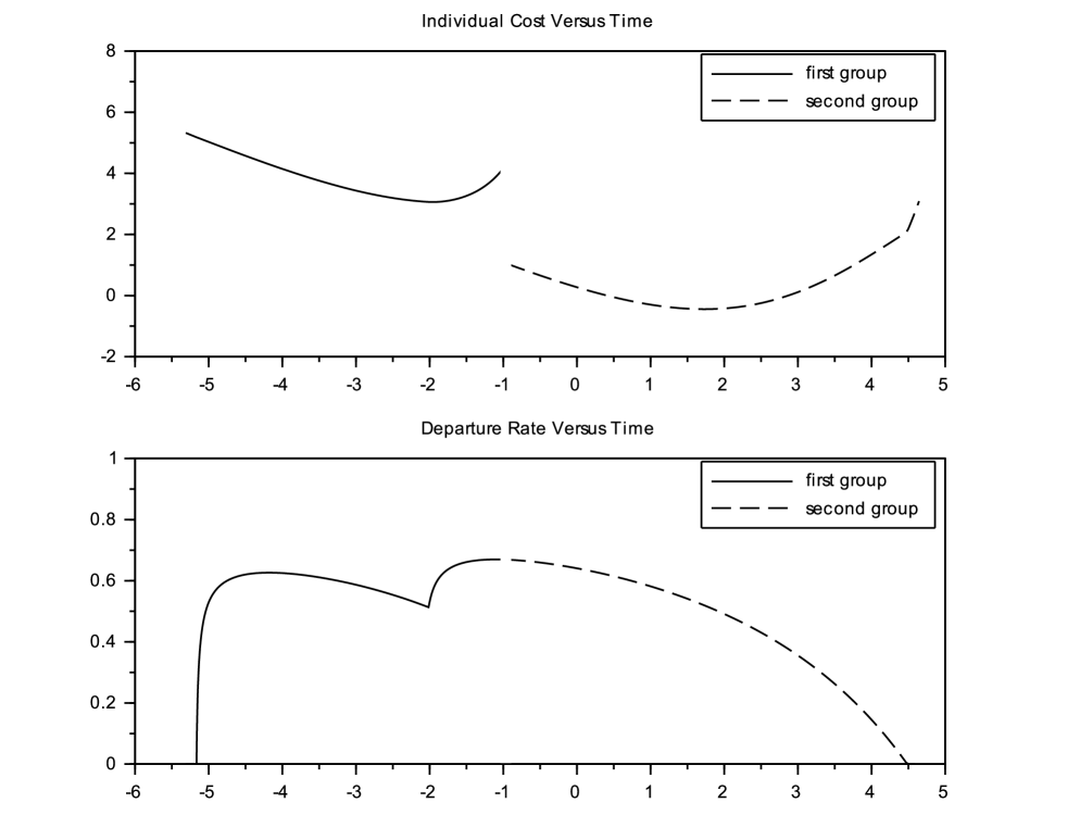
Example 4. We seek a globally optimal departure rate for two groups of drivers, with sizes $G_{1}=G_{2}=2.51$ on a road with length $L=10$. The conservation law governing traffic density is

$$\rho_{t}+[\rho v(\rho)]_{x}~{}=~{}0,\qquad v(\rho)\,=\,2-\rho$$ (5.7)

The departure and arrival costs for drivers of the two groups are

$$\varphi(t)~{}=~{}-t\qquad\psi_{1}(t)~{}=~{}e^{t-4}\qquad\psi_{2}(t)~{}=~{}e^{t-7.6}.$$ (5.8)

The optimal solution, found by the algorithm described above, is shown in Fig. 16. The marginal costs for adding one more driver of the first group or of the second group are found to be $\widehat{C}_{1}=5.18$ and $\widehat{C}_{2}=2.10$, respectively. Acknowledgment. This research was partially supported by NSF, with grant DMS-1411786: “Hyperbolic Conservation Laws and Applications”.

References

- [1] N. Bellomo, M. Delitala, and V. Coscia, On the mathematical theory of vehicular traffic flow. I. Fluid dynamic and kinetic modeling. Math. Models Methods Appl. Sci. 12 (2002), 1801-1843.
- [2] N. Bellomo and C. Dogbe, On the modeling of traffic and crowds: a survey of models, speculations, and perspectives. SIAM Review 53 (2011), 409–463.
- [3] A. Bressan, Hyperbolic Systems of Conservation Laws. The One Dimensional Cauchy Problem, Oxford University Press, 2000.
- [4] A. Bressan, S. Canic, M. Garavello, M. Herty, and B. Piccoli, Flow on networks: recent results and perspectives, EMS Surv. Math. Sci. 1 (2014), 47–111.
- [5] A. Bressan and K. Han, Optima and equilibria for a model of traffic flow. SIAM J. Math. Anal. 43 (2011), 2384–2417.
- [6] A. Bressan and K. Han, Nash equilibria for a model of traffic flow with several groups of drivers, ESAIM; Control, Optim. Calc. Var., 18 (2012), 969–986.
- [7] A. Bressan, C. J. Liu, W. Shen, and F. Yu, Variational analysis of Nash equilibria for a model of traffic flow, Quarterly Appl. Math. 70 (2012), 495–515.
- [8] A. Bressan and A. Marson, A variational calculus for discontinuous solutions of conservative systems, Comm. Part. Diff. Equat. 20 (1995), 1491–1552.
- [9] A. Bressan and A. Marson, A maximum principle for optimally controlled systems of conservation laws, Rend. Sem. Mat. Univ. Padova 94 (1995), 79–94.
- [10] A. Bressan and K. Nguyen, Conservation law models for traffic flow on a network of roads. Netw. Heter. Media 10 (2015), 255–293.
- [11] A. Bressan and K. Nguyen,Optima and equilibria for traffic flow on networks with backward propagating queues. Netw. Heter. Media 10 (2015), 717–748.
- [12] A. Bressan and A. Nordli, The Riemann Solver for traffic flow at an intersection with buffer of vanishing size. Netw. Heter. Media 12 (2017), 173–189.
- [13] A. Bressan and W. Shen, Optimality conditions for solutions to hyperbolic balance laws, in “Control Methods in PDE - Dynamical Systems”, F. Ancona, I. Lasieka, W. Littman, and R. Triggiani eds., AMS Contemporary Mathematics 426 (2007), 129–152.
- [14] A. Bressan and F. Yu, Continuous Riemann solvers for traffic flow at a junction. Discr. Cont. Dyn. Syst. 35 (2015), 4149–4171.
- [15] G. M. Coclite, M. Garavello, and B. Piccoli, Traffic flow on a road network. SIAM J. Math. Anal. 36 (2005), 1862–1886.
- [16] C. Dafermos, Polygonal approximations of solutions of the initial value problem for a conservation law, J. Math. Anal. Appl. 38 (1972), 33-41.
- [17] C. Daganzo, Fundamentals of Transportation and Traffic Operations, Pergamon-Elsevier, Oxford, U.K. (1997).
- [18] L. C. Evans, Partial Differential Equations. Second edition. American Mathematical Society, Providence, RI, 2010.
- [19] M. Garavello, K. Han, and B. Piccoli, Models for Vehicular Traffic on Networks, AIMS Series on Applied Mathematics, Springfield, Mo., 2016.
- [20] M. Garavello and B. Piccoli, Traffic Flow on Networks. Conservation Laws Models. AIMS Series on Applied Mathematics, Springfield, Mo., 2006.
- [21] M. Garavello and B. Piccoli, Traffic flow on complex networks. Ann. Inst. H. Poincaré, Anal. Nonlin. 26 (2009), 1925–1951.
- [22] M. Herty, S. Moutari, and M.Rascle, Optimization criteria for modeling intersections of vehicular traffic flow, Netw. Heterog. Media 1 (2006), 275–294.
- [23] H. Holden and N. H. Risebro. A mathematical model of traffic flow on a network of unidirectional roads. SIAM J. Math. Anal. 26 (1995), 999–1017.
- [24] P. D. Lax, Hyperbolic systems of conservation laws, Comm. Pure Appl. Math. 10 (1957), 537–556.
- [25] M. Lighthill and G. Whitham, On kinematic waves. II. A theory of traffic flow on long crowded roads. Proceedings of the Royal Society of London: Series A, 229 (1955), 317–345.
- [26] S. Pfaff and S. Ulbrich, Optimal boundary control of nonlinear hyperbolic conservation laws with switched boundary data. SIAM J. Control Optim. 53 (2015), 1250–1277.
- [27] P. I. Richards, Shock waves on the highway, Oper. Res. 4 (1956), 42-51.
- [28] J. Smoller, Shock waves and reaction-diffusion equations. Second edition. Springer-Verlag, New York, 1994.
- [29] S. Ulbrich, A sensitivity and adjoint calculus for discontinuous solutions of hyperbolic conservation laws with source terms. SIAM J. Control Optim. 41 (2002), 740–797.