Non-symmetric flexural wave scattering and one-way extreme absorption

Abstract

The possibility of asymmetric absorption and reflection for flexural waves is demonstrated though analytical and numerical examples. We focus on the 1D case of flexural motion of a beam and consider combinations of point scatterers which together provide asymmetric scattering. The scatterers are attached damped oscillators characterized by effective impedances, analogous to effective configurations in 1D acoustic waveguides. By selecting the impedances of a pair of closely spaced scatterers we show that it is possible to obtain almost total absorption for incidence on one side, with almost total reflection if incident from the other side. The one-way absorption is illustrated through numerous examples of impedance pairs that satisfy the necessary conditions for zero reflectivity for incidence from one direction. Examples of almost total and zero reflection for different incidences are examined in detail, showing the distinct wave dynamics of flexural waves as compared with acoustics.

I Introduction

An isolated lumped element in an acoustic waveguides produces symmetric reflection for sound incident from either side. This is true for standard sub-wavelength scatterers such as a side-branch Helmholtz resonator or a membrane stretched across the width of the waveguide. However, by combining elements, e.g. a Helmholtz resonator (HR) and a membrane in series, one can achieve asymmetric reflection depending on the direction of incidence. Such a combination of two or more point scatterers in a subwavelength configuration can be viewed as a new type of lumped element, called a Willis element Muhlestein2017a . Unlike the classical point scatterers the Willis element couples monopole and dipole radiation which in turn leads to asymmetry in the scattering, while it can still be viewed as a sub-wavelength point scatterer. The effective Willis parameters can be deduced from the scattering matrix elements Su2018a . An interesting case of asymmetric reflection is unidirectional zero reflection Merkel2018 in which the reflection is zero for incidence from one direction but non-zero from the other. The extreme limit of this phenomenon is one way total absorption where unidirectional zero reflection is accompanied by zero transmission. The transmission must therefore be zero for incidence from both directions, as required by acoustical reciprocity. However, while total asymmetric acoustic absorption implies zero symmetric transmission, the reflection coefficients can differ as much as zero and unity in magnitude. To the authors’ knowledge, this extreme limit of one way total absorption has not yet been demonstrated for the simplest setup: 1D waveguides.

The purpose of this paper is to show that one way total absorption can be obtained for flexural waves. Our analytical and numerical model is a 1D system of flexural wave motion in a beam, for which, by analogy with the lumped elements in an acoustic waveguide, we consider closely spaced translational point impedances. These may be modeled as attached single degree of freedom damped oscillators which apply an effective point force to the beam at the attachment point. We do not consider rotational impedance elements which can apply a moment Mead82 . Through proper choice of the complex impedances, we demonstrate that two attached damped oscillators display the same quantitative wave effects as acoustic one way total absorption. Specifically, reflection is zero for incidence from one side, while the reflection coefficient can be large, approaching unity in some cases, for waves incident from the opposite direction.

The present problem is related to but fundamentally differs from the control of flexural waves in a beam using a passive tuned vibration absorber (TVA) Brennan1997 ; Brennan1999 ; El-Khatib2005 . A TVA, modeled as a point translational impedance, can be used to minimize transmission or to reduce the vibration at a specific frequency for a source that is either in the farfield Brennan1999 or the near-field El-Khatib2005 . The term vibration neutralizer Brennan1997 rather than vibration absorber is sometimes used to signify that the purpose of the point attachment is to control vibration at a particular frequency.

Unlike a single TVA which necessarily has symmetric scattering properties for incidence from the left or the right, we consider two nearby impedances with the objective of maximizing the scattering asymmetry to obtain flexural wave one-way total absorption. The design objective is quite distinct from that of the TVA in that we wish to make one reflection zero and other as close to unity as possible. Here we are only concerned with passive wave control. We note that the reflection/transmission from two identical impedances was considered by Yang2016 where the effect of the spacing between the oscillators was found to be significant. However, the symmetric configuration gives the same reflection independent of the direction of incidence.

The outline of the paper is as follows. In Section II the governing equations are introduced and the solution is derived for scattering from two point impedances. Necessary and sufficient conditions for one of the reflection coefficients to vanish are derived in Section III. It is shown that asymmetric reflection requires at least one of the oscillators must be damped. In Section IV we show through numerous examples that one-way flexural reflection can be achieved from a wide variety of impedance pairs. For instance, one may be purely real (undamped) and the other imaginary (a pure damper), or both may be damped. We find, surprisingly, that it is possible to achieve almost perfect one-way reflection (zero one way, unity the other). This effect is explored in detail using asymptotic analysis in Section V. Finally, it is shown in Section VI that almost perfect one way reflection is achievable with a unique pair of impedances in the frequency range $ka\approx(\pi,2\pi)$. The main results are summarized and conclusions are presented in Section VII.

II Scattering by a cluster of point attachments

II.1 General solution

The beam has bending stiffness $D$ $(=EI)$ and density $\rho^{\prime}$ per unit length. Time harmonic motion $e^{-\mathrm{i}\omega t}$ is assumed, so that the flexural wavenumber $k$ is defined by $k^{4}=\omega^{2}\rho^{\prime}/D$. We assume there are $N$ point scatterers located at $x_{\alpha}$ with impedances $\mu_{\alpha}$, $\alpha=1,2,\ldots,N$. The total displacement $w$ satisfies

$$D\big{(}\frac{\operatorname{d}^{4}w(x)}{\operatorname{d}x^{4}}-k^{4}w\big{)}=\sum_{\alpha=1}^{N}\mu_{\alpha}w(x_{\alpha})\delta(x-x_{\alpha}).$$ (1)

The attachment impedance $\mu$ is modeled as single degree of freedom with mass $M$, spring stiffness $\kappa$ and damping coefficient $\nu$, and defined as $\mu=f/w$, where $f$ denotes the driving force. The impedance as used here is analogous to that for acoustics (pressure/velocity) although the two are not dimensionally equivalent. Two possible configurations are

$$\mu=\begin{cases}\big{(}\frac{1}{M\omega^{2}}-\frac{1}{\kappa-\mathrm{i}\omega\nu}\big{)}^{-1},&(a),\\ M\omega^{2}-\kappa+\mathrm{i}\omega\nu,&(b).\end{cases}$$ (2)

In case (a) the mass is attached to the plate by a spring and damper in parallel Torrent2013 , also called a vibration neutralizer Brennan1999 . Model (b) assumes the mass is rigidly attached to the plate, and both are attached to a rigid foundation by the spring and damper in parallel Evans2007 . An important limit is a beam pinned at $x_{\alpha}$, $w(x_{\alpha})=0$, which corresponds to $\mu\to\infty$. The (a) and (b) oscillators could also be attached in parallel, e.g. on either side of the beam, to give $\mu=\mu_{a}+\mu_{b}$. The main point is that there is a wide range of achievable passive $\mu$ $(\operatorname{Im}\mu\geq 0)$. We take advantage of this adaptivity by exploring the space of possible impedances in this paper.

The solution is given by the incident wave $w_{\text{in}}(x)$ plus the displacement scattered by all the particles,

$$w(x)=w_{\text{in}}(x)+\sum_{\beta=1}^{N}G(x-x_{\beta})\mu_{\beta}w(x_{\beta})$$ (3)

where the Green’s function satisfies

$$D\big{(}\frac{\operatorname{d}^{4}G(x)}{\operatorname{d}x^{4}}-k^{4}G(x)\big{)}=\delta(x).$$ (4)

We choose to normalize parameters so that the impedances and the Green’s function are nondimensional. Define

$$m_{\alpha} =\frac{2Dk^{3}}{\mu_{\alpha}},$$ (5a)

$$g(x) =2Dk^{3}G(x)=\frac{\mathrm{i}}{2}\big{(}e^{\mathrm{i}k|x|}+\mathrm{i}e^{-k|x|}\big{)},$$ (5b)

then (3) becomes

$$w(x)=w_{\text{in}}(x)+\sum_{\beta=1}^{N}g(x-x_{\beta})m_{\beta}^{-1}w(x_{\beta}).$$ (6)

Setting $x=x_{\alpha}$ in (6) gives a linear system of $N$ equations which may be solved to give

$$w(x)=w_{\text{in}}(x)+\sum_{\alpha,\beta=1}^{N}g(x-x_{\alpha})M_{\alpha\beta}^{-1}\,w_{\text{in}}(x_{\beta})$$ (7)

where $M_{\alpha\beta}^{-1}$ are the elements of the inverse of the $N\times N$ matrix with elements

$$M_{\alpha\beta}=m_{\alpha}\delta_{\alpha\beta}-g(x_{\alpha}-x_{\beta}).$$ (8)

II.2 Reflection, transmission and absorption coefficients

We consider incidence from the left and right, $w_{\text{in}}^{+}$ and $w_{\text{in}}^{-}$, respectively,

$$w_{\text{in}}^{\pm}(x)=e^{\pm\mathrm{i}kx}.$$ (9)

The reflection coefficients $R_{+}$, $R_{-}$ and the single transmission coefficient $T$ are defined by

$$w(x) =\begin{cases}w_{\text{in}}^{+}+R_{+}e^{-\mathrm{i}kx},&x\to-\infty,\\ w_{\text{in}}^{-}+R_{-}e^{\mathrm{i}kx},&x\to\infty,\end{cases}$$ (10a)

$$w(x) =Te^{\pm\mathrm{i}kx},\ \ x\to\pm\infty\ \text{for }\ w_{\text{in}}^{\pm}.$$ (10b)

These follow from (7) as

$$R_{\pm} =\frac{\mathrm{i}}{2}\sum_{\alpha,\beta=1}^{N}M_{\alpha\beta}^{-1}\,e^{\pm\mathrm{i}k(x_{\alpha}+x_{\beta})},$$ (11a)

$$T =1+\frac{\mathrm{i}}{2}\sum_{\alpha,\beta=1}^{N}M_{\alpha\beta}^{-1}\,e^{\mathrm{i}k(x_{\alpha}-x_{\beta})}.$$ (11b)

To quantify absorption, we define absorption coefficients for right and left incidence $\alpha^{+}$ and $\alpha^{-}$, respectively, as

$$\alpha^{\pm}=1-|T|^{2}-|R_{\pm}|^{2}.$$ (12)

II.3 Example: One and two scatterers

It is useful to recall some of the features of a single translational impedance before we consider two attachments.

II.3.1 One scatterer

For a single scatterer at $x=0$ we have $R_{\pm}=R=\frac{\mathrm{i}}{2}(m-g(0))^{-1}$ and $T=1+R$. A desired value of $T$ (or $R=T-1$) is obtained if

$$m=-\frac{1}{2}+\frac{\mathrm{i}T}{2(T-1)}\ \ \Rightarrow\ \ w(0)=-\mathrm{i}+(1+\mathrm{i})T.$$ (13)

Thus, for instance, $w(0)=0$ for $m=0$ (infinite impedance $\mu$). Even though the beam is pinned the rotation at $x=0$ is not constrained, and hence half of the incident energy is transmitted and half is reflected: $|R|=|T|=1/\sqrt{2}$. Zero transmission ($T=0$) is obtained if $m=-\frac{1}{2}$, which is interpreted in terms of model (a) of Eq. (2) by Brennan1999 ; El-Khatib2005 : the unique frequency at which $T$ vanishes is given by (Brennan1999, , Eq. (7)) or (El-Khatib2005, , Eq. (22)). In general, the range of possible values of $T$ for the single scatterer is restricted only by the requirement that the attachment is passive, i.e. $\operatorname{Im}m\leq 0$ $\Leftrightarrow$ $\operatorname{Re}T\geq|T|^{2}\leq 1$.

The full transmission or - equivalently - the zero reflection case, namely $|T|\rightarrow 1\Leftrightarrow|R|\rightarrow 0$, from (13) corresponds to $m\rightarrow\infty\Leftrightarrow\mu\rightarrow 0$, so no scatterer. Also $w(x=0)=e^{\mathrm{i}kx}\vline_{x=0}=1$ as given by (13) with $T=1$.

II.3.2 Two scatterers

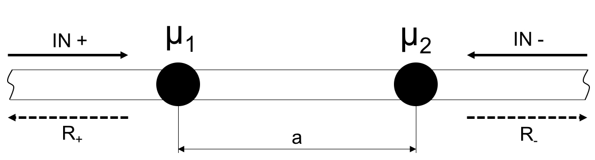
Figure 1: Schematic of the $N=2$ system.

For $N=2$, let $x_{1}=-\frac{a}{2}$, $x_{2}=\frac{a}{2}$; a schematic of the system is shown in figure 1. The matrix ${\bf M}$ is

$${\bf M}=\begin{pmatrix}m_{1}-g(0)&-g(a)\\ -g(a)&m_{2}-g(0)\end{pmatrix}$$ (14)

implying

$$R_{\pm} =\frac{\mathrm{i}}{2\det{\bf M}}\Big{(}m_{1}e^{\pm\mathrm{i}ka}+m_{2}e^{\mp\mathrm{i}ka}-{2g(0)\cos ka+2g(a)}\Big{)},$$ (15a)

$$T =1+\frac{\mathrm{i}}{2\det{\bf M}}\big{(}m_{1}+m_{2}-2g(0)+2g(a)\cos ka\big{)}.$$ (15b)

The reflection coefficients can be written

$$R_{\pm}= \frac{g^{2}(0)}{\det{\bf M}}\Big{(}e^{-ka}+\sin ka-\cos ka-(m_{1}+m_{2})\cos ka$$

$$\pm\mathrm{i}(m_{2}-m_{1})\sin ka\big{)}\Big{)}.$$ (16)

This form shows that $|R_{+}|=|R_{-}|$ if $\mu_{1}$ and $\mu_{2}$ are real. In that case there is no damping and the energy identity is satisfied:

$$|R_{\pm}|^{2}+|T|^{2}=1\ \ \text{for real }\mu_{1},\ \mu_{2}.$$ (17)

The reflection coefficients can vanish, for instance, if $ka=\pi$ and $m_{1}+m_{2}+1+e^{-\pi}=0$, or if $m_{1}=m_{2}=\frac{1}{2}\big{(}\tan ka+e^{-ka}\sec ka-1\big{)}$.

When the separation $a\to 0$, Equation (II.3.2) yields $R_{+}=R_{-}$ with the two attachments acting as a single one with impedance $\mu=\mu_{1}+\mu_{2}$.

III One way zero reflection: impedance conditions

We are interested in configurations in which one of the reflection coefficients vanishes but the other remains finite. As shown above, the magnitudes of the reflection coefficients coincide for real-valued impedances. Therefore, in order to have $|R_{+}|\neq|R_{-}|$ requires that at least one of the impedances $\mu_{1},\ \mu_{2}$ is complex valued. We assume they are passive dampers, which means that $\operatorname{Im}m_{\alpha}\leq 0$ for both $\alpha=1$ and $2$. Assume $R_{+}=0$, then

$$R_{-}=\frac{(m_{1}-m_{2})}{\det{\bf M}}\sin ka$$ (18)

subject to the constraint implied by $R_{+}=0$,

$$e^{-ka}+\sin ka-\cos ka-(m_{1}+m_{2})\cos ka+\mathrm{i}(m_{2}-m_{1})\sin ka=0.$$ (19)

Equivalently,

$$m_{+}\cot ka+\mathrm{i}m_{-}=K$$ (20)

where $m_{+}$, $m_{-}$ and $K=2\big{(}g(0)\cos ka-g(a)\big{)}/\sin ka$ are

$$m_{\pm} =m_{1}\pm m_{2},$$ (21)

$$K =1-\cot ka+e^{-ka}/\sin ka.$$ (22)

Viewing $m_{+}$ as the determining parameter, we have $R_{+}=0$ and

$$m_{1} =\frac{m_{+}}{2}+\frac{\mathrm{i}}{2}(m_{+}\cot ka-K),$$ (23a)

$$m_{2} =\frac{m_{+}}{2}-\frac{\mathrm{i}}{2}(m_{+}\cot ka-K),$$ (23b)

$$R_{-} =2\mathrm{i}\sin^{2}ka\frac{\big{(}[\frac{1}{2}m_{+}-g(0)]\cos ka+g(a)\big{)}}{\big{(}\frac{1}{2}m_{+}-g(0)+g(a)\cos ka\big{)}^{2}},$$ (23c)

$$T =1+\frac{\mathrm{i}\sin^{2}ka}{\frac{1}{2}m_{+}-g(0)+g(a)\cos ka}.$$ (23d)

One reason for considering $m_{+}$ to be the control parameter is that, unlike $m_{-}$, it must lie in the negative half of the complex plane, $\operatorname{Im}m_{+}\leq 0$. This does not, however, guarantee that both $m_{1}$ and $m_{2}$ are in the same half plane. Therefore the choice of $m_{+}$ must be restricted by the passivity requirements $\operatorname{Im}m_{\alpha}\leq 0$, $\alpha=1,2$. The case $\operatorname{Im}m_{+}=0$ is of no interest, and we therefore concentrate on $\operatorname{Im}m_{+}<0$.

Define

$$m=m^{\prime}+\mathrm{i}m^{\prime\prime}$$ (24)

then the reflection coefficient $R_{+}$ vanishes if

$$m_{+}^{\prime}\cot ka-m_{-}^{\prime\prime} =K,$$ (25a)

$$m_{+}^{\prime\prime}\cot ka+m_{-}^{\prime} =0,$$ (25b)

where $ka\in(0,\pi)$. The non-zero reflection coefficient $R_{-}$ of (18) can be rewritten as

$$R_{-}=\frac{-m^{\prime\prime}_{+}\cos ka+\mathrm{i}m^{\prime\prime}_{-}\sin ka}{\det{\bf M}},$$ (26)

indicating that damping is essential in order to have $R_{-}\neq 0$.

Of interest is therefore the part of the parameter space, $(m^{\prime\prime}_{+},m^{\prime\prime}_{-})$ or - equivalently - $(m^{\prime\prime}_{1},m^{\prime\prime}_{2})$, where at least one of the scatterers displays passive damping properties, i.e. $m^{\prime\prime}_{\alpha}<0$. Each point in this space uniquely defines the pair of scatterers in terms of their damping properties, but not their mass-stiffness properties or the spacing $a$ between them. Figure 2 illustrates this space with the shaded area corresponding to the desired passive damping properties of the scatterers. It can be noted that $(m^{\prime\prime}_{+},m^{\prime\prime}_{-})$ and $(m^{\prime\prime}_{1},m^{\prime\prime}_{2})$ coordinate systems are related by a $\pi/4$ rotation and $\sqrt{2}$ stretch through the transformation given in (21). Passivity conditions, analogous to $m_{1}^{\prime\prime}<0$ and $m_{2}^{\prime\prime}<0$, are therefore given as $|m_{-}^{\prime\prime}|<-m_{+}^{\prime\prime}$.

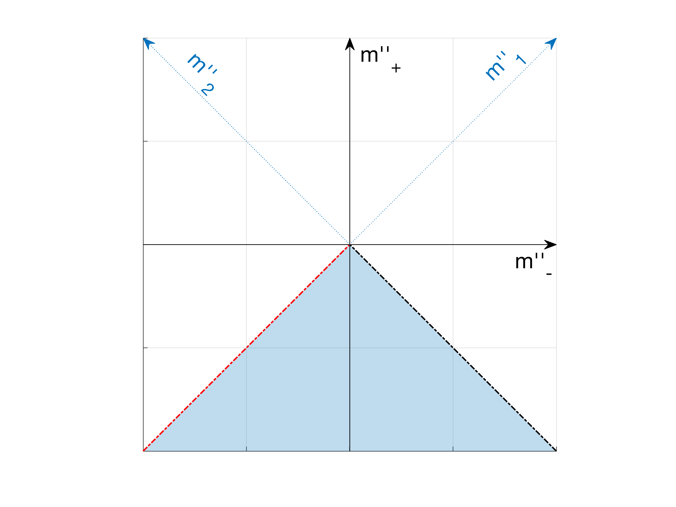
Figure 2: Design space for the two-scatterer case defined in terms of $(m^{\prime\prime}_{+},m^{\prime\prime}_{-})$ or $(m^{\prime\prime}_{1},m^{\prime\prime}_{2})$. The shaded area marks all negative imaginary parts of $m_{\alpha}$ of the two scatterers, corresponding to passive damping properties.

IV Examples of one way reflection

It was shown in section III that damping is critical to obtain one way zero reflection. We will therefore consider the pair of scatterers $(\alpha,\beta)$ described by two complex normalized impedances $m_{\alpha,\beta}=m_{\alpha,\beta}^{\prime}+\mathrm{i}m_{\alpha,\beta}^{\prime\prime}$ with passive damping properties ($m_{\alpha,\beta}^{\prime\prime}<0$).

We start by investigating a setup composed of two scatterers where one is described by purely real $m_{\alpha}=m_{\alpha}^{\prime}$, while the other by a complex normalized impedance $m_{\beta}=m_{\beta}^{\prime}+\mathrm{i}m_{\beta}^{\prime\prime}$, with $m_{\beta}^{\prime\prime}<0$. As the system is non-reciprocal, its response is non-symmetric with respect to the selection of $\alpha$ and $\beta$, namely for $(\alpha,\beta)=(1,2)$ and $(\alpha,\beta)=(2,1)$. We will therefore distinguish the two cases.

Next, we consider cases of two scatterers with passive damping properties, i.e. $m_{\alpha,\beta}^{\prime\prime}<0$. Starting with the case of the same negative normalized impedance $m_{\alpha}^{\prime\prime}=m_{\beta}^{\prime\prime}=m^{\prime\prime}<0$, we then generalize to $m_{\alpha}^{\prime\prime}\neq m_{\beta}^{\prime\prime}<0$ and relate this general case to results obtained for other configurations of the scatterers.

IV.1 First impedance purely real: $m_{1}^{\prime\prime}=0$

When $(\alpha,\beta)=(1,2)$, we have $m_{1}=m_{1}^{\prime}$, $(m_{1}^{\prime\prime}=0)$ and $m_{2}=m_{2}^{\prime}+\mathrm{i}m_{2}^{\prime\prime}$, with $m_{2}^{\prime\prime}<0$, i.e. we investigate scatterer configurations along an edge of the passive zone (see the black dash-dot line in figure 2). Then, $m_{+}^{\prime\prime}=m_{2}^{\prime\prime}$ and $m_{-}^{\prime\prime}=-m_{2}^{\prime\prime}$ and the relation between $m_{+}^{\prime}$ and $m_{-}^{\prime}$ follows from (25) as

$$\big{(}m_{+}^{\prime}\cot ka-K\big{)}\cot ka-m_{-}^{\prime}=0,\ \ \ \ \ \ \ \ m_{2}^{\prime\prime}=m_{+}^{\prime\prime}=-m_{-}^{\prime\prime}<0.$$ (27)

From equations (25) and (27) we also have that

$$m_{-}^{\prime}\gtrless 0,\ \ m_{+}^{\prime}\cot ka\gtrless K,\ \ \text{for}\ \ \left\{\begin{matrix}k\in(0,\pi/2),\\ k\in(\pi/2,\pi).\end{matrix}\right.$$ (28)

Equation (27) with constraints in (28) define a surface in $(m_{+}^{\prime},m_{-}^{\prime})$ space that is illustrated in figure 3. Relation (27) can be mapped to $(m_{1}^{\prime},m_{2}^{\prime})$ coordinates through (21) to find corresponding real parts $m_{1}^{\prime}$ and $m_{2}^{\prime}$ of the complex impedances. Two particular configurations can be then obtained by cutting the design space from figure 3 with the $m_{1}^{\prime}=0$ or $m_{2}^{\prime}=0$ planes resulting in one of the impedances being purely real and the other purely imaginary.

IV.1.1 Second impedance purely imaginary.

Continuing with $(\alpha,\beta)=(1,2)$ (impedance $\mu_{1}$ is purely real), but specializing to the case of $\mu_{2}$ purely imaginary $(m_{1}^{\prime\prime}=m_{2}^{\prime}=0,\,m_{-}=\overline{m}_{+})$, corresponds to a particular solution of the family of solutions illustrated in figure 3 by red lines. Then (25) implies that

$$m_{1}^{\prime}=\frac{K\cot ka}{\cot^{2}ka-1},\ \ \ m_{2}^{\prime\prime}=\frac{-K}{\cot^{2}ka-1}.$$ (29)

Figure 4 shows the required values of $m_{1}^{\prime}$ and $m_{2}^{\prime\prime}$ and the corresponding reflection and transmission coefficients, $|R_{+}|$, $|R_{-}|$ and $|T|$. The impedance $\mu_{2}$ for this model is passive for $ka\in(0,\frac{\pi}{4})$ and $ka\in(\frac{3\pi}{4},\pi)$. Note that the intersection of the surface given by (27) with $m_{1}^{\prime}=0$ reduces to a point at $ka=0$.

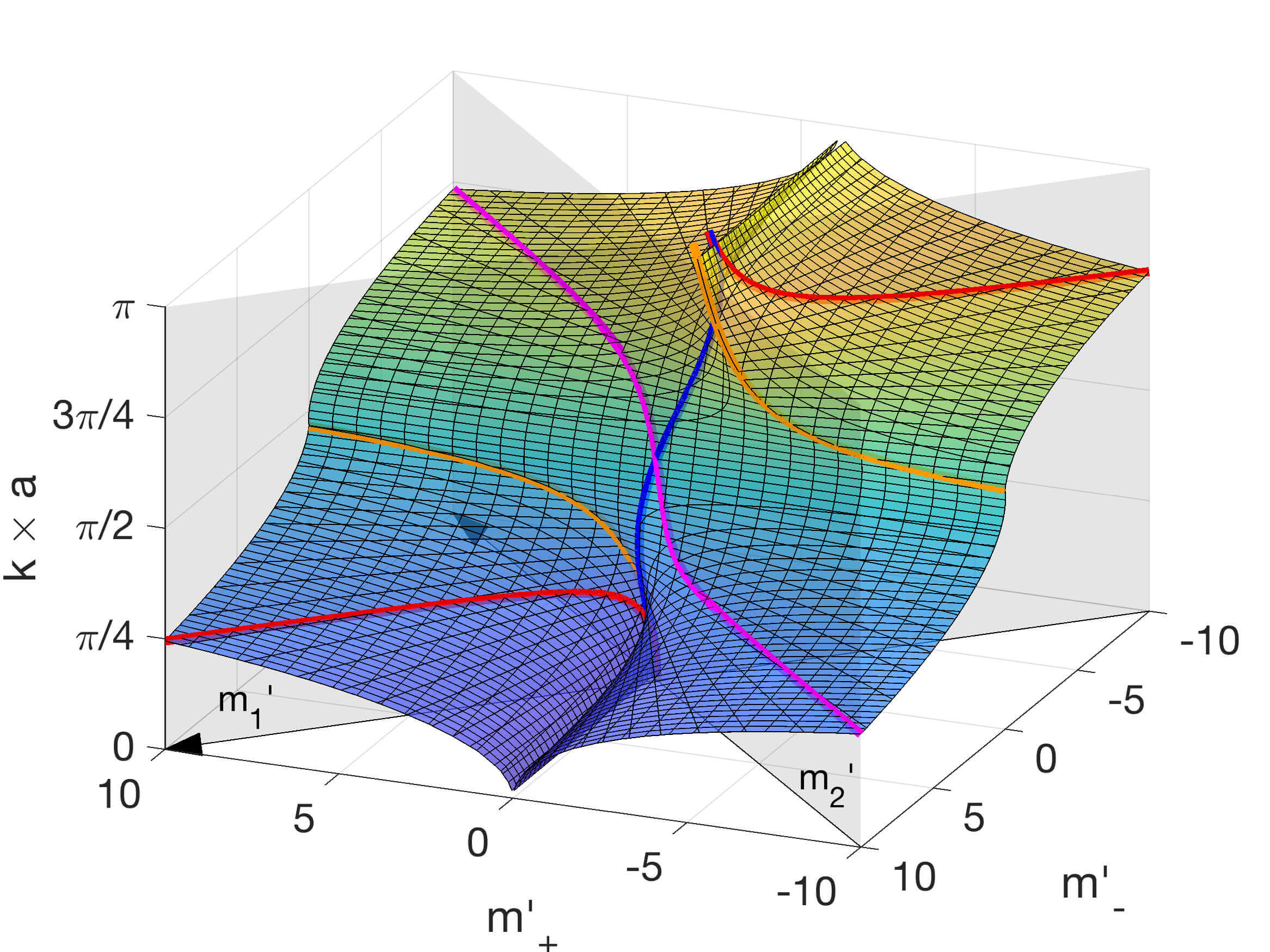
Figure 3: Design space, $|m_{-}^{\prime\prime}|<-m_{+}^{\prime\prime}$, corresponding to negative imaginary parts of $m_{1}$ and $m_{2}$ mapped through equations (25) (see figure 2). The color lines indicate special configurations of scatterers described in the text. Solutions for the red, magenta, blue and orange curves are given in figures 4, 5, 6 and 11, respectively.

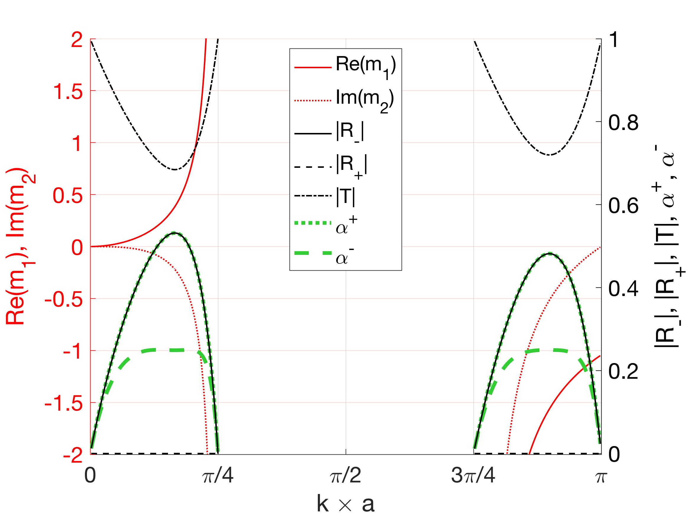
Figure 4: The normalized impedances for zero one-way reflection from equation (29). In this case $\mu_{1}$ is real and $\mu_{2}$ is positive imaginary and hence passive.

IV.2 Second impedance purely real: $m_{2}^{\prime\prime}=0$

If $(\alpha,\beta)=(2,1)$, then $m_{2}^{\prime\prime}=0$ ($m_{2}=m_{2}^{\prime}$) and $m_{1}=m_{1}^{\prime}+\mathrm{i}m_{1}^{\prime\prime}$ with $m_{1}^{\prime\prime}<0$ corresponding to the red dash-dot line in figure 2. In this case $m_{+}^{\prime\prime}=m_{1}^{\prime\prime}$ and $m_{-}^{\prime\prime}=m_{1}^{\prime\prime}$ and the relation between $m_{+}^{\prime}$ and $m_{-}^{\prime}$ yields

$$\big{(}m_{+}^{\prime}\cot ka-K\big{)}\cot ka+m_{-}^{\prime}=0,\ \ \ \ \ \ \ \ m_{1}^{\prime\prime}=m_{+}^{\prime\prime}=m_{-}^{\prime\prime}<0,$$ (30)

while equations (25) and (30) imply the constraints

$$m_{-}^{\prime}\gtrless 0,\ \ m_{+}^{\prime}\cot ka\lessgtr K,\ \ \text{for}\ \ \left\{\begin{matrix}k\in(0,\pi/2),\\ k\in(\pi/2,\pi).\end{matrix}\right.$$ (31)

The design space given by (30) is shown in figure 3. As before, two particular configurations can be seen by cutting the design space from figure 3 by the $m_{1}^{\prime}=0$ or $m_{2}^{\prime}=0$ planes, subject to the constraints (31).

IV.2.1 First impedance purely imaginary.

When mapping (30) on the $m_{2}^{\prime}$ plane, i.e. taking $m_{1}^{\prime}=0$, we have $m_{1}=\mathrm{i}m_{1}^{\prime\prime}$, $m_{1}^{\prime\prime}<0$ and $m_{2}=m_{2}^{\prime}$. The first impedance purely negative imaginary while the second is purely real $(m_{-}=-\overline{m}_{+})$, a situation opposite to that considered previously, with

$$m_{1}^{\prime\prime}=\frac{K}{\cot^{2}ka-1},\ \ \ m_{2}^{\prime}=\frac{K\cot ka}{\cot^{2}ka-1}.$$ (32)

Figure 5 shows the required values of $m_{1}^{\prime\prime}$ and $m_{2}^{\prime}$ and the corresponding reflection and transmission coefficients, $|R_{+}|$, $|R_{-}|$ and $|T|$.

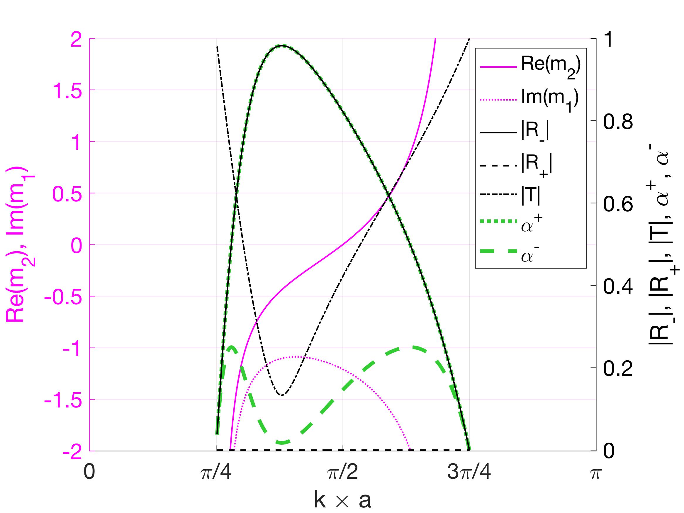
Figure 5: The normalized impedances for zero one-way reflection from equation (32). In this case $\mu_{2}$ is real and $\mu_{1}$ is positive imaginary and hence passive.

IV.2.2 Second impedance infinite (pinned point).

Due to asymmetry of the design space, another interesting scatterer configuration can be found by mapping (30) onto the $m_{1}^{\prime}$ plane. Then, $m_{2}^{\prime}=0$, making the second normalized impedance vanish and resulting in $\mu_{2}=\infty$, i.e. a pinned point. Note that from the definition of the impedance and the governing equation (1) it follows that energy can be transferred across a pinned point through rotations of the beam cross sections proportional to $\frac{dw}{dx}$ even if $w=0$. This particular feature distinguishes the flexural wave problem from the acoustic one. In this case the other normalized impedance, $m_{1}=m_{1}^{\prime}+\mathrm{i}m_{1}^{\prime\prime}$, is complex with

$$m_{1}^{\prime}=K\sin ka\cos ka,\ \ \ m_{1}^{\prime\prime}={-K}{\sin^{2}ka}.$$ (33)

Figure 6 shows the real and imaginary parts of the complex normalized impedance for the first scatterer. Interestingly, with the second point pinned, $m_{2}=0$, it is possible to obtain one-way reflection over wide wavenumber (or frequency) band.

Passive $ka$	$m_{1}^{\prime}$	$m_{1}^{\prime\prime}$	$m_{2}^{\prime}$	$m_{2}^{\prime\prime}$	Figure	Sec.
$(0,\frac{\pi}{4}),(\frac{3}{4}{\pi},\pi)$	$\frac{K}{2}\tan 2ka$	$0$	$0$	$-\frac{K}{2}\tan 2ka\tan ka$	4	IV.1.1
$(\frac{\pi}{4},\frac{3}{4}\pi)$	$0$	$\frac{K}{2}\tan 2ka\tan ka$	$\frac{K}{2}\tan 2ka$	$0$	5	IV.2.1
$(0,{\pi})$	$\frac{K}{2}\sin 2ka$	$-K\sin^{2}ka$	$0$	$0$	6	IV.2.2
$(0,{\pi})$	$\frac{K}{2}\tan ka-m^{\prime\prime}\cot ka$	$m^{\prime\prime}$	$\frac{K}{2}\tan ka+m^{\prime\prime}\cot ka$	$m^{\prime\prime}$	7,8,9	IV.3
$(0,{\pi})$	$K\tan ka$	$-\frac{K}{2}\tan^{2}ka$	$0$	$-\frac{K}{2}\tan^{2}ka$	10	IV.3.1
$(0,{\pi})$	$\frac{K}{2}\tan ka\pm\Delta_{-}^{(2)}$	$\mp\Delta^{(0)}_{+}\tan ka$	$\frac{K}{2}\tan ka\mp\Delta_{+}^{(2)}$	$\mp\Delta^{(0)}_{-}\tan ka$	11, 12	IV.4
${ka\ll 1\atop ka\approx\pi}$	$\frac{K}{2}\tan ka-m^{\prime\prime}\cot ka$	$m^{\prime\prime}\ll 1$	$\frac{K}{2}\tan ka+m^{\prime\prime}\cot ka$	$m^{\prime\prime}\ll 1$	14	${\ref{sec51}\atop\ref{sec52}}$
$\approx(\pi,2\pi)$	$m_{2}^{\prime}+\frac{1}{2}\sin 2ka$	$-m_{2}^{\prime\prime}-\sin^{2}ka$	$-\frac{1}{2}+\frac{1}{2}e^{-ka}\cos ka$	$\frac{1}{2}e^{-ka}\sin ka$		VI

Table 1: A summary of the special cases corresponding to the red, blue, magenta and orange curves in Figure 3, considered in this work. Note $m_{1}^{\prime\prime}\leq 0,m_{2}^{\prime\prime}\leq 0$, ensuring passive configurations and $\Delta^{(n)}_{\pm}=\frac{\delta}{2}\big{(}1\pm\frac{1}{c}{\tan^{n}ka}\big{)}$ for $n=0,2$.

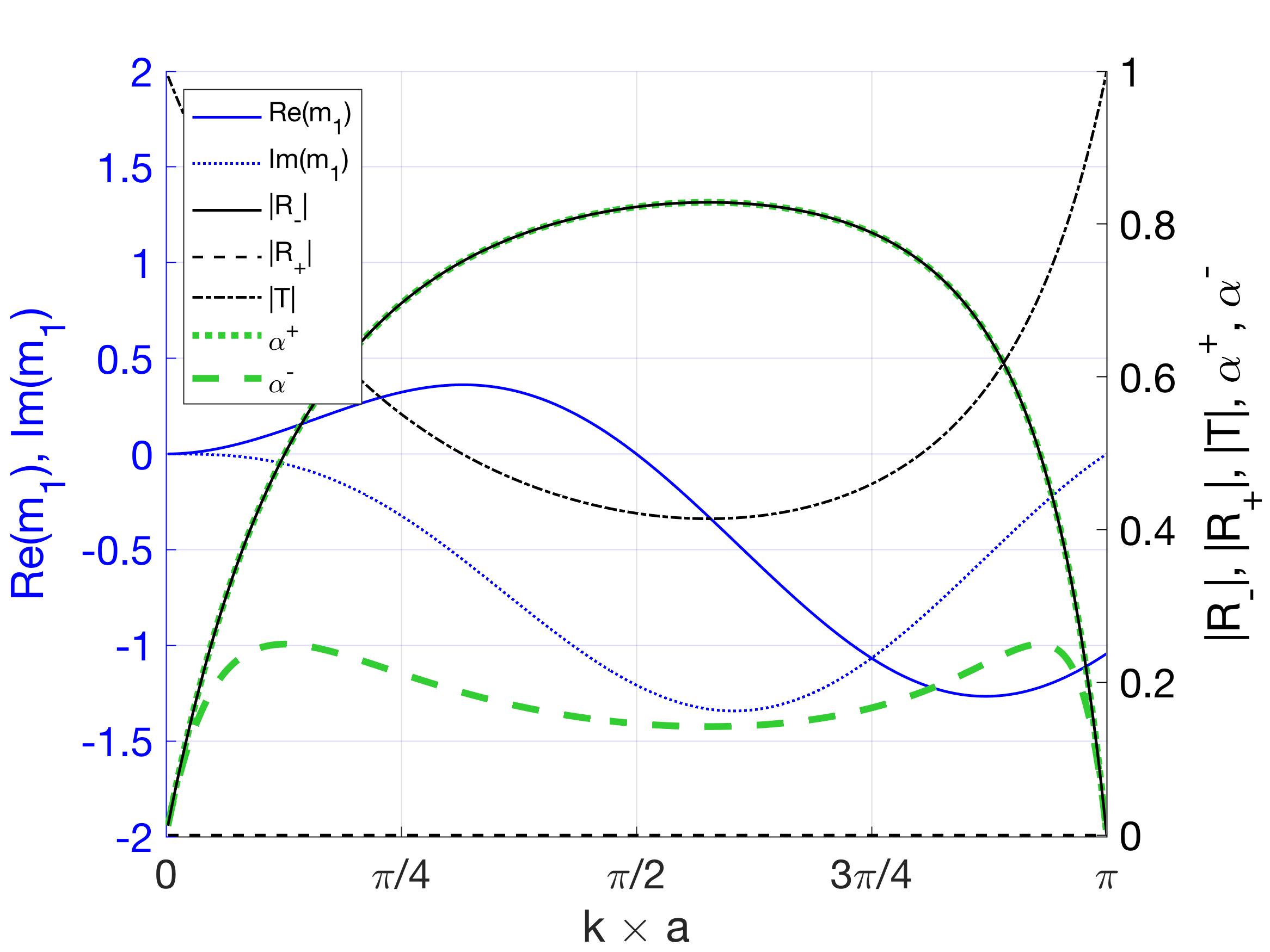
Figure 6: The normalized impedances for zero one-way reflection from equation (33), corresponding to the blue curve in figure 3. In this case $m_{2}=0$ ($\mu_{2}=\infty$) indicating a pinned point, and $m_{1}=m_{1}^{\prime}+\mathrm{i}m_{1}^{\prime\prime}$ is complex with $m_{1}^{\prime\prime}<0$ and hence passive.

IV.2.3 Second impedance infinite (pinned point) with a pure damper.

Note the exchanged positions (but the same values) of the real parts of normalized impedances shown in rows 2 and 3 of table 1. A particular selection of $k\times a=\pi/2$ results in the real parts of scatterers in rows 2 and 3 - $m^{\prime}_{2}$ and $m^{\prime}_{1}$, respectively - equal to zero. Therefore, for this specific configuration we have the second scatterer pinned ($\mu_{2}=\infty$) while the first is purely negative imaginary (passive damper). The imaginary parts of the normalized impedances $m^{\prime\prime}_{1}$ from (32) and (33) are both $m^{\prime\prime}_{1}=-K=-(1+e^{-\pi/2})<0$.

IV.3 Impedances with the same passive damping properties: $m_{1}^{\prime\prime}=m_{2}^{\prime\prime}$

Selecting passive damping properties other than discussed above, results in configurations with imaginary parts of normalized impedances being both nonzero. A particular choice is $m_{1}^{\prime\prime}=m_{2}^{\prime\prime}<0$ or, equivalently $m_{-}^{\prime\prime}=0$ and $m_{+}^{\prime\prime}<0$. With $m_{1}^{\prime\prime}=m_{2}^{\prime\prime}=m^{\prime\prime}<0$ equations (25) lead to

$$m_{+}=K\tan ka+\mathrm{i}2m^{\prime\prime}.$$ (34)

Therefore from (23), the two impedances are

$$m_{1} =\frac{1}{2}K\tan ka-m^{\prime\prime}\cot ka+\mathrm{i}m^{\prime\prime},$$ (35)

$$m_{2} =\frac{1}{2}K\tan ka+m^{\prime\prime}\cot ka+\mathrm{i}m^{\prime\prime},$$

implying $|m_{1}^{\prime}|>|m_{2}^{\prime}|$. It is therefore not possible to obtain one-way reflection with a pair of scatterers with the same negative imaginary part of the complex impedance having the same or opposite real parts (i.e. mass and stiffness properties). Equation (35) implies

$$(m_{1}^{\prime})^{2}-(m_{2}^{\prime})^{2}=-2m^{\prime\prime}K\ \ \Leftrightarrow\ \ m_{+}^{\prime}m_{-}^{\prime}=-2m^{\prime\prime}K$$ (36)

which defines a hyperbola in $(m_{1}^{\prime},m_{2}^{\prime})$ (or $(m_{+}^{\prime},m_{-}^{\prime})$) space for each selected value of $m^{\prime\prime}$, as shown in figure 7.

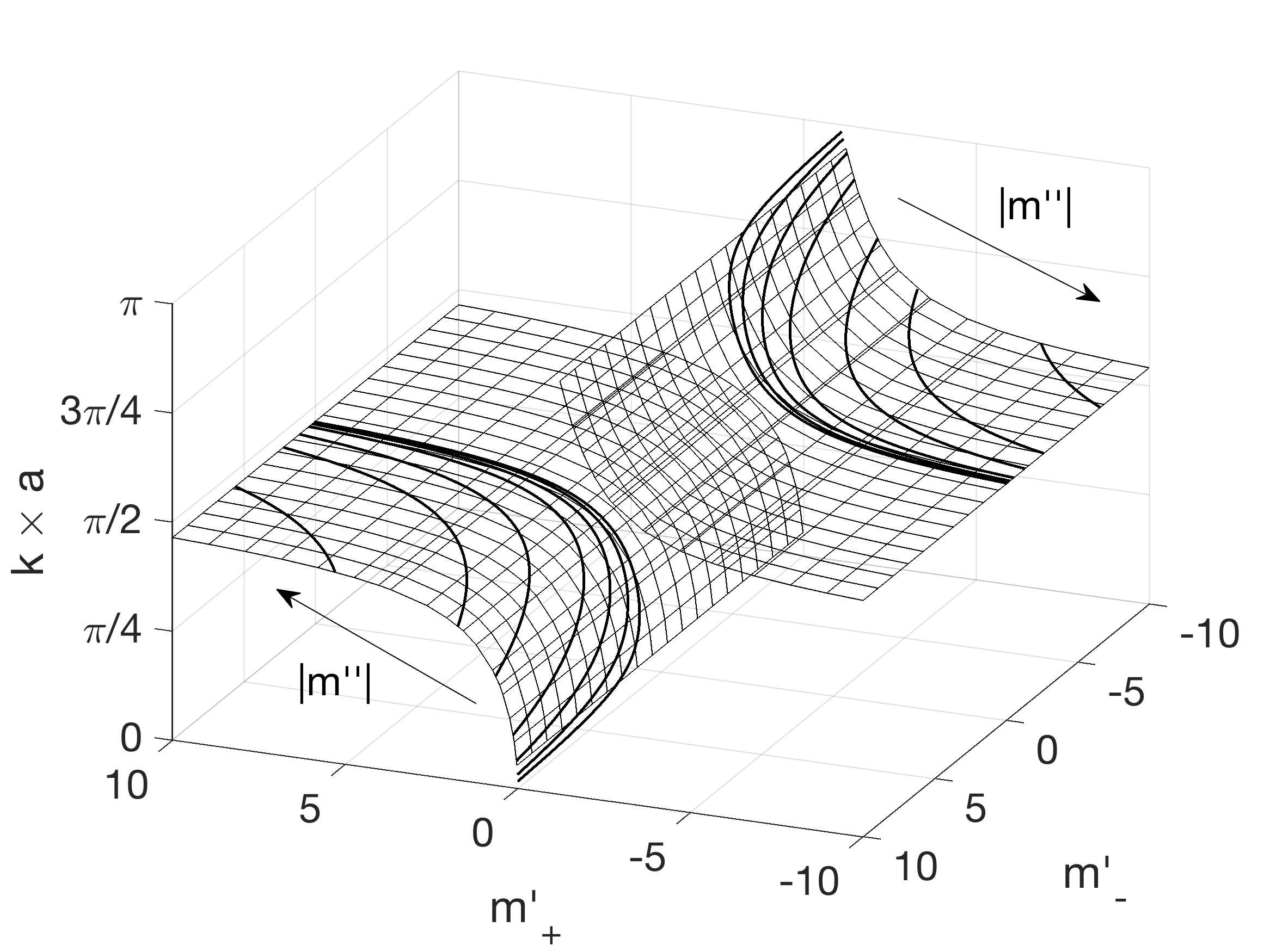
Figure 7: Examples of normalized impedance curves for various selected values of $m^{\prime\prime}<0$ for $m_{+}^{\prime\prime}<0$ and $m_{-}^{\prime\prime}=0$, based on Equation (35).

Values of $m_{1}^{\prime}$ and $m_{2}^{\prime}$ required for the one-way zero reflection with $|R_{+}|=0$ are shown in figure 8. The corresponding reflection $|R_{-}|$ and transmission $|T|$ coefficients are shown in figure 9. Note the possibility of obtaining narrow-band highly directional properties of the system when $m^{\prime\prime}\rightarrow 0$ and $k\times a\rightarrow 0$ or $k\times a\rightarrow\pi$. Those special cases are discussed in detail later.

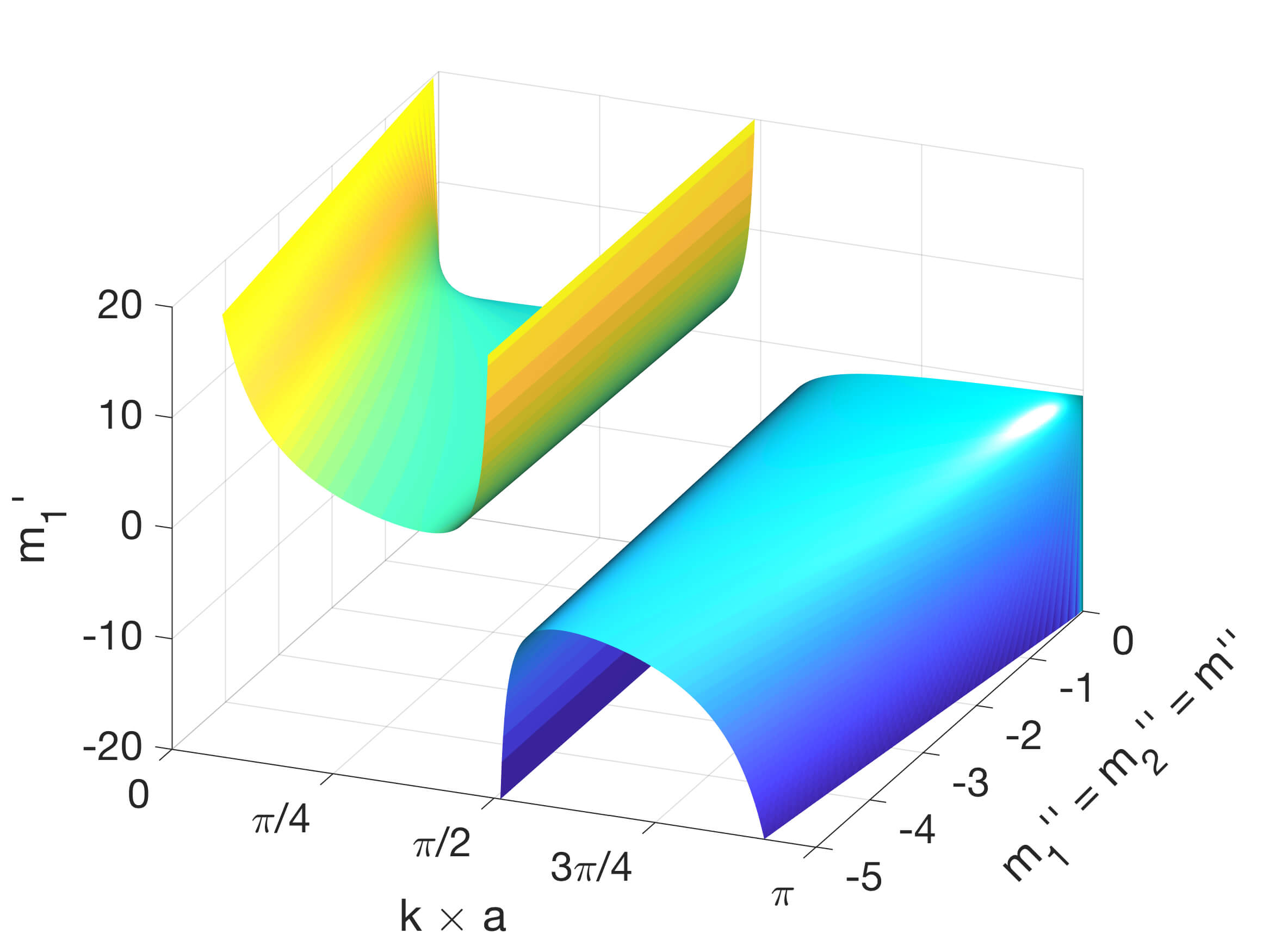
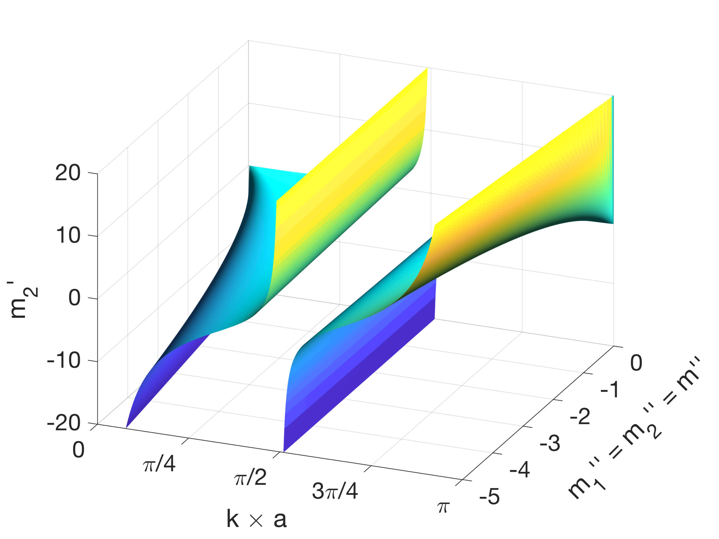
Figure 8: Values of $m_{1}^{\prime}$ and $m_{2}^{\prime}$ required for one-way zero reflection when $m_{1}^{\prime\prime}=m_{2}^{\prime\prime}=m^{\prime\prime}<0$, computed from equation (35).

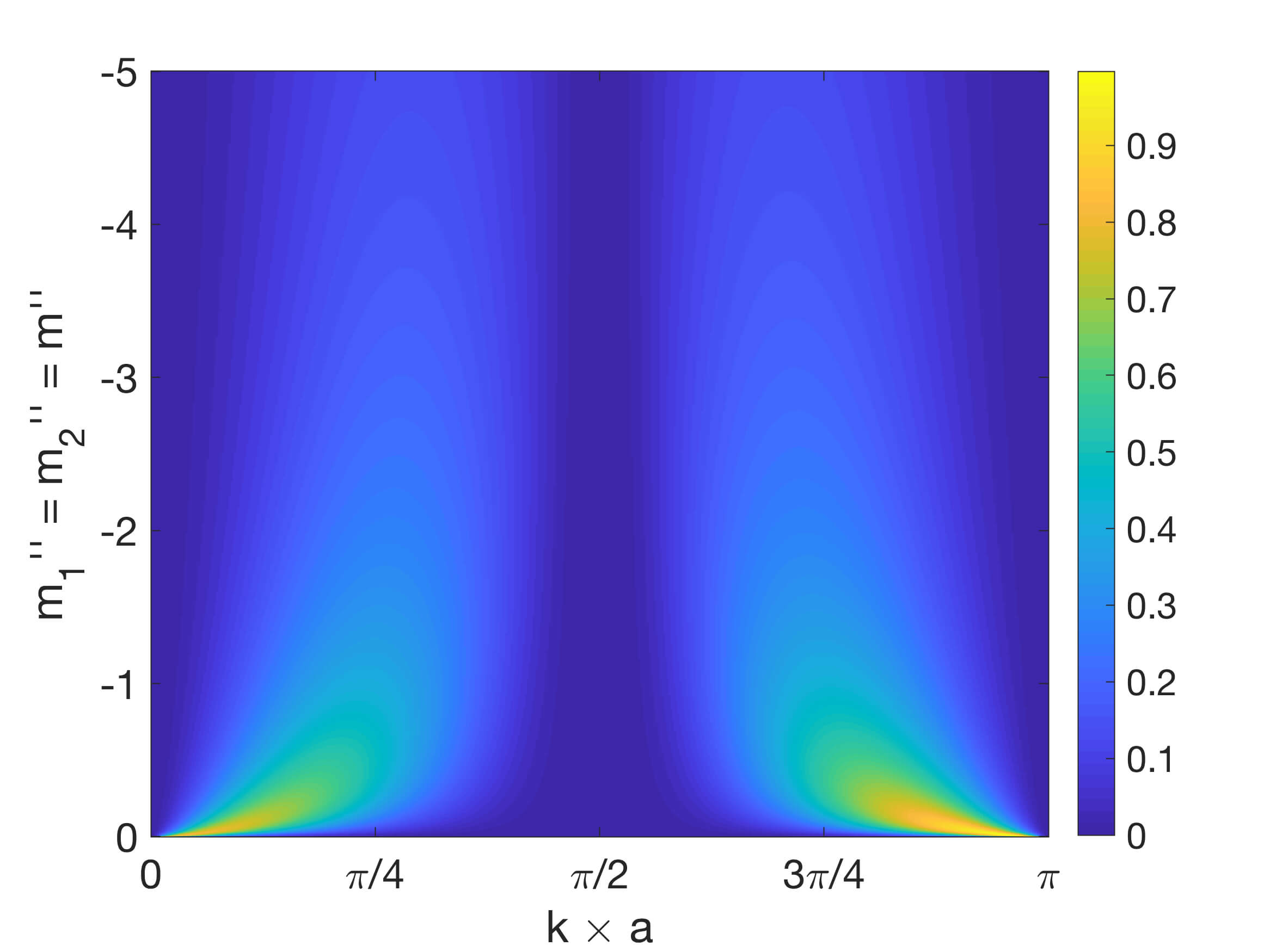
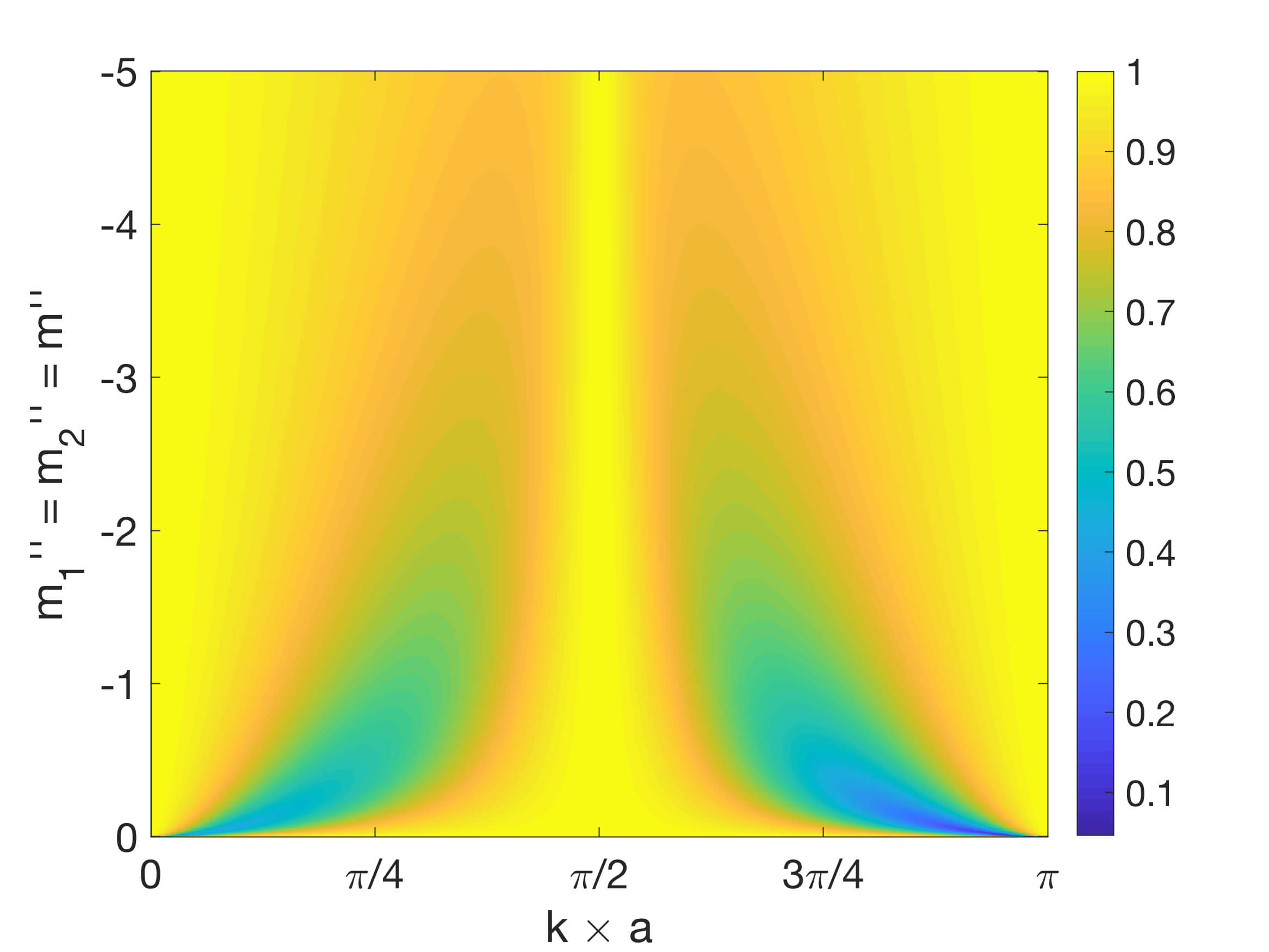
Figure 9: Reflection $|R_{-}|$, (a), and transmission $|T|$, (b), for $m_{1}^{\prime\prime}=m_{2}^{\prime\prime}=m^{\prime\prime}<0$; $|R_{+}|=0$. Note the large reflectivity for small $m^{\prime\prime}$ and for $ka\approx 0,\,\pi$. This phenomenon is examined in Section V.

IV.3.1 Second impedance purely imaginary.

A special case of scatterer configuration can be obtained for $m_{2}^{\prime}=0$. Then, with $m_{1}=m_{1}^{\prime}+\mathrm{i}m^{\prime\prime}$ and $m_{2}=\mathrm{i}m^{\prime\prime}$ we have two scatterers with the same damping properties. Equation (36) reduces to

$$(m_{1}^{\prime})^{2}=-2m^{\prime\prime}K$$ (37)

and uniquely defines the relation between $m^{\prime\prime}$ and $m_{1}^{\prime}$. Equations (35) can be then reduced to

$$m_{1}^{\prime}=K\tan ka,\ \ \ m^{\prime\prime}=-\frac{1}{2}K\tan^{2}ka.$$ (38)

Possible choices of $m_{1}^{\prime}$ as a function of $m^{\prime\prime}$ and $ka$ are shown in figure 10.

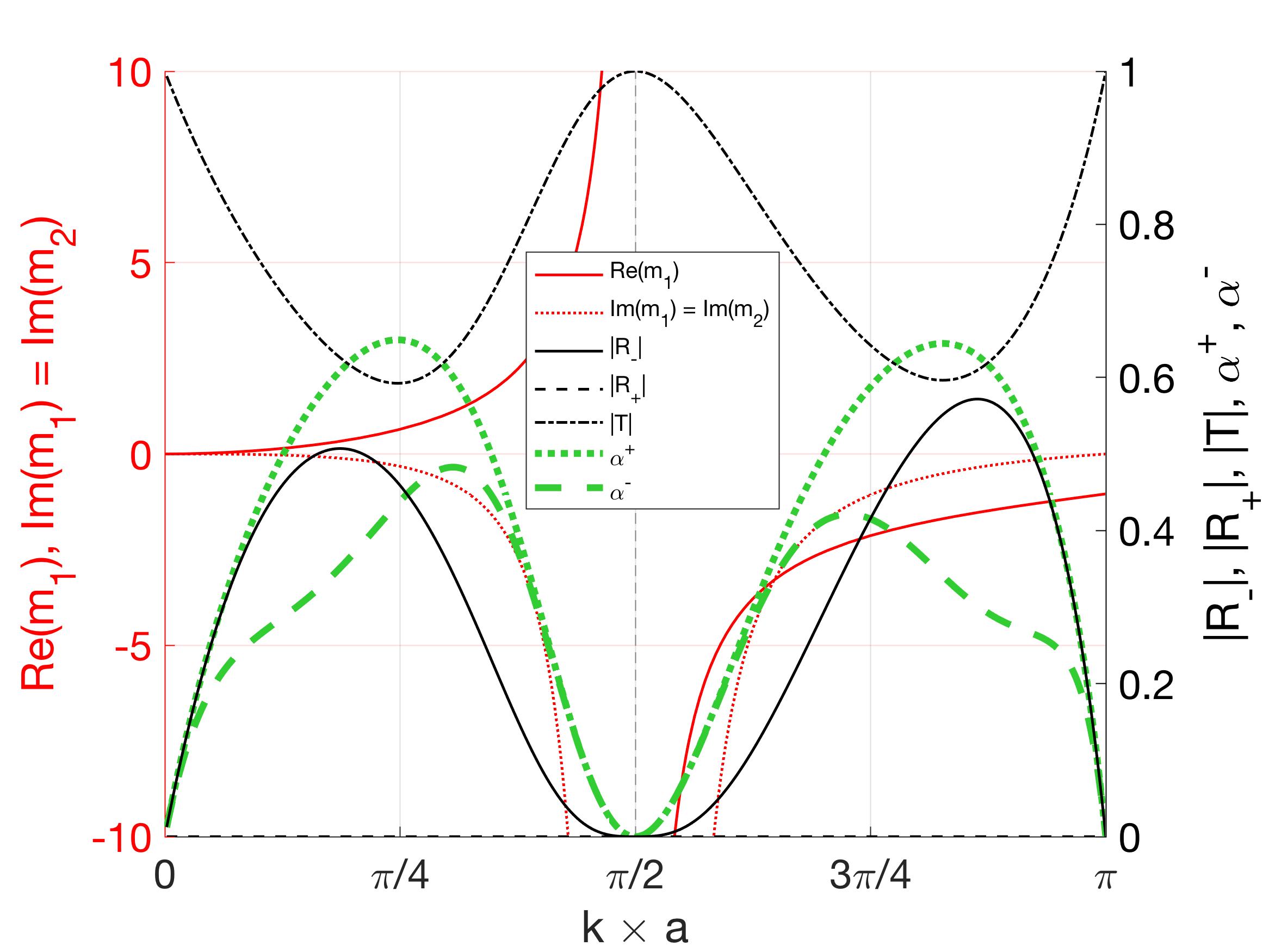
Figure 10: The normalized impedances for zero one-way reflection from equations (38). In this case the two scatterers have the same damping properties, $m_{1}^{\prime\prime}=m_{2}^{\prime\prime}=m^{\prime\prime}$ and $m_{2}^{\prime}=0$.

IV.4 Almost equal impedances.

We now analyze the case where the differences between the real and imaginary parts of the normalized impedances are small. In particular we are interested in the cut of the design space for $m_{-}^{\prime}\approx 0$, as shown by the orange lines in figure 3. We therefore set $m_{-}^{\prime}=\pm\delta$ where $\delta$ is a small number allowing for shifting the cutting plane in the design space; the upper sign is taken for $k\times a\in(0,\pi/2)$ and lower for $k\times a\in(\pi/2,\pi)$, and are required for passive damping, i.e. $m_{+}^{\prime\prime}<0$ where $m_{+}^{\prime\prime}$ follows from (25b). At the same time $m_{-}^{\prime\prime}$ must satisfy $|m_{-}^{\prime\prime}|<-m_{+}^{\prime\prime}$, which is imposed by setting

$$m_{-}^{\prime\prime}=\frac{m_{+}^{\prime\prime}}{c}=\mp\frac{\delta}{c}\tan ka,\ \ \ \ c\in(-\infty,-1)\cup(1,\infty)$$ (39)

with $c\in(-\infty,-1)$ for $m_{-}^{\prime\prime}>0$ and $c\in(1,\infty)$ for $m_{-}^{\prime\prime}<0$, and $m_{+}^{\prime}$ can then be obtained by using (25a). In summary,

$$\begin{aligned} m_{+}&=\big{[}K\mp\delta\big{(}\frac{\tan ka}{c}+\mathrm{i}\big{)}\big{]}\tan ka,\\ m_{-}&=\pm\delta\big{(}1-\mathrm{i}\frac{\tan ka}{c}\big{)},\end{aligned}\ \ \ \text{for }\ \left\{\begin{matrix}k\in(0,\pi/2),\\ k\in(\pi/2,\pi).\end{matrix}\right.$$ (40)

From $m_{-}^{\prime}=\pm\delta$ and (39) it can be seen that for small $\delta$ we have both real and imaginary parts of the normalized impedances nearly the same, regardless of the choice of $c$. Before discussing the case of $k\times a\rightarrow 0$ and $k\times a\rightarrow\pi$ in the next section, we present $m_{1}$ and $m_{2}$ as functions of $k\times a$, required for the zero one-way reflection.

Figure 11 shows the real, $m_{1}^{\prime}$, $m_{2}^{\prime}$, and imaginary, $m_{1}^{\prime\prime}$, $m_{2}^{\prime\prime}$, parts of the normalized complex impedances for two selected combinations of $(\delta,c)$, namely $(1\times 10^{-3},1\times 10^{3})$ (figure 11a) and $(1\times 10^{-3},1)$ (figure 11b), along with reflection and transmission coefficients. For large $c$ (figure 11a) both real and imaginary parts assume nearly the same values over wide $k\times a$ range. For small $c$ (figure 11b), scatterers configurations analogous to those presented in sections IV.1 and IV.2, are obtained with the difference in assumption on the real parts being nonzero and having close values. Note all the configurations presented in figure 11 are passive.

Reflection and transmission coefficients shown in figure 11 display very narrow-band one-way reflection properties. High values of $|R_{-}|$ are observed for $k\times a\rightarrow 0$ and $k\times a\rightarrow\pi$, and are not sensitive to the selection of $c$. Close-up views for $k\times a\rightarrow 0$ and $k\times a\rightarrow\pi$ are shown in figure 12. Note that for $k\times a\rightarrow\pi$ the value of $|R_{-}|$ is close to one, the perfect reflection, while for $k\times a\rightarrow 0$, $|R_{-}|$ converges to a lower value. These surprising results will be analyzed in detail in Section V.

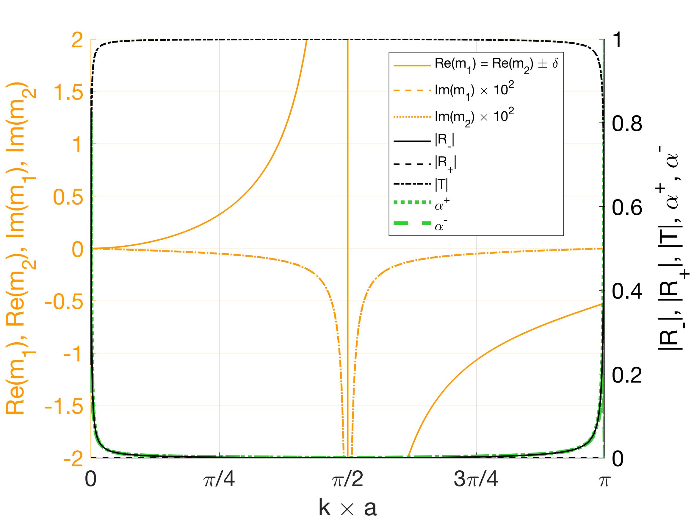
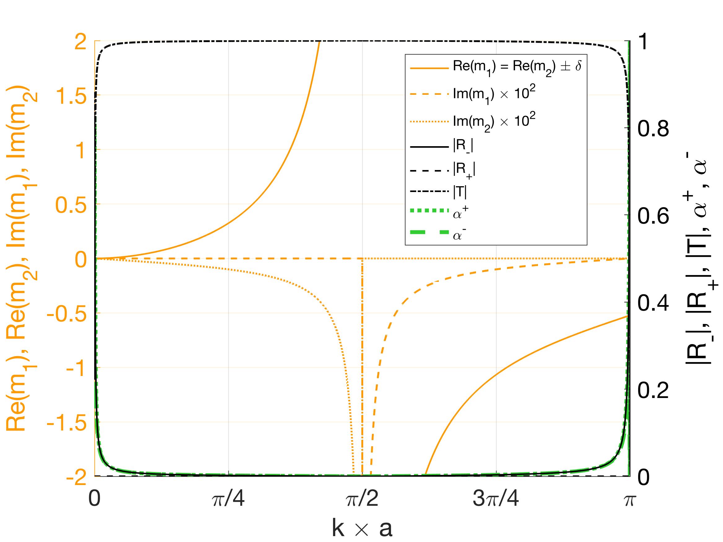
Figure 11: The normalized complex impedances for zero one-way reflection with $\delta=1\times 10^{-3}$ and $c=1000$ (a), and $c=1$ (b). In this case the scatterers share close real and imaginary parts of the complex impedances (a), and close values of the real parts with one of the imaginary parts close to zero (b).

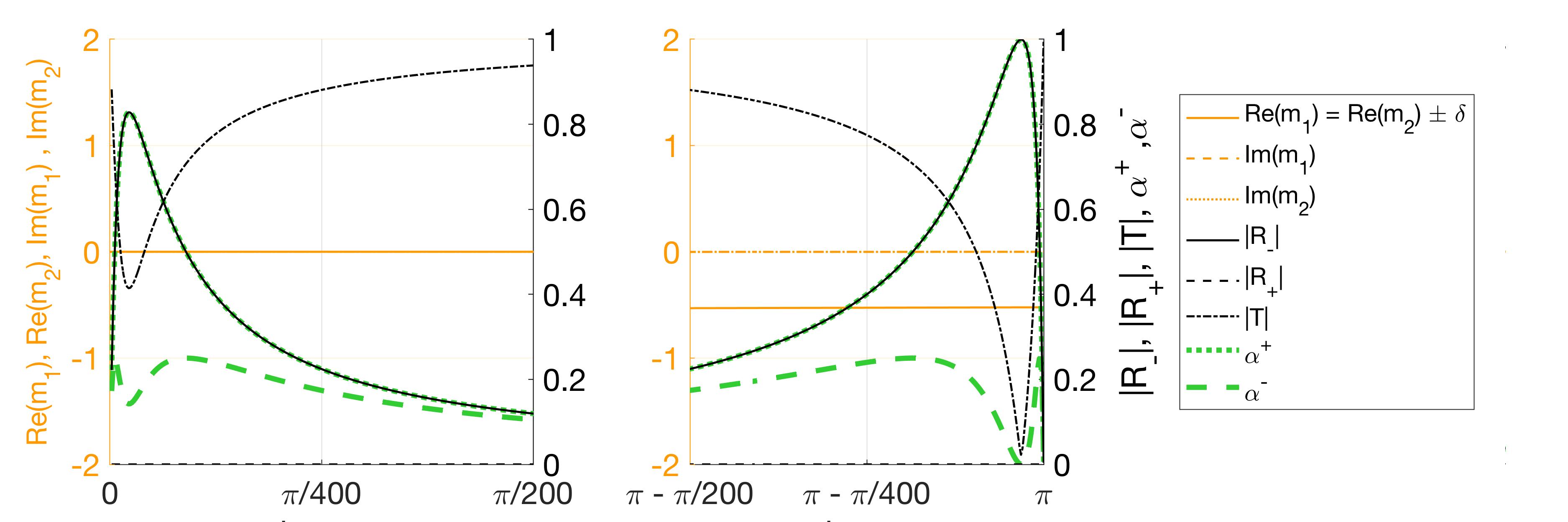
Figure 12: A close-up view of figure 11 (a), ($\delta=1\times 10^{-3}$, $c=1000$), showing the extreme cases of $k\times a\rightarrow 0$ (left) and $k\times a\rightarrow\pi$ (right).

IV.5 Impedances with different passive damping properties.

Selecting an arbitrary, but different from considered so far, configuration of passive damping properties of scatterers we assume - analogously to section IV.4 - that $m_{-}^{\prime\prime}$ and $m_{+}^{\prime\prime}$ are related by $m_{+}^{\prime\prime}=c\ m_{-}^{\prime\prime}$ and $m_{+}^{\prime\prime}<0$. The constant must satisfy $c\in(-\infty,-1)\cup(+1,+\infty)$, where values $c=\{-1;+1\}$ recover results obtained in sections IV.1 and IV.2, and $c=\infty$ is equivalent to result presented in section IV.3. The relation between $m_{+}^{\prime}$ and $m_{-}^{\prime}$ yields

$$\big{(}K-m_{+}^{\prime}\cot ka\big{)}\ c\ \cot ka-m_{-}^{\prime}=0,\ \ \ \ \ m_{+}^{\prime\prime}<0,$$ (41)

Selection of $m_{+}^{\prime\prime}<0$ and $c$ uniquely defines passive damping properties of the two scatterers. Figure 13 presents fragments of the design space for $c<-1$ and $c>1$ for three arbitrarily selected values of $c:|c|=\{\hat{c};10\ \hat{c};100\ \hat{c}\}$, $\hat{c}\geq 1$. It can be seen that for increasingly large values of $|c|$ the shape of the design space converges to that of figure 7, while for small values of $|c|$ to that of figure 3. Specifically, when $|c|$ is large $m_{-}^{\prime\prime}=m_{+}^{\prime\prime}\ /\ |c|\rightarrow 0$, resulting in the same damping properties of the scatterers, and $m_{-}^{\prime}\ /\ |c|\rightarrow 0$ in (41). The latter observations are consistent with results of section IV.3 (see figure 7), and discussion in IV.2.3.

Note that $|m_{-}^{\prime\prime}|<-m_{+}^{\prime\prime}$ with $m_{+}^{\prime\prime}$ and (25b) restrict the selection of $m_{-}^{\prime}>0$ for $k\times a\in(0,\pi/2)$ and $m_{-}^{\prime}<0$ for $k\times a\in(\pi/2,\pi)$. The value of $m_{+}^{\prime}$ is then given by

$$m_{+}^{\prime}=\big{(}K-\frac{m_{-}^{\prime}}{c}\tan ka\big{)}\tan ka.$$ (42)

For negative $|c|$ (figure 13b) $m_{+}^{\prime}$ behaves as $\sim\tan^{2}ka$ for small $|c|$ and as $\sim\tan ka$ for large $|c|$. For small positive $|c|$ (figure 13a) $m_{+}^{\prime}$ takes values $\sim-\tan^{2}ka$ and for large positive $|c|$, $m_{+}\sim\tan ka$. It should be noted that as $m_{+}^{\prime}$ can change its sign, there exists $m_{+}^{\prime}=0$ choice (i.e. equal but opposite real parts of the normalized impedances) and can be achieved by a configuration satisfying

$$m_{-}^{\prime}=cK\cot ka.$$ (43)

It follows from equation (25b) that (43) can be satisfied only by $c>0$ for the system to be passive.

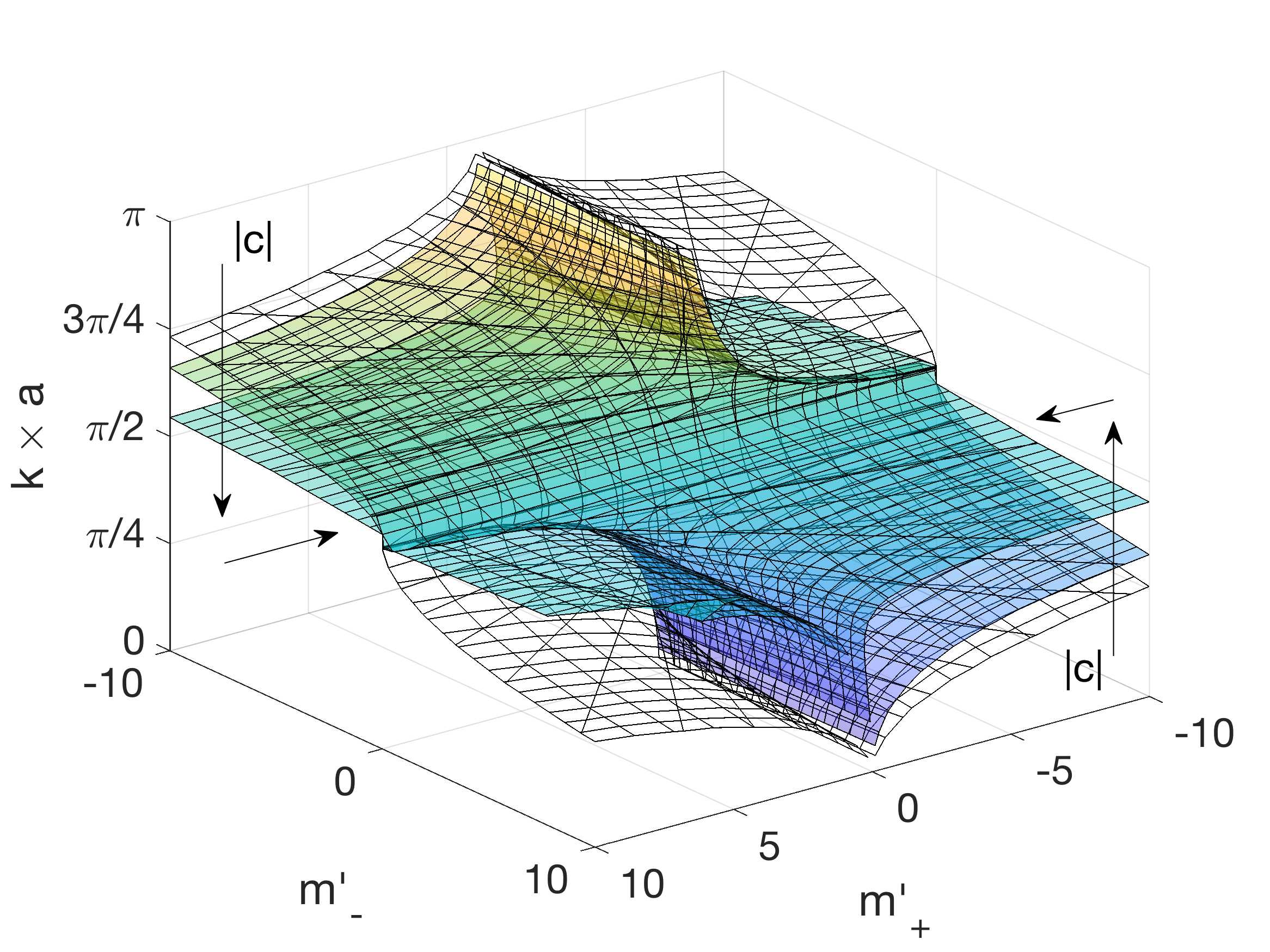
Figure 13: The design space analogous to that from figure 3, defined by equation (41) for $c=\{\hat{c};10\ \hat{c};100\ \hat{c}\}$, (a), and for $c=\{-\hat{c};-10\ \hat{c};-100\ \hat{c}\}$, (b).

V Maximum reflection for $ka\ll 1$ and $ka\approx\pi$

We return to the surprising results indicating that significant one way reflection $(|R_{-}|>0.8)$ is possible for $ka\ll 1$, and that almost unitary one way reflection $(|R_{-}|\approx 1)$ can be achieved for $ka\approx\pi$, as illustrated in figures 9 and 12. Here we derive analytical expressions that help explain the extreme values of $|R_{-}|$. These effects are associated with small imaginary parts for the impedances $-m_{1}^{\prime\prime},-m_{2}^{\prime\prime}\ll 1$; we therefore concentrate on the case considered in Section IV.3 for $m_{1}^{\prime\prime}=m_{2}^{\prime\prime}\equiv m^{\prime\prime}$, corresponding to the impedances defined by Eqs.  (35). The single parameter $m^{\prime\prime}$ yields, from (23c) and (34) a reflection coefficient

$$R_{-}=\frac{2m^{\prime\prime}\cos ka}{\big{(}\frac{m^{\prime\prime}}{\sin ka}+\mathrm{i}g(a)\tan ka\big{)}^{2}}.$$ (44)

Equation (44) may be written as

$$R_{-}=\frac{-\cos ka}{\big{(}\frac{1}{2y}-\frac{\mathrm{i}g(a)y}{\cos ka}\big{)}^{2}}\ \ \text{where }\ y=\frac{\sin ka}{\sqrt{-2m^{\prime\prime}}}.$$ (45)

This form allows us to easily find the asymptotic limits appropriate to the two cases of interest, which are considered next.

V.1 Low frequency maximal absorption

Expanding the expression (45) for $ka\ll 1$, $-m^{\prime\prime}\ll 1$ indicates the preferred scaling $m^{\prime\prime}=$O$(ka)^{2}$. Thus,

$$R_{-}\approx\frac{-4}{\big{(}\frac{1}{\gamma}+(1+\mathrm{i})\gamma\big{)}^{2}}\ \ \text{with}\ \gamma=\frac{ka}{\sqrt{-2m^{\prime\prime}}}.$$ (46)

Hence, $|R_{-}|=4/\big{(}\frac{1}{\gamma^{2}}+2\gamma^{2}+2\big{)}$, implying that the maximum reflection is $R_{-}=2(\sqrt{2}-1)e^{\mathrm{i}3\pi/4}$ at $\gamma=2^{-1/4}$, corresponding to

$$R_{-}=-0.5858+0.5858\,\mathrm{i}=0.8284\,e^{\mathrm{i}3\pi/4}.$$ (47)

In summary, for a given value of $-m^{\prime\prime}\ll 1$ the reflection for small $ka$ is given approximately by (46), with maximum amplitude $|R_{-}|=0.8248$ at $ka=1.1892\sqrt{-m^{\prime\prime}}$. An example is shown in Figure 14.

V.2 Maximal absorption for $ka\approx\pi$

In this case we assume $\pi-ka\ll 1$, $-m^{\prime\prime}\ll 1$. Expanding the expression (45) we find a similar preferred scaling as before, with now $m^{\prime\prime}=$O$\big{(}(\pi-ka)^{2}\big{)}$. Thus,

$$R_{-}\approx\frac{4}{\big{(}\frac{1}{\gamma}+z\gamma\big{)}^{2}}$$ (48)

where

$$\gamma=\frac{\pi-ka}{\sqrt{-2m^{\prime\prime}}},\ \ z=1-\mathrm{i}e^{-\pi}=|z|e^{\mathrm{i}\phi},$$ (49)

i.e.  $|z|=1.0009$, $\phi=-0.0432$. In this case $|R_{-}|=4/\big{(}\frac{1}{\gamma^{2}}+|z|^{2}\gamma^{2}+2\big{)}$, implying that the maximum reflection coefficient is $R_{-}=1/(z\cos^{2}\frac{\phi}{2})$ at $\gamma=|z|^{-1/2}=0.9995$, corresponding to

$$R_{-}=0.9986+0.0432\,\mathrm{i}=0.9995\,e^{-\mathrm{i}\phi}.$$ (50)

The maximum $|R_{-}|$ is very close to, but not equal to unity, as illustrated in the example of Figure 14. In summary, for a given value of $-m^{\prime\prime}\ll 1$ the reflection for $ka\approx\pi$ is given approximately by (48) and (49), with almost unit maximum amplitude at $ka=\pi-1.4136\sqrt{-m^{\prime\prime}}$

Finally, we note from Eqs.  (35) that the impedances for both cases, $ka$ near zero and $\pi$, are

$$m_{1\over 2}\approx\pm\frac{\sqrt{-m^{\prime\prime}/2}}{\gamma}+\mathrm{i}m^{\prime\prime}.$$ (51)

These correspond to lightly damped oscillators, one being an effective mass, the other a stiffness.

Figure 14: Reflection coefficient $|R_{-}|$ near $ka=0$ (left) and $ka=\pi$ (right) for $m_{1}^{\prime\prime}=m_{2}^{\prime\prime}=-0.005$; $|R_{+}|=0$. In both cases the exact coefficient is from (44). The approximation for small $ka$ comes from (46), and for $ka\approx\pi$ from (48). Absorption coefficients $\alpha^{\pm}$ computed for approximate values of $R_{-}$.

VI Maximum reflection for $ka>\pi$

Finally, we consider the unique value of $m_{+}=m_{1}+m_{2}$ for which the transmission is identically zero, $T=0$, in addition to $R_{+}=0$. It follows from eq. (23d) that both $R_{-}$ and $T$ vanish if

$$m_{+}=2g(0)-2g(a)\cos ka-\mathrm{i}2\sin^{2}ka,$$ (52)

implying, using eq. (23), that

$$m_{1} =-\frac{1}{2}+\big{(}\sin ka+\frac{1}{2}e^{-ka}\big{)}e^{-\mathrm{i}ka},$$ (53)

$$m_{2} =-\frac{1}{2}+\frac{1}{2}e^{-ka}e^{\mathrm{i}ka},$$

$$R_{-} =-e^{-\mathrm{i}ka}+\mathrm{i}e^{-ka}.$$

The lowest value of $ka$ for which both impedances are passive $m_{1}^{\prime\prime},m_{2}^{\prime\prime}\leq 0$ is $ka=1.0067\,\pi$, and they remain passive until $ka=2\pi$. Therefore, for almost all of the range $ka=(\pi,2\pi)$ these impedances yield $R_{+}=T=0$ with almost unit amplitude one way reflection $|R_{-}|>0.986$. The damping of attachment 2 is very small, $m_{2}^{\prime\prime}>-0.007$, with almost all the damping in resonator 1.

VII Summary and conclusions

We have presented for the first time a flexural wave analogue of the one-way absorption effect in acoustics. Similar to the acoustic setup, we consider a pair of adjacent lumped elements which breaks the symmetry of the scattering, in this case oscillators attached pointwise on a beam. It is found that at least one of the oscillators must be damped in order to have zero reflection from one direction with significant reflection from the opposite direction. The method of analysis developed in Section II can be easily generalized to handle larger clusters of oscillators; however, we have shown that two are sufficient to achieve one-way absorption.

The starting point for finding possible combinations of oscillator pairs is Eq. (19) which guarantees one reflection coefficient vanishes (in this case $R_{+}=0$). This condition provides a single relation between the normalized impedances $m_{1}=m_{1}^{\prime}+\mathrm{i}m_{1}^{\prime\prime}$ and $m_{2}=m_{2}^{\prime}+\mathrm{i}m_{2}^{\prime\prime}$, which are otherwise unconstrained except that they must correspond to passive oscillators $(m_{1}^{\prime\prime}\leq 0,m_{2}^{\prime\prime}\leq 0)$. This leaves a large set of possible configurations that may be considered. The bulk of the paper, Sections IV and V, is devoted to investigating this large space of design parameters. The numerous examples demonstrate that one way absorption can be realized by various configurations of the scatterers and their mechanical properties, e.g. a combination of a single damper with two mass-spring elements, a damper with a single mass-spring oscillator, a pinned point with a damper or combinations of two dampers with oscillators.

The examples discussed in Section IV and summarized in Table 1 indicate that significant one-way reflection can be obtained for attachments spaced less than $\lambda/2$ apart. For instance, if one of the impedances is real, corresponding to a mass or a stiffness, and the other attachment is a pure damper, then almost unit reflection can be achieved for an approximate spacing of $\lambda/2$ (see Figure 5). Alternatively, if one of the points is pinned and the other attachment is a damped oscillator then relatively broadband and significant one-way reflection is possible, as shown in Figure 6. This finding for flexural waves differs substantially from the acoustic case. Here perfect one-way absorption can be obtained for a combination of a damped oscillator with a pinned point - and is attributed to the partial transfer of elastic waves through the pinned (i.e. $w=0$) point due to rotations of the beam cross sections. We find that virtually perfect one-way absorption is possible with two attachments with the same but small damping, if the spacing between them is slightly less than $\lambda/2$. Such a configuration requires real parts of the scatterers’ impedances of opposite signs (see (51)) and could be achieved by properly selected high values of mass (positive sign) and stiffness (negative sign) parameters for each of them (see (2)). This effect, shown in Figure 14 has also been verified using asymptotics based on the small parameter $m_{1}^{\prime\prime}=m_{2}^{\prime\prime}$. Surprisingly, the same setup of two attachments with equal and small damping yields a reflectivity of magnitude $0.82$ for very small spacing $a\ll\lambda$, also shown in Figure 14. The strictly sub-wavelength nature of this effect means that the pair of damped oscillators may be viewed as a single attachment, i.e.  a flexural wave Willis element Muhlestein2017a .

The results in this paper open up new possibilities in structural wave dynamics. For instance, one could in principle design vibration absorbers that are not only frequency selective, but also depend on where the noise is incident from. In this paper we have shown that a large design space exists; however, there is more work to be done in interpreting this type of phenomenon in terms of realistic adaptive oscillators. This requires mapping the non-dimensional impedances found back to realistic oscillator dynamics, as in the spring-mass-damper models of Eq. (2). The present results use only translational impedances (point forces) in the context of the classical beam theory, but could be extended to include concentrated moments and more refined engineering theories. For instance, further analysis of the results in Section V.1 in which the point attachments are very close together would benefit from a more precise theory, such as Timoshenko’s, that better models the near-field of concentrated forces.

References

- (1) Michael B. Muhlestein, Caleb F. Sieck, Preston S. Wilson, and Michael R. Haberman. Experimental evidence of Willis coupling in a one-dimensional effective material element. Nature Comm., 8:15625, Jun 2017.
- (2) Xiaoshi Su and Andrew N. Norris. Retrieval method for the bianisotropic polarizability tensor of Willis acoustic scatterers. Physical Review B, 98(17), Nov 2018.
- (3) Aurélien Merkel, Vicent Romero-Garciá, Jean-Philippe Groby, Jensen Li, and Johan Christensen. Unidirectional zero sonic reflection in passive PT -symmetric Willis media. Physical Review B, 98(20), nov 2018.
- (4) D. J. Mead. Structural wave motion, chapter 9 in Noise and Vibration, R. G. White and J. G. Walker (editors), pages 207–226. Ellis Horwood Publishers, Chichester, 1982.
- (5) M J Brennan. Vibration control using a tunable vibration neutralizer. Proceedings of the Institution of Mechanical Engineers, Part C: Journal of Mechanical Engineering Science, 211(2):91–108, feb 1997.
- (6) M.J. Brennan. Control of flexural waves on a beam using a tunable vibration neutraliser. Journal of Sound and Vibration, 222(3):389–407, may 1999.
- (7) H.M. El-Khatib, B.R. Mace, and M.J. Brennan. Suppression of bending waves in a beam using a tuned vibration absorber. Journal of Sound and Vibration, 288(4-5):1157–1175, dec 2005.
- (8) Cheng Yang and Li Cheng. Suppression of bending waves in a beam using resonators with different separation lengths. Journal of the Acoustical Society of America, 139(5):2361–2371, may 2016.
- (9) Daniel Torrent, Didier Mayou, and José Sánchez-Dehesa. Elastic analog of graphene: Dirac cones and edge states for flexural waves in thin plates. Physical Review B, 87(11), mar 2013.
- (10) D. V. Evans and R. Porter. Penetration of flexural waves through a periodically constrained thin elastic plate in vacuo and floating on water. Journal of Engineering Mathematics, 58(1):317–337, Aug 2007.