Deep learning for presumed probability density function models

Abstract

In this work, we use machine learning (ML) techniques to develop presumed probability density function (PDF) models for large eddy simulations of reacting flows. The joint sub-filter PDF of mixture fraction and progress variable is modeled using various ML algorithms and commonly used analytical models. The ML algorithms evaluated in the work are representative of three major classes of ML techniques: traditional ensemble methods (random forests), deep learning (deep neural network s), and generative learning (conditional variational autoencoder (CVAE)). The first two algorithms are supervised learning algorithms, and the third is an unsupervised learning algorithm. Data from direct numerical simulation of the low-swirl burner [1] are used to develop training data for sub-filter PDF models. Models are evaluated on predictions of the sub-filter PDFs as well as predictions of the filtered reaction rate of the progress variable, computed through an integral of the product of the sub-filter PDF and the conditional means of the reaction rate. This a-priori modeling study demonstrates that deep learning models for presumed PDF modeling are three times more accurate than analytical $\beta$-$\beta$ PDF models and linear regression models. These models are as accurate as random forest models while using five times fewer trainable parameters and being 25 times faster for inference. In this work, conditional unsupervised learning did not present additional advantages beyond supervised learning with a feed-forward neural network. We illustrate how models generalize to other regions of the flow and develop criteria based on the Jensen-Shannon divergence to quantify the performance of a model on new data.

1 Introduction

Simulation has the potential to accelerate the development of cost-effective combustion technologies. Even with modern high-performance computing hardware however, the computational cost of fully resolving the reacting flows in these devices can be prohibitive. Large eddy simulations (LES) reduce the computational burden of simulating turbulent reacting flows. LES work with spatially filtered state variables, which exhibit considerably less temporal and spatial structure and thus require much less numerical resolution. However, physical processes occurring at scales smaller than the filter width must then be approximated with “closure models,” which of course then determine the accuracy of the approach. LES closure models for nonreacting flows have received a great deal of recent attention, and they are now in standard use for a wide range of engineering applications. For reacting flows, considerable complexity arises from the necessity to incorporate additional fine scales because of chemical processes and chemistry-turbulence interactions. One approach to constructing sub-filter LES models for reacting flows is to express modeled quantities as weighted integrals between the physical state and a probability density function (PDF). A presumed PDF approach posits a class of parameterized functional shapes for such PDFs, and thus it defines a parameterized model based on the resulting weighted integrals. In some of the earliest work in this area, Cook and Riley [2] proposed the use of $\beta$ functions for the PDF shape for a conserved scalar such as mixture fraction; much of the work in the field since then has followed this basic strategy. Jiménez et al. [3] provided further analysis to justify the appropriateness of the $\beta$ PDF for passive scalar mixing. Bradley et al. [4, 5] investigated a mixedness-reactedness formalism to increase model fidelity. Ihme and Pitsch [6, 7] determined that the “statistically most likely distribution” was most appropriate for a reacting scalar case.

The objective of the work presented here is to expand on the presumed $\beta$ approach, with specific focus on the case of reacting scalars. We incorporate a variety of machine learning (ML) algorithms to explore the accuracy of a number of PDF shape functionals for their use with an LES model, and we judge them by their ability to reproduce a large-scale, direct numerical simulation (DNS) data set for a specific reacting flow configuration. We explore three major classes of ML algorithms for use in this context: traditional ensemble methods (random forests); deep learning (deep neural network); and deep, generative, unsupervised learning (conditional variable autoencoder). More broadly, traditional ML methods include techniques such as linear and polynomial regression, k-nearest neighbors, support vector machines, Gaussian processes, and random forests. Of these, we focus only on the latter because they have demonstrated widespread success for complex modeling applications [8, 9]. Random forests are based on an ensemble of decision trees, where decisions are based on the model parameters to provide estimates of the target. Deep neural networks (DNNs) are universal function approximators [10, 11] based on a sequence of learnable linear operators and activation functions that are tuned using a gradient-descent optimizer. DNNs have received much attention in recent years, in large part because of the availability of large public training data sets and powerful computing platforms such as graphics processing units (GPUs) [12]. Additional advances in deep learning, particularly in the types of neural network architectures, have led to breakthroughs in generative and unsupervised learning, where new data are generated using the models with unlabeled data and then by identifying trends and commonalities in the generated data. Variational auto-encoders (VAEs) leverage neural networks to encode information from input data into a latent space, which can then be sampled through a decoder to generate new distributions that are similar to the original data set.

In this work, we use the three ML approaches discussed here to construct presumed PDF models for a DNS data set that is a snapshot of a quasi-stationary simulation of a low-swirl, premixed methane-air burner [1]. We then evaluate the suitability of the different classes of ML algorithms, and of the presumed PDF model itself, both for data from a subregion of the DNS and for the entire simulation domain. In Section 2, we formulate the target problem and methods, including the details of the presumed PDF approach, the DNS target data, and the ML algorithms and network architectures explored. In Section 3, we compare the ML-based constructions to simple analytic models.

2 Formulation

2.1 Presumed probability density function modeling for combustion

In LES of reacting flows using presumed forms of PDFs, an important unclosed term in the equations is the filtered reaction rates, appearing as a source term in the transport equation for species mass fractions or progress variables [13, 14]. A common approach to modeling the filtered reaction rates is to express it as an integral of the product of a reaction rate derived from a physical model and a PDF. The conditioning variables are typically chosen to correlate strongly with mixing (mixture fraction) and flame propagation (progress variable) space [4, 5], accounting for much of the subgrid variation about the mean. The conditional rate can then be modeled through a variety of approaches to identify the manifold, such as canonical calculations and tabulation (e.g., flamelet-generated manifolds [15], flame prolongation of intrinsic low dimensional manifold [16]), solving conditional transport equations (e.g., conditional moment closure [17]), or estimated on the fly using conditional source term estimation [18]. Once the conditional rate is obtained, through whatever means, the unconditional mean that appears in the source term for the transport equations can be recovered by weighting with the distribution and integrating over the conditioning space:

$$\widetilde{\dot{\omega}}=\int\langle\dot{\omega}|Z,c\rangle P(Z,c|\widetilde{Z},\widetilde{Z^{\prime\prime}},\widetilde{c},\widetilde{c^{\prime\prime}})\,\mathrm{d}Z\,\mathrm{d}c.$$ (1)

Here, $\langle\cdot\rangle$ denotes the volumetric mean of a quantity; $\widetilde{\cdot}=\nicefrac{{\overline{\rho~{}\cdot}}}{{\overline{\rho}}}$ denotes the Favre filter; $\overline{\cdot}$ denotes the LES filter; $Z$ is the mixture fraction, capturing the mixing of fuel and oxidizer; $c$ is the progress variable, capturing the overall reaction progress; $\dot{\omega}$ is the reaction rate of the progress variable (units of $\nicefrac{\mathrm{1}}{\mathrm{s}}$, omitted for brevity); $Z^{\prime\prime}=(Z-\widetilde{Z})^{2}$ is the square of the mixture fraction subgrid scale fluctuation; $c^{\prime\prime}=(c-\widetilde{c})^{2}$ is the square of the progress variable subgrid scale fluctuation; and $P(Z,c|\widetilde{Z},\widetilde{Z^{\prime\prime}},\widetilde{c},\widetilde{c^{\prime\prime}})$ is the density-weighted PDF of $Z$ and $c$, conditioned on $\widetilde{Z}$, $\widetilde{Z^{\prime\prime}}$, $\widetilde{c}$, and $\widetilde{c^{\prime\prime}}$. It should be noted that the ML models presented in this study are being trained using realizations of the filtered probability density function (FPDF), referred to as filtered density functions (FDFs), computed from the DNS data and which are characterized by the subgrid means and variances. This distinction between FPDFs and FDFs will be adhered to throughout this work and follows the convention presented by Fox [19], Pitsch [14]. The objective of this work is to develop accurate models to generate FPDFs for LES using ML techniques trained on FDFs from the DNS data set. Current analytical models often rely on using a $\beta$ PDF [2]. Though $\beta$-$\beta$ model is based on a physically satisfying limiting behavior and is an established presumed PDF model, the model is not universal and there is ongoing research to improve the presumed PDF modeling approach [20, 21, 22]. The $\beta$ PDF is defined as:

$$\beta(x;a,b)=\frac{\Gamma(a+b)}{\Gamma(a)\Gamma(b)}x^{a-1}(1-x)^{b-1},$$ (2)

where $\Gamma(\cdot)$ is the gamma function; $a$ and $b$ are the $\beta$ PDF parameters, which can be related to the mean, $\mu$, and variance, $\sigma^{2}$, as $a=\mu\left(\frac{\mu(1-\mu)}{\sigma^{2}}-1\right)$, and $b=(1-\mu)\left(\frac{\mu(1-\mu)}{\sigma^{2}}-1\right)$. In this work, $\widetilde{Z}$ and $\widetilde{Z^{\prime\prime}}$ are used as the mean and variance for a $\beta$ PDF in the mixture fraction space, and $\widetilde{c}$ and $\widetilde{c^{\prime\prime}}$ form the $\beta$ PDF in the progress variable space, such that $P(Z,c)=\beta(Z;a_{\widetilde{Z}},b_{\widetilde{Z}})\beta(c;a_{\widetilde{c}},b_{\widetilde{c}})$. The form of this expression for the $\beta$-$\beta$ model was chosen to be the product of two marginal $\beta$ PDFs because it is the simplest closed-form analytical expression resulting from using the first and second moments of the input variables. Other expressions, such as the “statistically most likely distribution” [6] or the generalized Dirichlet distribution approach, could have been chosen though these result in unclosed analytical forms requiring the solution of non-linear equations at each grid point. Furthermore, following the Connor-Mosimann approach and assuming unit-square support for the two input variables results in the same product of two marginal $\beta$ PDFs chosen for this work [23]. Therefore, this model will be used for comparisons with data-driven models using different ML techniques.

2.2 Description of the direct numerical simulation of the low-swirl burner

The DNS of an experimental lean premixed turbulent low-swirl methane flame provide the data for model development [1, 24]. In this configuration, a nozzle imposes a low swirl (geometric swirl number of 0.55) to a CH₄ and air mixture with a fuel-air equivalence ratio of 0.7 at the inflow, Figure 1. A co-flow of cold air surrounds the nozzle region with an upward velocity of $0.25\,\nicefrac{\mathrm{m}}{\mathrm{s}}$. The inflow velocity of the fuel-air mixture at the nozzle is $15\,\nicefrac{\mathrm{m}}{\mathrm{s}}$. The laminar flame thickness is $600\,\mathrm{\mu m}$. The simulation was performed using LMC, a low Mach number Navier-Stokes solver for turbulent reacting flows that leverages adaptive mesh refinement to resolve finer scales [25]. Three levels of refinement were used, leading to effective resolution of $100\,\mathrm{\mu m}$ in the flame region. The computational domain was $0.25\,\mathrm{m}$ in each dimension. The DRM 19 chemical mechanism was used to model the finite rate kinetics [26]. The domain pressure is $1\,\mathrm{atm}$. The physical characteristics and the mechanisms behind the flame are discussed in detail by Day et al. [1] and will not be described here for brevity.

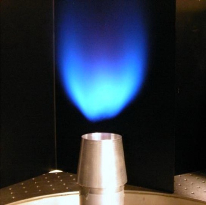
Figure 1: Lifted flame of the low-swirl burner from the experimental configuration. From Day et al. [1]. © Elsevier. Reproduced with permission.

In the current analysis, the mixture fraction, $Z$, is computed through a linear combination of the nitrogen mass fraction in the burner exit stream and the co-flow and it is normalized such that it varies between 0 in the co-flow stream and 1 in the burner exit stream. The mixture fraction variable is used to quantify the mixing between the stream from the fuel nozzle and the co-flow. When defined this way, the mixture fraction variable has no relation to the local fuel mass fraction and is a passive scalar with a transport equation comprising only of temporal, advection, diffusion, and sub-grid turbulent mixing terms. The progress variable is defined in this work as $c=Y_{CO_{2}}+Y_{CO}+Y_{H_{2}}+Y_{H_{2}O}$ and varies between 0 and 0.21, where $Y_{i}$ is the mass fraction of species $i$, $\sum^{N_{s}}_{i=1}Y_{i}=1$, and $N_{s}$ is the number of species. This definition of progress variable leads to a simpler transport equation for the progress variable than a temperature based progress variable or any other species mass fractions based progress variable. This work is focused on determining models for the joint FDF and, thus, does not require the independence of the mixture fraction and the progress variable.

The primary motivation behind choosing this test case to demonstrate the capabilities of ML for joint FDF models is the presence of multiple burning regimes. As seen in Figure 2, a premixed flame lifted from the fuel nozzle is clearly observed. The products from this premixed flame mix downstream with the air from the co-flow, which sets up a secondary reacting zone. A number of modeling challenges are introduced because of the presence of these multiple regimes. One of these modeling challenges is to capture the joint FDF describing the mixing of the mixture fraction, a passive scalar, with the progress variable, an active scalar. Analytical models for joint FDFs have found to be lacking accuracy for such complex configurations [6], and, this motivates the exploration of ML techniques for constructing models for challenging turbulent combustion problems, such as the configuration considered in this study. Additional advantages of using data from multiple burning regimes for training ML models include using of more diverse training data, avoiding overfitting, and increasing the opportunities for model generalization.

(a) $x=0\,\mathrm{m}$.

(b) $z=0.0525\,\mathrm{m}$ (center height of $\mathcal{V}_{1}$).

(c) $z=0.0775\,\mathrm{m}$ (center height of $\mathcal{V}_{3}$).

(d) $z=0.1025\,\mathrm{m}$ (center height of $\mathcal{V}_{5}$).

(e) $z=0.1275\,\mathrm{m}$ (center height of $\mathcal{V}_{7}$).

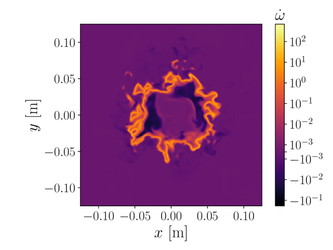
(f) $z=0.14\,\mathrm{m}$ (center height of $\mathcal{V}_{9}$).

Figure 2: Slices of $\dot{\omega}$ in DNS. White dashed lines: $z$ locations of slices shown in (b)–(f).

(a) $\widetilde{Z}$.

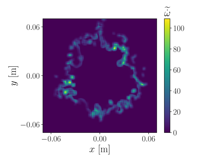
(b) $\widetilde{Z^{\prime\prime}}$.

(c) $\widetilde{c}$.

(d) $\widetilde{c^{\prime\prime}}$.

Figure 3: Slices of filtered DNS data at $z=0.0775\,\mathrm{m}$ (center height of $\mathcal{V}_{3}$).

2.3 Generation of the modeling data

A data set of sample moments and associated FDFs was generated from a statistically stationary single time snapshot at $t=0.0626\,\mathrm{s}$ from this DNS by considering different sub-volumes of the domain that span the flame, from the region of premixed burning of the fuel-air mixture from the nozzle to the mixing zone between the products from the primary premixed flame and the air from the co-flow. These volumes — denoted by $\mathcal{V}_{i}$, where $i=1,\dots,n_{v}$ and $n_{v}=9$ is the number of sub-volumes — are centered at $z_{i}=0.0525\,\mathrm{m}+(i-1)0.0125\,\mathrm{m}$, with height $0.00625\,\mathrm{m}$ and width $0.14\,\mathrm{m}$, composed of $1146\times 1146\times 51$ cells. The locations of several of these subregions and planar slices of $\dot{\omega}$ are presented in Figure 2. The premixed lifted flame, with high values of $\dot{\omega}$ and steep gradients corresponding to a thin flame, can be observed around $z=0.05\,\mathrm{m}$. Farther downstream of the nozzle, the premixed flame products mix with the air coming from the co-flow and react to produce lower values of $\dot{\omega}$. Representative slices of the filtered DNS data in $\mathcal{V}_{3}$ are presented in Figure 3. The core of the flame is fully burned as seen by high values of $\widetilde{c}$, and the reactions take place in a thin region at the interface of the fuel-air mixture from the nozzle and co-flow air.

Throughout this work, samples refer to a pointwise sampling of the filtered fields, each with an associated collection of moments and an FDF; volumes refer to a subset of the samples divided according to regions of the domain; and the FDF for each sample is described by the four sample moments, $\left[\widetilde{Z},\widetilde{Z^{\prime\prime}},\widetilde{c},\widetilde{c^{\prime\prime}}\right]$. In each volume, sample moments and associated FDFs were generated by using a discrete box filter:

$$\overline{\phi}(x,y,z)=\frac{1}{n_{f}^{3}}\sum_{i=-\nicefrac{{n_{f}}}{{2}}}^{\nicefrac{{n_{f}}}{{2}}}\sum_{~{}j=-\nicefrac{{n_{f}}}{{2}}}^{\nicefrac{{n_{f}}}{{2}}}\sum_{~{}k=-\nicefrac{{n_{f}}}{{2}}}^{\nicefrac{{n_{f}}}{{2}}}\phi(x+i\Delta x,y+j\Delta x,z+k\Delta x)$$ (3)

where $\phi$ is the variable to be filtered, $n_{f}=\nicefrac{{\overline{\Delta}}}{{\Delta}}$ is the number of points in the discrete box filter, $\overline{\Delta}=32\Delta x$ is the filter length scale, and $\Delta x=100\,\mathrm{\mu m}$ is the smallest spatial discretization in the DNS (six times smaller than the laminar flame thickness). The filter length scale was chosen to be representative of typical LES filter scales [14] and to ensure an adequate sampling of the FDF at the filter scale. These filters were equidistantly spaced at $8\Delta x$, leading to 58800 FDFs for each volume. The computed conditional FDFs are the density-weighted FDFs of $Z$ and $c$, discretized with 64 bins in $Z$ and 32 bins in $c$. For notational convenience, $P(Z,c)=P(Z=Z^{*},c=c^{*})$ will be used in this work, and the discrete density functions will be referred to as density functions instead of mass functions. The conditional means of the reaction rate, $\langle\dot{\omega}|Z,c\rangle$, are also computed for each sample with an identical discretization.

Examples of $P(Z,c)$ and $\langle\dot{\omega}|Z,c\rangle$ in $\mathcal{V}_{3}$ for increasing $\widetilde{\dot{\omega}}$ illustrate the wide range of observed shapes, Figure 4. For high $\widetilde{\dot{\omega}}$, the conditional means of $\dot{\omega}$ peak at $c=0.16$ and exhibit a bimodal distribution at high $Z$ because of the burning of the fuel stream from the nozzle ($Z=1$) and the burning of the products mixing with the co-flow. For intermediate $\widetilde{\dot{\omega}}$, the conditional means of $\dot{\omega}$ are largest at $Z=0.7$ and $c=0.14$, which is also attributed to the burning of the mixed products. As $\widetilde{\dot{\omega}}$ increases, the location of the peak of $P(Z,c)$ increases in the $Z$ and $c$ space because reactions happen at higher $Z$ and $c$.

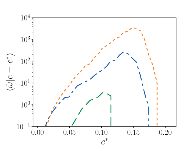
(a) Marginal $P(Z,c)$ as a function of $Z$.

(b) Marginal $P(Z,c)$ as a function of $c$.

(c) Marginal conditional means of $\dot{\omega}$ as a function of $Z$.

(d) Marginal conditional means of $\dot{\omega}$ as a function of $c$.

Figure 4: Examples of $P(Z,c)$ and $\langle\dot{\omega}|Z,c\rangle$ for increasing $\widetilde{\dot{\omega}}$. Red solid: $\widetilde{\dot{\omega}}=0$ ($\widetilde{Z}=0$, $\widetilde{Z^{\prime\prime}}=0$, $\widetilde{c}=0$, $\widetilde{c^{\prime\prime}}=0$); green dashed: $\widetilde{\dot{\omega}}=0.03$ ($\widetilde{Z}=0.4$, $\widetilde{Z^{\prime\prime}}=0.006$, $\widetilde{c}=0.03$, $\widetilde{c^{\prime\prime}}=0.0006$); blue dash-dotted: $\widetilde{\dot{\omega}}=7.4$ ($\widetilde{Z}=0.7$, $\widetilde{Z^{\prime\prime}}=0.01$, $\widetilde{c}=0.08$, $\widetilde{c^{\prime\prime}}=0.003$); orange short dashed: $\widetilde{\dot{\omega}}=42.2$ ($\widetilde{Z}=0.9$, $\widetilde{Z^{\prime\prime}}=0.003$, $\widetilde{c}=0.12$, $\widetilde{c^{\prime\prime}}=0.005$).

Figure 5 illustrates the distribution of moments, $\left[\widetilde{Z},\widetilde{Z^{\prime\prime}},\widetilde{c},\widetilde{c^{\prime\prime}}\right]$, across the samples in $\mathcal{V}_{3}$. Most FDFs are associated with fully burned states originating from the premixed burning of the fuel-air mixture from the nozzle ($\delta$ PDFs centered at $\left(\widetilde{Z},\widetilde{c}\right)=(1,0.2)$) or the nonreacting unburned states ( $\delta$ PDFs centered at and $(0,0)$). A significant number of the FDFs, however, are associated with intermediate states spanning the full range of $\widetilde{Z}$ and $\widetilde{c}$ with larger $\widetilde{Z^{\prime\prime}}$ and $\widetilde{c^{\prime\prime}}$ because of the burning of the products from the primary premixed flame zone mixed with the air from the co-flow.

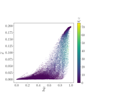
Figure 5: Scatter plots of moments $\widetilde{Z}$ and $\widetilde{c}$ for samples in $\mathcal{V}_{3}$ (centered at $z=0.0775\,\mathrm{m}$) colored by $\widetilde{Z^{\prime\prime}}$ (left) and $\widetilde{c^{\prime\prime}}$ (right) with associated marginal distributions.

2.4 Machine learning algorithms

In this work, we evaluate the performance and suitability of three different types of ML algorithms, each representative of a prevalent class in ML: (i) random forest for traditional ML, (ii) feed-forward DNN for deep learning, and (iii) conditional variational autoencoder (CVAE) for generative and unsupervised learning. The model hyperparameters are summarized in A.

The model inputs are the four sample moments, $\left[\widetilde{Z},\widetilde{Z^{\prime\prime}},\widetilde{c},\widetilde{c^{\prime\prime}}\right]$, and the outputs are the 2048 discrete points representing the joint FDF ($64$ in $Z$, $32$ in $c$). The samples from a volume, $\mathcal{V}_{i}~{}(i=1,\dots,n_{v})$, are randomly distributed among two distinct data sets: a training data set, $\mathcal{D}_{i}^{t}$, used to train the algorithms; and a validation data set, $\mathcal{D}_{i}^{v}$, used to validate the algorithms and comprising $5\%$ of the samples, i.e., $|\mathcal{D}_{i}^{v}|=2940$, where $|\cdot|$ denotes the cardinality of the data set. Figure 6 illustrates this process for $\mathcal{V}_{5}$. In this work, we evaluate different models using different training strategies:

1. Models trained using $\mathcal{D}_{3}^{t}$ and evaluated on $\mathcal{D}_{i}^{v}$ ($i=1,\dots,n_{v}$);

2. Models trained using $\mathcal{D}_{5}^{t}$ and evaluated on $\mathcal{D}_{i}^{v}$ ($i=1,\dots,n_{v}$);

3. Models trained using $\mathcal{D}^{t}=\bigcup\limits_{i=1,3,5,7,9}\mathcal{D}_{i}^{t}$ and evaluated on $\mathcal{D}_{i}^{v}$ ($i=1,\dots,n_{v}$).

The first two strategies involve training and validating on different physical regions of the flame. The third strategy uses training data from the entire flame and the validation data from the training regions and intermediate regions. Prior to training, the sample moments were independently scaled by subtracting the median and dividing the data by the range between the $25^{\text{th}}$ and $75^{\text{th}}$ quantiles. This scaling is robust to outliers [27]. A separate scaling was computed for each training data set and applied to the associated validation data set. The evaluation of a model $m$ on a data set $\mathcal{D}$ is denoted $m(\mathcal{D})$.

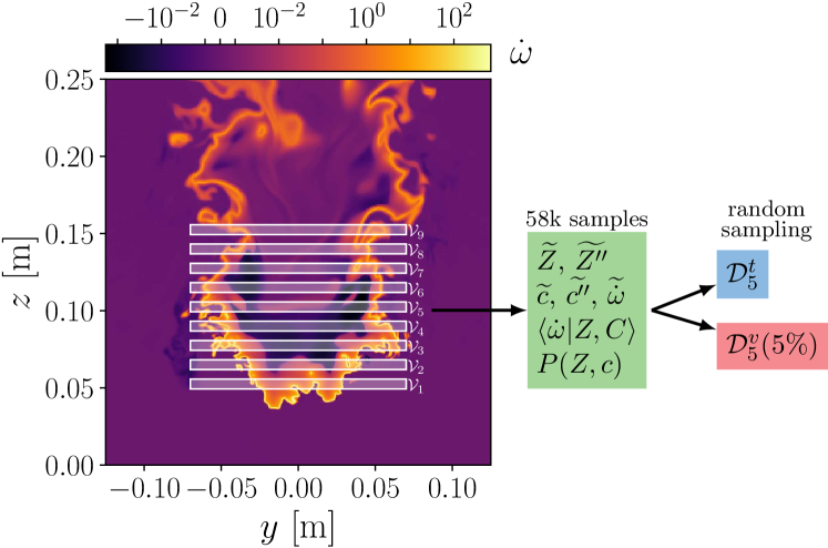
Figure 6: Illustration of data generation procedure for $\mathcal{V}_{5}$.

The first of the investigated models, random forests (RF), is an ensemble model that creates ensembles of low-bias/high-variance individual decision trees and uses the average of the individual model predictions to provide the prediction for the overall forest [28]. A decision tree is a model that uses a treelike structure to represent nodes that encode conditions based on the input variables, branches that split from each node, and termination points, i.e., leaves, which provide the target value predictions, Figure 7(a). The main parameter for a decision tree model is the maximum tree depth, which is the length of the longest path from the root of the tree to a leaf.

Two key insights have driven the effectiveness of random forests models for complex tasks while avoiding overfitting [8, 9], a problem arising when a model is overly accurate on the training data while failing to predict non-training data. The first is that it leverages bootstrap aggregating or bagging, a method that improves model stability, accuracy, and overfitting problems by dividing the training set into several smaller training sets, called bootstraps, populated through random uniform sampling with replacement. In random forests, each decision tree is built using a different bootstrap of the training data. The second is that, instead of splitting each node in the tree according to the best split of all the variables, the split is done using the best split among a random subset of the variables. The two key parameters of the random forests algorithm are the number of decision trees and the depth of the decision trees. For this work, the random forests model contains 100 decision trees and a maximum tree depth of 30 nodes, beyond which results were insensitive to the model size, and the model size grew larger than can be effectively trained on what we consider a typical analysis workstation with 256 GB of memory. The total model degrees of freedom (DoFs), measured as the sum of nodes in each tree, is 5.2 million. Though no constraints were explicitly imposed on the outputs of the random forest model, the model predictions exhibited properties of PDFs (integration to unity and bounded between zero and one).

The field of deep learning has exhibited success in developing models for tasks ranging from image processing [29, 30, 31, 32, 33, 34, 35] to text generation [36, 37, 38] and games [39]. Several reviews of the field give a summary of recent breakthroughs and developments [40, 41, 42, 12, 43]. As a first example of deep learning, we develop a feed-forward, fully connected DNN for presumed PDF modeling. Similar to the decoder network presented below, this network consists of two hidden layers and an output layer. The hidden layers comprise, respectively, 256, and 512 fully connected nodes, a leaky rectified linear unit activation function:

$$y=R(x)=\begin{cases}x,&\text{ if }x\geq 0,\\ \alpha x,&\text{ otherwise, }\end{cases}$$ (4)

where $x$ is the layer input vector, $y$ is the layer output vector, and $\alpha=10^{-2}$ is a small slope; and a batch normalization layer [44]:

$$y=B(x)=\gamma\frac{x-\mu_{x}}{\sqrt{\sigma_{x}^{2}+\epsilon}}+\delta,$$ (5)

where $x$ is the layer input vector of size $n$, $y$ is the layer output vector of size $n$, $\mu_{x}=\nicefrac{{1}}{{n}}\sum_{i=1}^{n}x_{i}$, $\sigma_{x}^{2}=\nicefrac{{1}}{{n}}\sum_{i=1}^{n}(x_{i}-\mu_{x})^{2}$, $\epsilon=10^{-5}$, and $\gamma$ and $\delta$ are learnable parameter vectors of the same size as $x$. For inference, i.e., prediction on new data, the batch normalization layer uses a moving average of $\mu_{x}$ and $\sigma_{x}$ with a decay of $0.1$ computed during training. Because we are interested in predicting PDFs, we apply a softmax activation function:

$$y=S(x)=\frac{\exp{(x)}}{\sum^{n}_{i=1}\exp{(x_{i})}},$$ (6)

where $x$ is the layer input vector of size $n$, and $y$ is the layer output vector of size $n$, on the output layer to ensure that $\sum^{n}_{i=1}y_{i}=1$ and $y_{i}\in[0,1]~{}\forall i=1,\dots,n$. Additionally, the loss function for the network is the binary cross entropy between the target, $t$, and the output, $y$:

$$l(y,t)=\frac{1}{n}\sum_{i=1}^{n}{\left(t_{i}\log{(y_{i})}+(1-t_{i})\log(1-y_{i})\right)},$$ (7)

and is a good metric for measuring differences between PDFs. The total DNN DoFs, measured as the number of trainable parameters, is 1.1 million. The training occurs during 500 epochs, where an epoch implies one training cycle through the entire training data, after which the loss on the training data is converged. For each epoch, the training data is fully shuffled and divided into batches with 64 training samples per batch. The specific gradient descent algorithm for this work is the Adam optimizer [45] with an initial learning rate of $10^{-4}$. The learning rate is a dimensionless parameter that determines the step size of the stochastic gradient descent used to adjust the model weights of the neural network. The Adam optimizer presents many more advantages than traditional stochastic gradient descent by maintaining a per-parameter learning rate, which is adapted during training based on exponential moving averages of the first and second moments of the gradients. The network was implemented in Pytorch [46] and trained on a single NVIDIA Tesla K80 GPU.

Recently, deep generative algorithms, in the form of VAEs [47, 48] and generative adversarial networks (GANs) [29], have illustrated how encoding features into a latent space can provide an accurate framework for generating samples from a learned data distribution. Interpolation and other operations in the latent space have shown success in generating samples that usefully combine features of the data set. Because the modeling challenge presented here presents physical regimes with different combustion characteristics, this latent space representation may be advantageous for interpolation and generalization. Though supervision can be built into the network by adding labels to the input and latent spaces, these algorithms are unsupervised learning algorithms. The VAE relies on an encoder, decoder, and loss function. The encoder transforms the input data into a latent space. Unlike encoders for standard autoencoders, the encoder outputs two vectors: a vector of means and a vector of standard deviations. These form the parameters of the random normal variable to be sampled in the latent space. This implies that, given the same data, the encoding in the latent space will differ slightly on different passes. The decoder transforms the resulting encoding in the latent space into outputs that are designed, through the definition of the loss function, to be generated samples from the same distribution as the input data. The loss function is a negative log-likelihood combined with a regularizer. The negative log-likelihood measures the reconstruction loss by the decoder. The regularizer is the Kullback-Leibler divergence between the encoder distribution and the distribution in the latent space, thereby enforcing a continuous latent space. The VAE used in this work follows an hourglass-type architecture, Figure 7(b). The encoder network comprises an input layer with 2048 nodes, a hidden layer with 512 nodes, and the last hidden layer with 256 nodes. The decoder network is a mirror image of the encoder (256, 512, and 2048 nodes in each layer). The activation functions in the encoder and decoder are rectified linear units. The final activation function in the decoder is a softmax function, similar to the DNN. The total DNN DoFs, measured as the number of trainable parameters, is 2.3 million. The batch size for each epoch is 64, and the network was trained for 500 epochs. The Adam optimizer was used with an initial learning rate of $10^{-3}$. The latent space dimension is 10. We use a minor variation of the VAE called the CVAE, allowing for the conditioning of the input on a set of labels. The labels are passed both to the encoder with the input data and to the decoder with the latent space sample data. Therefore, unlike the two previous models, the CVAE model input is the discrete exact FDFs and the four sample moments, $\left[\widetilde{Z},\widetilde{Z^{\prime\prime}},\widetilde{c},\widetilde{c^{\prime\prime}}\right]$ (the sample moments are also inputs for the latent space); and the CVAE model output is the discrete modeled FDF. For the FDF inference, the sample moments are combined with a latent space sampling of a standard normal distribution and passed through the decoder part of the CVAE. The network was implemented in Pytorch [46] and trained on a single NVIDIA Tesla K80 GPU.

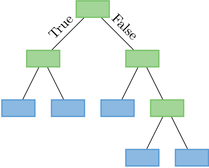
(a) Decision tree with a tree depth of 3. Green boxes: decision nodes with conditions on the input variables; blue boxes: leaves with output values.

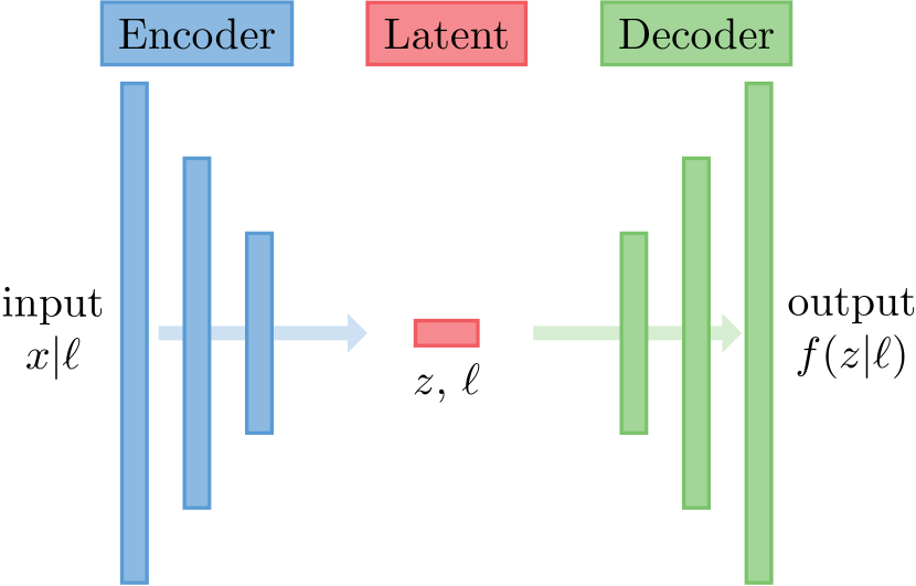
(b) CVAE architecture with input $x$, labels $\ell$, and latent space $z$.

Figure 7: Diagrams of ML algorithm architectures.

Although a conditional GAN using the infoGAN network architecture [49] was evaluated for this work, it did not perform as well as the CVAE because of difficulties related to the stability of training a multi-agent model, and results from this model are omitted for brevity.

3 Results

In this section, we present results of using the ML techniques to model the FPDF, $P(Z,c|\widetilde{Z},\widetilde{Z^{\prime\prime}},\widetilde{c},\widetilde{c^{\prime\prime}})$, from Equation (1). We first focus on using data from the volume centered at $z=0.1025\,\mathrm{m}$ because this section of the domain contains regions that are dominated by premixed burning of the fuel-air mixture from the nozzle and the burning of the products from the primary premixed flame mixing with the air from the co-flow, as discussed in Section 2.2. Next, we evaluate the generalization capabilities of the different algorithms by characterizing their performance on other sections of the flame.

We quantify model performance with two metrics of interest: the Jensen-Shannon divergence [50, 51] and the filtered progress variable source term. The Jensen-Shannon divergence measures the similarity between two PDFs and will characterize the error in predicting $P(Z,c|\widetilde{Z},\widetilde{Z^{\prime\prime}},\widetilde{c},\widetilde{c^{\prime\prime}})$. It is a symmetric version of the Kullback-Leibler divergence [52], and it is defined as:

$$J(Q||R)=\frac{1}{2}\left(D(Q||M)+D(R||M)\right)$$ (8)

where $D(Q||R)=\sum_{i=1}^{n}R(i)\ln{\left(\frac{R(i)}{Q(i)}\right)}$; $M=\nicefrac{{1}}{{2}}\left(Q+R\right)$; $Q$ and $R$ are PDFs of length $n$; and $0\leq J(Q||R)\leq\ln{(2)}$, with low values indicating more similarity between $Q$ and $R$. The Jensen-Shannon divergence exhibits several advantages over the Kullback-Leibler divergence: PDFs do not need to have the same support, it is symmetric, $J(Q||R)=J(R||Q)$, and it is bounded. The overall sub-filter PDF prediction accuracy of a model is characterized by the $90^{\text{th}}$ percentile of all the Jensen-Shannon divergences, denoted $J_{90}$. Examples of FDF modeling using the $\beta$-$\beta$ analytical model illustrate different Jensen-Shannon divergence values, Figure 8. This figure is similar to Figure 4, though it shows different realizations of $P(Z,c)$. The $\beta$-$\beta$ analytical model is not able to capture more complex FDF shapes, such as bimodal distributions, leading to high Jensen-Shannon divergence values, Figure 8(b), and it motivates the need for more accurate models. From these results, accurate predictions can be expected for $J(P||P_{m})<0.3$, whereas predictions with $J(P||P_{m})>0.6$ exhibit incorrect median values and overall shapes.

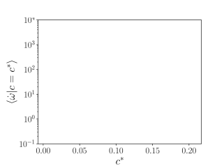
(a) $J(P||P_{\beta})=0$.

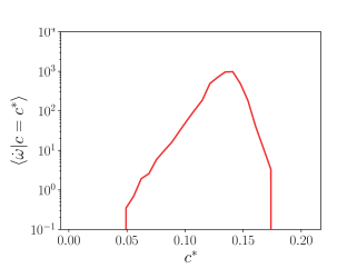
(b) $J(P||P_{\beta})=\nicefrac{{\ln{(2)}}}{{2}}$.

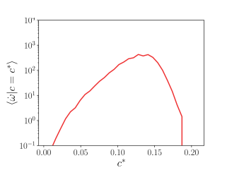
(c) $J(P||P_{\beta})=0.59$.

Figure 8: Marginal FDFs for low, mid-range, and high Jensen-Shannon divergence values for the $\beta$-$\beta$ PDF model. Red solid: RF; green dashed: DNN; blue dash-dotted: CVAE; orange short dashed: $\beta$-$\beta$ model; black solid: DNS.

The second metric of interest characterizes the error in predicting $\widetilde{\dot{\omega}}$ and is simply the normalized root mean square error (RMSE) of the model predictions, $\widetilde{\dot{\omega}}_{m}$:

$$\text{RMSE}(\widetilde{\dot{\omega}})=\frac{1}{\widetilde{\dot{\Omega}}}\sqrt{\frac{1}{|\mathcal{D}|}\sum_{i=1}^{|\mathcal{D}|}\left(\epsilon(\widetilde{\dot{\omega}}_{i})\right)^{2}},$$ (9)

where $\epsilon(\widetilde{\dot{\omega}}_{i})=\widetilde{\dot{\omega}}_{i}-\widetilde{\dot{\omega}}_{m,i}$ is the error, $\mathcal{D}$ is the data set over which the error is computed, and

$$\widetilde{\dot{\Omega}}=\sqrt{\frac{1}{|\mathcal{D}_{T}|}\sum_{i=1}^{|\mathcal{D}_{T}|}\left(\widetilde{\dot{\omega}}_{i}\right)^{2}}$$ (10)

is the normalization constant, and $\mathcal{D}_{T}=\bigcup\limits_{i=1,\dots,n_{v}}\mathcal{D}_{i}$. All metrics presented are computed with respect to the validation data sets.

3.1 Filtered density function predictions

ML models were trained using filtered DNS data from $\mathcal{V}_{3}$ (centered at $z=0.1025\,\mathrm{m}$), i.e., the algorithms were trained on $\mathcal{D}_{3}^{t}$, and the metrics were evaluated on $\mathcal{D}_{3}^{v}$. The random forests model training time for the 52920 FDFs in $\mathcal{D}_{3}^{t}$ was $1800\,\mathrm{s}$ on an Intel SandyBridge Xeon processor with $256\,\mathrm{GB}$ of memory. The DNN and CVAE training times were $2200\,\mathrm{s}$ and $3500\,\mathrm{s}$ on a NVIDIA Tesla K80 GPU. In addition to the ML models discussed in Section 2.4, we included an ordinary least squares regression (OLS) model as a baseline for additional discussion of the modeling results.

Several example FDF predictions are shown in Figure 8, corresponding to low, medium, and high values of $J(P||P_{\beta})$. The FDF and the cumulative density function for the Jensen-Shannon divergence of the predictions on the validation data, $J=J(P||P_{m})$, where $P_{m}$ is the modeled FDF, are presented in Figure 9. The three ML models exhibit similar FDF prediction errors with a narrow peak close to 0. The prediction error for the $\beta$-$\beta$ analytical model is larger than the prediction errors for the ML models; see Table 1. Additionally, comparing the training error, $J^{t}_{90}$, to the validation error, $J^{v}_{90}$, indicates that the random forests model overfits the training data (there is a large difference between the training and testing error), whereas the deep learning algorithms avoid overfitting; Table 1. Results from the OLS model, a low complexity model, exhibit $J^{t}_{90}$ and $J^{v}_{90}$ values that are approximately four times larger than that for the other ML models, Table 1. This indicates that the more complex ML models are capturing important complex physical effects that the OLS approach misses.

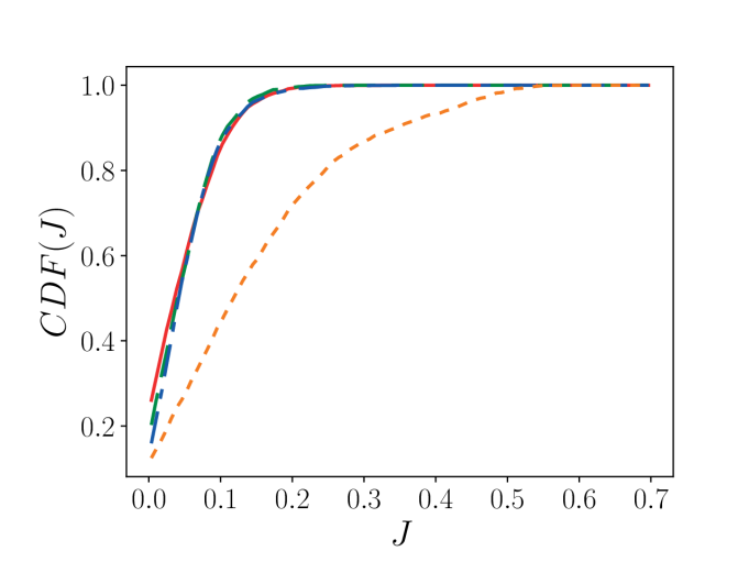
(a) FDF of $J$.

(b) Cumulative density function of $J$.

Figure 9: FDF predictions on validation data. Red solid: RF; green dashed: DNN; blue dash-dotted: CVAE; orange short dashed: $\beta$-$\beta$ model.

Model prediction times for each FDF were computed for all models as:

$$t_{m}=\frac{1}{n_{t}|\mathcal{D}_{3}^{v}|}\sum_{i=1}^{n_{t}}\text{time to evaluate }m(\mathcal{D}_{3}^{v})$$ (11)

where $n_{t}=10$ predictions on the validation data set $\mathcal{D}_{3}^{v}$, which contains 2940 samples, thereby necessitating 2940 model evaluations. Although the random forests model accuracy is similar to that of the neural networks, the model complexity required is such that the prediction time is approximately 20 times longer than the DNN and CVAE and the model size is more than 3000 times larger; see Table 1. The need for large amounts of memory for training and the slow prediction times illustrate the main drawback for the use of the random forests algorithm in production simulations from the standpoints of both training and prediction. Because the DNN and the CVAE decoder have similar architectures, their prediction time is similar. The $\beta$-$\beta$ model FPDF computations involve a discrete $\beta$ PDF evaluation in both $Z$ and $c$ and an outer product to compute the FPDF, leading to prediction times comparable with the random forests model. The $\beta$ PDF was computed through the SciPy library [53].

Model	$J^{t}_{90}$	$J^{v}_{90}$	$t_{m}\,(\mathrm{ms})$	RMSE $(\widetilde{\dot{\omega}})$	$R^{2}(\widetilde{\dot{\omega}})$	DoFs (million)	Memory (MB)
RF	0.03	0.12	0.932	0.22	0.97	5.2	82107
DNN	0.11	0.11	0.036	0.23	0.97	1.1	27
CVAE	0.11	0.12	0.038	0.22	0.97	2.3	36
$\beta$-$\beta$	0.35	0.35	1.178	0.63	0.75	–	–
OLS	0.43	0.43	0.018	0.69	0.70	0.008	0.1

Table 1: Summary of model performance and size for $P(Z,c|\widetilde{Z},\widetilde{Z^{\prime\prime}},\widetilde{c},\widetilde{c^{\prime\prime}})$ and $\widetilde{\dot{\omega}}$.

The FDF models were used to provide predictions of the reaction rate, $\widetilde{\dot{\omega}}$, by convoluting the predicted FDF with the reaction rate, Equation 1, where $\langle\dot{\omega}|Z,c\rangle$ is from the same $32^{3}$ box as that used to generate $P(Z,c|\widetilde{Z},\widetilde{Z^{\prime\prime}},\widetilde{c},\widetilde{c^{\prime\prime}})$. This ensures that the errors observed in the predictions of $\widetilde{\dot{\omega}}$ can be exclusively attributed to the FDF modeling. Table 1 and Figure 10 illustrate the different model performances in predicting $\widetilde{\dot{\omega}}$. The coefficient of determination, $R^{2}$, is above $0.95$ for the three discussed ML models, indicating a high model accuracy, whereas that of the $\beta$-$\beta$ model is significantly lower. The three different ML algorithms achieve similar results, Figure 10. The PDF of the error, $\epsilon(\widetilde{\dot{\omega}})$, as shown in Figure 10(b), is symmetric, indicating that the models are not biased toward under- or overpredicting. The $\beta$-$\beta$ analytical model has a broad range of prediction errors and tends to underpredict $\widetilde{\dot{\omega}}$ for $\widetilde{\dot{\omega}}>5$ in this volume, Figure 10(a). The OLS model presents an error that is three times larger than the other ML models and is slightly larger than the error of the $\beta$-$\beta$ model.

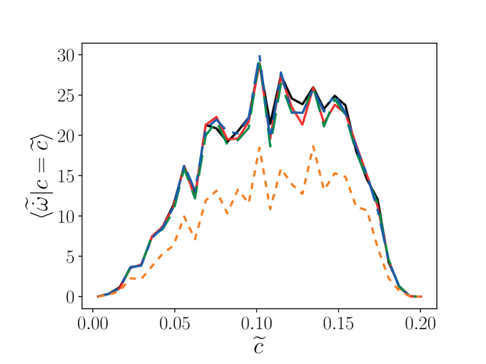
(a) $\widetilde{\dot{\omega}}$ predictions.

(b) PDF of $\epsilon(\widetilde{\dot{\omega}})$.

Figure 10: Reaction rate predictions. Red squares and solid: RF; green diamonds and dashed: DNN; blue circles and dash-dotted: CVAE; orange pentagons and short dashed: $\beta$-$\beta$ model.

3.2 Model generalization

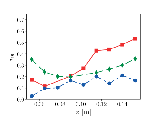
Figure 11: The $90^{\text{th}}$ percentile of $r_{i,j}$ as a function of height. Red squares and solid: $r_{3,j}$ for $j=1,\dots,n_{v}$; green diamonds and dashed: $r_{5,j}$ for $j=1,\dots,n_{v}$; blue circles and dash-dotted: $r_{i,j}$ for $i=[1,3,5,7,9]$ and $j=2,4,6,\,\text{and}\ 8$.

In this section, we examine the performance of the models trained using different data sets and their ability to generalize to data from other regions of the flame. An understanding of model generalization has important implications for the model’s applicability to other physical configurations. Because of the nature of the low-swirl burner flame, a wide range of different physical processes are encountered in different regions of the flame, and it is important to understand the conditions for a model’s applicability.

Three versions of the models were trained: (i) using $\mathcal{D}_{3}^{t}$ (volume centered at $z=0.0775\,\mathrm{m}$); (ii) using data from a volume farther downstream, $\mathcal{D}_{5}^{t}$ (volume centered at $z=0.1025\,\mathrm{m}$); and (iii) trained using data from every other volume $\mathcal{D}^{t}=\bigcup\limits_{i=1,3,5,7,9}\mathcal{D}_{i}^{t}$. Note that for the random forests trained on all volumes, the maximum depth size of the trees was reduced to 18 to avoid out-of-memory errors on a 256 GB node (the resulting model size exceeded 110 GB).

The difference between the FDFs in different volumes is quantified through the minimum of the pairwise Jensen-Shannon divergence between all FDFs belonging to $\mathcal{V}_{i}$ and all FDFs belonging to $\mathcal{V}_{j}$:

$$r_{i,j}=\min_{k=1,\dots,|\mathcal{D}_{i}^{v}|}J(P_{k}||P_{l})\quad\forall P_{k}\in\mathcal{D}_{i}^{v},\ \forall P_{l}\in\mathcal{D}_{j}^{v}.$$ (12)

Low values of $r_{i,j}$ indicate that $\forall P_{l}\in\mathcal{D}_{j}^{v}$ there is $P_{k}\in\mathcal{D}_{i}^{v}$, which has a small Jensen-Shannon divergence and, therefore, a similar shape. The $90^{\text{th}}$ percentile of $r_{i,j}$, $r_{90}$, for different data sets is presented in Figure 11. For $\mathcal{V}_{3}$, it is clear that the FDFs in regions of the flame that are farther downstream or upstream are significantly different; however, models trained using data from every other volume, $\mathcal{D}^{t}$, have training data that are representative of the entire simulation domain.

Figure 12 presents the predictions for the three different model versions. For models trained using data from only one volume, the FDF prediction error is lowest for that volume and increases as the model is used on downstream or upstream volumes. All three types of ML algorithms predict similar generalization error profiles. This indicates that these models, including the generative algorithm, are unable to extrapolate to non-proximate regions of the flame. This is consistent with the observation that the training data are not representative of the entire flow, Figure 11. The RMSE $(\widetilde{\dot{\omega}})$ decreases as a function of $z$ because the mean $\widetilde{\dot{\omega}}$ decreases as a function of $z$ as well. Models trained with $\mathcal{D}_{5}^{t}$ perform slightly better in the upstream portion of the domain, Figure 12(b), because the FDFs in $\mathcal{V}_{5}$ are more representative of the upstream FDFs, but fail to capture those where the premixed burning at the nozzle is dominant ($z\approx 0.05\,\mathrm{m}$), Figure 11.

Models trained using every other volume achieve errors that are approximately half the error of the $\beta$-$\beta$ analytical model, Figure 12(c). This indicates that the models are capable of interpolating the sample space across the entire physical domain while using only a small subsection of the samples in the domain. The ML models achieve very good accuracy and approximate the conditional means of $\widetilde{\dot{\omega}}$, which is the optimal estimator using these data, Figure 13. Significant overpredictions in the $\beta$-$\beta$ model are observed. These are driven by errors in upstream volumes, Figure 12(c), particularly at high $\widetilde{Z}$ and $\widetilde{c}$, Figure 13. Sample FDFs where $\widetilde{\dot{\omega}}>15$ are shown in Figure 14 for different Jensen-Shannon divergences computed on the DNN model. Bimodal distributions are accurately predicted by the ML models, and, even for the worse case, Figure 14(c), the shapes in $Z$ and $c$ are well modeled.

In addition to demonstrating the accuracy of the ML algorithms, these results illustrate that the $90^{\text{th}}$ percentile of $r_{i,j}$ is a good metric for characterizing FDF similarity and provides a model generalization criteria, $r_{90}<0.2$, for an a-priori assessment of model performance on new data. Models trained using a data set that has an $r_{90}<0.2$ with another data set will produce joint FDFs exhibiting $J_{90}<0.2$ and, consequently, accurate $\widetilde{\dot{\omega}}$ predictions. As a demonstration, a DNN model was trained using samples from the negative $x$-half of the volume $\mathcal{V}_{3}$ of the axisymmetric flame (centered at $x=y=0\,\mathrm{m}$), i.e., $\mathcal{D}^{t}=\{s~{}|~{}s\in\mathcal{D}_{3}^{t},~{}x_{s}<0\,\mathrm{m}\}$, and validated on predictions of samples in the positive $x$-half of the other volumes, $\mathcal{D}^{v}=\{s~{}|~{}s\in\mathcal{D}_{i}^{v},~{}x_{s}>0\,\mathrm{m},~{}i=1,\dots,n_{v}\}$. This model performs accurately on FDF predictions in nearby volumes, e.g., $J_{90}\approx 0.15$ in $\mathcal{V}_{2}$ and $\mathcal{V}_{3}$, and performs poorly at locations farthest downstream, e.g., $J_{90}=0.63$ in $\mathcal{V}_{7}$.

The last generalization test was performed by using data generated from a different time snapshot of the DNS ($t=0.059\,\mathrm{s}$) as that used to train the models. For this case, the DNN model trained on $\mathcal{D}^{t}=\bigcup\limits_{i=1,3,5,7,9}\mathcal{D}_{i}^{t}$ and the $\beta$-$\beta$ model were used to illustrate how these models perform on data from a different time instance of the DNS, Figure 15. The DNN model predicts similar $J_{90}$ values though they are slightly higher for the data from the time snapshot not used in the training. The $\beta$-$\beta$ model presents similar errors in both cases and these remain approximately three times higher than those of the DNN model. These generalization tests clearly demonstrate that the learned models are able to generalize temporally, as well as spatially.

The results in this section illustrate (i) the importance of using data representative of the extent of the physical processes present in the simulation and (ii) the potential to develop in situ ML modeling capabilities, where the model is developed during the simulation, without adversely affecting the simulation time because the most accurate models were trained using data from less than $4\%$ of the total DNS domain volume.

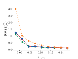
(a) $\mathcal{D}_{3}^{t}$ ($z_{3}=0.0775\,\mathrm{m}$).

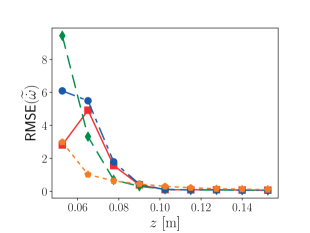
(b) $\mathcal{D}_{5}^{t}$ ($z_{5}=0.1025\,\mathrm{m}$).

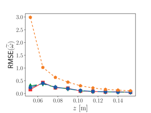
(c) $\mathcal{D}^{t}=\bigcup\limits_{i=1,3,5,7,9}\mathcal{D}_{i}^{t}$.

Figure 12: $J_{90}$ and RMSE $(\widetilde{\dot{\omega}})$ as a function of height using ML algorithms trained with data from different sections of the flame. Red squares and solid: RF; green diamonds and dashed: DNN; blue circles and dash-dotted: CVAE; orange pentagons and short dashed: $\beta$-$\beta$ model.

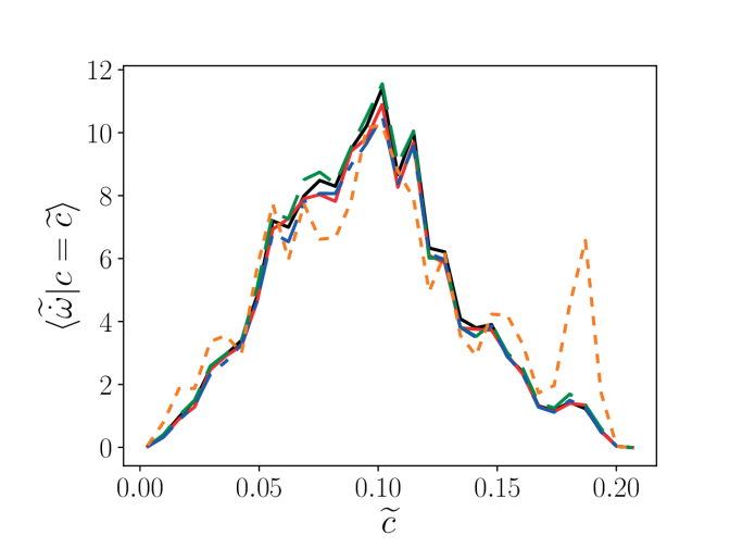
(a) $\widetilde{\dot{\omega}}$ predictions.

(b) Conditional means of $\widetilde{\dot{\omega}}$ as a function of $\widetilde{z}$.

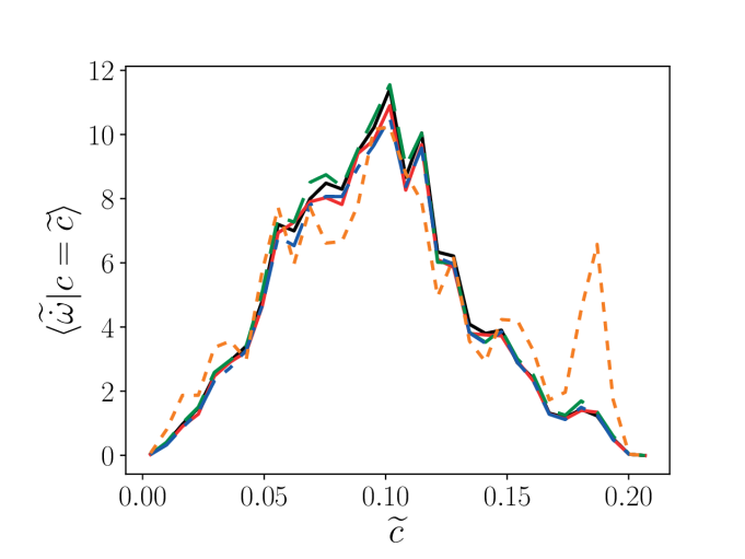
(c) Conditional means of $\widetilde{\dot{\omega}}$ as a function of $\widetilde{c}$.

Figure 13: Reaction rate predictions for models trained on $\mathcal{D}^{t}=\bigcup\limits_{i=1,3,5,7,9}\mathcal{D}_{i}^{t}$. Red squares and solid: RF; green diamonds and dashed: DNN; blue circles and dash-dotted: CVAE; orange pentagons and short dashed: $\beta$-$\beta$ model; black solid: DNS.

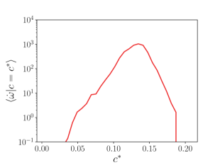
(a) $J(P||P_{\text{\lx@glossaries@gls@link{acronym}{dnn}{\leavevmode DNN}}})=0.05$.

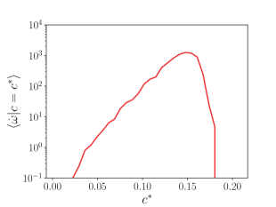
(b) $J(P||P_{\text{\lx@glossaries@gls@link{acronym}{dnn}{\leavevmode DNN}}})=0.1$.

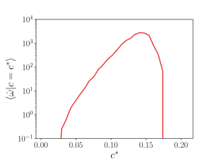
(c) $J(P||P_{\text{\lx@glossaries@gls@link{acronym}{dnn}{\leavevmode DNN}}})=0.21$.

Figure 14: Marginal FDFs for median and high Jensen-Shannon divergence values for models trained on $\mathcal{D}^{t}=\bigcup\limits_{i=1,3,5,7,9}\mathcal{D}_{i}^{t}$. Red solid: RF; green dashed: DNN; blue dash-dotted: CVAE; orange short dashed: $\beta$-$\beta$ model; black solid: DNS.

(a) $J_{90}$.

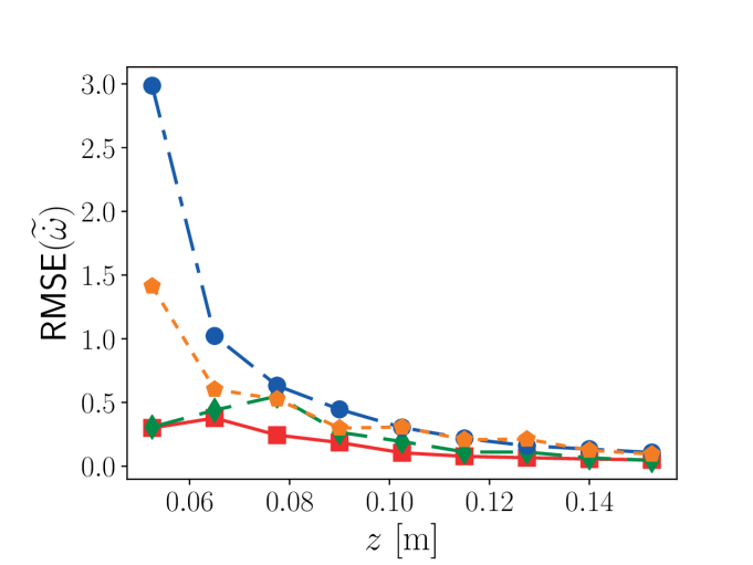
(b) RMSE $(\widetilde{\dot{\omega}})$.

Figure 15: $J_{90}$ and RMSE $(\widetilde{\dot{\omega}})$ as a function of height using the DNN model trained at $t=0.0626\,\mathrm{s}$ on $\mathcal{D}^{t}=\bigcup\limits_{i=1,3,5,7,9}\mathcal{D}_{i}^{t}$ and the $\beta$-$\beta$ model. Red squares and solid: DNN at $t=0.0626\,\mathrm{s}$; green diamonds and dashed: DNN at $t=0.059\,\mathrm{s}$; blue circles and dash-dotted: $\beta$-$\beta$ model at $t=0.0626\,\mathrm{s}$; orange pentagons and short dashed: $\beta$-$\beta$ model at $t=0.059\,\mathrm{s}$.

4 Conclusion

In this work, we used three different ML algorithms representative of different types of ML (traditional methods, deep learning, and generative learning) to design presumed PDF models for combustion applications. We showed that models designed through advanced ML techniques are better able to capture the complexity of these FDFs than analytical models or linear regression models. Although the random forests model predicts results similar to those of the deep learning models, this model is not suitable for in situ training and modeling because of the model complexity, which leads to high memory requirements and high prediction times. The deep learning algorithms were able to achieve the same high accuracy with fast prediction times and low model complexity. These models were also able to generalize to other spatial regions of the flame and to other time instances of the flame. In this study, generative learning models as used here, which present advantages in many deep learning applications through the use of a latent space representation, did not provide increased accuracy or better generalization characteristics compared to feed-forward neural networks. Additionally, the deep learning models provide fast predictions relative to the $\beta$-$\beta$ model, indicating that these methods might at the very least be efficient encoders of $\beta$-$\beta$ tabulation models by using DNS as a source of training data, resulting in encodings that provide more useful forms of the joint FDF not expressible by the $\beta$-$\beta$ model. Our results illustrate methodologies that can be successfully leveraged to derive accurate deep learning models for a wide range of applications. The results exhibited throughout this work indicate that deep learning models can be advantageously used for in situ modeling of turbulent combustion flows. These deep learning algorithms are readily integrated with scientific computing codes through PyTorch’s C++ API for future a-posteriori model evaluation. This work explores the construction of presumed PDF models parameterized by the commonly used four moments of the joint FDF using ML techniques. The existence of a unique FDF representation would require the specification of all the FDF moments. The lack of uniqueness is demonstrated in the results presented in this paper where a model constructed with a certain subset of the data failed to generalize to other regions of the flame. Addressing the non-uniqueness of the joint FPDFs will require the combustion community to explore modeling paradigms that do not solely rely on a finite set of FDF moments.

This work — including neural network models, analysis scripts, Jupyter notebooks, and figures — can be publicly accessed at the project’s GitHub page. Traditional ML algorithms were implemented through scikit-learn [27] and the deep learning algorithms through PyTorch [46].

References

Appendix A Summary of model parameters

The random forests model parameters are: number of estimators = 100, max. depth = 30, criterion is MSE, min. samples required to split node = 2, min. samples required for a leaf node = 1, max. number of features for best split = all, max. number of leaf nodes is unconstrained, bootstrapping when building trees is on, use out-of-bag samples to estimate the $R^{2}$ is off.

The DNN architecture is:

1. Linear layer (input features=4, output features=256, with bias)

2. LeakyReLU activation function with ($\alpha=0.01$)

3. BatchNorm1d (input and output features = 256, $\epsilon=10^{-5}$, decay of 0.1)

4. Linear layer (input features=256, output features=512, with bias)

5. LeakyReLU activation function with ($\alpha=0.01$)

6. BatchNorm1d (input and output features = 512, $\epsilon=10^{-5}$, decay of 0.1)

7. Linear layer (input features=512, output features=2048, with bias)

8. Softmax activation function

Additional DNN hyperparameters are: the learning rate ($10^{-4}$), the number of epochs (500), the batch size (64).

The CVAE encoder architecture and latent is:

1. Linear layer (input features=2052, output features=512, with bias)

2. ReLU activation function

3. Linear layer (input features=512, output features=256, with bias)

4. ReLU activation function

5. Latent space linear layer of means and variances (input features=256, output features=10, with bias)

The CVAE decoder architecture is:

1. Linear layer (input features=14, output features=256, with bias)

2. ReLU activation function

3. Linear layer (input features=256, output features=512, with bias)

4. ReLU activation function

5. Linear layer (input features=512, output features=2048, with bias)

6. Softmax activation function

Additional CVAE hyperparameters are: the learning rate ($10^{-3}$), the number of epochs (500), the batch size (64).

References

- Day et al. [2012] M. Day, S. Tachibana, J. Bell, M. Lijewski, V. Beckner, R. K. Cheng, A combined computational and experimental characterization of lean premixed turbulent low swirl laboratory flames, Combust. Flame 159 (1) (2012) 275–290, ISSN 00102180, doi:10.1016/j.combustflame.2011.06.016, URL http://linkinghub.elsevier.com/retrieve/pii/S0010218011001969.
- Cook and Riley [1994] A. W. Cook, J. J. Riley, A subgrid model for equilibrium chemistry in turbulent flows, Phys. Fluids 6 (8) (1994) 2868–2870, ISSN 1070-6631, doi:10.1063/1.868111, URL http://aip.scitation.org/doi/10.1063/1.868111.
- Jiménez et al. [1997] J. Jiménez, A. Liñán, M. M. Rogers, F. J. Higuera, A priori testing of subgrid models for chemically reacting non-premixed turbulent shear flows, J. Fluid Mech. ISSN 00221120, doi:10.1017/S0022112097006733.
- Bradley et al. [1998] D. Bradley, P. Gaskell, X. Gu, The mathematical modeling of liftoff and blowoff of turbulent non-premixed methane jet flames at high strain rates, Symp. Combust. 27 (1) (1998) 1199–1206, ISSN 00820784, doi:10.1016/S0082-0784(98)80523-7, URL https://linkinghub.elsevier.com/retrieve/pii/%****␣report.bbl␣Line␣50␣****S0082078498805237.
- Bradley et al. [2002] D. Bradley, D. Emerson, P. Gaskell, X. Gu, Mathematical modeling of turbulent non-premixed piloted-jet flames with local extinctions, Proc. Combust. Inst. 29 (2) (2002) 2155–2162, ISSN 15407489, doi:10.1016/S1540-7489(02)80262-0, URL https://linkinghub.elsevier.com/retrieve/pii/S1540748902802620.
- Ihme and Pitsch [2008a] M. Ihme, H. Pitsch, Prediction of extinction and reignition in nonpremixed turbulent flames using a flamelet/progress variable model: 1. A priori study and presumed PDF closure, Combust. Flame 155 (1-2) (2008a) 70–89, ISSN 00102180, doi:10.1016/j.combustflame.2008.04.001, URL https://linkinghub.elsevier.com/retrieve/pii/S0010218008000904.
- Ihme and Pitsch [2008b] M. Ihme, H. Pitsch, Prediction of extinction and reignition in nonpremixed turbulent flames using a flamelet/progress variable model: 2. Application in LES of Sandia flames D and E, Combust. Flame 155 (1-2) (2008b) 90–107, ISSN 00102180, doi:10.1016/j.combustflame.2008.04.015, URL https://linkinghub.elsevier.com/retrieve/pii/S0010218008001223.
- Fernández-Delgado et al. [2014] M. Fernández-Delgado, E. Cernadas, S. Barro, D. Amorim, D. Amorim Fernández-Delgado, Do we Need Hundreds of Classifiers to Solve Real World Classification Problems?, J. Mach. Learn. Res. ISSN 1532-4435, doi:10.1016/j.csda.2008.10.033.
- Liaw and Wiener [2002] A. Liaw, M. Wiener, Classification and Regression by randomForest, R news 2 (3) (2002) 18–22.
- Cybenko [1989] G. Cybenko, Approximation by superpositions of a sigmoidal function, Math. Control. Signals, Syst. 2 (4) (1989) 303–314, ISSN 0932-4194, doi:10.1007/BF02551274, URL http://link.springer.com/10.1007/BF02551274.
- Hornik [1991] K. Hornik, Approximation capabilities of multilayer feedforward networks, Neural Networks 4 (2) (1991) 251–257, ISSN 08936080, doi:10.1016/0893-6080(91)90009-T, URL http://linkinghub.elsevier.com/retrieve/pii/089360809190009T.
- Goodfellow et al. [2016] I. Goodfellow, Y. Bengio, A. Courville, Deep Learning, MIT Press, URL http://www.deeplearningbook.org, 2016.
- Veynante and Vervisch [2002] D. Veynante, L. Vervisch, Turbulent combustion modeling, Prog. Energy Combust. Sci. 28 (3) (2002) 193–266, ISSN 03601285, doi:10.1016/S0360-1285(01)00017-X, URL http://linkinghub.elsevier.com/retrieve/pii/S036012850100017X.
- Pitsch [2006] H. Pitsch, LARGE-EDDY SIMULATION OF TURBULENT COMBUSTION, Annu. Rev. Fluid Mech. 38 (1) (2006) 453–482, ISSN 0066-4189, doi:10.1146/annurev.fluid.38.050304.092133, URL http://www.annualreviews.org/doi/10.1146/annurev.fluid.38.050304.092133.
- van Oijen [2002] J. van Oijen, Flamelet-Generated Manifolds: Development and Application to Premixed Laminar Flames, Ph.D. thesis, Eindhoven University of Technology, Eindhoven, 2002.
- Gicquel et al. [2000] O. Gicquel, N. Darabiha, D. Thévenin, Liminar premixed hydrogen/air counterflow flame simulations using flame prolongation of ILDM with differential diffusion, Proc. Combust. Inst. 28 (2) (2000) 1901–1908, ISSN 15407489, doi:10.1016/S0082-0784(00)80594-9, URL http://linkinghub.elsevier.com/retrieve/pii/S0082078400805949.
- Klimenko and Bilger [1999] A. Y. Klimenko, R. W. Bilger, Conditional moment closure for turbulent combustion, Prog. Energy Combust. Sci. ISSN 03601285, doi:10.1016/S0360-1285(99)00006-4.
- Jin et al. [2008] B. Jin, R. Grout, W. K. Bushe, Conditional Source-Term Estimation as a Method for Chemical Closure in Premixed Turbulent Reacting Flow, Flow, Turbulence and Combustion 81 (4) (2008) 563–582, ISSN 1573-1987, doi:10.1007/s10494-008-9148-0, URL https://doi.org/10.1007/s10494-008-9148-0.
- Fox [2003] R. O. Fox, Computational Models for Turbulent Reacting Flows, Cambridge Univ. Press, Cambridge, UK, 2003.
- Grout et al. [2009] R. W. Grout, N. Swaminathan, R. S. Cant, Effects of compositional fluctuations on premixed flames, Combust. Theory Model. 13 (5) (2009) 823–852, ISSN 1364-7830, doi:10.1080/13647830903160291, URL http://www.tandfonline.com/doi/abs/10.1080/13647830903160291.
- Isaac et al. [2014] B. J. Isaac, A. Coussement, O. Gicquel, P. J. Smith, A. Parente, Reduced-order PCA models for chemical reacting flows, Combust. Flame 161 (11) (2014) 2785–2800, ISSN 00102180, doi:10.1016/j.combustflame.2014.05.011, URL https://linkinghub.elsevier.com/retrieve/pii/S0010218014001412.
- Linse et al. [2014] D. Linse, A. Kleemann, C. Hasse, Probability density function approach coupled with detailed chemical kinetics for the prediction of knock in turbocharged direct injection spark ignition engines, Combust. Flame 161 (4) (2014) 997–1014, ISSN 00102180, doi:10.1016/j.combustflame.2013.10.025, URL https://linkinghub.elsevier.com/retrieve/pii/S0010218013003994.
- Perry and Mueller [2018] B. A. Perry, M. E. Mueller, Joint probability density function models for multiscalar turbulent mixing, Combust. Flame 193 (2018) 344–362, ISSN 00102180, doi:10.1016/j.combustflame.2018.03.039, URL https://doi.org/10.1016/j.combustflame.2018.03.039https://linkinghub.elsevier.com/retrieve/pii/S0010218018301512.
- Cheng et al. [2000] R. Cheng, D. Yegian, M. Miyasato, G. Samuelsen, C. Benson, R. Pellizzari, P. Loftus, Scaling and development of low-swirl burners for low-emission furnaces and boilers, Proc. Combust. Inst. ISSN 15407489, doi:10.1016/S0082-0784(00)80344-6.
- Day and Bell [2000] M. S. Day, J. B. Bell, Numerical simulation of laminar reacting flows with complex chemistry, Combust. Theory Model. 4 (4) (2000) 535–556, ISSN 1364-7830, doi:10.1088/1364-7830/4/4/309, URL http://www.tandfonline.com/doi/abs/10.1088/1364-7830/4/4/309.
- Kazakov and Frenklach [1994] A. Kazakov, M. Frenklach, Reduced Reaction Sets based on GRI-Mech 1.2, URL http://www.me.berkeley.edu/drm/, 1994.
- Pedregosa et al. [2011] F. Pedregosa, G. Varoquaux, A. Gramfort, V. Michel, B. Thirion, O. Grisel, M. Blondel, P. Prettenhofer, R. Weiss, V. Dubourg, J. Vanderplas, A. Passos, D. Cournapeau, M. Brucher, M. Perrot, E. Duchesnay, Scikit-learn: Machine Learning in Python, J. Mach. Learn. Res. ISSN 1271-6669, doi:10.1007/s13398-014-0173-7.2.
- Breiman [2001] L. Breiman, Random forests, Mach. Learn. ISSN 08856125, doi:10.1023/A:1010933404324.
- Goodfellow et al. [2014] I. Goodfellow, J. Pouget-Abadie, M. Mirza, B. Xu, D. Warde-Farley, S. Ozair, A. Courville, Y. Bengio, Generative Adversarial Nets, Adv. Neural Inf. Process. Syst. 27 (2014) 2672–2680ISSN 10495258, doi:10.1017/CBO9781139058452, URL http://papers.nips.cc/paper/5423-generative-adversarial-nets.pdf.
- Burger et al. [2012] H. C. Burger, C. J. Schuler, S. Harmeling, Image denoising: Can plain neural networks compete with BM3D?, in: Proc. IEEE Comput. Soc. Conf. Comput. Vis. Pattern Recognit., ISBN 9781467312264, ISSN 10636919, 2392–2399, doi:10.1109/CVPR.2012.6247952, 2012.
- Dosovitskiy et al. [2015] A. Dosovitskiy, J. T. Springenberg, T. Brox, Learning to generate chairs with convolutional neural networks, in: Proc. IEEE Comput. Soc. Conf. Comput. Vis. Pattern Recognit., vol. 07-12-June, ISBN 9781467369640, ISSN 10636919, 1538–1546, doi:10.1109/CVPR.2015.7298761, 2015.
- Lefkimmiatis [2016] S. Lefkimmiatis, Non-Local Color Image Denoising with Convolutional Neural Networks, Proc. IEEE Conf. Comput. Vis. Pattern Recognit. (2016) 5882–5891doi:10.1109/CVPR.2017.623, URL http://arxiv.org/abs/1611.06757.
- Ledig et al. [2016] C. Ledig, L. Theis, F. Huszar, J. Caballero, A. Cunningham, A. Acosta, A. Aitken, A. Tejani, J. Totz, Z. Wang, W. Shi, Photo-Realistic Single Image Super-Resolution Using a Generative Adversarial Network, Conf. Comput. Vis. Pattern Recognit. (2016) 1–14ISSN 0018-5043, doi:10.1109/CVPR.2017.19, URL http://arxiv.org/abs/1609.04802.
- Tai et al. [2017] Y. Tai, J. Yang, X. Liu, Image super-resolution via deep recursive residual network, in: Proc. - 30th IEEE Conf. Comput. Vis. Pattern Recognition, CVPR 2017, vol. 2017-Janua, ISBN 9781538604571, 2790–2798, doi:10.1109/CVPR.2017.298, 2017.
- Lai et al. [2017] W. S. Lai, J. B. Huang, N. Ahuja, M. H. Yang, Deep laplacian pyramid networks for fast and accurate super-resolution, in: Proc. - 30th IEEE Conf. Comput. Vis. Pattern Recognition, CVPR 2017, vol. 2017-Janua, ISBN 9781538604571, ISSN 1063-6919, 5835–5843, doi:10.1109/CVPR.2017.618, 2017.
- Graves [2013] A. Graves, Generating sequences with recurrent neural networks. preprint, arXiv:1308.0850 ISSN 18792782, doi:10.1145/2661829.2661935.
- Wu et al. [2016] Y. Wu, M. Schuster, Z. Chen, Q. V. Le, M. Norouzi, W. Macherey, M. Krikun, Y. Cao, Q. Gao, K. Macherey, J. Klingner, A. Shah, M. Johnson, X. Liu, Ł. Kaiser, S. Gouws, Y. Kato, T. Kudo, H. Kazawa, K. Stevens, G. Kurian, N. Patil, W. Wang, C. Young, J. Smith, J. Riesa, A. Rudnick, O. Vinyals, G. Corrado, M. Hughes, J. Dean, Google’s Neural Machine Translation System: Bridging the Gap between Human and Machine Translation, ArXiv e-prints ISSN 1471003X, doi:10.1038/nrn2258.
- Kwon [2017] W. Kwon, Attention Is All You Need, arXiv1706.03762 [cs] .
- Silver et al. [2017] D. Silver, J. Schrittwieser, K. Simonyan, I. Antonoglou, A. Huang, A. Guez, T. Hubert, L. Baker, M. Lai, A. Bolton, Y. Chen, T. Lillicrap, F. Hui, L. Sifre, G. van den Driessche, T. Graepel, D. Hassabis, Mastering the game of Go without human knowledge, Nature 550 (7676) (2017) 354–359, ISSN 0028-0836, doi:10.1038/nature24270, URL http://www.nature.com/doifinder/10.1038/nature24270.
- Lecun et al. [2015] Y. Lecun, Y. Bengio, G. Hinton, Deep learning, Nature 521 (7553) (2015) 436–444, ISSN 14764687, doi:10.1038/nature14539.
- Schmidhuber [2015] J. Schmidhuber, Deep Learning in neural networks: An overview, Neural Networks 61 (2015) 85–117, ISSN 18792782, doi:10.1016/j.neunet.2014.09.003, URL http://dx.doi.org/10.1016/j.neunet.2014.09.003.
- Prieto et al. [2016] A. Prieto, B. Prieto, E. M. Ortigosa, E. Ros, F. Pelayo, J. Ortega, I. Rojas, Neural networks: An overview of early research, current frameworks and new challenges, Neurocomputing ISSN 18728286, doi:10.1016/j.neucom.2016.06.014.
- Liu et al. [2017] W. Liu, Z. Wang, X. Liu, N. Zeng, Y. Liu, F. E. Alsaadi, A survey of deep neural network architectures and their applications, Neurocomputing ISSN 18728286, doi:10.1016/j.neucom.2016.12.038.
- Ioffe and Szegedy [2015] S. Ioffe, C. Szegedy, Batch Normalization: Accelerating Deep Network Training by Reducing Internal Covariate Shift URL http://arxiv.org/abs/1502.03167.
- Kingma and Ba [2014] D. P. Kingma, J. Ba, Adam: A Method for Stochastic Optimization URL http://arxiv.org/abs/1412.6980.
- Paszke et al. [2017] A. Paszke, S. Gross, S. Chintala, G. Chanan, E. Yang, Z. DeVito, Z. Lin, A. Desmaison, L. Antiga, A. Lerer, Automatic differentiation in PyTorch, in: NIPS-W, 2017.
- Kingma and Welling [2013] D. P. Kingma, M. Welling, Auto-Encoding Variational Bayes URL http://arxiv.org/abs/1312.6114.
- Rezende et al. [2014] D. J. Rezende, S. Mohamed, D. Wierstra, Stochastic Backpropagation and Approximate Inference in Deep Generative Models URL http://arxiv.org/abs/1401.4082.
- Chen et al. [2016] X. Chen, Y. Duan, R. Houthooft, J. Schulman, I. Sutskever, P. Abbeel, InfoGAN: Interpretable Representation Learning by Information Maximizing Generative Adversarial Nets URL http://arxiv.org/abs/1606.03657.
- Endres and Schindelin [2003] D. M. Endres, J. E. Schindelin, A new metric for probability distributions, doi:10.1109/TIT.2003.813506, 2003.
- Österreicher and Vajda [2003] F. Österreicher, I. Vajda, A new class of metric divergences on probability spaces and its applicability in statistics, Ann. Inst. Stat. Math. ISSN 00203157, doi:10.1007/BF02517812.
- Kullback [1987] S. Kullback, Letters to the Editor, Am. Stat. 41 (4) (1987) 338–341, ISSN 0003-1305, doi:10.1080/00031305.1987.10475510, URL http://www.tandfonline.com/doi/abs/10.1080/00031305.1987.10475510.
- Jones et al. [01 ] E. Jones, T. Oliphant, P. Peterson, et al., SciPy: Open source scientific tools for Python, URL http://www.scipy.org/, [Online; accessed 12/10/2018], 2001–.