Localized surfaces of three dimensional topological insulators

Abstract

We study the surface of a three-dimensional spin chiral $\mathrm{Z}_{2}$ topological insulator (class CII), demonstrating the possibility of its localization. This arises through an interplay of interaction and statistically-symmetric disorder, that confines the gapless fermionic degrees of freedom to a network of one-dimensional helical domain-walls that can be localized. We identify two distinct regimes of this gapless insulating phase, a “clogged” regime wherein the network localization is induced by its junctions between otherwise metallic helical domain-walls, and a “fully localized” regime of localized domain-walls. The experimental signatures of these regimes are also discussed.

I Introduction

The surfaces of topological insulators (TIs) Hasan and Kane (2010); Qi and Zhang (2011); Chiu et al. (2016); Ludwig (2015) exhibit robust symmetry-protected metallic transport even in the presence of symmetry-preserving heterogeneity (disorder) as long as the bulk remains gapped. The evasion of Anderson localization Anderson (1958); Evers and Mirlin (2008) is due to the anomalous nature of the surface states, reflecting a nontrivial wavefunction topology of TI’s bulk. Characterization of such symmetry protected topological materials is a vibrant field of research in modern condensed matter physics Ando and Fu (2015); Mizushima et al. (2016).

Interactions can destabilize such metallic surfaces Vishwanath and Senthil (2013); Wang and Senthil (2013, 2014); Metlitski et al. (2014); Senthil (2015), gapping them out by either spontaneously breaking the protective symmetry, or inducing a symmetry-preserving topologically-ordered long-range entanglement. However, it has been noted Xu and Moore (2006); Wu et al. (2006) and explored more extensively by us Chou et al. (2018), that in a two-dimensional (2D) time-reversal symmetric $\mathrm{Z}_{2}$ TI (class AII) Kane and Mele (2005a, b); Bernevig and Zhang (2006) an interplay of interaction and disorder can lead to another possibility, namely to a glassy gapless but insulating edge. Such a localized state breaks the time-reversal symmetry spontaneously, but in “spin glass” fashion, preserving it statistically. It exhibits a localization length that is a non-monotonic function of disorder strength, and is best viewed as a localized insulator of half charge fermionic domain-walls (Luther-Emery Luther and Emery (1974) fermons) Chou et al. (2018). Such edge localization provides a potential explanation of the puzzling experimental observations in InAs/GaSb TI systems Du et al. (2015); Li et al. (2015); Du et al. (2017); Li et al. (2017a).

Figure 1: An illustration of a disordered interacting class CII TI surface, forming helical domain-walls (black solid curves), between topologically gapped green domains Morimoto et al. (2015a) and trivially gapped white regions. Zoom-in: The interdomain four-way junction modeled as two helical Luttinger liquids with an impurity (junction) perturbation.

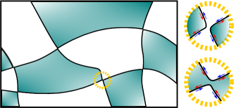
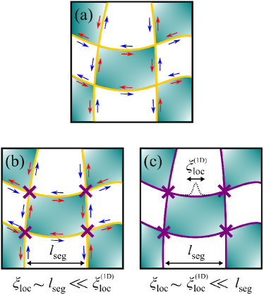
Motivated by this nontrivial disorder-interaction interplay in an edge of a 2D TI, we explore such phenomena in a 2D surface of a three-dimensional (3D) TI and find that only the CII class realizes this idea, namely, exhibits a gapless localized surface. We thus focus on the CII class TIs in the presence of symmetry breaking, but statistically preserving disorder. Such a disorder potential can in principle be generated dynamically Morimoto et al. (2015b); Song and Schnyder (2017). It allows for three distinct possibilities: a network of chiral (particle-hole symmetric) or helical (time-reversal symmetric) domain-walls Potter et al. (2017) (see Fig. 1), or a fully gapped (time-reversal and particle-hole symmetry-broken) insulators, depending on which symmetries are broken by disorder. As we demonstrate below, for the second case of a network of helical domain-walls, in the presence of interactions, a CII class TI surface indeed displays a phase transition to a gapless insulating surface. The latter exhibits two regimes: a “clogged” regime in which the barriers to transport are the junctions in the network of otherwise delocalized domain-walls Teo and Kane (2009), and a fully localized regime of interpenetrating one-dimensional (1D) localized helical edge states Chou et al. (2018). These interaction-induced regimes are obtained via standard analysis for helical Luttinger liquids Wu et al. (2006); Xu and Moore (2006); Chou et al. (2018); Teo and Kane (2009). Topological insulators in other symmetry classes of the ten-fold way do not allow this novel possibility.

The article is organized as follows. We begin in Sec. II with an introduction of a continuum model of a surface of CII class TI. We discuss three classes of symmetry-breaking heterogeneities that preserve its statistical symmetry in Sec. III, focusing on the helical network surface. A single interacting helical junction is studied in Sec. IV.2, and is utilized to make arguments for a localization transition in the helical surface network. We conclude with experimental signatures and the future directions in Sec. V.

II Surface Model

Three dimensional TIs are characterized by symmetry-protected metallic surfaces that host 2D massless Dirac or Majorana quasiparticles Schnyder et al. (2008); Hasan and Kane (2010); Qi and Zhang (2011). In the absence of interaction, they are robust to gapping out or localization by any symmetry-preserving single particle scattering. We focus on the spin chiral TI (class CII) Schnyder et al. (2008); Hosur et al. (2010), characterized by a $\mathrm{Z}_{2}$ invariant. Its topologically nontrivial surface exhibits two-valley Dirac cones with the chemical potential pinned to the Dirac point. The corresponding noninteracting clean CII surface Hamiltonian is given by

$$H_{0}= v_{D}\int\limits_{\bm{\mathrm{x}}}\Psi^{\dagger}\left[-i\hat{\sigma}^{x}\partial_{x}-i\hat{\sigma}^{y}\partial_{y}\right]\Psi,$$ (1)

where $\Psi$ is a four component fermionic Dirac field and $\hat{\sigma}^{x,y,z}$ is the “spin” Pauli matrix.

The clean surface Hamiltonian, $H_{0}$ can be perturbed by a number of fermion bilinear operators, $\Psi^{\dagger}\hat{T}_{a}\Psi$ (listed in Table 1), that can be classified by their commutation/anticommutation with $\hat{\sigma}^{x}$ and $\hat{\sigma}^{y}$ ( $[\hat{T}_{a},\hat{\sigma}^{x}]$, $[\hat{T}_{a},\hat{\sigma}^{y}]$, $\{\hat{T}_{a},\hat{\sigma}^{x}\}$, and $\{\hat{T}_{a},\hat{\sigma}^{y}\}$). If a bilinear commutes with both the $\hat{\sigma}^{x}$ and $\hat{\sigma}^{y}$, it is regarded as a scalar operator, denoted by $\hat{V}_{a}$. A vector operator, $\hat{A}_{a}$, commutes with one of the $\hat{\sigma}^{x}$ or $\hat{\sigma}^{y}$, but anticommutes with the other one. The mass operator, $\hat{M}_{a}$, anticommutes with both the $\hat{\sigma}^{x}$ and $\hat{\sigma}^{y}$.

We first focus on the symmetric bilinear operators given by

$$H_{\text{dis}}= \int\limits_{\bm{\mathrm{x}}}\Psi^{\dagger}\left[v_{1}\hat{\tau}^{x}+v_{2}\hat{\tau}^{z}+a_{1}\hat{\sigma}^{x}\hat{\tau}^{y}+a_{2}\hat{\sigma}^{y}\hat{\tau}^{y}\right]\Psi,$$ (2)

where $\hat{\tau}^{x,y,z}$ is the “valley” Pauli matrix. The bilinear operators $v_{1}({\bf x})$, $v_{2}({\bf x})$ are scalar and $a_{1}({\bf x})$, $a_{2}({\bf x})$ vector, time- and particle-hole symmetry-preserving random potentials. The time reversal ($\mathcal{T}$) and the particle-hole ($\mathcal{P}$) operations are defined by

$$\mathcal{T}:\Psi\rightarrow i\hat{\sigma}^{y}\Psi,\,\,\,i\rightarrow-i,$$ (3a)

$$\mathcal{P}:\Psi\rightarrow \hat{\sigma}^{x}\hat{\tau}^{y}(\Psi^{\dagger})^{T}.$$ (3b)

We note that the matrices in both symmetry operations ($\hat{\sigma}^{y}$ and $\hat{\sigma}^{x}\hat{\tau}^{y}$) are antisymmetric because they correspond to $\mathcal{T}^{2}=-1$ and $\mathcal{P}^{2}=-1$ Chiu et al. (2016); Ludwig (2015). In addition, a chiral operation ($\mathcal{S}=\mathcal{T}\mathcal{P}$) can be defined as a product of $\mathcal{T}$ and $\mathcal{P}$. All the bilinear operators in Table 1 are classified by these symmetries as well.

We now consider symmetry-breaking random bilinear perturbations to the $\mathcal{T}$, $\mathcal{P}$ symmetric CII surfaces. Although (as listed in Table 1) there are various scalar $(\hat{V}_{a})$ and vector $(\hat{A}_{a})$ operators, these do not open up a gap or induce a localization, unlike the mass operator $\hat{M}_{a}$ Ludwig et al. (1994); Morimoto et al. (2015a). We thus focus on random symmetry-breaking masses, $H_{\text{M}}=\sum_{a=1}^{4}H_{\text{M},a}$, with

$$H_{\text{M},a}=\int\limits_{\bf x}m_{a}({\bf x})\Psi^{\dagger}\hat{M}_{a}\Psi.$$ (4)

These can be classified as follows (also in Table 1): $\hat{M}_{1}=\hat{\sigma}^{z}$ preserves $\mathcal{P}$ but breaks $\mathcal{T}$; $\hat{M}_{2}=\hat{\sigma}^{z}\hat{\tau}^{y}$ preserves $\mathcal{T}$ but breaks $\mathcal{P}$; $\hat{M}_{3}=\hat{\sigma}^{z}\hat{\tau}^{x}$ and $\hat{M}_{4}=\hat{\sigma}^{z}\hat{\tau}^{z}$ preserve $\mathcal{S}=\mathcal{T}\mathcal{P}$ but break both $\mathcal{T}$ and $\mathcal{P}$.

For our purposes here, we imagine simply imposing the random sign-changing amplitudes, $m_{a}(\bm{\mathrm{x}})$, such that statistically (averaged over disorder or samples) $\mathcal{T},\mathcal{P}$ symmetries remain intact, i.e., $m_{a}$ has zero mean. More physically, such random mass operators can arise as a result of heterogeneous spontaneous symmetry breaking in the presence of symmetric quenched disorder $H_{\text{dis}}$ and four-Fermi interactions

$$H_{I}=\sum_{a=1}^{4}U_{a}\int\limits_{\bm{\mathrm{x}}}\left[\Psi^{\dagger}\hat{M}_{a}\Psi\right]^{2},$$ (5)

where $U_{a}$ denotes the interaction strength corresponding to the mass $\hat{M}_{a}$ Morimoto et al. (2015b); Song and Schnyder (2017), with $m_{a}(\bm{\mathrm{x}})$ the mean-field order parameter determined self-consistently Morimoto et al. (2015b).

$\hat{T}_{a}$	Billinear operator	$\mathcal{T}$	$\mathcal{P}$	$\mathcal{S}$	Class
$\hat{V}_{1,2}$	$\hat{\tau}^{x}$, $\hat{\tau}^{z}$	$\checkmark$	$\checkmark$	$\checkmark$	CII
$\hat{A}_{1,2}$	$\hat{\sigma}^{x}\hat{\tau}^{y}$, $\hat{\sigma}^{y}\hat{\tau}^{y}$	$\checkmark$	$\checkmark$	$\checkmark$	CII
$\hat{V}_{3}$	$\hat{\tau}^{y}$	$\mathsf{x}$	$\checkmark$	$\mathsf{x}$	C
$\hat{A}_{3,4,5,6}$	$\hat{\sigma}^{x}\hat{\tau}^{x}$, $\hat{\sigma}^{x}\hat{\tau}^{z}$, $\hat{\sigma}^{y}\hat{\tau}^{x}$, $\hat{\sigma}^{y}\hat{\tau}^{z}$	$\mathsf{x}$	$\checkmark$	$\mathsf{x}$	C
$\hat{M}_{1}$	$\hat{\sigma}^{z}$	$\mathsf{x}$	$\checkmark$	$\mathsf{x}$	C
$\hat{V}_{4}$	$\hat{1}$	$\checkmark$	$\mathsf{x}$	$\mathsf{x}$	AII
$\hat{M}_{2}$	$\hat{\sigma}^{z}\hat{\tau}^{y}$	$\checkmark$	$\mathsf{x}$	$\mathsf{x}$	AII
$\hat{A}_{7,8}$	$\hat{\sigma}^{x}$, $\hat{\sigma}^{y}$	$\mathsf{x}$	$\mathsf{x}$	$\checkmark$	AIII
$\hat{M}_{3,4}$	$\hat{\sigma}^{z}\hat{\tau}^{x}$, $\hat{\sigma}^{z}\hat{\tau}^{z}$	$\mathsf{x}$	$\mathsf{x}$	$\checkmark$	AIII

Table 1: Classification of the bilinear operators in terms of the time-reversal ($\mathcal{T}$), particle-hole ($\mathcal{P}$), and chiral ($\mathcal{S}=\mathcal{T}\mathcal{P}$) operations on the CII class [as defined in Eq. (3)], and the type of perturbations ($\hat{V}_{a}$, $\hat{A}_{a}$, and $\hat{M}_{a}$).

Independent of the physical mechanism, we expect the CII symmetry-breaking random perturbation $H_{\text{M}}$ to generate a surface ground state that is a network of 1D domain walls, similar to statistical topological insulators Fulga et al. (2014); Morimoto et al. (2015a), illustrated in Fig. 1, the fate of which, in the presence of interactions is the focus of our work.

III CII class symmetry-broken surface states

In a three-dimensional CII class TI, the random symmetry-breaking mass operators $\hat{M}_{a}$ can lead to three types of domain-wall networks, corresponding to three distinct symmetries of sign-changing masses $m_{a}({\bf x})$ introduced in Sec. II (see Table 1). As we will discuss below, with one type of a mass, the inhomogeneous symmetry breaking leads to a surface state composed of a network of gapless 1D domain-walls separating domains characterized by a positive and negative value of a mass $m_{a}$. In the CII class, it is also possible to generate multiple mass terms when only the chiral symmetry ($\mathcal{S}$) is preserved. In this case the symmetry-breaking order parameter is a vector, that can rotate smoothly without vanishing, and as a result, such surface state, previously discussed Vishwanath and Senthil (2013); Wang and Senthil (2013, 2014); Metlitski et al. (2014); Senthil (2015), is fully gapped. Looking for a new, gapless but localized TI surface scenario, here we instead focus on the case only time-reversal ($\mathcal{T}$) or particle-hole ($\mathcal{P}$) symmetry is unbroken, such that there are sharp gapless domain-walls, that we will argue can get localized for the case of $\hat{M}_{2}$ disorder in the presence of interactions.

The transport in such symmetry-broken surface states of CII TIs is governed by the resulting network of the massless 1D domain-walls. The domain-wall surface states can be derived analytically in the large domain size limit via the standard “twist mass” formalism Jackiw and Rebbi (1976); Su et al. (1979). The 1D nature of the domain-walls is interrupted by regions where two domain walls come close to each other. These can be modeled as junctions illustrated in Fig. 1.

Here we are outlining the underlying physics and the approach, relegating the technical analysis to the Appendices. To make progress, we take the effect due to the random mass symmetry-breaking operators [given by Eq. (4)] to be much stronger than the symmetric disorder [given by $H_{\text{dis}}$ in Eq. (1)]. Therefore, we first compute the zero energy states of $H_{0}+H_{\text{M},a}$, determining the structure of the 1D electron domain-walls. We find that only one class, the helical domain-walls, arising by domains breaking $\mathcal{P}$ but not $\mathcal{T}$ symmetry, have the possibility of localization. We then study the stability of the resulting network to interactions and symmetric disorder, $H_{\text{dis}}$, taking advantage of our earlier work on 1D edges of 2D TIs Chou et al. (2018), as well as the analysis of the four-way junctions Teo and Kane (2009). The other symmetry-breaking scenarios are robust to symmetric disorder and interactions and thus such disordered TI surfaces remain metallic.

III.1 Particle-hole symmetric surface: Chiral domain-wall network

A particle-hole symmetric but time-reversal broken surface corresponds to the random mass operator $\hat{M}_{1}=\hat{\sigma}^{z}$. In this case the 1D domain-walls are chiral with two co-moving electrons. The chiral domain-wall states can be viewed as the spin quantum Hall edge of class C Gruzberg et al. (1997); Senthil et al. (1998); Gruzberg et al. (1999); Senthil et al. (1999). The intersections or proximity of chiral domain-walls can only rearrange their connectivity, but cannot stop the network state from conducting. Such a metallic state can be realized as a statistical topological insulator Fulga et al. (2014); Morimoto et al. (2015a), or, alternatively can be viewed as a critical state at the plateau transition Evers and Mirlin (2008). These are well known to be robust against local symmetric disorder perturbations, as with conventional quantum Hall states. We are not aware of any new physics to be discovered here from the interplay of disorder and interactions, at least in the large domain size limit, where the domain-wall structure can be derived analytically.

III.2 Time-reversal symmetric surface: Helical domain-wall network

Figure 2: Three possible regimes in the helical domain-wall networks. (a) Metallic regime. The helical network remains conducting for weaker Luttinger liquid interaction, $K>1/2$. (b) “Clogged” regime. For $3/8<K\leq 1/2$, the symmetric disorder remains irrelevant, but the random junctions (intersections) of the helical domain-walls are relevant and therefore block the dc transport, with helical electrons confined in the inter-junction domain-wall segments, breaking time-reversal symmetry spontaneously Teo and Kane (2009). A clogged state also persists for $K<3/8$ when the 1D domain-wall localization length ($\xi_{\text{loc}}^{(\text{1D})}$) is much longer than the typical length of the domain-wall segment ($l_{\text{seg}}$). As indicated in the figure, in the clogged regime, the true physical localization length, $\xi_{\text{loc}}$ is set by $l_{\text{seg}}$. (c) “Fully-localized” regime. For $K\leq 3/8$ and sufficiently small 1D domain-wall localization length ($\xi_{\text{loc}}^{(\text{1D})}\ll l_{\text{seg}}$), the whole domain-wall network becomes localized with a localization length set by $\xi_{\text{loc}}^{(\text{1D})}$. The yellow (purple) solid lines indicate the conducting (localized) channels; the purple crosses mark the perfect barrier junctions; the blue and red arrows indicate the movement of the domain-wall electrons that form Kramers pairs in each domain-wall segment.

We now turn to the most interesting case with a time-reversal symmetric surface, but with particle-hole symmetry randomly broken by the mass operator $\hat{M}_{2}=\hat{\sigma}^{z}\hat{\tau}^{y}$. In this case, the domain-walls form a helical network state Potter et al. (2017), protected against localization in the absence of interactions Kane and Mele (2005a); Xie et al. (2016), and have been studied previously Obuse et al. (2007, 2008); Ryu et al. (2010); Obuse et al. (2014). We emphasize that class CII TI is the only ten-fold way insulator that realizes a network of helical states under inhomogeneous symmetry breaking. The surface remains metallic as long as the time-reversal symmetry is intact. We next discuss the stability of this metallic helical network to interactions and symmetry-preserving disorder in the remainder of this subsection, with the technical analysis presented in Sec. IV.2.

Such surface transport is governed by the network of interacting helical domain-walls. At length scales shorter than the distance between junctions the physics is controlled by isolated helical domain walls, analyzable as a helical Luttinger liquid Wu et al. (2006); Xu and Moore (2006). For sufficiently strong repulsive interactions, $K<3/8$, these can be localized Wu et al. (2006); Xu and Moore (2006); Chou et al. (2018) due to an interplay of symmetric disorder and umklapp four-fermion interaction Chou et al. (2018). Such a localized state spontaneously and inhomogeneously breaks the time-reversal symmetry and is best viewed by a localized insulator of $e/2$-charge Luther-Emery fermions Chou et al. (2018). Thus for $K<3/8$, such TI surface becomes a network of localized one-dimensional insulators. This picture is self-consistent as long as the localization length along the one-dimensional domain-walls is short compared to the typical distance between junctions of the network, a condition that can be satisfied by taking the domains to be sufficiently large.

In the complementary regime of weaker interactions, $K>3/8$, the isolated 1D domain-wall segments are not localized, requiring an analysis of the full network, controlled by domain-walls proximity (intersections), that we model as four-way junctions. The latter problem is related to the earlier studies of the corner junction Hou et al. (2009) and the point contact Teo and Kane (2009). We perform a complementary analysis based on two helical Luttinger liquids with symmetry-allowed impurity perturbations in Sec. IV.2 and Appendix B. As we will demonstrate, for sufficiently strong interactions, $K<1/2$, the junctions become strong impurity barriers that suppress all conduction (before, i.e., for weaker interaction than localization of isolated domain-walls, $K<3/8$ Wu et al. (2006); Xu and Moore (2006); Chou et al. (2018)), and break the time-reversal symmetry spontaneously. Our results are consistent with the earlier finding in the helical liquid point contact study with spin-orbit couplings Teo and Kane (2009).

Combining the results from both the junction and the domain-wall states, we conclude the existence of three regimes (summarized in Fig. 2) in the large domains limit. For weak interactions $(K>1/2)$, the helical network remains conducting and can be viewed as a statistical TI surface Fulga et al. (2014); Morimoto et al. (2015a). For intermediate interactions $(3/8<K\leq 1/2)$, the junctions break time-reversal symmetry spontaneously and suppress the conduction. The domain-wall state in each segment remains “delocalized”, but the junctions block transport. We refer to this as a “clogged” regime. For sufficiently strong interactions $(K\leq 3/8)$, all the junctions and the domain-wall segments break time-reversal symmetry spontaneously and form a network of localized one-dimensional channels. Because the “clogged” and “fully localized” states are qualitatively the same, they are two distinct regimes connected by a smooth crossover (driven by interaction strength $K$) within a single insulating phase that sets in for $K<1/2$. We discuss this crossover further in Sec. IV.2.

III.3 Surface with only chiral symmetry: Gapped insulator

Lastly, for completeness, we discuss the CII TI surface with both time-reversal and particle-hole symmetry broken by two mass operators, $\hat{M}_{3}=\hat{\sigma}^{z}\hat{\tau}^{x}$ and $\hat{M}_{4}=\hat{\sigma}^{z}\hat{\tau}^{z}$, corresponding to the chiral symmetric class AIII. Qualitatively distinct from the case of a single mass, such symmetry broken surface state is typically fully gapped because the domains with multiple masses can deform from one to another without closing the gap Morimoto et al. (2015a), a possibility that was anticipated in the previous studies Vishwanath and Senthil (2013); Wang and Senthil (2013, 2014); Metlitski et al. (2014); Senthil (2015). Thus, such a surface is a fully gapped insulator up to disorder-induced rare in-gap states.

Finally we note that for a fine-tuned microscopic model, where only one type of bilinear appears, e.g., $\hat{M}_{3}=\hat{\sigma}^{z}\hat{\tau}^{x}$ or $\hat{M}_{4}=\hat{\sigma}^{z}\hat{\tau}^{z}$, a domain-wall network can be realized. However, the domain-walls of this network carry conventional one dimensional electrons. They thus do not enjoy the protection of $\mathcal{T}$ symmetry against localization and can therefore be Anderson-localized by disorder alone, in the absence of interactions.

IV Helical domain-network analysis

We now focus on a helical domain-wall network and analyze its stability to interactions and symmetry-preserving disorder. To this end, we first demonstrate localization along independent 1D domain-walls, and then show that the localization is stable to the ever-present domain-wall junctions, whose effect is to enhance localization by shifting the critical point to weaker interactions.

IV.1 Independent helical domain-walls

At short length scales (shorter than the typical inter-junction separation) we can neglect the domain-wall junctions and focus on the nature of individual helical domain-wall segments. In this limit, the problem reduces to independent 1D helical conductors, in the presence of symmetry-preserving disorder and interactions. This problem is technically identical to that of an interacting disordered edge of a 2D TI in the AII class Wu et al. (2006); Xu and Moore (2006); Chou et al. (2018), that can be localized by the interplay of symmetric disorder and interactions.

To see this, we consider a helical conductor modeled as counter-propagating states of right $(R)$ and left ($L$) moving helical fermions, with the low-energy disorder-free Hamiltonian given by

$$H_{\text{hLL}}=v_{F}\int\limits_{x}\left[R^{\dagger}\left(-i\partial_{x}R\right)-L^{\dagger}\left(-i\partial_{x}L\right)\right]+H_{\text{int}},$$ (6)

where $v_{F}$ is the Fermi velocity and $H_{\text{int}}$ encodes the Luttinger liquid interactions Giamarchi (2004); Shankar (2017). Although $H_{\text{hLL}}$ takes the same form as the spinless Luttinger liquid Giamarchi (2004); Shankar (2017), it is distinct from it, as in the helical Luttinger liquids the time-reversal symmetry ($R\rightarrow L$, $L\rightarrow-R$, and $i\rightarrow-i$) satisfies $\mathcal{T}^{2}=-1$, and thereby forbids single-particle backscattering perturbation, $L^{\dagger}R$.

Thus symmetric disorder only allows forward scattering,

$$H_{\text{chem}}=\int\limits_{x}V(x)\left(R^{\dagger}R+L^{\dagger}L\right),$$ (7)

that in the absence of additional interactions does not lead to localization.

The helical Luttinger liquid is also generically stable to the (disorder-free) time-reversal symmetric two-particle umklapp scattering,

$$H_{\text{umklapp}}=\int\limits_{x}\left[e^{i(4k_{F}-Q)x}:(L^{\dagger}R)^{2}:+\text{H.c.}\right]$$ (8)

($:A:$ is the normal ordering of $A$) as long the reciprocal lattice wavevector $Q$ is sufficiently incommensurate, i.e., as long as $|4k_{F}-Q|>\delta Q_{c}$ ($\delta Q_{c}$ the critical threshold) is satisfied Pokrovsky and Talapov (1979).

However, in the presence of symmetric disorder, that statistically makes up the wavevector incommensuration, the umklapp interaction generates a random time-reversal symmetric two-fermion back-scattering, that can lead to a localization of the 1D helical Luttinger liquid and the associated spin-glass-like time-reversal symmetry breaking Chou et al. (2018). Indeed, the standard renormalization group (RG) analysis shows that an interacting disordered helical conductor can be localized for $K<3/8$ Wu et al. (2006); Xu and Moore (2006). Alternatively, the problem at $K=1/4$ can be mapped onto noninteracting Luther-Emery fermions Luther and Emery (1974) with chemical potential disorder Chou et al. (2018), a model that is known to give localization for the entire spectrum Bocquet (1999). Such an interacting localized state is best viewed as an Anderson localized insulator of half-charge fermions (solitons), that exhibits a nonmonotonic localization as a function of disorder strength Chou et al. (2018).

Such localization of the 1D helical liquids then directly predicts a localization of long segments of nonintersecting domain-wall, valid in the regime when domain-wall junctions can be neglected. We next analyze the complementary regime where junctions play an essential role in localization of the CII surface.

IV.2 Interacting helical junction

For a weaker electron interaction $K>3/8$ and/or smaller domain size, the domain-wall intersections become important, and it is necessary to take into account junctions (see zoom-in of Fig. 1). At the technical level, the problem of the four-way helical junction is related to the studies of a corner junction Hou et al. (2009) and point contact Teo and Kane (2009) in a 2D topological insulator. In these previous works, the junction of four semi-infinite helical Luttinger liquids is mapped to an infinite spinful Luttinger liquid with an impurity interaction. We present a technically distinct but physically equivalent analysis based on two isolated Luttinger liquids with junction perturbations.

We thus consider two 1D generic helical Luttinger liquids $+,-$, interacting via a local junction perturbation, corresponding to two helical domain-walls coming to close proximity (see the zoom-in in Fig. 1). Because these are boundaries of the same type of gapped domains, they map onto two 1D Luttinger liquids of opposite helicity, described by two copies of the helical Hamiltonian [Eq. (6)],

$$H_{\text{hLL},2}= v_{F}\sum_{s=\pm}\int\limits_{x}\left[R_{s}^{\dagger}\left(-i\partial_{x}R_{s}\right)-L_{s}^{\dagger}\left(-i\partial_{x}L_{s}\right)\right]+H_{\text{int},2},$$ (9)

where $R_{s}$ ($L_{s}$) is the right (left) moving fermion, with the index $s$ labeling the two helical domain-walls and $H_{\text{int},2}$ encoding the Luttinger liquid interactions Giamarchi (2004) within each helical liquid. For simplicity, we take these two to have the same Fermi velocity ($v_{F}$) and Luttinger liquid interaction; we expect our qualitative conclusions to remain valid away from this special case.

To construct junction perturbations, we enumerate all bilinear and quartic operators allowed by the time-reversal symmetry Tanaka and Nagaosa (2009); Chou et al. (2015). For example, as usual the single-particle backscattering within the same helical liquid ($L^{\dagger}_{s}R_{s}$) is forbidden. We will also ignore perturbations that are always irrelevant in the RG analysis. The single particle forward and backward tunneling processes between the two helical liquids are given by

$$H_{\text{junc}}^{(1)}= -t_{e}\left[L^{\dagger}_{-}(0)R_{+}(0)-R^{\dagger}_{-}(0)L_{+}(0)+\text{H.c.}\right]$$

$$-t_{e^{\prime}}\left[R^{\dagger}_{-}(0)R_{+}(0)+L^{\dagger}_{-}(0)L_{+}(0)+\text{H.c.}\right],$$ (10)

where $t_{e}$ and $t_{e^{\prime}}$ are the amplitudes of single electron tunneling. We note that $t_{e^{\prime}}$ process is only allowed in the presence of Rashba spin-orbit coupling, which breaks the nongeneric spin $S_{z}$ conservation Teo and Kane (2009). For sufficiently strong $t_{e}$, the connectivity of the two helical liquids may be restructured. (See the zoom-in of Fig. 1 for the two possible configurations.)

We also include the two-particle “Cooper pair” tunneling processes, given by

$$H_{\text{junc}}^{(2)}=-t_{2e}\left[L^{\dagger}_{-}(0)R^{\dagger}_{-}(0)R_{+}(0)L_{+}(0)+\text{H.c.}\right],$$ (11)

corresponding to a Kramers pair hopping between two helical domain walls.

Figure 3: Illustration of junction perturbations between two helical domain-wall liquids with opposite helicities in proximity to each other. In the absence of Rashba spin-orbit coupling, the red (blue) arrows indicate movers with up (down) spin. The corresponding fermion fields are labeled on the top of this illustration. The interactions $t_{e}$, $t_{2e}$, and $t_{\sigma}$ are “spin-preserving” processes; $t_{e^{\prime}}$ and $t_{\sigma^{\prime}}$ perturbations correspond to “spin-flip” processes which require Rahsba spin-orbit coupling.

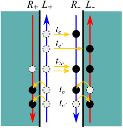
Finally, we include the two-particle backscattering across the junction,

$$H_{\text{junc}}^{(I)}= -t_{\sigma}\left[L^{\dagger}_{+}(0)R_{+}(0)L^{\dagger}_{-}(0)R_{-}(0)+\text{H.c.}\right]$$

$$-t_{\sigma^{\prime}}\left[L^{\dagger}_{+}(0)R_{+}(0)R^{\dagger}_{-}(0)L_{-}(0)+\text{H.c.}\right].$$ (12)

The $t_{\sigma}$ and $t_{\sigma^{\prime}}$ processes can be viewed as “spin-flip” processes. In particular, $t_{\sigma^{\prime}}$ operator breaks the nongeneric spin $S_{z}$ conservation Teo and Kane (2009). These two interactions are analogous to the primary inter-edge interactions in the studies of helical liquid drag Chou et al. (2015); Chou (2019). When $t_{\sigma}$ and $t_{\sigma^{\prime}}$ are both relevant, the junction becomes a barrier that suppresses electrical conduction and breaks time-reversal symmetry Teo and Kane (2009).

In the presence of time-reversal symmetry one can also consider an interaction-assisted backscattering Chou et al. (2015)

$$H_{\text{junc}}^{(\text{irr})}= -W^{\prime}_{+}\Big{[}R^{\dagger}_{-}(0)L_{-}(0)R^{\dagger}_{+}(0)R_{+}(0)$$

$$\hskip 22.76219pt-L^{\dagger}_{-}(0)R_{-}(0)L^{\dagger}_{+}(0)L_{+}(0)+\text{H.c.}\Big{]}$$

$$-W^{\prime}_{-}\Big{[}R^{\dagger}_{+}(0)L_{+}(0)R^{\dagger}_{-}(0)R_{-}(0)$$

$$\hskip 22.76219pt-L^{\dagger}_{+}(0)R_{+}(0)L^{\dagger}_{-}(0)L_{+}(0)-\text{H.c.}\Big{]}.$$ (13)

However, standard RG analysis shows that it and all other perturbations are irrelevant. Thus, in the remaining discussion we will focus on $H_{\text{hLL},2}+H_{\text{junc}}^{(1)}+H_{\text{junc}}^{(2)}+H_{\text{juct}}^{(I)}$, processes, summarized in Fig. 3.

To study the above processes in the presence of Luttinger liquid interactions, we employ standard bosonization Shankar (2017); Giamarchi (2004) of the above Hamiltonian. With the detailed derivation relegated to Appendix B, below we summarize the results of the leading order renormalization group analysis, with the RG flow equations given by

$$\frac{dt_{e}}{dl}= \left[1-\frac{1}{2}\left(K+\frac{1}{K}\right)\right]t_{e},$$ (14a)

$$\frac{dt_{e^{\prime}}}{dl}= \left[1-\frac{1}{2}\left(K+\frac{1}{K}\right)\right]t_{e^{\prime}},$$ (14b)

$$\frac{dt_{2e}}{dl}= \left[1-\frac{2}{K}\right]t_{2e},$$ (14c)

$$\frac{dt_{\sigma}}{dl}= \left[1-2K\right]t_{\sigma},$$ (14d)

$$\frac{dt_{\sigma^{\prime}}}{dl}= \left[1-2K\right]t_{\sigma^{\prime}}.$$ (14e)

These are consistent with the previous works on the corner junction Hou et al. (2009) and the quantum point contact Teo and Kane (2009). We also note that $t_{e}$ and $t_{e^{\prime}}$ are at most marginal in the noninteracting limit, $K=1$. This ensures that the configuration of two helical states we consider is unchanged in the repulsive interaction regime. The Cooper pair tunneling $t_{2e}$ naturally becomes relevant for sufficiently strong attractive interactions ($K>2$). Thus, below we focus on the two-particle backscattering, $t_{\sigma}$ and $t_{\sigma^{\prime}}$, that become relevant for $K<1/2$.

For such strongly repulsive interactions, $K<1/2$, we only need to consider $H_{\text{hLL},2}+H_{\text{junc}}^{(I)}$. As detailed in Appendix B, the inter-domain-wall coupling decomposes the action into symmetric and antisymmetric sectors. In each sector, the action can be mapped to the Kane-Fisher model Kane and Fisher (1992a, b) with $K\rightarrow 2K$. For $K<1/2$, the impurity interactions effectively cut (i.e., pin) the symmetric and antisymmetric Luttinger liquids. In the physical basis of two helical Luttinger liquids, the junction coupling creates a perfectly reflecting boundary condition which suppresses all conduction Teo and Kane (2009). The junction is therefore “clogged.” Concomitantly, the time-reversal symmetry is broken spontaneously and heterogeneously by the network of junctions Teo and Kane (2009).

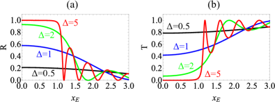
At the critical point $K=1/2$, the transmission across a single junction is nonzero and can be computed exactly by fermionizing the symmetric and antisymmetric sectors into a noninteracting model of Luther-Emery fermions. The scattering problem can then be solved exactly, with the physical transmission (T) and reflection (R) coefficients given by Teo and Kane (2009),

$$\text{T}=\left(\frac{2e^{|M_{b}|/v}}{e^{2|M_{b}|/v}+1}\right)^{2},$$ (15a)

$$\text{R}=\left(\frac{e^{2|M_{b}|/v}-1}{e^{2|M_{b}|/v}+1}\right)^{2},$$ (15b)

where $b=S,A$ indicates symmetric and antisymmetric sectors. Above, $M_{S}=t_{\sigma}/(\pi\alpha)$ and $M_{A}=t_{\sigma^{\prime}}/(\pi\alpha)$, with $\alpha$ the ultraviolet length-scale cutoff. We note that the expressions are independent of the energy due to low-energy point-scattering approximation. When $|M_{b}|/v\gg 1$, the transmission $\text{T}\approx 4\exp(-2|M_{b}|/v)$. Therefore, we conclude that the junction at $K=1/2$ is also clogged for $|M_{b}|/v\gg 1$. The details of this analysis, extended beyond a point junction limit is relegated to Appendix B.

The above results can now be bootstrapped to characterize the helical network surface of clogged junctions. The surface can be viewed as a network of ideal helical conductors that are connected by clogged resistive junctions. Each clogged junction contributes incoherently a suppression factor $G_{j}\sim\exp\left(-2|M_{j}|/v\right)$, where $j$ is the junction index and $|M_{j}|$ is the amplitude of the effective potential. The conductance is determined by the most conductive path in the network. We estimate the conductance by $G\sim\prod_{j}^{\prime}G_{j}\sim\exp\left(-2\sum_{j}^{\prime}|M_{j}|/v\right)$, where the summation runs over all the junctions in the most conductive path. Without loss of generality, the number of the junctions in the path is roughly $L/l_{\text{seg}}$ ($l_{\text{seg}}$ the typical length of the domain-wall segment). Combining the above estimates, we predict a surface conductance $G\sim\exp(-2\frac{\bar{M}}{v}\frac{L}{l_{\text{seg}}})$ where $\bar{M}$ is the averaged value of $|M_{j}|$. As a comparison, the conductance in the localized regime is $G\sim\exp\left(-2L/\xi_{\text{loc}}\right)$, where $\xi_{\text{loc}}$ is the averaged localization length. The exponentially small conductance of the clogged state and the absence of qualitative distinctions, argues that these regimes are a single localized state, separated by a smooth crossover, rather than a genuine phase transition.

V Discussion and summary

We explored the stability of a 2D metallic surface of a 3D spin chiral (CII class) topological insulator to disorder and interaction. In the scenario of a symmetry broken surface that forms multiple statistically symmetric domains, we argued that the surface can realize a gapless insulating ground state, with two regimes - a network of 1D helical domain-walls interrupted by blockaded junctions (the clogged regime), and a network of localized 1D helical channels (the fully-localized regime). This gapless insulating surface state, realized only in the CII TI class, is a distinct scenario from the previously discussed possibilities of interacting TI surfaces Vishwanath and Senthil (2013); Wang and Senthil (2013, 2014); Metlitski et al. (2014); Senthil (2015).

The gapless insulating surface of nontrivial TIs predicted here shares many experimental features with a 2D conventional Anderson insulator, exhibiting vanishing dc conductivity and nonzero compressibility. However, it may be distinguishable through real-space surface imaging (e.g., STM) by its low-energy states organized into the characteristic domain-wall network, quite different from the conventional 2D localized states. In addition, the half-charge excitations in the localized regime Chou et al. (2018) and the perfect barrier junctions Teo and Kane (2009) should in principle be experimentally detectable via noise measurements.

Finite temperature and finite frequency measurements may also be able to distinguish between the clogged and fully-localized regimes, tunable by the strength of interactions and disorder, with the latter controlling the domain size. In the clogged regime of the dilute domain-wall limit the temperature dependence of the surface transport is dictated by the weak junction links Kane and Fisher (1992b, a) and should then exhibit the one-dimensional insulator dependence. The ac conductivity will show a crossover frequency scale set by $\omega^{*}\sim v_{F}/l_{\text{seg}}$ ($l_{\text{seg}}$ the length of domain-wall segment) above which the ac conductivity is the same as that of a 1D helical liquid Kainaris et al. (2014). In contrast, at low frequency ($\omega<\omega^{*}$) the ac conductivity should vanish due to the weak link barriers at the junctions.

In the fully-localized regime, the transport is governed by a network of one-dimensional localized insulators. The low temperature conductance due to a localized insulator should follow $G\sim e^{-2L/\xi_{\text{loc}}}$, where $\xi_{\text{loc}}$ is the localization length. The ac conductivity should show the Mott conductivity $\sigma\propto\omega^{2}$ Mott (1968) up to logarithmic corrections. These two regimes are connected via a crossover for finite domain-wall segments and become distinct phases in the infinite domain-wall segment limit.

In this work, we consider statistically symmetry-preserving disorder that creates inhomogeneous symmetry breaking. Such disorder may be generated due to the interplay of symmetric disorder and interaction, leading to instabilities of the dirty interacting topological surface states Foster and Yuzbashyan (2012); Nandkishore et al. (2013); Foster et al. (2014). A systematic derivation of the heterogeneous spontaneous symmetry breaking in a dirty interacting TI is beyond the scope of the current work and is left to future studies.

We note that the clogged state predicted here may also be realized in the Luttinger liquid networks of the (twisted) bilayer graphene and other related platforms Zhang et al. (2013); San-Jose and Prada (2013); Hattendorf et al. (2013); Alden et al. (2013); Ju et al. (2015); Yin et al. (2016); Li et al. (2016, 2017b); Tong et al. (2017); Efimkin and MacDonald (2018); Huang et al. (2018); Wu et al. (2018). If so, the clogged phenomenology predicted here may extend to those systems as well. We leave to future work the extension of the present analysis to six-way junctions, relevant in the twisted bilayer graphene systems Hattendorf et al. (2013); Alden et al. (2013).

Appendix A Derivations of domain-wall states

Here we derive the low-energy domain-wall model from the 2D surface theory encoded in $H_{0}+H_{\text{dis}}+H_{\text{M},a}$, Eqs. (1), (2), and (4). Our strategy is to first solve $H_{0}+H_{\text{M},a}$ exactly, thereby obtaining the domain-wall states and then treat $H_{\text{dis}}$ as a perturbation. The solution of $H_{0}+H_{\text{M},a}$ can be parametrized by $\Psi_{0}(x,y)=f(x)\left[\tilde{\psi}_{1}(y)\hat{v}_{1}+\tilde{\psi}_{2}(y)\hat{v}_{2}\right]$ where $\tilde{\psi}_{1,2}(y)$ are normalized wavefunctions of $y$ and $\hat{v}_{1,2}$ is a four component vector. Taking $m_{a}(x)=m_{a}\operatorname{sgn}(x)$, we find that the amplitude $f(x)$ and vectors $\hat{v}_{1,2}$ satisfy,

$$-iv_{D}\hat{\sigma}^{x}\hat{v}_{1,2}\partial_{x}f(x)+m_{a}\operatorname{sgn}(x)\hat{M}_{a}\hat{v}_{1,2}f(x)=0,$$ (16)

which reduces to

$$\hat{v}_{1,2}\partial_{x}f(x)=-\frac{m_{a}}{v_{D}}\left(i\hat{\sigma^{x}}\hat{M}_{a}\right)\operatorname{sgn}(x)\hat{v}_{1,2}f(x).$$ (17)

The zero energy normalizable amplitude solution is given by

$$f(x)=\sqrt{\frac{m_{a}}{v_{D}}}e^{-(m_{a}/v_{D})|x|},$$ (18)

and the four component vectors satisfy

$$i\hat{\sigma}^{x}\hat{M}_{a}\hat{v}_{1,2}=\hat{v}_{1,2}.$$ (19)

The above solution $f(x)$ describes the domain-wall profile across $x$, with the domain-wall chosen to run along $y$. The single domain-wall assumption is justified as long as its width $(v_{D}/m_{a})$ is much smaller than the typical domain size $w$, i.e., $wm_{a}/v_{D}\gg 1$.

To obtain the effective 1D domain-wall Hamiltonian we substitute $\Psi_{0}$ for $\Psi$ inside $H_{0}+H_{\text{dis}}+H_{\text{M},a}$. The resulting kinetic energy part of the domain-wall Hamiltonian is then given by

$$H_{\text{DW},0}= \left[H_{0}+H_{\text{M},a}\right]_{\Psi\rightarrow\Psi_{0}}$$

$$= v_{D}\int dy\left[-is_{1}\tilde{\psi}_{1}^{\dagger}\partial_{y}\tilde{\psi}_{1}-is_{2}\tilde{\psi}_{2}^{\dagger}\partial_{y}\tilde{\psi}_{2}\right],$$ (20)

where $s_{1,2}=\hat{v}_{1,2}^{\dagger}\hat{\sigma}^{y}\hat{v}_{1,2}=\pm 1$ determines the sign of velocities for the fermion fields $\psi_{i}$. The domain-wall model is chiral when $s_{1}=s_{2}$. We note that there is no mixing term because $[\hat{\sigma}^{x}\hat{M}_{a},\hat{\sigma}^{y}]=0$.

The disorder part of the Hamiltonian is given by

$$H_{\text{DW,dis}}=H_{\text{dis}}\left[\Psi\rightarrow\Psi_{0}\right],$$

$$= \sum_{a,b}\int dy\,\tilde{\psi}_{a}^{\dagger}\hat{v}_{a}^{\dagger}\left[\tilde{v}_{1}\hat{\tau}^{x}+\tilde{v}_{2}\hat{\tau}^{z}+\tilde{a}_{1}\hat{\sigma}^{x}\hat{\tau}^{y}+\tilde{a}_{2}\hat{\sigma}^{y}\hat{\tau}^{y}\right]\hat{v}_{b}\tilde{\psi}_{b},$$ (21)

where $a,b=1,2$ are the one-dimensional fermion flavors. The 1D disorder bilinears, $\tilde{v}_{1}$, $\tilde{v}_{2}$, $\tilde{a}_{1}$, and $\tilde{a}_{2}$, correspond to their 2D disorder counter-parts, $v_{1}$, $v_{2}$, $a_{1}$, and $a_{2}$, respectively, related by, $\tilde{\mathcal{O}}(y)=\int dxf^{2}(x)\mathcal{O}(x,y)$ for $\mathcal{O}=v_{1},v_{2},a_{1},a_{2}$.

We now use this set up to derive and analyze the structure of the chiral, helical, and (fine-tuned) non-topological domain-walls.

A.1 Chiral domain-walls

In the presence of only $\hat{M}_{1}=\hat{\sigma}^{z}$ mass operator, the time-reversal symmetry ($\mathcal{T}$) is broken, but the particle-hole ($\mathcal{P}$) is preserved. The resulting symmetry-broken surface corresponds to the symmetry class C Altland and Zirnbauer (1997). The corresponding spinor equation reduces to $i\hat{\sigma}^{x}\hat{M}_{1}\hat{v}_{1,2}=\hat{\sigma}^{y}\hat{v}_{1,2}=\hat{v}_{1,2}$, with solutions

$$\hat{v}_{1}=\frac{1}{\sqrt{2}}\left[\begin{array}[]{c}1\\ 0\\ i\\ 0\end{array}\right],\,\,\,\hat{v}_{2}=\frac{1}{\sqrt{2}}\left[\begin{array}[]{c}0\\ 1\\ 0\\ i\end{array}\right].$$ (30)

We can then identify that $s_{1}=\hat{v}_{1}^{\dagger}\hat{\sigma}^{y}\hat{v}_{1}=1$ and $s_{2}=\hat{v}_{2}^{\dagger}\hat{\sigma}^{y}\hat{v}_{2}=1$. Based on the structure in Eq. (20), the domain-wall state only contains right-mover fermions. Thus such a domain-wall solution realizes a chiral state, which corresponds to the spin quantum Hall edge of class C Gruzberg et al. (1997); Senthil et al. (1998); Gruzberg et al. (1999); Senthil et al. (1999), and is robust against any local perturbation within a domain-wall.

For completeness, we also construct the disorder potential on the domain-wall even though a chiral state is robust against such disorder. Using Eqs. (21) and  (30), the effective disorder domain-wall Hamiltonian is given by

$$H_{\text{DW,dis}}^{(1)}\!=\! \int\limits_{y}\!\left[\!\tilde{v}_{2}(y)(\psi^{\dagger}_{1}\psi_{1}-\psi^{\dagger}_{2}\psi_{2})\!+\!\tilde{a}_{2}(y)(i\psi^{\dagger}_{2}\psi_{1}-i\psi^{\dagger}_{1}\psi_{2})\!\right].$$

The above $\tilde{v}_{2}$ plays the role of an anti-symmetric chemical potential in the two right movers, and $\tilde{a}_{y}$ is an impurity forward scattering between two right movers, that cannot induce localization Kane and Fisher (1995).

A.2 Helical domain-walls

We now consider a symmetry-breaking mass $\hat{M}_{2}=\hat{\sigma}^{z}\hat{\tau}^{y}$. This mass bilinear breaks the particle-hole symmetry but preserves time-reversal symmetry. The symmetry-broken surface belongs to the class AII (the same as the 2D time-reversal symmetric $\mathrm{Z}_{2}$ TIs). The corresponding spinor equation is $\hat{\sigma}^{y}\hat{\tau}^{y}\hat{v}_{1,2}=\hat{v}_{1,2}$ and yields solutions

$$\hat{v}_{1}=\frac{1}{2}\left[\begin{array}[]{c}1\\ i\\ i\\ -1\end{array}\right],\,\,\,\hat{v}_{2}=\frac{1}{2}\left[\begin{array}[]{c}1\\ -i\\ -i\\ -1\end{array}\right].$$ (39)

In this case, $s_{1}=\hat{v}_{1}^{\dagger}\hat{\sigma}^{y}\hat{v}_{1}=1$ and $s_{2}=\hat{v}_{2}^{\dagger}\hat{\sigma}^{y}\hat{v}_{2}=-1$. According to Eq. (20), the domain-wall movers are described by a right mover ($s_{1}=1$) and a left mover ($s_{2}=-1$). In order to assess the effect of symmetric disorder, we construct the domain-wall disorder potential Hamiltonian based on Eq. (21), obtaining

$$H_{\text{DW,dis}}^{(2)}=\int\limits_{y}\tilde{a}_{2}(y)\left[\tilde{\psi}^{\dagger}_{1}\tilde{\psi}_{1}+\tilde{\psi}^{\dagger}_{2}\tilde{\psi}_{2}\right].$$ (40)

The domain-wall disorder is controlled by a scalar potential $\tilde{a}_{2}$, corresponding to a randomly fluctuating chemical potential. Based on symmetry, one can also include $\hat{V}_{4}=\hat{1}$ in Table 1. This only creates correction to the existing random chemical potential fluctuation. There are no additional bilinear operators with $\mathcal{T}^{2}=-1$, so we conclude that the domain-wall state is a helical state Potter et al. (2017) which is topologically protected from disorder in the absence of interactions Kane and Mele (2005a).

A.3 Normal domain-wall

For certain microscopic models (e.g., fine tuning interactions such that only $U_{3}\neq 0$ or $U_{4}\neq 0$ appear), it is possible to realize only one mass term. Here, we perform the same analysis to derive the domain-wall states due to only $\hat{M}_{3}=\hat{\sigma}^{z}\hat{\tau}^{x}$ or $\hat{M}_{4}=\hat{\sigma}^{z}\hat{\tau}^{z}$ mass operators. In the two dimensions, the AIII class is topologically trivial. The spinor solutions ($\hat{v}_{1,2}$ for $\hat{M}_{3}$, $\hat{u}_{1,2}$ for $\hat{M}_{4}$) obey $\hat{\sigma}^{y}\hat{\tau}^{x}\hat{v}_{1,2}=\hat{v}_{1,2}$ and $\hat{\sigma}^{y}\hat{\tau}^{z}\hat{u}_{1,2}=\hat{u}_{1,2}$. The corresponding solutions are given by

$$\hat{v}_{1}=\frac{1}{2}\left[\begin{array}[]{c}1\\ 1\\ i\\ i\end{array}\right],\,\,\,\hat{v}_{2}=\frac{1}{2}\left[\begin{array}[]{c}1\\ -1\\ -i\\ i\end{array}\right],$$ (49)

and

$$\hat{u}_{1}=\frac{1}{\sqrt{2}}\left[\begin{array}[]{c}1\\ 0\\ i\\ 0\end{array}\right],\,\,\,\hat{u}_{2}=\frac{1}{\sqrt{2}}\left[\begin{array}[]{c}0\\ 1\\ 0\\ -i\end{array}\right]$$ (58)

We thus identify that $\hat{v}_{1}^{\dagger}\hat{\sigma}^{y}\hat{v}_{1}=\hat{u}_{1}^{\dagger}\hat{\sigma}^{y}\hat{u}_{1}=1$ (right mover) and $\hat{v}_{2}^{\dagger}\hat{\sigma}^{y}\hat{v}_{2}=\hat{u}_{2}^{\dagger}\hat{\sigma}^{y}\hat{u}_{2}=-1$ (left mover). Therefore, both cases give a non-chiral state. Because the surface state is in class A, the massless domain-wall hosts non-topological 1D fermions.

For completeness, we also discuss the corresponding domain-wall disorder. With the mass $\hat{M}_{3}$, the disorder part is given by

$$H_{\text{DW,dis}}^{(3)}= \int\limits_{y}\tilde{v}_{1}(y)\left[\tilde{\psi}^{\dagger}_{1}\tilde{\psi}_{1}-\tilde{\psi}^{\dagger}_{2}\tilde{\psi}_{2}\right]$$

$$+\int\limits_{y}\tilde{a}_{1}(y)\left[\tilde{\psi}^{\dagger}_{2}\tilde{\psi}_{1}+\tilde{\psi}^{\dagger}_{1}\tilde{\psi}_{2}\right].$$ (59)

For $\hat{M}_{4}$ case we instead find,

$$H_{\text{DW,dis}}^{(4)}= \int\limits_{y}\tilde{v}_{2}(y)\left[\tilde{\psi}^{\dagger}_{1}\tilde{\psi}_{1}-\tilde{\psi}^{\dagger}_{2}\tilde{\psi}_{2}\right]$$

$$-\int\limits_{y}\tilde{a}_{1}(y)\left[\tilde{\psi}^{\dagger}_{2}\tilde{\psi}_{1}+\tilde{\psi}^{\dagger}_{1}\tilde{\psi}_{2}\right].$$ (60)

The antisymmetry chemical potentials ($\tilde{v}_{1}$ in $H_{\text{DW,dis}}^{(3)}$ and $\tilde{v}_{2}$ in $H_{\text{DW,dis}}^{(4)}$ ) couples to the difference of right and left mover local densities. Both cases allow for conventional impurity backscattering ($\tilde{a}_{1}$ in both cases) within the domain wall, and thus realizes topologically trivial 1D fermions, which are therefore not protected against Anderson localization.

Appendix B Helical junction

In this appendix, we provide the derivations of the results in Sec. IV.2. We will also review the standard bosonization and the Luther-Emery analysis.

B.1 Bosonization

To treat the Luttinger interaction nonperturbatively, we adopt the standard field theoretic bosonization method Shankar (2017). The fermionic fields can be described by chiral bosons via

$$R_{a}(x)=\frac{\hat{U}_{a}}{\sqrt{2\pi\alpha}}e^{i\left[\phi_{a}+\theta_{a}\right](x)},\,\,L_{a}(x)=\frac{\hat{U}_{a}}{\sqrt{2\pi\alpha}}e^{i\left[\phi_{a}-\theta_{a}\right](x)},$$ (61)

where $\phi_{a=\pm}$ is the bosonic phase field, $\theta_{a=\pm}$ is the phonon-like boson, $U_{a=\pm}$ is the Klein factor Giamarchi (2004), and $\alpha$ is the ultraviolet length scale that is determined by the microscopic model. The time-reversal operation ($\mathcal{T}^{2}=-1$) in the bosonic language is defined as follows: $\phi_{\pm}\rightarrow-\phi_{\pm}+\frac{\pi}{2}$, $\theta_{\pm}\rightarrow\theta_{\pm}-\frac{\pi}{2}$, and $i\rightarrow-i$. This corresponds to the fermionic operation $R_{\pm}\rightarrow L_{\pm}$, $L_{\pm}\rightarrow-R_{\pm}$, and $i\rightarrow-i$. We note that the introduction of the Klein factors ($U_{a=\pm}$) here is just for bookkeeping purposes.

Now, we perform the standard bosonization and analyze the Hamiltonian. The Hamiltonian of each helical liquid is bosonized to

$$H_{\text{hLL},2}=\sum_{a=\pm}\int\limits_{x}\left[\frac{v}{2\pi K}\left(\partial_{x}\theta_{a}\right)^{2}+\frac{vK}{2\pi}\left(\partial_{x}\phi_{a}\right)^{2}\right],$$ (62)

where we have assumed the same velocity ($v$) and the same Luttinger parameter ($K$) among the two helical liquids. $K$ encodes the strength Luttinger liquid interactions. $K<1$ ($K>1$) for repulsive (attractive) interactions. $K=1$ is at the non-interacting fermion limit. The impurity perturbations [given by Eqs. (10), (11), and (12)] are bosonized to

$$H_{\text{junc}}^{(1)}= -\frac{t_{e}}{2\pi\alpha}\left[\hat{U}_{-}^{\dagger}\hat{U}_{+}(2i)e^{i(\phi_{+}-\phi_{-})}\sin\left(\theta_{+}+\theta_{-}\right)+\text{H.c.}\right]$$

$$-\frac{t_{e^{\prime}}}{2\pi\alpha}\left[\hat{U}_{-}^{\dagger}\hat{U}_{+}2e^{i(\phi_{+}-\phi_{-})}\cos\left(\theta_{+}-\theta_{-}\right)+\text{H.c.}\right],$$ (63)

$$H_{\text{junc}}^{(2)}= -\frac{t_{2e}}{4\pi\alpha^{2}}\left[\hat{U}_{-}^{\dagger}\hat{U}_{-}^{\dagger}\hat{U}_{+}\hat{U}_{+}e^{i(2\phi_{+}-2\phi_{-})}+\text{H.c.}\right],$$ (64)

$$H_{\text{junc}}^{(I)}= -\frac{t_{\sigma}}{2\pi^{2}\alpha^{2}}\cos\left[2\theta_{+}+2\theta_{-}\right]-\frac{t_{\sigma^{\prime}}}{2\pi^{2}\alpha^{2}}\cos\left[2\theta_{+}-2\theta_{-}\right].$$ (65)

The corresponding renormalization group equations can be found in Eq. (14).

B.2 Clogged junction

We are interested in the repulsive interacting regime ($K<1$) in the helical network model. Therefore, we focus on the $t_{\sigma}$ and $t_{\sigma^{\prime}}$ interactions given by Eq. (65) and ignore other processes. In the strong coupling limit ($K<1/2$), the ground state constraints are $\theta_{+}(t,x=0)+\theta_{-}(t,x=0)=n\pi$ and $\theta_{+}(t,x=0)+\theta_{-}(t,x=0)=m\pi$ where $n$ and $m$ are integers. The ground state yields static solutions at $x=0$: $\theta_{+}(t,x=0)=(n+m)\pi/2$ and $\theta_{-}(t,x=0)=(n-m)\pi/2$. As a consequence, the current $I_{\pm}=-\frac{1}{\pi}\partial_{t}\theta_{\pm}$ at $x=0$ is zero in both of the helical liquids. Therefore, we predict that a four-way junction with semi-infinite helical liquids becomes “clogged” for $K<1/2$.

An alternative way to view the clogging is to map the problem to a modified Kane-Fisher single impurity problem Kane and Fisher (1992b, a). We define symmetric and anti-symmetric collective bosonic modes as follows:

$$\Theta_{S}= \frac{1}{\sqrt{2}}(\theta_{+}+\theta_{-}),\,\,\Phi_{S}=\frac{1}{\sqrt{2}}(\phi_{+}+\phi_{-}),$$ (66)

$$\Theta_{A}= \frac{1}{\sqrt{2}}(\theta_{+}-\theta_{-}),\,\,\Phi_{A}=\frac{1}{\sqrt{2}}(\phi_{+}-\phi_{-}).$$ (67)

The subscript $S$ and $A$ denote the symmetric and anti-symmetric collective modes respectively. Now, we use the collective coordinate to rewrite the theory. The Luttinger liquid Hamiltonian in Eq. (62) is now expressed by

$$H_{\text{hLL},2}= \int\limits_{x}\left[\frac{v}{2\pi K}\left(\partial_{x}\Theta_{S}\right)^{2}+\frac{vK}{2\pi}\left(\partial_{x}\Phi_{S}\right)^{2}\right]$$ (68)

$$+\int\limits_{x}\left[\frac{v}{2\pi K}\left(\partial_{x}\Theta_{A}\right)^{2}+\frac{vK}{2\pi}\left(\partial_{x}\Phi_{A}\right)^{2}\right].$$ (69)

We note that the impurity interaction can not induce renormalization of the velocity and Luttinger parameter. The junction interactions in Eq. (65) becomes to

$$H_{\text{junc}}^{(I)}=-\frac{t_{\sigma}}{2\pi^{2}\alpha^{2}}\cos\left[2\sqrt{2}\Theta_{S}\right]-\frac{t_{\sigma^{\prime}}}{2\pi^{2}\alpha^{2}}\cos\left[2\sqrt{2}\Theta_{A}\right].$$ (70)

Both the symmetric and anti-symmetric sectors can be individually mapped to the Kane-Fisher problem Kane and Fisher (1992a, b) with $K\rightarrow 2K$. The critical point is given by $K=1/2$ below which the transmission of both the symmetric and anti-symmetric modes vanish to zero.

B.3 Luther-Emery Analysis

At the critical point $K=1/2$, one can perform standard refermionization for the two helical Luttinger liquids problem since both the symmetric and the anti-symmetric sectors correspond to the Kane-Fisher model Kane and Fisher (1992b, a). We introduce the Luther-Emery fermions via

$$\Psi_{b,R}(x)= \frac{e^{i\left[\Phi_{b}(x)/\sqrt{2}+\sqrt{2}\Theta_{b}(x)\right]}}{\sqrt{2\pi\alpha}},$$

$$\Psi_{b,L}(x)= \frac{e^{i\left[\Phi_{b}(x)/\sqrt{2}-\sqrt{2}\Theta_{b}(x)\right]}}{\sqrt{2\pi\alpha}},$$ (71)

where $b=S,A$ is the index for symmetric ($S$) and antisymmetric ($A$) collective modes. The Luther-Emery fermion Hamiltonian of the sector $b$ is given by

$$H_{b}= -iv\int dx\left[\Psi^{\dagger}_{b,R}\partial_{x}\Psi_{b,R}-\Psi^{\dagger}_{b,L}\partial_{x}\Psi_{b,L}\right]$$

$$+M_{b}\left[\Psi^{\dagger}_{b,R}\Psi_{b,L}+\Psi^{\dagger}_{b,L}\Psi_{b,R}\right]_{x=0},$$ (72)

where $M_{b=S}=t_{\sigma}/(\pi\alpha)$ and $M_{b=A}=t_{\sigma^{\prime}}/(\pi\alpha)$. The impurity mass problem can be solved via standard quantum mechanical scattering approach. First, we derive the Dirac equation as follows:

$$\left[\begin{array}[]{cc}-iv\partial_{x}&M_{b}\delta(x)\\ M_{b}\delta(x)&iv\partial_{x}\end{array}\right]\left[\begin{array}[]{c}\Psi_{b,R}\\ \Psi_{b,L}\end{array}\right]=E\left[\begin{array}[]{c}\Psi_{b,R}\\ \Psi_{b,L}\end{array}\right]$$ (79)

$$\rightarrow -iv\hat{\sigma}^{z}\partial_{x}\hat{\Psi}_{b}+M_{b}\delta(x)\hat{\sigma}^{x}\hat{\Psi}_{b}=E\hat{\Psi}_{b},$$ (80)

where $\hat{\Psi}_{b}$ is the two-component column vector that contains $\Psi_{b,R}$ and $\Psi_{b,L}$. The above equation satisfies a boundary condition as follows:

$$-iv\hat{\sigma}^{z}\left[\hat{\Psi}_{b}(0^{+})-\hat{\Psi}_{b}(0^{-})\right]+M_{b}\hat{\sigma}^{x}\hat{\Psi}_{b}(0)=0.$$ (81)

We note that this boundary condition is ambiguous because the wavefunction might be discontinuous at $x=0$.

Figure 4: Reflection and transmission of 1D Dirac scattering problem (finite mass region) as functions of rescaled energy. (a) Reflection, $\text{R}=|A|^{2}$. (b) Transmission, $\text{T}=|D|^{2}$. Both $A$ and $B$ are given by Eq. (87). $x_{E}$ is the dimensionless energy parameter defined in the text below Eq. (87). Black, blue, green, and red curves indicate $\Delta=M_{b}/v=0.5,1,2,5$ respectively. The perfect transmissions (T$=1$ and R$=0$) for $x_{E}>1$ correspond to the Fabry-Pérot interference.

Instead of studying the delta distribution problem, we replace the impurity potential by a square well potential, $M_{b}\delta(x)\rightarrow\tilde{M}_{b}\Theta(x)\Theta(d-x)$, where $d$ is the size of mass region and $\tilde{M}_{b}=M_{b}/d$ is the “mass” strength. The impurity limit is obtained by taking $d\rightarrow 0^{+}$. With a finite $d$, the wavefunction is continuous everywhere because of the analyticity. We consider a scattering ansatz as follows:

$$\hat{\Psi}_{b}(x)\!=\!\begin{cases}e^{ikx}\left[\begin{array}[]{c}1\\ 0\end{array}\right]+Ae^{-ikx}\left[\begin{array}[]{c}0\\ 1\end{array}\right],&\text{for }x\leq 0,\\[11.38109pt] Be^{iqx}\!\!\left[\!\!\begin{array}[]{c}1\\ \frac{-vq+E}{\tilde{M}_{b}}\end{array}\!\!\right]\!+\!Ce^{-iqx}\!\!\left[\!\!\begin{array}[]{c}\frac{-vq+E}{\tilde{M}_{b}}\\ 1\end{array}\!\!\right],&\text{for }0\!<\!x\!\leq\!d,\\[11.38109pt] De^{ikx}\left[\begin{array}[]{c}1\\ 0\end{array}\right],&\text{for }x>d,\end{cases}$$ (82)

where $k=E/v$ and $q=\sqrt{E^{2}-\tilde{M}_{b}^{2}}/v$. The boundary conditions are given by

$$B+C\left(\frac{-vq+E}{\tilde{M}_{b}}\right)= 1,$$ (83)

$$B\left(\frac{-vq+E}{\tilde{M}_{b}}\right)+C= A,$$ (84)

$$Be^{iqd}+Ce^{-iqd}\left(\frac{-vq+E}{\tilde{M}_{b}}\right)= De^{ikd},$$ (85)

$$Be^{iqd}\left(\frac{-vq+E}{\tilde{M}_{b}}\right)+Ce^{-iqd}= 0.$$ (86)

With the help of Mathematica, one can obtain the solutions as follows:

$$A= \frac{\left(\sqrt{x_{E}^{2}-1}-x_{E}\right)\left(-1+e^{2i\Delta\sqrt{x_{E}^{2}-1}}\right)}{1+\left(2x_{E}\sqrt{x_{E}^{2}-1}-2x_{E}^{2}+1\right)e^{2i\Delta\sqrt{x_{E}^{2}-1}}},$$ (87a)

$$B= \frac{1}{1+\left(2x_{E}\sqrt{x_{E}^{2}-1}-2x_{E}^{2}+1\right)e^{2i\Delta\sqrt{x_{E}^{2}-1}}},$$ (87b)

$$C= \frac{\left(\sqrt{x_{E}^{2}-1}-x_{E}\right)e^{2i\Delta\sqrt{x_{E}^{2}-1}}}{1+\left(2x_{E}\sqrt{x_{E}^{2}-1}-2x_{E}^{2}+1\right)e^{2i\Delta\sqrt{x_{E}^{2}-1}}},$$ (87c)

$$D= \frac{2\left(x_{E}\sqrt{x_{E}^{2}-1}-x_{E}^{2}+1\right)e^{i\Delta\left(\sqrt{x_{E}^{2}-1}-x_{E}\right)}}{1+\left(2x_{E}\sqrt{x_{E}^{2}-1}-2x_{E}^{2}+1\right)e^{2i\Delta\sqrt{x_{E}^{2}-1}}},$$ (87d)

where $x_{E}\equiv E/|\tilde{M}_{b}|$ and $\Delta\equiv d|\tilde{M}_{b}|/v=|M_{b}|/v$. The reflection is $\text{R}=|A|^{2}$ and transmission is $\text{T}=|D|^{2}$. The dependence of $x_{E}$ and $\Delta$ are plotted in Fig. 4. For $\Delta=|M_{b}|/v\gg 1$, the scattering problem reveals a sharp gap structure because $\text{R}\approx 1$ for $x_{E}<1$. For $x_{E}>1$, there are some special energies that allow perfect transmission. This is related to the Fabry-Pérot interference. However, we do not focus on such high energy phenomenon in this work.

Now, we consider $d\rightarrow 0^{+}$ with $\tilde{M}_{b}d=M_{b}$ fixed. The finite mass region is reduced to a single impurity potential. In the impurity case, $x_{E}=Ed/|M_{b}|\rightarrow 0$ for a fixed $M_{b}/v$. The expression of transmission and reflection are reduced to Eq. (15). The results do not depend on the energy due to the infinite $|\tilde{M}_{b}|=|M_{b}|/d$ in this limit. These results characterize the low energy scattering in the network model. In particular, the transmission $\text{T}\rightarrow 4e^{-2|M_{b}|/v}$ when $|M_{b}|/v\gg 1$.

In the four-way junction problem, the clogging conditions at $K=1/2$ correspond to perfect reflections in both the symmetric and antisymmetric sectors. In the zero energy limit, the clogging conditions are $|M_{S}|/v\gg 1$ and $|M_{A}|/v\gg 1$. To make the junction more realistic, we can assume that both the domain-wall segment and the interacting region are finite. The longest wavelength is set by the typical domain-wall segment length, $l_{\text{seg}}$, corresponding to the lowest kinetic energy $E_{0}=v({2\pi}/{l_{\text{seg}}})$. The clogging conditions become to $v({2\pi}/{l_{\text{seg}}})<|t_{\sigma}|/(\pi\alpha d)$, $v({2\pi}/{l_{\text{seg}}})<|t_{\sigma^{\prime}}|/(\pi\alpha d)$, $|t_{\sigma}|/(v\pi\alpha)\gg 1$, and $|t_{\sigma^{\prime}}|/(v\pi\alpha)\gg 1$. The former two conditions are from comparing the energy of the electron to the local mass; the latter two conditions are related to the existence of sharp gaps.

References

- Hasan and Kane (2010) M. Z. Hasan and C. L. Kane, Rev. Mod. Phys. 82, 3045 (2010).
- Qi and Zhang (2011) X.-L. Qi and S.-C. Zhang, Rev. Mod. Phys. 83, 1057 (2011).
- Chiu et al. (2016) C.-K. Chiu, J. C. Y. Teo, A. P. Schnyder, and S. Ryu, Rev. Mod. Phys. 88, 035005 (2016).
- Ludwig (2015) A. W. Ludwig, Physica Scripta 2016, 014001 (2015).
- Anderson (1958) P. W. Anderson, Phys. Rev. 109, 1492 (1958).
- Evers and Mirlin (2008) F. Evers and A. D. Mirlin, Rev. Mod. Phys. 80, 1355 (2008).
- Ando and Fu (2015) Y. Ando and L. Fu, Annu. Rev. Condens. Matter Phys. 6, 361 (2015).
- Mizushima et al. (2016) T. Mizushima, Y. Tsutsumi, T. Kawakami, M. Sato, M. Ichioka, and K. Machida, Journal of the Physical Society of Japan 85, 022001 (2016), https://doi.org/10.7566/JPSJ.85.022001 .
- Vishwanath and Senthil (2013) A. Vishwanath and T. Senthil, Phys. Rev. X 3, 011016 (2013).
- Wang and Senthil (2013) C. Wang and T. Senthil, Phys. Rev. B 87, 235122 (2013).
- Wang and Senthil (2014) C. Wang and T. Senthil, Phys. Rev. B 89, 195124 (2014).
- Metlitski et al. (2014) M. A. Metlitski, L. Fidkowski, X. Chen, and A. Vishwanath, arXiv preprint arXiv:1406.3032 (2014).
- Senthil (2015) T. Senthil, Annual Review of Condensed Matter Physics 6, 299 (2015), https://doi.org/10.1146/annurev-conmatphys-031214-014740 .
- Xu and Moore (2006) C. Xu and J. E. Moore, Phys. Rev. B 73, 045322 (2006).
- Wu et al. (2006) C. Wu, B. A. Bernevig, and S.-C. Zhang, Phys. Rev. Lett. 96, 106401 (2006).
- Chou et al. (2018) Y.-Z. Chou, R. M. Nandkishore, and L. Radzihovsky, Phys. Rev. B 98, 054205 (2018).
- Kane and Mele (2005a) C. L. Kane and E. J. Mele, Phy. Rev. Lett. 95, 146802 (2005a).
- Kane and Mele (2005b) C. L. Kane and E. J. Mele, Phy. Rev. Lett. 95, 226801 (2005b).
- Bernevig and Zhang (2006) B. A. Bernevig and S.-C. Zhang, Phys. Rev. Lett. 96, 106802 (2006).
- Luther and Emery (1974) A. Luther and V. J. Emery, Phys. Rev. Lett. 33, 589 (1974).
- Du et al. (2015) L. Du, I. Knez, G. Sullivan, and R.-R. Du, Phys. Rev. Lett. 114, 096802 (2015).
- Li et al. (2015) T. Li, P. Wang, H. Fu, L. Du, K. A. Schreiber, X. Mu, X. Liu, G. Sullivan, G. A. Csáthy, X. Lin, and R.-R. Du, Phys. Rev. Lett. 115, 136804 (2015).
- Du et al. (2017) L. Du, T. Li, W. Lou, X. Wu, X. Liu, Z. Han, C. Zhang, G. Sullivan, A. Ikhlassi, K. Chang, and R.-R. Du, Phys. Rev. Lett. 119, 056803 (2017).
- Li et al. (2017a) T. Li, P. Wang, G. Sullivan, X. Lin, and R.-R. Du, Phys. Rev. B 96, 241406 (2017a).
- Morimoto et al. (2015a) T. Morimoto, A. Furusaki, and C. Mudry, Phys. Rev. B 91, 235111 (2015a).
- Morimoto et al. (2015b) T. Morimoto, A. Furusaki, and C. Mudry, Phys. Rev. B 92, 125104 (2015b).
- Song and Schnyder (2017) X.-Y. Song and A. P. Schnyder, Phys. Rev. B 95, 195108 (2017).
- Potter et al. (2017) A. C. Potter, C. Wang, M. A. Metlitski, and A. Vishwanath, Phys. Rev. B 96, 235114 (2017).
- Teo and Kane (2009) J. C. Y. Teo and C. L. Kane, Phys. Rev. B 79, 235321 (2009).
- Schnyder et al. (2008) A. P. Schnyder, S. Ryu, A. Furusaki, and A. W. W. Ludwig, Phys. Rev. B 78, 195125 (2008).
- Hosur et al. (2010) P. Hosur, S. Ryu, and A. Vishwanath, Phys. Rev. B 81, 045120 (2010).
- Ryu et al. (2012) S. Ryu, C. Mudry, A. W. W. Ludwig, and A. Furusaki, Phys. Rev. B 85, 235115 (2012).
- Ludwig et al. (1994) A. W. W. Ludwig, M. P. A. Fisher, R. Shankar, and G. Grinstein, Phys. Rev. B 50, 7526 (1994).
- Fulga et al. (2014) I. C. Fulga, B. van Heck, J. M. Edge, and A. R. Akhmerov, Phys. Rev. B 89, 155424 (2014).
- Jackiw and Rebbi (1976) R. Jackiw and C. Rebbi, Phys. Rev. D 13, 3398 (1976).
- Su et al. (1979) W. P. Su, J. R. Schrieffer, and A. J. Heeger, Phys. Rev. Lett. 42, 1698 (1979).
- Gruzberg et al. (1997) I. A. Gruzberg, N. Read, and S. Sachdev, Phys. Rev. B 55, 10593 (1997).
- Senthil et al. (1998) T. Senthil, M. P. A. Fisher, L. Balents, and C. Nayak, Phys. Rev. Lett. 81, 4704 (1998).
- Gruzberg et al. (1999) I. A. Gruzberg, A. W. W. Ludwig, and N. Read, Phys. Rev. Lett. 82, 4524 (1999).
- Senthil et al. (1999) T. Senthil, J. B. Marston, and M. P. A. Fisher, Phys. Rev. B 60, 4245 (1999).
- Xie et al. (2016) H.-Y. Xie, H. Li, Y.-Z. Chou, and M. S. Foster, Phys. Rev. Lett. 116, 086603 (2016).
- Obuse et al. (2007) H. Obuse, A. Furusaki, S. Ryu, and C. Mudry, Phys. Rev. B 76, 075301 (2007).
- Obuse et al. (2008) H. Obuse, A. Furusaki, S. Ryu, and C. Mudry, Phys. Rev. B 78, 115301 (2008).
- Ryu et al. (2010) S. Ryu, C. Mudry, H. Obuse, and A. Furusaki, New Journal of Physics 12, 065005 (2010).
- Obuse et al. (2014) H. Obuse, S. Ryu, A. Furusaki, and C. Mudry, Phys. Rev. B 89, 155315 (2014).
- Hou et al. (2009) C.-Y. Hou, E.-A. Kim, and C. Chamon, Phys. Rev. Lett. 102, 076602 (2009).
- Giamarchi (2004) T. Giamarchi, Quantum physics in one dimension (Oxford Science Publications, 2004).
- Shankar (2017) R. Shankar, Quantum Field Theory and Condensed Matter: An Introduction (Cambridge University Press, 2017).
- Pokrovsky and Talapov (1979) V. L. Pokrovsky and A. L. Talapov, Phys. Rev. Lett. 42, 65 (1979).
- Bocquet (1999) M. Bocquet, Nuclear Physics B 546, 621 (1999).
- Tanaka and Nagaosa (2009) Y. Tanaka and N. Nagaosa, Phys. Rev. Lett. 103, 166403 (2009).
- Chou et al. (2015) Y.-Z. Chou, A. Levchenko, and M. S. Foster, Phys. Rev. Lett. 115, 186404 (2015).
- Chou (2019) Y.-Z. Chou, Phys. Rev. B 99, 045125 (2019).
- Kane and Fisher (1992a) C. L. Kane and M. P. A. Fisher, Phys. Rev. B 46, 15233 (1992a).
- Kane and Fisher (1992b) C. L. Kane and M. P. A. Fisher, Phys. Rev. Lett. 68, 1220 (1992b).
- Kainaris et al. (2014) N. Kainaris, I. V. Gornyi, S. T. Carr, and A. D. Mirlin, Phys. Rev. B 90, 075118 (2014).
- Mott (1968) N. F. Mott, The Philosophical Magazine: A Journal of Theoretical Experimental and Applied Physics 17, 1259 (1968), https://doi.org/10.1080/14786436808223200 .
- Foster and Yuzbashyan (2012) M. S. Foster and E. A. Yuzbashyan, Phys. Rev. Lett. 109, 246801 (2012).
- Nandkishore et al. (2013) R. Nandkishore, J. Maciejko, D. A. Huse, and S. L. Sondhi, Phys. Rev. B 87, 174511 (2013).
- Foster et al. (2014) M. S. Foster, H.-Y. Xie, and Y.-Z. Chou, Phys. Rev. B 89, 155140 (2014).
- Zhang et al. (2013) F. Zhang, A. H. MacDonald, and E. J. Mele, Proceedings of the National Academy of Sciences 110, 10546 (2013).
- San-Jose and Prada (2013) P. San-Jose and E. Prada, Phys. Rev. B 88, 121408 (2013).
- Hattendorf et al. (2013) S. Hattendorf, A. Georgi, M. Liebmann, and M. Morgenstern, Surface Science 610, 53 (2013).
- Alden et al. (2013) J. S. Alden, A. W. Tsen, P. Y. Huang, R. Hovden, L. Brown, J. Park, D. A. Muller, and P. L. McEuen, Proceedings of the National Academy of Sciences 110, 11256 (2013).
- Ju et al. (2015) L. Ju, Z. Shi, N. Nair, Y. Lv, C. Jin, J. Velasco Jr, C. Ojeda-Aristizabal, H. A. Bechtel, M. C. Martin, A. Zettl, et al., Nature 520, 650 (2015).
- Yin et al. (2016) L.-J. Yin, H. Jiang, J.-B. Qiao, and L. He, Nature communications 7, 11760 (2016).
- Li et al. (2016) J. Li, K. Wang, K. J. McFaul, Z. Zern, Y. Ren, K. Watanabe, T. Taniguchi, Z. Qiao, and J. Zhu, Nature nanotechnology 11, 1060 (2016).
- Li et al. (2017b) J. Li, R.-X. Zhang, Z. Yin, J. Zhang, K. Watanabe, T. Taniguchi, C. Liu, and J. Zhu, arXiv preprint arXiv:1708.02311 (2017b).
- Tong et al. (2017) Q. Tong, H. Yu, Q. Zhu, Y. Wang, X. Xu, and W. Yao, Nature Physics 13, 356 (2017).
- Efimkin and MacDonald (2018) D. K. Efimkin and A. H. MacDonald, Phys. Rev. B 98, 035404 (2018).
- Huang et al. (2018) S. Huang, K. Kim, D. K. Efimkin, T. Lovorn, T. Taniguchi, K. Watanabe, A. H. MacDonald, E. Tutuc, and B. J. LeRoy, Phys. Rev. Lett. 121, 037702 (2018).
- Wu et al. (2018) X.-C. Wu, C.-M. Jian, and C. Xu, arXiv preprint arXiv:1811.08442 (2018).
- Altland and Zirnbauer (1997) A. Altland and M. R. Zirnbauer, Phys. Rev. B 55, 1142 (1997).
- Kane and Fisher (1995) C. L. Kane and M. P. A. Fisher, Phys. Rev. B 51, 13449 (1995).