Phase relations in superconductor-normal metal-superconductor tunnel junctions

Abstract

The phase difference $\phi$, between the superconducting terminals in superconductor-normal metal-superconductor tunnel junctions (SINIS), incorporates the phase differences $\chi_{1,2}$ across thin interfaces of constituent $SIN$ junctions and the phase incursion $\varphi$ between the side faces of the central electrode of length $L$. It is demonstrated here that $\chi_{1,2}$ pass through over their proximity-reduced domain twice, there and back, while $\phi$ changes over the single period. Two corresponding solutions, that describe the double-valued order-parameter dependence on $\chi_{1,2}$, jointly form the single-valued dependence on $\phi$, operating in two adjoining regions of $\phi$. The phase incursion $\varphi$ plays a crucial role in creating such a behavior. The current-phase relation $j(\phi,L)$ is composed of the two solutions and, at a fixed small $L$, is characterized by the phase-dependent effective transmission coefficient.

Introduction. When two superconductors are separated by a thin interface, their phase dependent Josephson coupling generates the Josephson supercurrent through the junction. Josephson1962 ; Josephson1964 ; Josephson1965 If a normal metal is placed between the superconductors with a nonzero interface transparencies (SINIS), their Josephson coupling appears as a corollary of the proximity-induced superconducting correlations in the normal-metal region. deGennes1964 ; Likharev1979 ; Belzig1999 ; Klapwijk2004 ; Golubov2004 Various hybrid systems, in which the Josephson coupling through normal metal electrodes is induced by the proximity effect, have recently been the focus of research activities. Petrashov1995 ; Devoret1996 ; Schoen2001 ; Belzig2002 ; Esteve2008 ; Giazotto2010 ; Giazotto2011_2 ; Giazotto2011 ; Giazotto2014 ; Giazotto2015 ; Giazotto2017 ; Ryazanov2017

A SINIS junction (see Fig. 1) is characterized by the phase difference $\phi$ between the superconducting terminals, which can be represented as the sum of internal phase differences $\chi_{1,2}$, across the interfaces of two constituent $SIN$ junctions, and the supercurrent-induced phase incursion $\varphi$ between side faces of the central electrode of length $L$: $\phi=\chi_{1}+\chi_{2}+\varphi$. This Rapid Communication develops a theory of symmetric SINIS tunnel junctions within the Ginzburg-Landau (GL) approach that allows one to describe the proximity effects of the Josephson origin on the phases mentioned above, and consequently on the junction’s characteristics.

For the junctions in question, one usually gets $\chi_{1,2}=\chi$ in equilibrium. The internal phase difference $\chi$ could be controlled by the magnetic flux through an auxiliary superconducting ring involving only the constituent SIN contact, where the normal metal lead is in the proximity-induced superconducting state. However, it is $\phi$ that is commonly used as a control parameter in experiments and establishes both $\chi(\phi,L)$ and $\varphi(\phi,L)$. It will be demonstrated below that ​$\chi$, as opposed to $\phi$, does not determine the junction state uniquely at a given $L$. For this reason $\phi(\chi,L)$ and the order parameter absolute value represent the double-valued functions of $\chi$.

There are two solutions to the GL equation that come up since the equation cannot be linearized, even when the order parameter is very small in the given problem. Such a linearization is known to represent the simplest and most effective way of describing the problems of $H_{c2}$ and $H_{c3}$ Abrikosov1957 ; DeGennes1963 ; Tinkham1996 as well as some proximity effects in the vicinity of superconductor-normal metal boundaries DeGennes1969 ; Abrikosov1988 . However, the linearization becomes impossible in the presence of a sizeable gauge invariant gradient of the order parameter phase, i.e., the superfluid velocity. After switching over from $\chi$ to $\phi$, the two found solutions operate in different regions $|\phi|\leq\phi_{*}(L)$ and $\phi_{*}(L)\leq|\phi|\leq\pi$, within the period, adjoining at the points $\phi=\pm\phi_{*}(L)$. The phase incursion $\varphi$ plays a crucial role in creating such a behavior. As a corollary, the current-phase relation $j(\phi,L)$ is composed of the two solutions and its dependence on the transparency, at small $L$, gradually changes with $\phi$ due to the phase incursion effects.

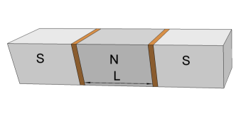
Figure 1: Schematic diagram of the SINIS junction

The influence of interfacial proximity effects in SINIS junctions on the phase relations, that results in a nonmonotonic dependence $\chi(\phi,L)$ at a fixed $L$, has not been identified in the literature until now.

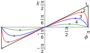
(a)

(b)

Figure 2: The internal phase difference $\chi$ (a) and the phase incursion $\varphi$ (b) as functions of the phase difference $\phi$ taken at various distances $l$:  (1)  $l=0.02$   (2)  $l=0.5$   (3)  $l=1.1$   (4)  $l=2.2$.

The relation was typically simplified assuming negligible values of either the phase incursion $\varphi$ over the central lead, or the phase drops $\chi$ across thin interfaces. More advanced earlier attempts of describing the SNS junction within the GL approach VolkovA1971 ; Fink1976 focused on the phase incursion and fully transparent interfaces, but were based on the specific boundary conditions and gave no consideration to the phase drops. Note1 On the other hand, microscopic theories of the double-junction systems, being elaborated on and applied to a wide temperature range down to zero temperature Kupriyanov1988 ; Kupriyanov1999 ; Golubov2000 ; Golubov2004 , usually assume a negligible current-induced phase incursion in contrast to the phase drops. While the latter point is justified for SISIS junctions in a wide range of realistic parameters, the range gets narrower in SINIS junctions, allowing both quantities $\chi$ and $\varphi$ to be of importance in the current transport at mesoscopic values of $L$, as shown below.

Description of the model.  Consider a symmetric tunnel SINIS junction with two identical thin interfaces set at distance $L$ on the side faces of the central normal metal lead (see Fig. 1). A one-dimensional spatial profile of the order parameter will establish itself in the system, if, for example, the electrodes’ transverse dimensions are much less than both the superconductor coherence length $\xi$ and the decay length $\xi_{n}$ in the central electrode. The system’s free energy involves the bulk and interface contributions ${\cal F}=\sum{\cal F}_{p}+{\cal F}_{n}+{\cal F}^{\text{int}}_{\frac{L}{2}}+{\cal F}^{\text{int}}_{-\frac{L}{2}}$. Here $p=1,2$ refer to the external superconducting electrodes, while subscript $n$ refers to the central normal metal lead. Assuming the latter to be described within the GL approach Note2 , one gets per unit area of the cross section

$$\!\!{\cal F}_{n}\!=\!\!\!\int\nolimits_{-L/2}^{L/2}\!\!\!dX\!\left[\!K_{n}\left|\dfrac{d}{dX}\Psi(X)\right|^{2}\!\!\!+a_{n}\left|\Psi(X)\right|^{2}\!\!+\dfrac{b_{n}}{2}\left|\Psi(X)\right|^{4}\right]\!,$$ (1)

where $K_{n},\,a_{n},\,b_{n}>0$ and the interfaces are placed at $X=\pm L/2$. The expressions for ${\cal F}_{1,2}$ are obtained from (1) after substituting $K_{n},\,a_{n},\,b_{n}\to K,\,-|a|,\,b$ and replacing the integration period $(-L/2,L/2)$ by $(-\infty,-L/2)$ or $(L/2,\infty)$ for $p=1$ or $2$, respectively.

The interfacial free energy per unit area is

$${\cal F}^{\text{int}}_{\pm\frac{L}{2}}\!=g_{J}\left|\Psi_{\pm\frac{L}{2}+}\!-\Psi_{\pm\frac{L}{2}-}\right|^{2}\!\!+g\left|\Psi_{\pm\frac{L}{2}\pm}\right|^{2}\!\!+g_{n}\left|\Psi_{\pm\frac{L}{2}\mp}\right|^{2}\!.$$ (2)

The first invariant in (2) describes the Josephson coupling while other terms take account of the interfacial pair breaking $g>0$, $g_{n}>0$.

The GL equation for the normalized absolute value of the order parameter in the central electrode $\Psi=(a_{n}/b_{n})^{1/2}fe^{\mathtt{i}\alpha}$ takes the form

$$\dfrac{d^{2}f}{dx^{2}}-\dfrac{i^{2}}{f^{3}}-f-f^{3}=0.$$ (3)

Here $x=X/\xi_{n}$, $\xi_{n}=(K_{n}/a_{n})^{1/2}$ and the dimensionless current density is $i=\frac{2}{3\sqrt{3}}(j\big{/}j_{\text{dp}})$, where $j_{\text{dp}}=\bigl{(}8|e|a_{n}^{3/2}K_{n}^{1/2}\bigr{)}\big{/}\bigl{(}3\sqrt{3}\hbar b_{n}\bigr{)}$.

The boundary conditions for the complex order parameter, which follow from (1) and (2), agree with the microscopic results Golubov2004 near $T_{c}$, at all transparency values Barash2012 ; Barash2012_2 ; Barash2014_3 . Introducing $l=L/\xi_{n}$, one gets, in particular:

$$\left(\dfrac{df}{dx}\right)_{l/2-0}\!\!=-\Bigl{(}g_{n,\delta}+g_{\ell}\Bigr{)}f_{-}+g_{\ell}\cos\chi f_{+},$$ (4)

$$i=-\,f^{2}\dfrac{d\alpha}{dx}=g_{\ell}f_{-}f_{+}\sin\chi.$$ (5)

Here $\chi\!=\!\alpha\left(\frac{l}{2}-0\right)\!-\!\alpha\left(\frac{l}{2}+0\right)$,  $f_{-}\!=\!f_{l/2-0}$,  $f_{+}\!=\!f_{l/2+0}$ and the dimensionless coupling constants $g_{\ell}\!=\!g_{J}\xi_{n}/K_{n}$, $g_{n,\delta}=g_{n}\xi_{n}/K_{n}$.

The phase relations. The proximity effect of the Josephson origin, associated with the term containing $\cos\chi$ in (4), takes place under the condition $g_{\ell}\cos\chi>0$, when the Josephson-coupling bilinear contribution to the free energy $\propto-2g_{\ell}f_{-}f_{+}\cos\chi$ decreases with an appearance of a small nonzero order parameter $f_{-}$ on one side of a thin interface, in the presence of $f_{+}$ on the other side. For $0$-junctions considered below $g_{\ell}>0$. Therefore, for superconductivity to appear in the central lead, the internal phase difference $\chi$ should change within the proximity-reduced range, $|\chi|\leq\chi_{\text{max}}(l)<\frac{\pi}{2}$, which is defined, in general, modulo $2\pi$. If $\chi$ were outside the range, the inverse proximity effect would prevent superconductivity to show up in the central lead.

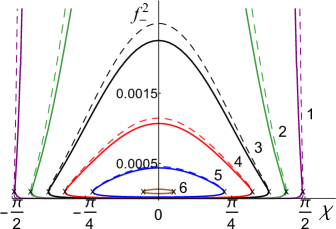
(a)

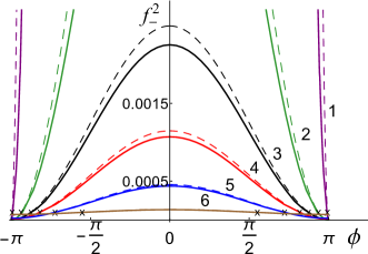
(b)

Figure 3: The quantity $f_{-}^{2}$ as (a) a double-valued function of $\chi$ and (b) a single-valued function of $\phi$ taken at various $l$:  (1)  $l=0.02$   (2)  $l=0.2$   (3)  $l=0.4$   (4)  $l=0.6$   (5)  $l=1$   (6)  $l=2.5$.

Figs. 2a and 2b show, respectively, the internal phase difference $\chi$ and the phase incursion $\varphi$, taken at various $l$ as functions of the phase difference $\phi$ between the superconductor terminals. All the numerical results have been obtained by carrying out an evaluation of the GL equations’ solutions that take into account the phase incursion and boundary conditions at interfaces with $g_{\ell}\!=\!g_{\delta}\!=\!0.01$ and $g_{n,\delta}\!=\!0$, assuming $K=K_{n}$, $|a|=a_{n}$ and $b=b_{n}$. ​The approximate analytical solutions for tunnel SINIS junctions have been also obtained. Note3 ​They describe almost perfectly the functions $\chi(\phi)$ and $\varphi(\phi)$ for the parameter set chosen, with deviations from the numerical results that are indiscernible in Figs. 2a and 2b.

If the phase incursion $\varphi$ is negligibly small, one gets from $\phi=2\chi+\varphi$ a simple dependence $\chi(\phi)=\frac{\phi}{2}$, which results in the variation range $|\chi|\leq\frac{\pi}{2}$ for $|\phi|\leq\pi$. Such a behavior takes place at sufficiently small distances $l\ll 1$, except for a narrow vicinity of $\phi=\pi$, as shown in the curves 1 in Figs. 2a and 2b. The curves 2-4 demonstrate that, in a wide range of $\phi$, $\chi$ is of importance at mesoscopic lengths $l\lesssim 1$, while a substantial influence of $\varphi$ on the phase relations appears at $l\gtrsim 1$.

Since the supercurrent is spatially constant due to the presumed quasi-one-dimensional character of the problem, a local decrease of the Cooper pair density is accompanied by the increase of the superfluid velocity, i.e., of the gradient of the order parameter phase. Therefore, small local values of $f$ result in a noticeable $\varphi$. Due to a spatial decay of the proximity-induced condensate density with increasing distances from the interfaces, $\varphi$ increases with $l$ at a given $\phi$, while the range of variation of $|\chi|\leq\chi_{\text{max}}(l)$ becomes smaller: $\chi_{\text{max}}(l)\approx\arccos(\tanh l)$. At $l\gg 1$ $f$ is especially small in the depth of the central electrode, $\varphi$ dominates the right-hand side in $\phi=2\chi+\varphi$, while $|\chi|$ is greatly reduced.

Fig. 2a demonstrates that $\chi$ is a nonmonotonic function of $\phi$ that passes through over the proximity-reduced region twice, there and back, while the phase difference $\phi$ between the superconducting terminals changes over the period. Two different values of $\phi$ at one and the same $\chi$ are linked to the different phase incursions and, more generally, to the two solutions of the GL equation for the absolute value of the order parameter, taken at a given $\chi$. The dots marked with crosses represent in all the figures the points of contact of the two solutions, i.e., indicate the corresponding quantities taken at $\chi=\pm\chi_{\text{max}}(l)$.

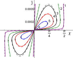
(a)

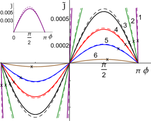
(b)

Figure 4: Normalized supercurrent as (a) a double-valued function of $\chi$ and (b) a single-valued function of $\phi$ taken at various $l$:   (1)  $l=0.02$   (2)  $l=0.2$   (3)  $l=0.4$   (4)  $l=0.6$   (5)  $l=1$   (6)  $l=2.5$.
Inset: The supercurrent at l=0.02 (solid line) and its analytical description at small $l$ (dashed line).

The order parameter $f_{-}$.   The nonlinear term $i^{2}f^{-3}\propto v_{s}^{2}(x)f(x)$ (where the superfluid velocity is $v_{s}(x)\propto i/f^{2}$) cannot, as a rule, be disregarded in (3) as compared to the linear one. In the depth of the central lead it dominates the latter, when $\phi$ is close to $\pi$. For this reason the GL equation (3) remains nonlinear even if the cubic term is negligible in the problem under consideration. As a result, there are two basic solutions for $f$ at a given $\chi$.

The normalized order-parameter absolute value squared $f^{2}_{-}$ taken at a side face of the central electrode is shown in Figs. 3a and 3b at various $l$ as a function of $\chi$ and $\phi$, respectively. The analytical description (dashed curves), that assumes the conditions $f_{-}\!\sim\!g_{\ell}f_{+}\!\ll\!1$ and $g_{n,\delta}\lesssim g_{\ell}$, approximates the numerical results shown reasonably well. As distinct from the phase relations in Fig. 2, the solid and dashed curves in Fig. 3 can be, mostly, clearly distinguished. The two solutions adjoin at $\chi\!=\!\pm\chi_{\text{max}}(l)$ and form the double-valued behavior shown in Fig. 3a. The first solution for $f_{-}$ has a maximum and the second one a minimum at $\chi\!=\!0$ at a fixed $l$. The same occurs at $l\to 0$ at a fixed $\chi$, where the minimum is zero.

If $\chi$ were fixed experimentally, the first solution would describe the stable and the second one the metastable states. However, the control parameter in experiments is usually $\phi$. After switching over from $\chi$ to $\phi$, the order parameter is described by the continuous single-valued dependence $f_{-}(\phi,l)$ shown in Fig. 3b. The first solution operates in the region $|\phi|\in(0,\phi_{*}(l))$ while the other one is in $|\phi|\in(\phi_{*}(l),\pi)$. Here $\phi_{*}(l)\approx\frac{\pi}{2}+\arcsin(\frac{1}{\cosh l})$. The adjoining regions do not overlap due to a substantial phase incursion occurring at small $f$. The curves’ crossing, seen in Fig. 3b at small $f_{-}$, is a manifestation of the opposite behavior of the two solutions with increasing $l$. If $\phi=\pi$, $f$ is zero at $x=0$ at arbitrary $l$, that allows phase-slip processes in the central lead. Fink1976 ; Giazotto2017 ; Note3

For tunnel interfaces one obtains $f_{-}\sim g_{\ell}f_{+}\ll 1$ at $g_{n,\delta}\lesssim g_{\ell}$, except for the first solution at sufficiently small $l$. The latter results, in the limit $l\to 0$, in the relation $f_{-}\!=\!\frac{g_{\ell}\cos\chi}{g_{\ell}+g_{n,\delta}}f_{+}$, which also applies to SISIS junctions Barash2018 and approximately describes the dependence on $\chi$. For the whole parameter set used in the figures $f_{+}$ weakly changes with $\chi$ and $l$: $f_{+}^{2}\in(0.972,0.978)$. If $g_{n,\delta}\lesssim g_{\ell}$ and $\cos\chi\sim 1$, one obtains $f_{-}\sim f_{+}$, while in the opposite case $g_{n,\delta}\gg g_{\ell}$ the relation is $f_{-}\ll f_{+}$. Since $g_{\ell}$ for tunnel interfaces is proportional to the transmission coefficient $g_{\ell}\propto{\cal D}$ Barash2012 ; Barash2012_2 ; Barash2014_3 , the above relation results in $f_{-}\propto{\cal D}$, if $g_{\ell}\ll g_{n,\delta}$, and in the ${\cal D}$-independent quantity $f_{-}$ for $g_{\ell}\gg g_{n,\delta}$. The second solution vanishes in the limit $l\to 0$, and satisfies the relation $f_{-}=g_{\ell}f_{+}\tanh\frac{l}{2}$ at arbitrary $l$ and $\chi=0$. In the case of large $l$ the two solutions coincide and the relation at $\chi=0$ is $f_{-}=g_{\ell}f_{+}$. Note3

The supercurrent.  The normalized supercurrent $\tilde{\jmath}=j\big{/}j_{\text{dp}}$ is depicted in Figs. 4a and 4b at various $l$ as a function of $\chi$ and $\phi$, respectively.​​ With respect to $\chi$, the supercurrent is in the shape of a double loop that looks like a sloping figure eight composed of the two solutions. After switching over from $\chi$ to $\phi$ the current-phase relation acquires the conventional form. The dashed curves, that correspond to approximate analytical results Note3 , have the sinusoidal shape in Fig. 4b. They deviate within several percent from the numerical results (solid curves).

A substantial role of the phase incursion in creating such a behavior can be understood as follows. The supercurrent $\propto g_{\ell}f_{-}f_{+}\sin\chi$ is influenced by the proximity effect together with $f_{-}$. If $\varphi$ were completely neglected, the value $\phi\!=\!\pi$ would correspond to $\chi\!=\!\frac{\pi}{2}$. Since the proximity effect vanishes at $\chi\to\frac{\pi}{2}$, one gets $f_{-}\!\!\to 0$ that could explain the zeroth supercurrent at $\phi=\pi$. However, as $f_{-}$ is small in the vicinity of $\phi=\pi$, one gets a noticeable phase incursion that reduces the variation range $|\chi|\leq\chi_{\text{max}}(l)<\frac{\pi}{2}$ and excludes a possibility for $\chi$ to reach $\frac{\pi}{2}$ at any nonzero $l$. Instead, there appear two solutions of the GL equation providing a return passage for $\chi$, from $0$ to $\chi_{\text{max}}(l)$ and back, while $\phi$ changes over $(0,\pi)$. As a result, the correspondence of $\chi=0$ to both $\phi=0$ and $\phi=\pi$ is established. The phase relations in the SINIS systems do not result in the regime of interchanging modes with abrupt supercurrent changes, that can occur in SISIS junctions. Luca2009 ; Linder2017 ; Barash2018

The small values of the order parameter and supercurrent, that are characteristic for the second solution and marked with crosses in Figs. 3 and 4, are specifically associated with the choice $g_{\ell}=0.01$ for the Josephson coupling constant, taken for demonstrating a quantitative agreement between the numerical and approximate analytical results. The effects discussed increase with $g_{\ell}$ and remain qualitatively the same for $g_{\ell}\lesssim 1$. Note4 Thus for $g_{\ell}=0.1$ instead of $g_{\ell}=0.01$, the characteristic values of $f_{-}^{2}$ and $\tilde{\jmath}$ increase in about $50-100$ times.

The first solution is strongly modified at small distances $l\lesssim 2g_{\ell}(b_{n}|a|/ba_{n})^{1/2}\ll 1$, for which the analytical description, based on the relation $f_{-}=\frac{g_{\ell}\cos\chi}{g_{\ell}+g_{n,\delta}}f_{+}$ rather than on $f_{-}\sim g_{\ell}f_{+}\ll 1$, has to be developed. Note3 The inset in Fig. 4b shows the solid curve 1 as a whole ($l=0.02$). The analytical results deviate weakly from the solid curve. When $g_{n,\delta}\ll g_{\ell}$, one obtains $j\propto{\cal D}$. A remarkable feature is that the supercurrent dependence on the transparency gradually evolves into ${\cal D}^{2}$ with increasing $\phi$ up to about $\phi_{*}$ at a fixed small $l$, due to the increase of the phase incursion with $\phi$. Similar supercurrent behavior also takes place for some other reasons, in particular, with the increasing distance $l$. Kupriyanov1988 ; Kupriyanov1999 ; Golubov2000 ; Golubov2004 For the second solution one always obtains $j\propto{\cal D}^{2}$. Such a crossover is a fingerprint of the underlying physics associated with the phase-dependent proximity effect of the Josephson origin that generates the unconventional behavior of internal phase differences in SINIS junctions.

The research is carried out within the state task of ISSP RAS.

Two symmetric one-dimensional solutions to the GL equation are analytically described for tunnel SINIS junctions with the parameters linked by the boundary and asymptotic conditions.

S1 Symmetric solutions to the GL equation

The GL equation for the absolute order-parameter value can be written as

$$\left\{\begin{aligned} &\dfrac{d^{2}f}{dx^{2}}-\dfrac{i^{2}}{f^{3}}-f-f^{3}=0,\quad|x|<l/2,\\ \\ &\dfrac{d^{2}f}{dx^{2}}-\dfrac{K_{n}^{2}}{K^{2}}\cdot\dfrac{i^{2}}{f^{3}}+\dfrac{|a|K_{n}}{a_{n}K}f-\dfrac{bK_{n}}{b_{n}K}f^{3}=0,\quad|x|>l/2.\end{aligned}\right.$$ (S1)

Here the dimensionless quantities $f$ and $x$ are defined as $\Psi\!=\!(a_{n}/b_{n})^{1/2}fe^{\mathtt{i}\alpha}$, $x\!=\!X/\xi_{n}$. Also $l\!=\!L/\xi_{n}$, $\xi_{n}\!\!=\!(K_{n}/a_{n})^{1/2}$ and the dimensionless current density is $i\!=\!\frac{2}{3\sqrt{3}}(j\big{/}j_{\text{dp}})$, where $j_{\text{dp}}\!=\!\bigl{(}8|e|a_{n}^{3/2}K_{n}^{1/2}\bigr{)}\big{/}\bigl{(}3\sqrt{3}\hbar b_{n}\bigr{)}$. One also assumes $a_{n}\sim|a|$ that makes possible a joint description of the normal metal and superconducting leads within the GL approach. SAbrikosov1988

The boundary conditions at the interfaces at $x=\pm l/2$ take the form

$$\left\{\begin{aligned} &\left(\dfrac{df}{dx}\right)_{\pm(l/2-0)}=\mp\bigl{(}g_{n,\delta}+g_{\ell}\bigr{)}f_{-}\pm g_{\ell}f_{+}\cos\chi,\\ &\dfrac{K}{K_{n}}\left(\dfrac{df}{dx}\right)_{\pm(l/2+0)}=\pm(g_{\delta}+g_{\ell})f_{+}\mp g_{\ell}f_{-}\cos\chi,\end{aligned}\right.$$ (S2)

where the dimensionless coupling constants are $g_{\ell}\!=\!g_{J}\xi_{n}(T)/K_{n}$, $g_{n,\delta}=g_{n}\xi_{n}(T)/K_{n}$ and the symmetric solutions $f(x)=f(-x)$ are considered.

The Josephson current described by the relation (5) of the main text can also be expressed via the asymptotic absolute value $f_{\infty}$ of the superconductor order parameter:

$$i^{2}=\dfrac{Kb}{K_{n}b_{n}}\left(\dfrac{|a|b_{n}}{a_{n}b}-f_{\infty}^{2}\right)f_{\infty}^{4}.$$ (S3)

In the absence of the supercurrent one gets, for the normalization chosen,

$$f_{\infty}^{2}=\frac{|a|b_{n}}{a_{n}b}.$$ (S4)

Equating (5) and (S3) results in the equation

$$\dfrac{Kb}{K_{n}b_{n}}\left(\dfrac{|a|b_{n}}{a_{n}b}-f_{\infty}^{2}\right)f_{\infty}^{4}=g_{\ell}^{2}f_{-}^{2}f_{+}^{2}\sin^{2}\chi.$$ (S5)

Symmetric analytical solutions to the GL equations (S1) describe the order-parameter absolute value that satisfies the boundary conditions (S2) at the thin interfaces, as well as the asymptotic conditions (S4) deep inside the long superconductor leads. The energetically most favorable solutions are expected to describe the proximity-induced order parameter absolute value in the normal metal lead with a single minimum at the center $x=0$ between the interfaces and the equal maximums $f_{-}$ at the side faces of the central electrode $x=\pm(l/2-0)$. In each of the external leads, the order parameter has its maximum $f_{\infty}$ at asymptotically large distances and minimum $f_{+}$ at pair breaking boundaries $x=\pm(l/2+0)$. The parameters $f_{\pm}$ and $f_{\infty}$ depend on the phase difference $\chi$ and the central lead’s length $l$ and should be determined together with other parameters of the whole solution.

For obtaining the solutions, the first integral of (S1) will be used. The corresponding quantities ${\cal E}_{n}$ and ${\cal E}$, defined as

$${\cal E}_{n}=\!\left(\dfrac{df(x)}{dx}\right)^{2}\!\!\!+\dfrac{i^{2}}{f^{2}(x)}-f^{2}(x)-$$

$$\qquad\qquad\qquad\qquad\qquad-\dfrac{1}{2}f^{4}(x),\enspace|x|<l/2,$$ (S6)

$${\cal E}=\left(\dfrac{df(x)}{dx}\right)^{2}+\dfrac{K_{n}^{2}}{K^{2}}\dfrac{i^{2}}{f^{2}(x)}+\dfrac{|a|K_{n}}{a_{n}K}f^{2}(x)-$$

$$\qquad\qquad\qquad\qquad-\dfrac{bK_{n}}{2b_{n}K}f^{4}(x),\enspace|x|>l/2,$$ (S7)

are spatially constant, when taken for the solutions to (S1) inside the central electrode and the external leads, respectively. Since the boundary conditions (S2) do not generally support the conservation of ${\cal E}$ through the interfaces, ${\cal E}_{n}$ and ${\cal E}$ can substantially differ from each other.

Eq. (S6) can be rewritten in the form

$$\left(\dfrac{dt}{dx}\right)^{2}=2(t-t_{1})(t-t_{2})(t-t_{3}),\enspace|x|<l/2,$$ (S8)

where $t(x)\equiv f^{2}(x)$.

The quantities $t_{i}=f_{i}^{2}$, $i=1,2,3$ satisfy the following set of equations

$$t_{1}+t_{2}+t_{3}=-2,\enspace t_{1}t_{2}t_{3}=2i^{2},\enspace t_{1}t_{2}+t_{1}t_{3}+t_{2}t_{3}=2{\cal E}_{n}.$$ (S9)

Solutions to equation (S8) are characterized by three formal extrema $t_{1},\,t_{2},\,t_{3}$ with the vanishing first derivative $\frac{dt}{dx}$. In general, either all three roots $t_{1},\,t_{2}$ and $t_{3}$ take on real values, or only one is real and two are the complex conjugate of each other. As the numerical study shows, only real values of $t_{i}$ are relevant for the given problem. For superconducting leads real roots usually take nonnegative values $t_{i}\geq 0$ ($i=1,2,3$). SBarash2017 ; SBarash2018 For the proximity influenced normal metal lead only one of the real roots is nonnegative:  $t_{1}\geq 0$,  $t_{2,3}\leq 0$, as ensured by the sign minus and sign plus on the right hand sides of the first and second equations in (S9), respectively. The sign minus originates from the condition $a_{n}>0$ for the normal metal. For the superconducting lead $a<0$, that would result in the sign plus instead of minus.

As the left hand side of (S8) takes on nonnegative values, the quantity $t_{1}$ has to be the minimum. While the negative roots $t_{2,3}$ correspond to purely imaginary quantities $f_{2,3}$, $t_{1}$ just represents the actual minimum that $t(x)=f^{2}(x)$ takes at the central point of the normal metal lead $x=0$.

Thus, the solution inside the central lead $|x|<l/2$ should monotonically increase with $|x|$ and, in particular, have a nonnegative derivative at $x=l/2-0$. As follows from (S2), the latter conditions require $-\bigl{(}g_{n,\delta}+g_{\ell}\bigr{)}\sqrt{t_{-}}+g_{\ell}\cos\chi\sqrt{t_{+}}\geq 0$ and $t_{3}\leq t_{2}\leq 0\leq t_{1}\leq t(x)\leq t_{-}\leq t_{+}$. In accordance with the above, one gets from Eq. (S8):

$$|x(t)|=\sqrt{\dfrac{2}{t_{1}-t_{3}}}F\left(\left.\arcsin\sqrt{\frac{t-t_{1}}{t-t_{2}}}\,\right|\,\frac{t_{2}-t_{3}}{t_{1}-t_{3}}\right).$$ (S10)

Here the definitions of the Mathematica book are used for the notations of arguments of the elliptic integral of the first kind $F\left(\varphi\left|\,m\right.\right)$. SWolfram2003

Taking $x=l/2-0$ in (S10) results in the condition associated with the central lead’s length:

$$\sqrt{\dfrac{2}{t_{1}-t_{3}}}F\!\left(\left.\arcsin\sqrt{\frac{t_{-}-t_{1}}{t_{-}-t_{2}}}\,\right|\,\frac{t_{2}-t_{3}}{t_{1}-t_{3}}\right)=\dfrac{l}{2}.$$ (S11)

The quantity ${\cal E}_{n}$ for the central lead can be expressed via $t_{\pm}$, taking $x=(l/2)-0$ in (S6) and making use of (5) and the first equation in (S2):

$${\cal E}_{n}=\biggl{[}-1+\Bigl{(}g_{n,\delta}+g_{\ell}\Bigr{)}^{2}\biggr{]}t_{-}+g_{\ell}^{2}t_{+}-\\ -2g_{\ell}\Bigl{(}g_{\ell}+g_{n,\delta}\Bigr{)}\cos\chi\sqrt{t_{-}t_{+}}-\dfrac{1}{2}t_{-}^{2}\,.$$ (S12)

Taking $x\to\infty$ in (S7) and using (S3), one obtains

$${\cal E}=\dfrac{bK_{n}}{b_{n}K}\left(2\dfrac{|a|b_{n}}{a_{n}b}-\dfrac{3}{2}t_{\infty}\right)t_{\infty}.$$ (S13)

On account of (S3) and (S13), equation (S7) can be rewritten in the form

$$\left(\dfrac{dt}{dx}\right)^{2}=\dfrac{2K_{n}b}{Kb_{n}}\bigl{(}t_{\infty}-t\bigr{)}^{2}\left(t-2\left(\dfrac{|a|b_{n}}{a_{n}b}-t_{\infty}\right)\right).$$ (S14)

The nonnegative value of the left hand side in (S14) requires the solution $t(x)$ to satisfy the condition $t\geq 2\left(\dfrac{|a|b_{n}}{a_{n}b}-t_{\infty}\right)$ in the external region $|x|>l/2$.

Taking the square root of both sides of (S14) at $x=l/2+0$ and substituting the result in the second boundary condition in (S2), one excludes the derivative of the order parameter absolute value, taken at the boundary, and obtains

$$\left(t_{\infty}-t_{+}\right)\sqrt{2t_{\infty}+t_{+}-2\frac{|a|b_{n}}{a_{n}b}}=\\ =\sqrt{\dfrac{2K_{n}b_{n}}{Kb}}\left[\Bigl{(}g_{\delta}+g_{\ell}\Bigr{)}t_{+}-g_{\ell}\cos\chi\sqrt{t_{-}t_{+}}\right].$$ (S15)

Positive sign of the left hand side in (S15) entails the relation $\Bigl{(}g_{\delta}+g_{\ell}\Bigr{)}\sqrt{t_{+}}>g_{\ell}\cos\chi\sqrt{t_{-}}$.

Since the supercurrent is expressed in (5) via the quantities $t_{\pm}$, the analysis of the full spatial order parameter profile can be omitted here. However, one needs to study the external phase difference $\phi=2\chi+\varphi$ and the associated phase incursion $\varphi$.

For the gradient of the order parameter phase one gets from (5)

$$\dfrac{d\alpha}{dx}=-\,\dfrac{i}{f^{2}}.$$ (S16)

Integrating both sides in (S16) along the central lead and using (S8), one has

$$\varphi=\sqrt{2}i\!\!\int\limits_{t_{1}}^{t_{-}}\!\!\dfrac{dt}{t\sqrt{(t-t_{1})(t-t_{2})(t-t_{3})}},$$ (S17)

where $\varphi=\alpha(-l/2+0)-\alpha(l/2-0)$. After taking into account the relation (S11), the result of the integration in (S17) contains the elliptic integral of the third kind and takes the form

$$\varphi=\frac{2i}{t_{2}}\Biggl{[}-\,\dfrac{\sqrt{2}(t_{1}-t_{2})}{t_{1}\sqrt{t_{1}-t_{3}}}\,\Pi\!\left(\frac{t_{2}}{t_{1}-t_{2}};\arcsin\sqrt{\frac{t_{-}-t_{1}}{t_{-}-t_{2}}}\left|\frac{t_{2}-t_{3}}{t_{1}-t_{3}}\right.\right)+\frac{l}{2}\Biggr{]}.$$ (S18)

The solutions to Eqs. (S1) have to satisfy the relation (S11), the boundary and asymptotic conditions. As a result, the full parameter set contains six quantities $t_{1}$, $t_{2}$, $t_{3}$, $t_{\pm}$, and $t_{\infty}$, which are linked to each other by six equations (S9), (S11), (S15) and (S5), where expressions (S12) and (5) should be substituted for ${\cal E}_{n}$ and $i$. Joint solutions to the equations studied represent the parameters as functions of the phase difference $\chi$ and the dimensionless length $l$ of the central lead. Though the numerical study of such solutions is generally required, a number of important problems allow analytical descriptions. Both approaches demonstrate the presence of two solutions that satisfy the above equations. The analytical solutions will be presented in the following sections.

S2 Exact results at $\chi=0$

The description of currentless states in the SINIS junctions can be analytically reduced, for each of the solutions, to a comparatively simple exact relation between $l$ and $t_{-}$. As it follows from (5) and (S3), for the currentless states $\chi=0$ and $t_{\infty}=\frac{|a|b_{n}}{a_{n}b}$. With this $\chi$ and $t_{\infty}$, one gets from (S15) the expression for $f_{+}\equiv\sqrt{t_{+}}$ as a function of $f_{-}\equiv\sqrt{t_{-}}$:

$$f_{+}(f_{-})=\sqrt{\dfrac{|a|b_{n}}{a_{n}b}+\dfrac{K_{n}b_{n}}{2Kb}(g_{\delta}+g_{\ell})^{2}+\sqrt{\dfrac{2K_{n}b_{n}}{Kb}}g_{\ell}f_{-}}-\\ -\sqrt{\dfrac{K_{n}b_{n}}{2Kb}}(g_{\delta}+g_{\ell}).$$ (S19)

Taking $\chi=0$ in (S9), (S11), where $i=0$ and ${\cal E}_{n}$ is defined in (S12), one obtains two solutions. The first solution corresponds to ${\cal E}_{n}\leq 0$ and $\phi=0$, while the second one describes the case ${\cal E}_{n}\geq 0$ and $\phi=\pi$.

For the first solution at $\chi=\phi=0$ one obtains $t_{2}=0$. Substituting $t_{2}=0$ in (S9), results in

$$t_{1,3}(t_{-})=-1\pm\sqrt{1-2{\cal E}_{n}}=\\ =-1\pm\sqrt{(1+f_{-}^{2})^{2}-2[(g_{n,\delta}+g_{\ell})f_{-}-g_{\ell}f_{+}(t_{-})]^{2}},$$ (S20)

where

$${\cal E}_{n}=-t_{-}-\dfrac{1}{2}t_{-}^{2}+\Bigl{[}g_{\ell}f_{+}-(g_{\ell}+g_{n,\delta})f_{-}\Bigr{]}^{2}.$$ (S21)

It follows from (S20) and the condition ${\cal E}_{n}\!\leq 0$ that $t_{1}\!>\!0$.

The basic dependence $l(t_{-})$, that follows from (S11) for the first solution at $\chi=\phi=0$, is

$$l_{+}(t_{-})=\dfrac{2\sqrt{2}}{\sqrt{t_{1}-t_{3}}}F\!\left(\left.\arcsin\sqrt{1-\frac{t_{1}}{t_{-}}}\,\right|\,\frac{|t_{3}|}{t_{1}+|t_{3}|}\right),$$ (S22)

where the expressions (S19)-(S21) define $t_{1,3}\equiv f_{1,3}^{2}$ as a function of $t_{-}$.

For the second solution, at $\chi=0$ and $\phi=\pi$, one obtains $t_{1}=0$. With $t_{1}=0$ one gets from (S9)

$$t_{2,3}(t_{-})=-1\pm\sqrt{1-2{\cal E}_{n}}=\\ =-1\pm\sqrt{(1+f_{-}^{2})^{2}-2[(g_{n,\delta}+g_{\ell})f_{-}-g_{\ell}f_{+}(t_{-})]^{2}},$$ (S23)

It follows from (S23) and the condition ${\cal E}_{n}\geq 0$ that both quantities $t_{2,3}\leq 0$.

The basic dependence $l(t_{-})$, that follows from (S11) for the second solution at $\chi=0$ and $\phi=\pi$, is

$$l_{-}(t_{-})=\dfrac{2\sqrt{2}}{\sqrt{|t_{3}|}}F\!\left(\left.\arcsin\sqrt{\frac{t_{-}}{t_{-}+|t_{2}|}}\,\right|\,\frac{|t_{3}|-|t_{2}|}{|t_{3}|}\right),$$ (S24)

where the expressions (S19) and (S23) define $t_{2,3}\equiv f_{2,3}^{2}$ as the functions of $t_{-}$.

For the first solution, the quantity $t_{-}(l)$, described by (S22), is a monotonically decreasing function of $l$, while the second solution (S24) monotonically increases with $l$. The value $t_{-}$ in the limit $l\to 0$ is determined for the first solution (S22) by the equality $t_{-}=t_{1}$. The latter immediately results in the relation

$$f_{-}=\frac{g_{\ell}}{g_{\ell}+g_{n,\delta}}f_{+}.$$ (S25)

For the second solution, one finds from (S24) $t_{-}=0$ in the limit $l\to 0$.

The limiting case $l\to\infty$ corresponds to $t_{1}=0$ in (S22), and to $t_{2}=0$ in (S24). The conditions are equivalent in both cases and take the form

$${\cal E}_{n}(f_{-})=0,$$ (S26)

where (S19) should be substituted for $f_{+}$ in (S21). The numerical studies confirm the above conclusions.

S3 Solutions at small distances

The solution of the problem considered can be analytically obtained within the zeroth-order approximation in a small parameter $l$. The first argument of the elliptic integral in (S11) should vanish in this case and, therefore, $t_{1}=t_{-}$. Taking account of the latter equality in (S9) results in

$$t_{2}+t_{3}= -\left(2+t_{-}\right),\quad t_{-}(t_{2}+t_{3})+t_{2}t_{3}=2{\cal E}_{n},$$

$$t_{-}t_{2}t_{3}=2g_{\ell}^{2}t_{-}t_{+}\sin^{2}\chi.$$ (S27)

In the limit $l\to 0$ the SINIS system is in some aspects similar to symmetric SISIS junctions, and the present section generalizes the results of Appendix C in Ref. SBarash2018, to the case, when different normalizations in the central and external leads are preferable under different conditions.

There are two solutions to the system of equations (S27). The first solution is obtained, assuming $t_{-}\neq 0$ and using (S12) and (5), and results in the relation

$$f_{-}=\dfrac{g_{\ell}\cos\chi}{g_{n,\delta}+g_{\ell}}f_{+},$$ (S28)

which is in agreement with the exact result (S25) at $\chi=0$. The condition $g_{\ell}\cos\chi>0$, required for $f_{-}>0$ in (S28), ensures the presence of the proximity effect of the Josephson origin.

Substituting (S28) for $f_{-}$ in (5) and in the second boundary condition in (S2), taken at $x=l/2+0$, allows one to incorporate the quantities describing the central electrodes into the effective characteristics of the united interface with boundaries at $x=\pm(l/2+0)$ in a single symmetric Josephson junction. With the phase incursion over the central lead neglected in the limit $l\to 0$, the first solution results in

$$i=g_{\ell}^{\text{eff}}f_{+}^{2}\sin\phi,\quad g_{\ell}^{\text{eff}}=\dfrac{g_{\ell}^{2}}{2(g_{n,\delta}+g_{\ell})}$$ (S29)

and in the following equality

$$\dfrac{K}{K_{n}}\left(\dfrac{df}{dx}\right)_{l/2+0}\!\!\!=\biggl{[}\dfrac{g_{\delta}g_{n,\delta}+g_{\ell}(g_{\delta}+g_{n,\delta})}{g_{n,\delta}+g_{\ell}}+\\ +2\dfrac{g_{\ell}^{2}}{2\left(g_{n,\delta}+g_{\ell}\right)}\sin^{2}\dfrac{\phi}{2}\biggr{]}f_{+}\,.$$ (S30)

The central electrode has mainly been the focus of the study until now, and all the quantities have been normalized with respect to the central electrode’s characteristics. Since the external superconductor electrodes have taken the priority at the moment, it will be convenient to switch over to the normalization based on their properties. One introduces

$$\tilde{f}=\sqrt{\dfrac{a_{n}b}{|a|b_{n}}}f, \tilde{x}=\sqrt{\dfrac{K_{n}|a|}{Ka_{n}}}x, \tilde{l}=\sqrt{\dfrac{K_{n}|a|}{Ka_{n}}}l,$$

$$\tilde{g}_{\ell}=\sqrt{\dfrac{K_{n}a_{n}}{K|a|}}g_{\ell}, \tilde{g}_{\delta}=\sqrt{\dfrac{K_{n}a_{n}}{K|a|}}g_{\delta}, \tilde{g}_{n,\delta}=\sqrt{\dfrac{K_{n}a_{n}}{K|a|}}g_{n,\delta}.$$ (S31)

and obtains from (S30)

$$\left(\dfrac{d\tilde{f}}{d\tilde{x}}\right)_{\tilde{l}/2+0}\!\!\!=\biggl{[}\dfrac{\tilde{g}_{\delta}\tilde{g}_{n,\delta}+\tilde{g}_{\ell}(\tilde{g}_{\delta}+\tilde{g}_{n,\delta})}{\tilde{g}_{n,\delta}+\tilde{g}_{\ell}}+\\ +2\dfrac{\tilde{g}_{\ell}^{2}}{2\left(\tilde{g}_{n,\delta}+\tilde{g}_{\ell}\right)}\sin^{2}\dfrac{\phi}{2}\biggr{]}\tilde{f}_{+}\,.$$ (S32)

Equation (S32) is of the form of the boundary condition for the order-parameter absolute value in a single symmetric Josephson junction with the phase difference $\phi$ across the interface SBarash2012 ; SBarash2014_3

$$\left(\dfrac{d\tilde{f}}{dx}\right)_{l/2+0}=\Bigl{(}\tilde{g}_{\delta}^{\text{eff}}+2\tilde{g}_{\ell}^{\text{eff}}\sin^{2}\dfrac{\phi}{2}\Bigr{)}\tilde{f}_{l/2+0}.$$ (S33)

Therefore, the problem of the SINIS junction reduces in the limit $l\to 0$ to the behavior of a single Josephson junction, described by the first solution. The Josephson current flowing through a single junction is known in the GL theory in detail at any coupling constants’ values. Here the effective constants of the Josephson coupling and the interfacial pair breaking are associated with the characteristics of the SINIS junction. The quantity $g_{\ell}^{\text{eff}}$ is defined in (S29), and $g_{\delta}^{\text{eff}}$ takes the form

$$g_{\delta}^{\text{eff}}=\dfrac{g_{\delta}g_{n,\delta}+g_{\ell}(g_{\delta}+g_{n,\delta})}{g_{n,\delta}+g_{\ell}}.$$ (S34)

Changing the normalization will not modify the form of the effective coupling-constants’ definitions.

The second solution of the system (S27) describes, in the limit $l\to 0$, the superconducting external leads and the normal metal state in the central electrode: $t_{1}\!=\!t_{-}\!=\!0$, $i\!=\!0$, ${\cal E}_{n}\!=\!g_{\ell}^{2}t_{+}$, $t_{\infty}\!=\!\frac{|a|b_{n}}{a_{n}b}$, $t_{2,3}=-1\pm\sqrt{1-2g_{\ell}^{2}t_{+}}$,

$$t_{+}=\!\biggl{(}\!\sqrt{\frac{|a|b_{n}}{a_{n}b}+\frac{K_{n}b_{n}}{2Kb}(g_{\delta}+g_{\ell})^{2}}-\sqrt{\frac{K_{n}b_{n}}{2Kb}}(g_{\delta}+g_{\ell})\!\biggr{)}^{2}\!.$$ (S35)

The solution does not contain any phase dependence as no superconductivity is present in the central electrode.

S4 Solutions with small $f_{-}$ for tunnel interfaces

The analytical solutions to the GL equation can be found assuming $f_{-}\sim g_{\ell}f_{+}\ll 1$ and $g_{n,\delta}\lesssim g_{\ell}$. The former condition makes possible to disregard the cubic term in the first GL equation in (S1), as compared to the linear one:

$$\dfrac{d^{2}f}{dx^{2}}-\dfrac{i^{2}}{f^{3}}-f=0,\quad|x|<l/2.$$ (S36)

The solution to this equation is

$$f(x)=\sqrt{t_{1}\cosh^{2}x-t_{2}\sinh^{2}x},$$ (S37)

where the parameters $t_{1}\geq 0$ and $t_{2}\leq 0$ satisfy

$$t_{1}t_{2}=-i^{2},\quad t_{1}+t_{2}=-{\cal E}_{n}.$$ (S38)

The absolute value of the order parameter inside the central lead has the maximums $f_{-}$ at its side faces $x=\pm l/2$ and the minimum $f_{1}$ at its center $x=0$.

Assuming $g_{\ell}f_{+}$ and $f_{-}$ to be the quantities of the same order of smallness, one can satisfy the relation $f_{-}\gg 2g_{\ell}(g_{\ell}+g_{n,\delta})f_{+}$ and reduce the expression (S12) for ${\cal E}_{n}$ to the following simplified form

$${\cal E}_{n}=-t_{-}+g_{\ell}^{2}t_{+}.$$ (S39)

Using (S37)-(S39) and (5), one gets the system of equations

$$t_{1}t_{2}=-g^{2}_{\ell}t_{-}t_{+}\sin^{2}\chi_{r},$$

$$t_{1}+t_{2}=t_{-}-g^{2}_{\ell}t_{+},$$

$$t_{-}=t_{1}\cosh^{2}\frac{l}{2}-t_{2}\sinh^{2}\frac{l}{2},$$ (S40)

where the quantities $t_{-}$, $t_{1,2}$ are on the order of $g^{2}_{\ell}t_{+}$, with the higher order terms disregarded.

There are two solutions to (S40):

$$f_{-,\pm}=g_{\ell}f_{+}\coth l\biggl{[}\cos\chi\pm\sqrt{\cos^{2}\chi-\tanh^{2}l}\,\biggr{]},$$ (S41)

$$t_{1,\pm}=\frac{1}{2}g^{2}_{\ell}t_{+}\biggl{\{}-2+\biggl{(}1+\coth^{2}\frac{l}{2}\biggr{)}\cos\chi\biggl{[}\cos\chi\pm\sqrt{\cos^{2}\chi-\tanh^{2}l}\,\biggr{]}\biggr{\}},$$ (S42)

$$t_{2,\pm}=\frac{1}{2}g^{2}_{\ell}t_{+}\biggl{\{}-2+\biggl{(}1+\tanh^{2}\frac{l}{2}\biggr{)}\cos\chi\biggl{[}\cos\chi\pm\sqrt{\cos^{2}\chi-\tanh^{2}l}\,\biggr{]}\biggr{\}},$$ (S43)

taking place under the condition

$$|\chi|\leq\chi_{\text{max}}(l)=\arccos\tanh l.$$ (S44)

Within the same approximation one obtains that the last term on the right hand side in (S15) can be disregarded and $f_{\infty}$ coincides with its currentless value. The results can be represented as

$$\tilde{f}_{\infty}=1,\quad\tilde{f}_{+}=1-\dfrac{1}{\sqrt{2}}(\tilde{g}_{\delta}+\tilde{g}_{\ell}),$$ (S45)

where the normalization defined in (S31) is used. Since $t_{+}$ should be taken in (S41)-(S43) within the zeroth approximation in $g_{\ell}$, one has $t_{+}^{(0)}=\frac{b_{n}|a|}{ba_{n}}$.

The quantity $f_{-,+}(\chi,l)$, i.e., the first solution for $f_{-}$ in (S41) taken at the side face, has its maximum at $\chi=0$ and minimum at $\chi=\pm\chi_{\text{max}}(l)$. At the same time, the second solution $f_{-,-}(\chi,l)$ for $f_{-}$ has its maximum at $\chi=\chi_{\text{max}}(l)$ and minimum at $\chi=0$:

$$f_{-,+}(0,l)=g_{\ell}\coth\frac{l}{2}\left(\frac{b_{n}|a|}{ba_{n}}\right)^{1/2},$$ (S46)

$$f_{-,-}(0,l)=g_{\ell}\tanh\frac{l}{2}\left(\frac{b_{n}|a|}{ba_{n}}\right)^{1/2},$$ (S47)

$$f_{-,\pm}(\chi_{\text{max}}(l),l)=g_{\ell}\left(\frac{b_{n}|a|}{ba_{n}}\right)^{1/2}.$$ (S48)

It is worth noting that the quantity $f_{-,\pm}(\chi_{\text{max}}(l),l)$ does not depend on $l$ within the approximation used. The limiting behavior $f_{-,-}(0,l)\to 0$ at $l\to 0$ agrees with the exact result (S24) and the second solution in Sec. S3.

Substituting the maximal order parameter value (S46) in the presumed condition $f_{-}\ll 1$, one finds that the first solution in (S37), (S41)-(S43), taken at $\cos\chi\sim 1$, is justified when the length of the central lead is not too small: $l\gg 2g_{\ell}\left(\frac{b_{n}|a|}{ba_{n}}\right)^{1/2}$. For the parameter set used in the main text in plotting the figures, one gets $l\gg 0.02$. At sufficiently small $l$ and $\cos\chi\sim 1$ the first solution has been considered in the preceding section. At the same time, the results obtained in this section can be well applied at any $l$ to the second solution, as well as to the first one in a vicinity of $\chi=\chi_{\text{max}}(l)$.

For the absolute order parameter value $f_{1}$, at the center of the normal metal lead $x=0$, one finds from (S42):

$$f_{1,+}(0,l)=\dfrac{g_{\ell}}{\sinh\frac{l}{2}}\left(\frac{b_{n}|a|}{ba_{n}}\right)^{1/2},$$ (S49)

$$f_{1,-}(0,l)=0,$$ (S50)

$$f_{1,\pm}(\chi_{\text{max}}(l),l)=\dfrac{g_{\ell}}{\sqrt{\cosh l}}\left(\frac{b_{n}|a|}{ba_{n}}\right)^{1/2}.$$ (S51)

The most interesting point regarding $f_{1}$ is the vanishing second solution at $\chi=0$. In other words, in agreement with earlier results SFink1976 ; SGiazotto2017 , the order parameter takes zero value at the center of the normal metal lead that makes possible phase-slip processes at $\phi=\pi$, and at arbitrary $l$. For the values $\chi=0$ and $\phi=\pi$ the phase incursion is $\varphi=\pi$. As the supercurrent vanishes at $\chi=0$ and the phase gradient satisfies the relation (S16), the phase incursion can differ from zero in the limit $i\to 0$ only if the order parameter also vanishes in this limit somewhere inside the central electrode. This has to be the point $x=0$, since it is the minimum of $f(x)\geq 0$.

The expression for the phase incursion $\varphi$, that follows from (S16) with the solutions (S37), (S41) and (S42), is

$$\varphi_{\pm}(\chi,l)=\operatorname{sgn}(\sin\chi)\arccos\biggl{[}\cosh l\biggl{(}\sin^{2}\chi\pm$$

$$\qquad\qquad\qquad\qquad\pm\cos\chi\sqrt{\cos^{2}\chi-\tanh^{2}l}\biggr{)}\biggr{]}.$$ (S52)

In particular, one gets $\varphi_{+}(0,l)=0$ for the first solution, $\varphi_{-}(0,l)=\pi$ for the second one and $\varphi_{\pm}(\chi_{\text{max}}(l),l)=\arccos(1/\cosh l)$, where $\chi_{\text{max}}(l)$ is defined in (S44). Two possible values $0$ and $\pi$ of $\varphi$ in currentless states of the double junctions have been earlier identified in Refs. SVolkovA1971, and SFink1976, .

As the external phase difference is determined by the relation $\phi(\chi,l)=2\chi+\varphi_{\pm}(\chi,l)$, one obtains

$$\sin\phi_{\pm}(\chi,l)=\Biggl{[}\cos\chi\pm\sqrt{\cos^{2}\chi-\tanh^{2}l}\Biggr{]}\cosh l\sin\chi.$$ (S53)

For $\phi_{*}(l)\equiv\phi(\chi_{\text{max}}(l),l)$ one gets from (S53):

$$\phi_{*}(l)=\dfrac{\pi}{2}+\arcsin(1/\cosh l).$$ (S54)

The sinusoidal current-phase relation follows from (5), (S41) and (S53):

$$i=\dfrac{g_{\ell}^{2}}{\sinh l}t_{+}\sin\phi.$$ (S55)

Using (S45) and the normalization (S31), associated with the external superconducting leads, the supercurrent can be approximately written as

$$\tilde{i}=\tilde{i}_{c}\sin\phi,\quad\tilde{i}_{c}=\dfrac{g_{\ell}\tilde{g}_{\ell}}{\sinh l}.$$ (S56)

The condition $\tilde{i}_{c}\ll 1$, which should hold for tunnel junctions, results in $l\gg g_{\ell}\tilde{g}_{\ell}$.

A comparison with the numerical results show that the approximate description of the phase relations, which is based on (S52), (S54) has a noticeably better accuracy than the description of the order parameter with (S41)-(S43), obtained within the same approximation. A possible reason for that can be associated with different character of the higher-order corrections to those results. It is also worth noting that, within the approximation used, the coupling constants have canceled out in (S52)-(S54), as opposed to (S41)-(S43).

References

- (1) B. Josephson, Physics Letters 1, 251 (1962).
- (2) B. D. Josephson, Rev. Mod. Phys. 36, 216 (1964).
- (3) B. D. Josephson, Adv. Phys. 14, 419 (1965).
- (4) P. G. de Gennes, Rev. Mod. Phys. 36, 225 (1964).
- (5) K. K. Likharev, Rev. Mod. Phys. 51, 101 (1979).
- (6) W. Belzig, F. K. Wilhelm, C. Bruder, G. Schön, and A. D. Zaikin, Superlattices Microstruct. 25, 1251 (1999).
- (7) T. M. Klapwijk, Journal of Superconductivity 17, 593 (2004).
- (8) A. A. Golubov, M. Y. Kupriyanov, and E. Il’ichev, Rev. Mod. Phys. 76, 411 (2004).
- (9) V. T. Petrashov, V. N. Antonov, P. Delsing, and T. Claeson, Phys. Rev. Lett. 74, 5268 (1995).
- (10) S. Guéron, H. Pothier, N. O. Birge, D. Esteve, and M. H. Devoret, Phys. Rev. Lett. 77, 3025 (1996).
- (11) P. Dubos, H. Courtois, B. Pannetier, F. K. Wilhelm, A. D. Zaikin, and G. Schön, Phys. Rev. B 63, 064502 (2001).
- (12) W. Belzig, R. Shaikhaidarov, V. V. Petrashov, and Y. V. Nazarov, Phys. Rev. B 66, 220505 (2002).
- (13) H. le Sueur, P. Joyez, H. Pothier, C. Urbina, and D. Esteve, Phys. Rev. Lett. 100, 197002 (2008).
- (14) F. Giazotto, J. T. Peltonen, M. Meschke, and J. P. Pekola, Nature Physics 6, 254 (2010).
- (15) M. Meschke, J. T. Peltonen, J. P. Pekola, and F. Giazotto, Phys. Rev. B 84, 214514 (2011).
- (16) F. Giazotto and F. Taddei, Phys. Rev. B 84, 214502 (2011).
- (17) A. Ronzani, C. Altimiras, and F. Giazotto, Phys. Rev. Applied 2, 024005 (2014).
- (18) S. D’Ambrosio, M. Meissner, C. Blanc, A. Ronzani, and F. Giazotto, Applied Physics Letters 107, 113110 (2015).
- (19) A. Ronzani, S. D’Ambrosio, P. Virtanen, F. Giazotto, and C. Altimiras, Phys. Rev. B 96, 214517 (2017).
- (20) O. V. Skryabina, S. V. Egorov, A. S. Goncharova, A. A. Klimenko, S. N. Kozlov, V. V. Ryazanov, S. V. Bakurskiy, M. Y. Kupriyanov, A. A. Golubov, K. S. Napolskii, and V. S. Stolyarov, Applied Physics Letters 110, 222605 (2017).
- (21) A. A. Abrikosov, Zh. Eksp. Teor. Fiz. 32, 1442 (1957), [Sov. Phys. JETP 5, 1174 (1957)].
- (22) P. de Gennes, Physics Letters 5, 22 (1963).
- (23) M. Tinkham, Introduction to Superconductivity, 2nd ed. (McGraw-Hill, New York, 1996).
- (24) G. Deutscher and P. G. de Gennes, in Superconductivity, Vol. 2, edited by R. D. Parks (Marcel Dekker, Inc., New York, 1969) p. 1005.
- (25) A. A. Abrikosov, Fundamentals of the Theory of Metals (North Holland, Amsterdam, 1988).
- (26) A. F. Volkov, Zh. Eksp. Teor. Fiz. 60, 1500 (1971) [Sov. Phys. JETP 33, 811 (1971)].
- (27) H. J. Fink, Phys. Rev. B 14, 1028 (1976).
- (28) The boundary conditions (7) in Ref. VolkovA1971, do not apply to the systems with the interfacial contributions to the free energy, e.g., with the Josephson coupling. The boundary condition (5) in Ref. Fink1976, is, in general, incorrect
- (29) M. Y. Kupriyanov and V. F. Lukichev, Zh. Eksp. Teor. Fiz. 94, 139 (1988), [Sov. Phys. JETP 67, 1163 (1988)].
- (30) M.Yu. Kupriyanov, A. Brinkman, A. A. Golubov, M. Siegel, and H. Rogalla, Physica C 326, 16 (1999).
- (31) A. Brinkman and A. A. Golubov, Phys. Rev. B 61, 11297 (2000).
- (32) Within the GL theory, the central and external leads should be considered, strictly speaking, as the superconductors with close critical temperatures, that satisfy the condition (see, e.g., Ref. Abrikosov1988, ). The applicability domain is expected to allow, in practice, lower and as well, as this occurs in some other problems JGEHarris2016 .
- (33) Y. S. Barash, Phys. Rev. B 85, 100503 (2012).
- (34) Y. S. Barash, Phys. Rev. B 85, 174529 (2012).
- (35) Y. S. Barash, Pis’ma Zh. Eksp. Teor. Fiz. 100, 226 (2014), [JETP Lett. 100, 205 (2014)].
- (36) See Supplemental Material for details of the derivations.
- (37) Y. S. Barash, Phys. Rev. B 97, 224509 (2018).
- (38) R. De Luca and F. Romeo, Phys. Rev. B 79, 094516 (2009).
- (39) J. A. Ouassou and J. Linder, Phys. Rev. B 96, 064516 (2017).
- (40) Since the microscopic estimation in the dirty limit is , where is the transmission coefficient averaged over the Fermi surface and is the electron mean free path due to impurity scattering, the condition still corresponds to the case .
- (41) I. Petkovic, A. Lollo, L. I. Glazman, and J. G. E. Harris, Nat. Commun. 7, 13551 (2016).

References

- (1) A. A. Abrikosov, Fundamentals of the Theory of Metals (North Holland, Amsterdam, 1988).
- (2) Y. S. Barash, Phys. Rev. B 95, 024503 (2017).
- (3) Y. S. Barash, Phys. Rev. B 97, 224509 (2018).
- (4) S. Wolfram, The Mathematica Book, 5th ed. (Wolfram Media, New York, 2003).
- (5) Y. S. Barash, Phys. Rev. B 85, 100503 (2012).
- (6) Y. S. Barash, Pis’ma Zh. Eksp. Teor. Fiz. 100, 226 (2014), [JETP Lett. 100, 205 (2014)].
- (7) H. J. Fink, Phys. Rev. B 14, 1028 (1976).
- (8) A. Ronzani, S. D’Ambrosio, P. Virtanen, F. Giazotto, and C. Altimiras, Phys. Rev. B 96, 214517 (2017).
- (9) A. F. Volkov, Zh. Eksp. Teor. Fiz. 60, 1500 (1971) [Sov. Phys. JETP 33, 811 (1971)].