lassopack: Model selection and prediction with regularized regression in Stata

Abstract

This article introduces lassopack, a suite of programs for regularized regression in Stata. lassopack implements lasso, square-root lasso, elastic net, ridge regression, adaptive lasso and post-estimation OLS. The methods are suitable for the high-dimensional setting where the number of predictors $p$ may be large and possibly greater than the number of observations, $n$. We offer three different approaches for selecting the penalization (‘tuning’) parameters: information criteria (implemented in lasso2), $K$-fold cross-validation and $h$-step ahead rolling cross-validation for cross-section, panel and time-series data (cvlasso), and theory-driven (‘rigorous’) penalization for the lasso and square-root lasso for cross-section and panel data (rlasso). We discuss the theoretical framework and practical considerations for each approach. We also present Monte Carlo results to compare the performance of the penalization approaches.

1 Introduction

Machine learning is attracting increasing attention across a wide range of scientific disciplines. Recent surveys explore how machine learning methods can be utilized in economics and applied econometrics (Varian, 2014; Mullainathan and Spiess, 2017; Athey, 2017; Kleinberg et al., 2018). At the same time, Stata offers to date only a limited set of machine learning tools. lassopack is an attempt to fill this gap by providing easy-to-use and flexible methods for regularized regression in Stata.

While regularized linear regression is only one of many methods in the toolbox of machine learning, it has some properties that make it attractive for empirical research. To begin with, it is a straightforward extension of linear regression. Just like ordinary least squares (OLS), regularized linear regression minimizes the sum of squared deviations between observed and model predicted values, but imposes a regularization penalty aimed at limiting model complexity. The most popular regularized regression method is the lasso—which this package is named after—introduced by Frank and Friedman (1993) and Tibshirani (1996), which penalizes the absolute size of coefficient estimates.

The primary purpose of regularized regression, like supervised machine learning methods more generally, is prediction. Regularized regression typically does not produce estimates that can be interpreted as causal and statistical inference on these coefficients is complicated. While regularized regression may select the true model as the sample size increases, this is generally only the case under strong assumptions. However, regularized regression can aid causal inference without relying on the strong assumptions required for perfect model selection. The post-double-selection methodology of Belloni et al. (2014a) and the post-regularization approach of Chernozhukov et al. (2015) can be used to select appropriate control variables from a large set of putative confounding factors and, thereby, improve robustness of estimation of the parameters of interest. Likewise, the first stage of two-step least-squares is a prediction problem and lasso or ridge can be applied to obtain optimal instruments (Belloni et al., 2012; Carrasco, 2012; Hansen and Kozbur, 2014). These methods are implemented in our sister package pdslasso (Ahrens et al., 2018), which builds on the algorithms developed in lassopack.

The strength of regularized regression as a prediction technique stems from the bias-variance trade-off. The prediction error can be decomposed into the unknown error variance reflecting the overall noise level (which is irreducible), the squared estimation bias and the variance of the predictor. The variance of the estimated predictor is increasing in the model complexity, whereas the bias tends to decrease with model complexity. By reducing model complexity and inducing a shrinkage bias, regularized regression methods tend to outperform OLS in terms of out-of-sample prediction performance. In doing so, regularized regression addresses the common problem of overfitting: high in-sample fit (high $R^{2}$), but poor prediction performance on unseen data.

Another advantage is that the regularization methods of lassopack—with the exception of ridge regression—are able to produce sparse solutions and, thus, can serve as model selection techniques. Especially when faced with a large number of putative predictors, model selection is challenging. Iterative testing procedures, such as the general-to-specific approach, typically induce pre-testing biases and hypothesis tests often lead to many false positives. At the same time, high-dimensional problems where the number of predictors is large relative to the sample size are a common phenomenon, especially when the true model is treated as unknown. Regularized regression is well-suited for high-dimensional data. The $\ell_{1}$-penalization can set some coefficients to exactly zero, thereby excluding predictors from the model. The bet on sparsity principle allows for identification even when the number of predictors exceeds the sample size under the assumption that the true model is sparse or can be approximated by a sparse parameter vector.

Regularized regression methods rely on tuning parameters that control the degree and type of penalization. lassopack offers three approaches to select these tuning parameters. The classical approach is to select tuning parameters using cross-validation in order to optimize out-of-sample prediction performance. Cross-validation methods are universally applicable and generally perform well for prediction tasks, but are computationally expensive. A second approach relies on information criteria such as the Akaike information criterion (Zou et al., 2007; Zhang et al., 2010). Information criteria are easy to calculate and have attractive theoretical properties, but are less robust to violations of the independence and homoskedasticity assumptions (Arlot and Celisse, 2010). Rigorous penalization for the lasso and square-root lasso provides a third option. The approach is valid in the presence of heteroskedastic, non-Gaussian and cluster-dependent errors (Belloni et al., 2012, 2014b, 2016). The rigorous approach places a high priority on controlling overfitting, thus often producing parsimonious models. This strong focus on containing overfitting is of practical and theoretical benefit for selecting control variables or instruments in a structural model, but also implies that the approach may be outperformed by cross-validation techniques for pure prediction tasks. Which approach is most appropriate depends on the type of data at hand and the purpose of the analysis. To provide guidance for applied reseachers, we discuss the theoretical foundation of all three approaches, and present Monte Carlo results that assess their relative performance.

The article proceeds as follows. In Section 2, we present the estimation methods implemented in lassopack. Section 3-5 discuss the aforementioned approaches for selecting the tuning parameters: information criteria in Section 3, cross-validation in Section 4 and rigorous penalization in Section 5. The three commands, which correspond to the three penalization approaches, are presented in Section 6, followed by demonstrations in Section 7. Section 8 presents Monte Carlo results. Further technical notes are in Section 9.

Notation.

We briefly clarify the notation used in this article. Suppose $\bm{a}$ is a vector of dimension $m$ with typical element $a_{j}$ for $j=1,\ldots,m$. The $\ell_{1}$-norm is defined as $\left\lVert\bm{a}\right\rVert_{1}=\sum_{j=1}^{m}|a_{j}|$, and the $\ell_{2}$-norm is $\left\lVert\bm{a}\right\rVert_{2}=\sqrt{\sum_{j=1}^{m}|a_{j}|^{2}}$. The ‘$\ell_{0}$-norm’ of $\bm{a}$ is denoted by $\left\lVert a\right\rVert_{0}$ and is equal to the number of non-zero elements in $\bm{a}$. $\mathbbm{1}\{.\}$ denotes the indicator function. We use the notation $b\vee c$ to denote the maximum value of $b$ and $c$, i.e., $\max(b,c)$.

2 Regularized regression

This section introduces the regularized regression methods implemented in lassopack. We consider the high-dimensional linear model

$$y_{i}=\bm{x}_{i}^{\prime}\bm{\beta}+\varepsilon_{i},\qquad i=1,\ldots,n,$$

where the number of predictors, $p$, may be large and even exceed the sample size, $n$. The regularization methods introduced in this section can accommodate large-$p$ models under the assumption of sparsity: out of the $p$ predictors only a subset of $s\ll n$ are included in the true model where $s$ is the sparsity index

$$s:=\sum_{j=1}^{p}\mathbbm{1}\{\beta_{j}\neq 0\}=\left\lVert\bm{\beta}\right\rVert_{0}.$$

We refer to this assumption as exact sparsity. It is more restrictive than required, but we use it here for illustrative purposes. We will later relax the assumption to allow for non-zero, but ‘small’, $\beta_{j}$ coefficients. We also define the active set $\Omega=\{j\in\{1,\ldots,p\}:\beta_{j}\neq 0\}$, which is the set of non-zero coefficients. In general, $p$, $s$, $\Omega$ and $\bm{\beta}$ may depend on $n$ but we suppress the $n$-subscript for notational convenience.

We adopt the following convention throughout the article: unless otherwise noted, all variables have been mean-centered such that $\sum_{i}y_{i}=0$ and $\sum_{i}x_{ij}=0$, and all variables are measured in their natural units, i.e., they have not been pre-standardized to have unit variance. By assuming the data have already been mean-centered we simplify the notation and exposition. Leaving the data in natural units, on the other hand, allows us to discuss standardization in the context of penalization.

Penalized regression methods rely on tuning parameters that control the degree and type of penalization. The estimation methods implemented in lassopack, which we will introduce in the following sub-section, use two tuning parameters: $\lambda$ controls the general degree of penalization and $\alpha$ determines the relative contribution of $\ell_{1}$ vs. $\ell_{2}$ penalization. The three approaches offered by lassopack for selecting $\lambda$ and $\alpha$ are introduced in 2.2.

2.1 The estimators

Lasso

The lasso takes a special position, as it provides the basis for the rigorous penalization approach (see Section 5) and has inspired other methods such as elastic net and square-root lasso, which are introduced later in this section. The lasso minimizes the mean squared error subject to a penalty on the absolute size of coefficient estimates:

$$\bm{\hat{\beta}}_{\textrm{lasso}}(\lambda)=\arg\min\frac{1}{n}\sum_{i=1}^{n}\left(y_{i}-\bm{x}_{i}^{\prime}\bm{\beta}\right)^{2}+\frac{\lambda}{n}\sum_{j=1}^{p}\psi_{j}|\beta_{j}|.$$ (1)

The tuning parameter $\lambda$ controls the overall penalty level and $\psi_{j}$ are predictor-specific penalty loadings.

Tibshirani (1996) motivates the lasso with two major advantages over OLS. First, due to the nature of the $\ell_{1}$-penalty, the lasso sets some of the coefficient estimates exactly to zero and, in doing so, removes some predictors from the model. Thus, the lasso serves as a model selection technique and facilitates model interpretation. Secondly, lasso can outperform least squares in terms of prediction accuracy due to the bias-variance trade-off.

The lasso coefficient path, which constitutes the trajectory of coefficient estimates as a function of $\lambda$, is piecewise linear with changes in slope where variables enter or leave the active set. The change points are referred to as knots. $\lambda=0$ yields the OLS solution and $\lambda\rightarrow\infty$ yields an empty model, where all coefficients are zero.

The lasso, unlike OLS, is not invariant to linear transformations, which is why scaling matters. If the predictors are not of equal variance, the most common approach is to pre-standardize the data such that $\frac{1}{n}\sum_{i}x^{2}_{ij}=1$ and set $\psi_{j}=1$ for $j=1,\ldots,p$. Alternatively, we can set the penalty loadings to $\hat{\psi}_{j}=(\frac{1}{n}\sum_{i}x_{ij}^{2})^{-1/2}.$ The two methods yield identical results in theory.

Ridge regression

Ridge regression (Tikhonov, 1963; Hoerl and Kennard, 1970) replaces the $\ell_{1}$-penalty of the lasso with a $\ell_{2}$-penalty, thus minimizing

$$\frac{1}{n}\sum_{i=1}^{n}\left(y_{i}-\bm{x}_{i}^{\prime}\bm{\beta}\right)^{2}+\frac{\lambda}{n}\sum_{j=1}^{p}\psi_{j}^{2}\beta_{j}^{2}.$$ (2)

The interpretation and choice of the penalty loadings $\psi_{j}$ is the same as above. As in the case of the lasso, we need to account for uneven variance, either through pre-estimation standardization or by appropriately choosing the penalty loadings $\psi_{j}$.

In contrast to estimators relying on $\ell_{1}$-penalization, the ridge does not perform variable selection. At the same time, it also does not rely on the assumption of sparsity. This makes the ridge attractive in the presence of dense signals, i.e., when the assumption of sparsity does not seem plausible. Dense high-dimensional problems are more challenging than sparse problems: for example, Dicker (2016) shows that, if $p/n\rightarrow\infty$, it is not possible to outperform a trivial estimator that only includes the constant. If $p,n\rightarrow$ jointly, but $p/n$ converges to a finite constant, the ridge has desirable properties in dense models and tends to perform better than sparsity-based methods (Hsu et al., 2014; Dicker, 2016; Dobriban and Wager, 2018).

Ridge regression is closely linked to principal component regression. Both methods are popular in the context of multicollinearity due to their low variance relative to OLS. Principal components regression applies OLS to a subset of components derived from principal component analysis; thereby discarding a specified number of components with low variance. The rationale for removing low-variance components is that the predictive power of each component tends to increase with the variance. The ridge can be interpreted as projecting the response against principal components while imposing a higher penalty on components exhibiting low variance. Hence, the ridge follows a similar principle; but, rather than discarding low-variance components, it applies a more severe shrinkage (Hastie et al., 2009).

A comparison of lasso and ridge regression provides further insights into the nature of $\ell_{1}$ and $\ell_{2}$ penalization. For this purpose, it is helpful to write lasso and ridge in constrained form as

$$\bm{\hat{\beta}}_{\textrm{lasso}} =\arg\min\frac{1}{n}\sum_{i=1}^{p}\left(y_{i}-\bm{x}_{i}^{\prime}\bm{\beta}\right)^{2}\quad\textrm{subject to}\quad\sum_{j=1}^{n}\psi_{j}|\beta_{j}|\leq\tau,$$

$$\bm{\hat{\beta}}_{\textrm{ridge}} =\arg\min\frac{1}{n}\sum_{i=1}^{n}\left(y_{i}-\bm{x}_{i}^{\prime}\bm{\beta}\right)^{2}\quad\textrm{subject to}\quad\sum_{j=1}^{p}\psi_{j}^{2}\beta_{j}^{2}\leq\tau$$

and to examine the shapes of the constraint sets. The above optimization problems use the tuning parameter $\tau$ instead of $\lambda$. Note that there exists a data-dependent relationship between $\lambda$ and $\tau$.

Figure 1 illustrates the geometry underpinning lasso and ridge regression for the case of $p=2$ and $\psi_{1}=\psi_{2}=1$ (i.e., unity penalty loadings). The red elliptical lines represent residual sum of squares contours and the blue lines indicate the lasso and ridge constraints. The lasso constraint set, given by $|\beta_{1}|+|\beta_{2}|\leq\tau$, is diamond-shaped with vertices along the axes from which it immediately follows that the lasso solution may set coefficients exactly to 0. In contrast, the ridge constraint set, $\beta_{1}^{2}+\beta_{2}^{2}\leq\tau$, is circular and will thus (effectively) never produce a solution with any coefficient set to 0. Finally, $\hat{\beta}_{0}$ in the figure denotes the solution without penalization, which corresponds to OLS. The lasso solution at the corner of the diamond implies that, in this example, one of the coefficients is set to zero, whereas ridge and OLS produce non-zero estimates for both coefficients.

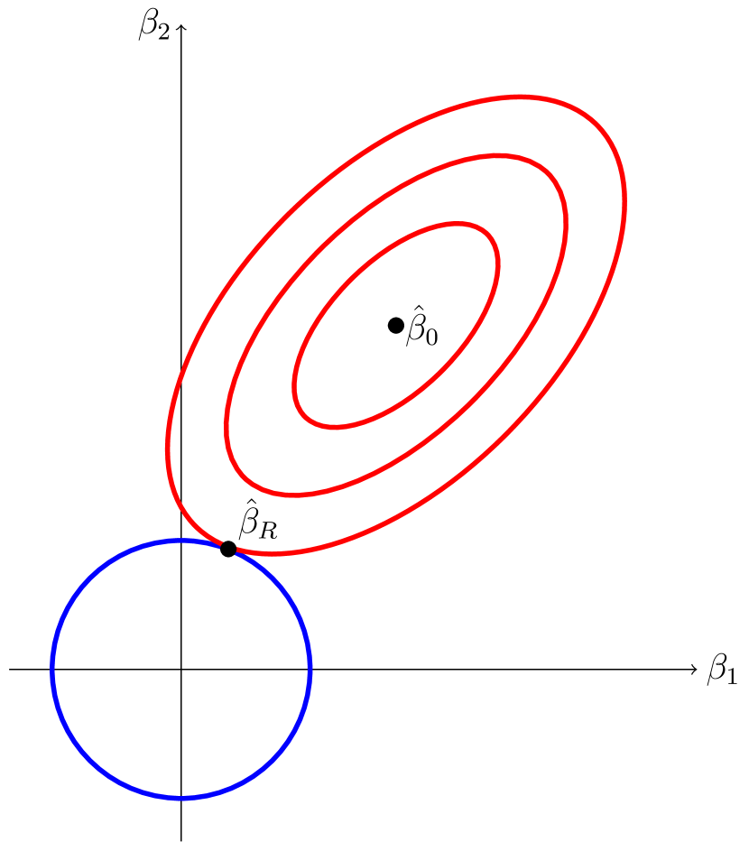
(a) Ridge

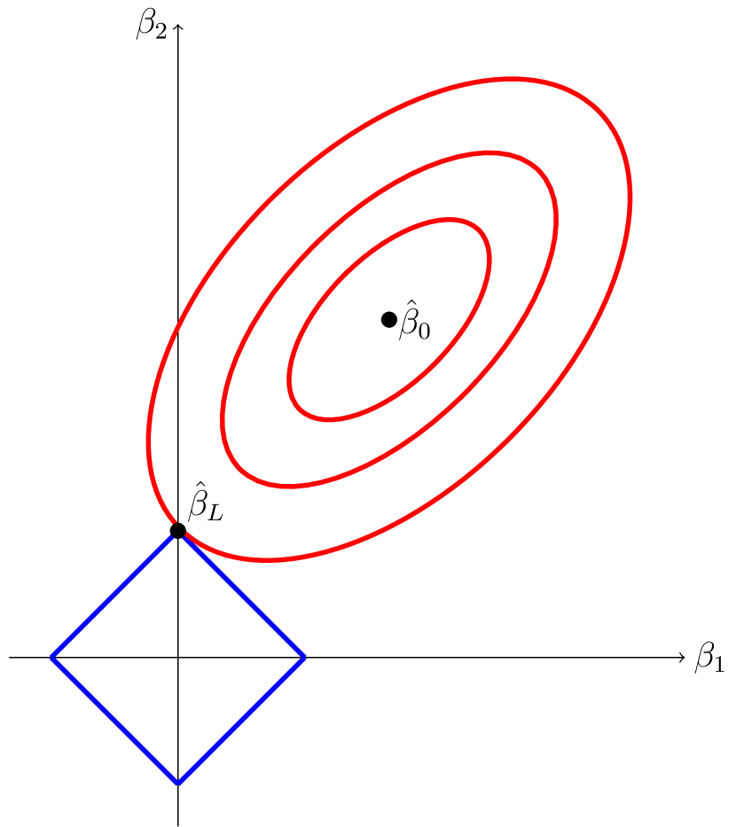
(b) Lasso

Figure 1: Behaviour of $\ell_{1}$ and $\ell_{2}$-penalty in comparison. Red lines represent RSS contour lines and the blue lines represent the lasso and ridge constraint, respectively. $\hat{\beta}_{0}$ denotes the OLS estimate. $\hat{\beta}_{L}$ and $\hat{\beta}_{R}$ are the lasso and ridge estimate. The illustration is based on Tibshirani, 1996, Fig. 2.

While there exists no closed form solution for the lasso, the ridge solution can be expressed as

$$\bm{\hat{\beta}}_{\textrm{ridge}}=(\bm{X}^{\prime}\bm{X}+\lambda\bm{\Psi}^{\prime}\bm{\Psi})^{-1}\bm{X}^{\prime}\bm{y}.$$

Here $\bm{X}$ is the $n\times p$ matrix of predictors with typical element $x_{ij}$, $\bm{y}$ is the response vector and $\bm{\Psi}=\textrm{diag}(\psi_{1},\ldots,\psi_{p})$ is the diagonal matrix of penalty loadings. The ridge regularizes the regressor matrix by adding positive constants to the diagonal of $\bm{X}^{\prime}\bm{X}$. The ridge solution is thus well-defined generally as long as all the $\psi_{j}$ and $\lambda$ are sufficiently large even if $\bm{X}^{\prime}\bm{X}$ is rank-deficient.

Elastic net

The elastic net of Zou and Hastie (2005) combines some of the strengths of lasso and ridge regression. It applies a mix of $\ell_{1}$ (lasso-type) and $\ell_{2}$ (ridge-type) penalization:

$$\bm{\hat{\beta}}_{\textrm{elastic}}=\arg\min\frac{1}{n}\sum_{i=1}^{n}\left(y_{i}-\bm{x}_{i}^{\prime}\bm{\beta}\right)^{2}+\frac{\lambda}{n}\left[\alpha\sum_{j=1}^{p}\psi_{j}|\beta_{j}|+(1-\alpha)\sum_{j=1}^{p}\psi_{j}^{2}\beta_{j}^{2}\right]$$ (3)

The additional parameter $\alpha$ determines the relative to contribution of $\ell_{1}$ vs. $\ell_{2}$ penalization. In the presence of groups of correlated regressors, the lasso typically selects only one variable from each group, whereas the ridge tends to produce similar coefficient estimates for groups of correlated variables. On the other hand, the ridge does not yield sparse solutions impeding model interpretation. The elastic net is able to produce sparse solutions for some $\alpha$ greater than zero, and retains or drops correlated variables jointly.

Adaptive lasso

The irrepresentable condition (IRC) is shown to be sufficient and (almost) necessary for the lasso to be model selection consistent (Zhao and Yu, 2006; Meinshausen and Bühlmann, 2006). However, the IRC imposes strict constraints on the degree of correlation between predictors in the true model and predictors outside of the model. Motivated by this non-trivial condition for the lasso to be variable selection consistent, Zou (2006) proposed the adaptive lasso. The adaptive lasso uses penalty loadings of $\psi_{j}=1/|\hat{\beta}_{0,j}|^{\theta}$ where $\hat{\beta}_{0,j}$ is an initial estimator. The adaptive lasso is variable-selection consistent for fixed $p$ under weaker assumptions than the standard lasso. If $p<n$, OLS can be used as the initial estimator. Huang et al. (2008) prove variable selection consistency for large $p$ and suggest using univariate OLS if $p>n$. The idea of adaptive penalty loadings can also be applied to elastic net and ridge regression (Zou and Zhang, 2009).

Square-root lasso

The square-root lasso,

$$\bm{\hat{\beta}}_{\sqrt{\textrm{lasso}}}=\arg\min\sqrt{\frac{1}{n}\sum_{i=1}^{n}\left(y_{i}-\bm{x}_{i}^{\prime}\bm{\beta}\right)^{2}}+\frac{\lambda}{n}\sum_{j=1}^{p}\psi_{j}|\beta_{j}|,$$ (4)

is a modification of the lasso that minimizes the root mean squared error, while also imposing an $\ell_{1}$-penalty. The main advantage of the square-root lasso over the standard lasso becomes apparent if theoretically grounded, data-driven penalization is used. Specifically, the score vector, and thus the optimal penalty level, is independent of the unknown error variance under homoskedasticity as shown by Belloni et al. (2011), resulting in a simpler procedure for choosing $\lambda$ (see Section 5).

Post-estimation OLS

Penalized regression methods induce an attenuation bias that can be alleviated by post-estimation OLS, which applies OLS to the variables selected by the first-stage variable selection method, i.e.,

$$\bm{\hat{\beta}}_{\textrm{post}}=\arg\min\frac{1}{n}\sum_{i=1}^{n}\left(y_{i}-\bm{x}_{i}^{\prime}\bm{\beta}\right)^{2}\qquad\textrm{subject to}\qquad\beta_{j}=0~{}~{}\textrm{if}~{}~{}\tilde{\beta}_{j}=0,$$ (5)

where $\tilde{\beta}_{j}$ is a sparse first-step estimator such as the lasso. Thus, post-estimation OLS treats the first-step estimator as a genuine model selection technique. For the case of the lasso, Belloni and Chernozhukov (2013) have shown that the post-estimation OLS, also referred to as post-lasso, performs at least as well as the lasso under mild additional assumptions if theory-driven penalization is employed. Similar results hold for the square-root lasso (Belloni et al., 2011, 2014b).

2.2 Choice of the tuning parameters

Since coefficient estimates and the set of selected variables depend on $\lambda$ and $\alpha$, a central question is how to choose these tuning parameters. Which method is most appropriate depends on the objectives and setting: in particular, the aim of the analysis (prediction or model identification), computational constraints, and if and how the i.i.d. assumption is violated. lassopack offers three approaches for selecting the penalty level of $\lambda$ and $\alpha$:

1. Information criteria: The value of $\lambda$ can be selected using information criteria. lasso2 implements model selection using four information criteria. We discuss this approach in Section 3.

2. Cross-validation: The aim of cross-validation is to optimize the out-of-sample prediction performance. Cross-validation is implemented in cvlasso, which allows for cross-validation across both $\lambda$ and the elastic net parameter $\alpha$. See Section 4.

3. Theory-driven (‘rigorous’): Theoretically justified and feasible penalty levels and loadings are available for the lasso and square-root lasso via rlasso. The penalization is chosen to dominate the noise of the data-generating process (represented by the score vector), which allows derivation of theoretical results with regard to consistent prediction and parameter estimation. See Section 5.

3 Tuning parameter selection using information criteria

Information criteria are closely related to regularization methods. The classical Akaike’s information criterion (Akaike, 1974, AIC) is defined as $-2\times\textnormal{log-likelihood}+2p$. Thus, the AIC can be interpreted as penalized likelihood which imposes a penalty on the number of predictors included in the model. This form of penalization, referred to as $\ell_{0}$-penalty, has, however, an important practical disadvantage. In order to find the model with the lowest AIC, we need to estimate all different model specifications. In practice, it is often not feasible to consider the full model space. For example, with only 20 predictors, there are more than 1 million different models.

The advantage of regularized regression is that it provides a data-driven method for reducing model selection to a one-dimensional problem (or two-dimensional problem in the case of the elastic net) where we need to select $\lambda$ (and $\alpha)$. Theoretical properties of information criteria are well-understood and they are easy to compute once coefficient estimates are obtained. Thus, it seems natural to utilize the strengths of information criteria as model selection procedures to select the penalization level.

Information criteria can be categorized based on two central properties: loss efficiency and model selection consistency. A model selection procedure is referred to as loss efficient if it yields the smallest averaged squared error attainable by all candidate models. Model selection consistency requires that the true model is selected with probability approaching 1 as $n\rightarrow\infty$. Accordingly, which information information criteria is appropriate in a given setting also depends on whether the aim of analysis is prediction or identification of the true model.

We first consider the most popular information criteria, AIC and Bayesian information criterion (Schwarz, 1978, BIC):

$$\mathrm{AIC}(\lambda,\alpha) =n\log\left(\hat{\sigma}^{2}(\lambda,\alpha)\right)+2{df}(\lambda,\alpha),$$

$$\mathrm{BIC}(\lambda,\alpha) =n\log\left(\hat{\sigma}^{2}(\lambda,\alpha)\right)+{{df}}(\lambda,\alpha)\log(n),$$

where $\hat{\sigma}^{2}(\lambda,\alpha)=n^{-1}\sum_{i=1}^{n}\hat{\varepsilon}_{i}^{2}$ and $\hat{\varepsilon}_{i}$ are the residuals. ${{df}}(\lambda,\alpha)$ is the effective degrees of freedom, which is a measure of model complexity. In the linear regression model, the degrees of freedom is simply the number of regressors. Zou et al. (2007) show that the number of coefficients estimated to be non-zero, $\hat{s}$, is an unbiased and consistent estimate of ${{df}}(\lambda)$ for the lasso ($\alpha=1$). More generally, the degrees of freedom of the elastic net can be calculated as the trace of the projection matrix, i.e.,

$$\widehat{{df}}(\lambda,\alpha)=\textrm{tr}(\bm{X}_{\hat{\Omega}}(\bm{X}_{\hat{\Omega}}^{\prime}\bm{X}_{\hat{\Omega}}+\lambda(1-\alpha)\bm{\Psi})^{-1}\bm{X}_{\hat{\Omega}}^{\prime}).$$

where $\bm{X}_{\hat{\Omega}}$ is the $n\times\hat{s}$ matrix of selected regressors. The unbiased estimator of the degrees of freedom provides a justification for using the classical AIC and BIC to select tuning parameters (Zou et al., 2007).

The BIC is known to be model selection consistent if the true model is among the candidate models, whereas AIC is inconsistent. Clearly, the assumption that the true model is among the candidates is strong; even the existence of the ‘true model’ may be problematic, so that loss efficiency may become a desirable second-best. The AIC is, in contrast to BIC, loss efficient. Yang (2005) shows that the differences between AIC-type information criteria and BIC are fundamental; a consistent model selection method, such as the BIC, cannot be loss efficient, and vice versa. Zhang et al. (2010) confirm this relation in the context of penalized regression.

Both AIC and BIC are not suitable in the large-$p$-small-$n$ context where they tend to select too many variables (see Monte Carlo simulations in Section 8). It is well known that the AIC is biased in small samples, which motivated the bias-corrected AIC (Sugiura, 1978; Hurvich and Tsai, 1989),

$$\mathrm{AIC}_{c}(\lambda,\alpha)=n\log\left(\hat{\sigma}^{2}(\lambda,\alpha)\right)+2{df}(\lambda,\alpha)\frac{n}{n-{df}(\lambda,\alpha)}.$$

The bias can be severe if $df$ is large relative to $n$, and thus the AIC_c should be favoured when $n$ is small or with high-dimensional data.

The BIC relies on the assumption that each model has the same prior probability. This assumptions seems reasonable when the researcher has no prior knowledge; yet, it contradicts the principle of parsimony and becomes problematic if $p$ is large. To see why, consider the case where $p=1000$ (following Chen and Chen, 2008): There are $1000$ models for which one parameter is non-zero ($s=1$), while there are $1000\times 999/2$ models for which $s=2$. Thus, the prior probability of $s=2$ is larger than the prior probability of $s=1$ by a factor of $999/2$. More generally, since the prior probability that $s=j$ is larger than the probability that $s=j-1$ (up to the point where $j=p/2$), the BIC is likely to over-select variables. To address this shortcoming, Chen and Chen (2008) introduce the Extended BIC, defined as

$$\mathrm{EBIC}_{\xi}(\lambda,\alpha)=n\log\left(\hat{\sigma}^{2}(\lambda,\alpha)\right)+{{df}}(\lambda,\alpha)\log(n)+2\xi{{df}}(\lambda,\alpha)\log(p),$$

which imposes an additional penalty on the size of the model. The prior distribution is chosen such that the probability of a model with dimension $j$ is inversely proportional to the total number of models for which $s=j$. The additional parameter, $\xi\in[0,1]$, controls the size of the additional penalty. Chen and Chen (2008) show in simulation studies that the EBIC_ξ outperforms the traditional BIC, which exhibits a higher false discovery rate when $p$ is large relative to $n$.

4 Tuning parameter selection using cross-validation

The aim of cross-validation is to directly assess the performance of a model on unseen data. To this end, the data is repeatedly divided into a training and a validation data set. The models are fit to the training data and the validation data is used to assess the predictive performance. In the context of regularized regression, cross-validation can be used to select the tuning parameters that yield the best performance, e.g., the best out-of-sample mean squared prediction error. A wide range of methods for cross-validation are available. For an extensive review, we recommend Arlot and Celisse (2010). The most popular method is $K$-fold cross-validation, which we introduce in Section 4.1. In Section 4.2, we discuss methods for cross-validation in the time-series setting.

4.1 K-fold cross-validation

For $K$-fold cross-validation, proposed by Geisser (1975), the data is split into $K$ groups, referred to as folds, of approximately equal size. Let $\mathcal{K}_{k}$ denote the set of observations in the $k$th fold, and let $n_{k}$ be the size of data partition $k$ for $k=1,...,K$. In the $k$th step, the $k$th fold is treated as the validation data set and the remaining $K-1$ folds constitute the training data set. The model is fit to the training data for a given value of $\lambda$ and $\alpha$. The resulting estimate, which is based on all the data except the observations in fold $k$, is $\bm{\hat{\beta}}_{k}(\lambda,\alpha)$. The procedure is repeated for each fold, as illustrated in Figure 2, so that every data point is used for validation once. The mean squared prediction error for each fold is computed as

$$\textrm{MSPE}_{k}(\lambda,\alpha)=\frac{1}{n_{k}}\sum_{i\in\mathcal{K}_{k}}\left(y_{i}-\bm{x}_{i}^{\prime}\bm{\hat{\beta}}_{k}(\lambda,\alpha)\right)^{2}.$$

Figure 2: Data partition for 5-fold cross-validation. Each row corresponds to one step and each column to one data partition (‘fold’). In the first step, fold 1 constitutes the validation data and folds 2-5 are the training data.

The $K$-fold cross-validation estimate of the MSPE, which serves as a measure of prediction performance, is

$$\hat{\mathcal{L}}^{CV}(\lambda,\alpha)=\frac{1}{K}\sum_{k=1}^{K}\textrm{MSPE}_{k}(\lambda,\alpha).$$

This suggests selecting $\lambda$ and $\alpha$ as the values that minimize $\hat{\mathcal{L}}^{CV}(\lambda,\alpha)$. An alternative common rule is to use the largest value of $\lambda$ that is within one standard deviation of the minimum, which leads to a more parsimonious model.

Cross-validation can be computationally expensive. It is necessary to compute $\hat{\mathcal{L}}^{CV}$ for each value of $\lambda$ on a grid if $\alpha$ is fixed (e.g. when using the lasso) or, in the case of the elastic net, for each combination of values of $\lambda$ and $\alpha$ on a two-dimensional grid. In addition, the model must be estimated $K$ times at each grid point, such that the computational cost is approximately proportional to $K$.

Standardization adds another layer of computational cost to $K$-fold cross validation. An important principle in cross-validation is that the training data set should not contain information from the validation dataset. This mimics the real-world situation where out-of-sample predictions are made not knowing what the true response is. The principle applies not only to individual observations, but also to data transformations such as mean-centering and standardization. Specifically, data transformations applied to the training data should not use information from the validation data or full dataset. Mean-centering and standardization using sample means and sample standard deviations for the full sample would violate this principle. Instead, when in each step the model is fit to the training data for a given $\lambda$ and $\alpha$, the training dataset must be re-centered and re-standardized, or, if standardization is built into the penalty loadings, the $\hat{\psi}_{j}$ must be recalculated based on the training dataset.

The choice of $K$ is not only a practical problem; it also has theoretical implications. The variance of $\hat{\mathcal{L}}^{CV}$ decreases with $K$, and is minimal (for linear regression) if $K=n$, which is referred to as leave-one-out or LOO CV. Similarly, the bias decreases with the size of the training data set. Given computational contraints, $K$ between 5 and 10 are often recommended, arguing that the performance of CV rarely improves for $K$ larger than 10 (Hastie et al., 2009; Arlot and Celisse, 2010).

If the aim of the researcher’s analysis is model identification rather than prediction, the theory requires training data to be ‘small’ and the evaluation sample to be close to $n$ (Shao, 1993, 1997). The reason is that more data is required to evaluate which model is the ‘correct’ one rather than to decrease bias and variance. This is referred to as cross-validation paradox (Yang, 2006). However, since $K$-fold cross-validation sets the size of the training sample to approximately $n/K$, $K$-fold CV is necessarily ill-suited for selecting the true model.

4.2 Cross-validation with time-series data

Serially dependent data violate the principle that training and validation data are independent. That said, standard $K$-fold cross-validation may still be appropriate in certain circumstances. Bergmeir et al. (2018) show that $K$-fold cross-validation remains valid in the pure auto-regressive model if one is willing to assume that the errors are uncorrelated. A useful implication is that $K$-fold cross-validation can be used on overfit auto-regressive models that are not otherwise badly misspecified, since such models have uncorrelated errors.

Rolling $h$-step ahead CV is an intuitively appealing approach that directly incorporates the ordered nature of time series-data (Hyndman, Rob and Athanasopoulos, 2018). The procedure builds on repeated $h$-step ahead forecasts. The procedure is implemented in lassopack and illustrated in Figure 3-4.

		Step
		1	2	3	4	5
	1	$T$	$T$	$T$	$T$	$T$ [t]
	2	$T$	$T$	$T$	$T$	$T$
	3	$T$	$T$	$T$	$T$	$T$
$t$	4	$V$	$T$	$T$	$T$	$T$
	5	$\cdot$	$V$	$T$	$T$	$T$
	6	$\cdot$	$\cdot$	$V$	$T$	$T$
	7	$\cdot$	$\cdot$	$\cdot$	$V$	$T$
	8	$\cdot$	$\cdot$	$\cdot$	$\cdot$	$V$

(a) $h=1$, expanding window

		Step
		1	2	3	4	5
	1	$T$	$T$	$T$	$T$	$T$ [t]
	2	$T$	$T$	$T$	$T$	$T$
	3	$T$	$T$	$T$	$T$	$T$
$t$	4	$\cdot$	$T$	$T$	$T$	$T$
	5	$V$	$\cdot$	$T$	$T$	$T$
	6	$\cdot$	$V$	$\cdot$	$T$	$T$
	7	$\cdot$	$\cdot$	$V$	$\cdot$	$T$
	8	$\cdot$	$\cdot$	$\cdot$	$V$	$\cdot$
	9	$\cdot$	$\cdot$	$\cdot$	$\cdot$	$V$

(b) $h=2$, expanding window

Figure 3: Rolling $h$-step ahead cross-validation with expanding training window. ‘$T$’ and ‘$V$’ denote that the observation is included in the training and validation sample, respectively. A dot (‘.’) indicates that an observation is excluded from both training and validation data.

		Step
		1	2	3	4	5
	1	$T$	$\cdot$	$\cdot$	$\cdot$	$\cdot$ [t]
	2	$T$	$T$	$\cdot$	$\cdot$	$\cdot$
	3	$T$	$T$	$T$	$\cdot$	$\cdot$
$t$	4	$V$	$T$	$T$	$T$	$\cdot$
	5	$\cdot$	$V$	$T$	$T$	$T$
	6	$\cdot$	$\cdot$	$V$	$T$	$T$
	7	$\cdot$	$\cdot$	$\cdot$	$V$	$T$
	8	$\cdot$	$\cdot$	$\cdot$	$\cdot$	$V$

(a) $h=1$, fixed window

		Step
		1	2	3	4	5
	1	$T$	$\cdot$	$\cdot$	$\cdot$	$\cdot$ [t]
	2	$T$	$T$	$\cdot$	$\cdot$	$\cdot$
	3	$T$	$T$	$T$	$\cdot$	$\cdot$
$t$	4	$\cdot$	$T$	$T$	$T$	$\cdot$
	5	$V$	$\cdot$	$T$	$T$	$T$
	6	$\cdot$	$V$	$\cdot$	$T$	$T$
	7	$\cdot$	$\cdot$	$V$	$\cdot$	$T$
	8	$\cdot$	$\cdot$	$\cdot$	$V$	$\cdot$
	9	$\cdot$	$\cdot$	$\cdot$	$\cdot$	$V$

(b) $h=2$, fixed window

Figure 4: Rolling $h$-step ahead cross-validation with fixed training window.

Figure 3(a) corresponds to the default case of 1-step ahead cross-validation. ‘$T$’ denotes the observation included in the training sample and ‘$V$’ refers to the validation sample. In the first step, observations 1 to 3 constitute the training data set and observation 4 is the validation point, whereas the remaining observations are unused as indicated by a dot (‘.’). Figure 3(b) illustrates the case of 2-step ahead cross-validation. In both cases, the training window expands incrementally, whereas Table 4 displays rolling CV with a fixed estimation window.

4.3 Comparison with information criteria

Since information-based approaches and cross-validation share the aim of model selection, one might expect that the two methods share some theoretical properties. Indeed, AIC and LOO-CV are asymptotically equivalent, as shown by Stone (1977) for fixed $p$. Since information criteria only require the model to be estimated once, they are computationally much more attractive, which might suggest that information criteria are superior in practice. However, an advantage of CV is its flexibility and that it adapts better to situations where the assumptions underlying information criteria, e.g. homoskedasticity, are not satisfied (Arlot and Celisse, 2010). If the aim of the analysis is identifying the true model, BIC and EBIC provide a better choice than $K$-fold cross-validation, as there are strong but well-understood conditions under which BIC and EBIC are model selection consistent.

5 Rigorous penalization

This section introduces the ‘rigorous’ approach to penalization. Following Chernozhukov et al. (2016), we use the term ‘rigorous’ to emphasize that the framework is grounded in theory. In particular, the penalization parameters are chosen to guarantee consistent prediction and parameter estimation. Rigorous penalization is of special interest, as it provides the basis for methods to facilitate causal inference in the presence of many instruments and/or many control variables; these methods are the IV-Lasso (Belloni et al., 2012), the post-double-selection (PDS) estimator (Belloni et al., 2014a) and the post-regularization estimator (CHS) (Chernozhukov et al., 2015); all of which are implemented in our sister package pdslasso (Ahrens et al., 2018).

We discuss the conditions required to derive theoretical results for the lasso in Section 5.1. Sections 5.2-5.5 present feasible algorithms for optimal penalization choices for the lasso and square-root lasso under i.i.d., heteroskedastic and cluster-dependent errors. Section 5.6 presents a related test for joint significance testing.

5.1 Theory of the lasso

There are three main conditions required to guarantee that the lasso is consistent in terms of prediction and parameter estimation. The first condition relates to sparsity. Sparsity is an attractive assumption in settings where we have a large set of potentially relevant regressors, or consider various different model specifications, but assume that only one true model exists which includes a small number of regressors. We have introduced exact sparsity in Section 2, but the assumption is stronger than needed. For example, some true coefficients may be non-zero, but small in absolute size, in which case it might be preferable to omit them. For this reason, we use a weaker assumption:

Approximate sparsity.

Belloni et al. (2012) consider the approximate sparse model (ASM),

$$y_{i}=f(\bm{w}_{i})+\varepsilon_{i}=\bm{x}_{i}^{\prime}\bm{\beta}_{0}+r_{i}+\varepsilon_{i}.$$ (6)

The elementary regressors $\bm{w}_{i}$ are linked to the dependent variable through the unknown and possibly non-linear function $f(\cdot)$. The aim of the lasso (and square-root lasso) estimation is to approximate $f(\bm{w}_{i})$ using the target parameter vector $\bm{\beta}_{0}$ and the transformations $\bm{x}_{i}:=P(\bm{w}_{i})$, where $P(\cdot)$ denotes a dictionary of transformations. The vector $\bm{x}_{i}$ may be large relative to the sample size, either because $\bm{w}_{i}$ itself is high-dimensional and $\bm{x}_{i}:=\bm{w}_{i}$, or because a large number of transformations such as dummies, polynomials, interactions are considered to approximate $f(\bm{w}_{i})$.

The assumption of approximate sparsity requires the existence of a target vector $\bm{\beta}_{0}$ which ensures that $f(\bm{w}_{i})$ can be approximated sufficiently well, while using only a small number of non-zero coefficients. Specifically, the target vector $\bm{\beta}_{0}$ and the sparsity index $s$ are assumed to meet the condition

$$\lVert\bm{\beta}_{0}\rVert_{0}:=s\ll n\qquad\mathrm{with}\quad\frac{s^{2}\log^{2}(p\vee n)}{n}\rightarrow 0,$$

and the resulting approximation error $r_{i}=f(\bm{w}_{i})-\bm{x}_{i}^{\prime}\bm{\beta}_{0}$ is bounded such that

$$\sqrt{\frac{1}{n}\sum_{i=1}^{n}r_{i}^{2}}\leq C\sqrt{\frac{s}{n}},$$ (7)

where $C$ is a positive constant. To emphasize the distinction between approximate and exact sparsity, consider the special case where $f(\bm{w}_{i})$ is linear with $f(\bm{w}_{i})=\bm{x}_{i}^{\prime}\bm{\beta}^{\star}$, but where the true parameter vector $\bm{\beta}^{\star}$ violates exact sparsity so that $\lVert\bm{\beta}^{\star}\rVert_{0}>n$. If $\bm{\beta}^{\star}$ has many elements that are negligible in absolute size, we might still be able to approximate $\bm{\beta}^{\star}$ using the sparse target vector $\bm{\beta}_{0}$ as long as $r_{i}=\bm{x}_{i}^{\prime}(\bm{\beta}^{\star}-\bm{\beta}_{0})$ is sufficiently small as specified in (7).

Restricted sparse eigenvalue condition.

The second condition relates to the Gram matrix, $n^{-1}\bm{X}^{\prime}\bm{X}$. In the high-dimensional setting where $p$ is larger than $n$, the Gram matrix is necessarily rank-deficient and the minimum (unrestricted) eigenvalue is zero, i.e.,

$$\min_{\bm{\delta}\neq 0}\frac{\left\lVert\bm{X}\bm{\delta}\right\rVert_{2}}{\sqrt{n}\left\lVert\bm{\delta}\right\rVert_{2}}=0.$$

Thus, to accommodate large $p$, the full rank condition of OLS needs to be replaced by a weaker condition. While the full rank condition cannot hold for the full Gram matrix if $p>n$, we can plausibly assume that sub-matrices of size $m$ are well-behaved. This is in fact the restricted sparse eigenvalue (RSEC) condition of Belloni et al. (2012). The RSEC formally states that the minimum sparse eigenvalues

$$\phi_{\min}(m)=\min_{1\leq\lVert\bm{\delta}\rVert_{0}\leq m}\frac{\bm{\delta}^{\prime}\bm{X}^{\prime}\bm{X}\bm{\delta}}{\lVert\bm{\delta}\rVert^{2}_{2}}\qquad\mathrm{and}\qquad\phi_{\max}(m)=\max_{1\leq\lVert\bm{\delta}\rVert_{0}\leq m}\frac{\bm{\delta}^{\prime}\bm{X}^{\prime}\bm{X}\bm{\delta}}{\lVert\bm{\delta}\rVert^{2}_{2}}$$

are bounded away from zero and from above. The requirement $\phi_{\min}(m)>0$ implies that all sub-matrices of size $m$ have to be positive definite.

Regularization event.

The third central condition concerns the choice of the penalty level $\lambda$ and the predictor-specific penalty loadings $\psi_{j}$. The idea is to select the penalty parameters to control the random part of the problem in the sense that

$$\frac{\lambda}{n}\geq c\max_{1\leq j\leq p}\big{|}\psi_{j}^{-1}S_{j}\big{|}\quad\textnormal{where}\quad S_{j}=\frac{2}{n}\sum_{i=1}^{n}x_{ij}\varepsilon_{i}$$ (8)

with high probability. Here, $c>1$ is a constant slack parameter and $S_{j}$ is the $j$th element of the score vector $\bm{S}=\nabla\hat{Q}(\bm{\beta})$, the gradient of $\hat{Q}$ at the true value $\bm{\beta}$. The score vector summarizes the noise associated with the estimation problem.

Denote by $\Lambda=n\max_{j}|\psi_{j}^{-1}S_{j}|$ the maximal element of the score vector scaled by $n$ and $\psi_{j}$, and denote by $q_{\Lambda}(\cdot)$ the quantile function for $\Lambda$. In the rigorous lasso, we choose the penalty parameters $\lambda$ and $\psi_{j}$ and confidence level $\gamma$ so that

$$\lambda\geq cq_{\Lambda}(1-\gamma)$$ (9)

A simple example illustrates the intuition behind this approach. Consider the case where the true model has $\beta_{j}=0$ for $j=1,\ldots,p$, i.e., none of the regressors appear in the true model. It can be shown that for the lasso to select no variables, the penalty parameters $\lambda$ and $\psi_{j}$ need to satisfy $\lambda\geq 2\max_{j}|\sum_{i}\psi_{j}^{-1}x_{ij}y_{i}|$. Because none of the regressors appear in the true model, $y_{i}=\varepsilon_{i}$. We can therefore rewrite the requirement for the lasso to correctly identify the model without regressors as $\lambda\geq 2\max_{j}|\sum_{i}\psi_{j}^{-1}x_{ij}\varepsilon_{i}|$, which is the regularization event in (8). We want this regularization event to occur with high probability of at least $(1-\gamma)$. If we choose values for $\lambda$ and $\psi_{j}$ such that $\lambda\geq q_{\Lambda}(1-\gamma)$, then by the definition of a quantile function we will choose the correct model—no regressors—with probability of at least $(1-\gamma)$. This is simply the rule in (9).

The chief practical problem in using the rigorous lasso is that the quantile function $q_{\Lambda}(\cdot)$ is unknown. There are two approaches to addressing this problem proposed in the literature, both of which are implemented in rlasso. The rlasso default is the ‘asymptotic’ or X-independent approach: theoretically grounded and feasible penalty level and loadings are used that guarantee that (8) holds asymptotically, as $n\rightarrow\infty$ and $\gamma\rightarrow 0$. The X-independent penalty level choice can be interpreted as an asymptotic upper bound on the quantile function $q_{\Lambda}(.)$. In the ‘exact’ or X-dependent approach, the quantile function $q_{\Lambda}(.)$ is directly estimated by simulating the distribution of $q_{\Lambda}(1-\gamma|\bm{X})$, the $(1-\gamma)$-quantile of $\Lambda$ conditional on the observed regressors $\bm{X}$. We first focus on the X-independent approach, and introduce the X-dependent approach in Section 5.5.

5.2 Rigorous lasso

Belloni et al. (2012) show—using moderate deviation theory of self-normalized sums from Jing et al. (2003)—that the regularization event in (8) holds asymptotically, i.e.,

$$\mathrm{P}\left(\max_{1\leq j\leq p}c\,\big{|}S_{j}\big{|}\leq\frac{\lambda\psi_{j}}{n}\right)\rightarrow 1~{}~{}\textrm{as}~{}~{}n\rightarrow\infty,~{}\gamma\rightarrow 0.$$ (10)

if the penalty levels and loadings are set to

$$\begin{array}[]{lll}\textrm{homoskedasticity:}&\lambda=2c\sigma\sqrt{n}\Phi^{-1}(1-\gamma/(2p)),&\quad\psi_{j}=\sqrt{\dfrac{1}{n}\sum_{i}x_{ij}^{2}},\\ \textrm{heteroskedasticity:}&\lambda=2c\sqrt{n}\Phi^{-1}(1-\gamma/(2p)),&\quad\psi_{j}=\sqrt{\dfrac{1}{n}\sum_{i}x_{ij}^{2}\varepsilon_{i}^{2}},\end{array}$$ (11)

under homoskedasticity and heteroskedasticity, respectively. $c$ is the slack parameter from above and the significance level $\gamma$ is required to converge towards 0. rlasso uses $c=1.1$ and $\gamma=0.1/\log(n)$ as defaults.^,

Homoskedasticity.

We first focus on the case of homoskedasticity. In the rigorous lasso approach, we standardize the score. But since $E(x_{ij}^{2}\varepsilon_{i}^{2})=\sigma E(x_{ij}^{2})$ under homoskedasticity, we can separate the problem into two parts: the regressor-specific penalty loadings $\psi_{j}=\sqrt{(1/n)\sum_{i}x_{ij}^{2}}$ standardize the regressors, and $\sigma$ moves into the overall penalty level. In the special case where the regressors have already been standardized such that $(1/n)\sum_{i}x_{ij}^{2}=1$, the penalty loadings are $\psi_{j}=1$. Hence, the purpose of the regressor-specific penalty loadings in the case of homoskedasticity is to accommodate regressors with unequal variance.

The only unobserved term is $\sigma$, which appears in the optimal penalty level $\lambda$. To estimate $\sigma$, we can use some initial set of residuals $\hat{\varepsilon}_{0,i}$ and calculate the initial estimate as $\hat{\sigma}_{0}=\sqrt{(1/n)\sum_{i}\hat{\varepsilon}_{0,i}^{2}}$. A possible choice for the initial residuals is $\hat{\varepsilon}_{0,i}=y_{i}$ as in Belloni et al. (2012) and Belloni et al. (2014a). rlasso uses the OLS residuals $\hat{\varepsilon}_{0,i}=y_{i}-\bm{x}_{i}[\mathcal{D}]^{\prime}\hat{\bm{\beta}}_{OLS}$ where $\mathcal{D}$ is the set of 5 regressors exhibiting the highest absolute correlation with $y_{i}$. The procedure is summarized in Algorithm A:

= 2pt = 1pt = .2pt  Algorithm A: Estimation of penalty level under homoskedasticity.

1. Set $k=0$, and define the maximum number of iterations, $K$. Regress $y_{i}$ against the subset of $d$ predictors exhibiting the highest correlation coefficient with $y_{i}$ and compute the initial residuals as $\hat{\varepsilon}_{0,i}=\hat{\varepsilon}_{k,i}=y_{i}-\bm{x}_{i}[\mathcal{D}]^{\prime}\hat{\bm{\beta}}_{OLS}$. Calculate the homoskedastic penalty loadings in (11).

2. If $k\leq K$, compute the homoskedastic penalty level in (11) by replacing $\sigma$ with $\hat{\sigma}_{k}=\sqrt{(1/n)\sum_{i}\hat{\varepsilon}_{k,i}^{2}},$ and obtain the rigorous lasso or post-lasso estimator $\hat{\bm{\beta}}_{k}$. Update the residuals $\hat{\varepsilon}_{k+1,i}=y_{i}-\bm{x}_{i}^{\prime}\hat{\bm{\beta}}_{k}$. Set $k\leftarrow k+1$.

3. Repeat step 2 until $k>K$ or until convergence by updating the penalty level.

= 2pt = 1pt = .2pt

The rlasso default is to perform one further iteration after the initial estimate (i.e., $K=1$), which in our experience provides good performance. Both lasso and post-lasso can be used to update the residuals. rlasso uses post-lasso to update the residuals.

Heteroskedasticity.

The X-independent choice for the overall penalty level under heteroskedasticity is $\lambda=2c\sqrt{n}\Phi^{-1}(1-\gamma/(2p))$. The only difference with the homoskedastic case is the absence of $\varsigma$. The variance of $\epsilon$ is now captured via the penalty loadings, which are set to $\psi_{j}=\sqrt{\frac{1}{n}\sum_{i}x_{ij}^{2}\varepsilon_{i}^{2}}$. Hence, the penalty loadings here serve two purposes: accommodating both heteroskedasticity and regressors with uneven variance.

To help with the intuition, we consider the case where the predictors are already standardized. It is easy to see that, if the errors are homoskedastic with $\sigma=1$, the penalty loadings are (asymptotically) just $\psi_{j}=1$. If the data are heteroskedastic, however, the standardized penalty loading will not be $1$. In most practical settings, the usual pattern will be that $\hat{\psi}_{j}>1$ for some $j$. Intuitively, heteroskedasticity typically increases the likelihood that the term $\max_{j}|\sum_{i}x_{ij}\varepsilon_{i}|$ takes on extreme values, thus requiring a higher degree of penalization through the penalty loadings.

The disturbances $\varepsilon_{i}$ are unobserved, so we obtain an initial set of penalty loadings $\hat{\psi}_{j}$ from an initial set of residuals $\hat{\varepsilon}_{0,i}$ similar to the i.i.d. case above. We summarize the algorithm for estimating the penalty level and loadings as follows:

= 2pt = 1pt = .2pt  Algorithm B: Estimation of penalty loadings under heteroskedasticity.

1. Set $k=0$, and define the maximum number of iterations, $K$. Regress $y_{i}$ against the subset of $d$ predictors exhibiting the highest correlation coefficient with $y_{i}$ and compute the initial residuals as $\hat{\varepsilon}_{0,i}=\hat{\varepsilon}_{k,i}=y_{i}-\bm{x}_{i}[\mathcal{D}]^{\prime}\hat{\bm{\beta}}_{OLS}$. Calculate the heteroskedastic penalty level $\lambda$ in (11).

2. If $k\leq K$, compute the heterokedastic penalty loadings using the formula given in in (11) by replacing $\varepsilon_{i}$ with $\hat{\varepsilon}_{k,i}$, obtain the rigorous lasso or post-lasso estimator $\hat{\bm{\beta}}_{k}$. Update the residuals $\hat{\varepsilon}_{k+1,i}=y_{i}-\bm{x}_{i}^{\prime}\hat{\bm{\beta}}_{k}$. Set $k\leftarrow k+1$.

3. Repeat step 2 until $k>K$ or until convergence by updating the penalty loadings.

= 2pt = 1pt = .2pt

Theoretical property.

Under the assumptions SEC, ASM and if penalty level $\lambda$ and the penalty loadings are estimated by Algorithm A or B, the lasso and post-lasso obey:

$$\sqrt{\frac{1}{n}\sum_{i=1}^{n}\left(\bm{x_{i}}^{\prime}\bm{\hat{\beta}}-\bm{x_{i}}^{\prime}\bm{\beta}\right)^{2}} =O\left(\sqrt{\frac{s\log(p\vee n)}{n}}\right),$$ (12)

$$\lVert\bm{\hat{\beta}}-\bm{\beta}\rVert_{1} =O\left(\sqrt{\frac{s^{2}\log(p\vee n)}{n}}\right),$$ (13)

The first relation in (12) provides an asymptotic bound for the prediction error, and the second relation in (13) bounds the bias in estimating the target parameter $\bm{\beta}$. Belloni et al. (2012) refer to the above convergence rates as near-oracle rates. If the identity of the $s$ variables in the model were known, the prediction error would converge at the oracle rate $\sqrt{s/n}$. Thus, the logarithmic term $\log(p\vee n)$ can be interpreted as the cost of not knowing the true model.

5.3 Rigorous square-root lasso

The theory of the square-root lasso is similar to the theory of the lasso (Belloni et al., 2011, 2014b). The $j$th element of the score vector is now defined as

$$S_{j}=\frac{\frac{1}{n}\sum_{i=1}^{n}x_{ij}\varepsilon_{i}}{\left\{\frac{1}{n}\sum_{i=1}^{n}\varepsilon_{i}^{2}\right\}^{1/2}}.$$ (14)

To see why the square-root lasso is of special interest, we define the standardized errors $\nu_{i}$ as $\nu_{i}=\varepsilon_{i}/\sigma$. The $j$th element of the score vector becomes

$$S_{j}=\frac{\frac{1}{n}\sum_{i=1}^{n}x_{ij}\sigma\nu_{i}}{\left\{\frac{1}{n}\sum_{i=1}^{n}\sigma^{2}\nu_{i}^{2}\right\}^{1/2}}=\frac{\frac{1}{n}\sum_{i=1}^{n}x_{ij}\nu_{i}}{\left\{\frac{1}{n}\sum_{i=1}^{n}\nu_{i}^{2}\right\}^{1/2}}$$ (15)

and is thus independent of $\sigma$. For the same reason, the optimal penalty level for the square-root lasso in the i.i.d. case,

$$\lambda=c\sqrt{n}\Phi^{-1}(1-\gamma/(2p)),$$ (16)

is independent of the noise level $\sigma$.

Homoskedasticity.

The ideal penalty loadings under homoskedasticity for the square-root lasso are given by formula (iv) in Table 1, which provides an overview of penalty loading choices. The ideal penalty parameters are independent of the unobserved error, which is an appealing theoretical property and implies a practical advantage. Since both $\lambda$ and $\psi_{j}$ can be calculated from the data, the rigorous square-root lasso is a one-step estimator under homoskedasticity. Belloni et al. (2011) show that the square-root lasso performs similarly to the lasso with infeasible ideal penalty loadings.

Heteroskedasticity.

In the case of heteroskedasticity, the optimal square-root lasso penalty level remains (16), but the penalty loadings, given by formula (v) in Table 1, depend on the unobserved error and need to be estimated. Note that the updated penalty loadings using the residuals $\hat{\varepsilon}_{i}$ employ thresholding: the penalty loadings are enforced to be greater than or equal to the loadings in the homoskedastic case. The rlasso default algorithm used to obtain the penalty loadings in the heteroskedastic case is analogous to Algorithm B. While the ideal penalty loadings are not independent of the error term if the errors are heteroskedastic, the square-root lasso may still have an advantage over the lasso, since the ideal penalty loadings are pivotal with respect to the error term up to scale, as pointed out above.

5.4 Rigorous penalization with panel data

Belloni et al. (2016) extend the rigorous framework to the case of clustered data, where a limited form of dependence—within-group correlation—as well as heteroskedasticity are accommodated. They prove consistency of the rigorous lasso using this approach in the large $n$, fixed $T$ and large $n$, large $T$ settings. The authors present the approach in the context of a fixed-effects panel data model, $y_{it}=\bm{x}_{it}^{\prime}\bm{\beta}+\mu_{i}+\varepsilon_{it}$, and apply the rigorous lasso after the within transformation to remove the fixed effects $\mu_{i}$. The approach extends to any clustered-type setting and to balanced and unbalanced panels. For convenience we ignore the fixed effects and write the model as a balanced panel:

$$y_{it}=\bm{x}_{it}^{\prime}\bm{\beta}+\varepsilon_{it}\quad\quad i=1,\ldots,n,~{}t=1,\ldots,T$$ (17)

The intuition behind the Belloni et al. (2016) approach is similar to that behind the clustered standard errors reported by various Stata estimation commands: observations within clusters are aggregated to create ‘super-observations’ which are assumed independent, and these super-observations are treated similarly to cross-sectional observations in the non-clustered case. Specifically, define for the $i$th cluster and $j$th regressor the super-observation $u_{ij}:=\sum_{t}x_{ijt}\varepsilon_{it}$. Then the penalty loadings for the clustered case are

$$\psi_{j}=\sqrt{\frac{1}{nT}\sum_{i=1}^{n}u_{ij}^{2}},$$

which resembles the heteroskedastic case. The rlasso default for the overall penalty level is the same as in the heteroskedastic case, $\lambda=2c\sqrt{n}\Phi^{-1}(1-\gamma/(2p))$, except that the default value for $\gamma$ is $0.1/\log(n)$, i.e., we use the number of clusters $n$ rather than the number of observations $nT$. lassopack also implements the rigorous square-root lasso for panel data, which uses the overall penalty in (16) and the penalty loadings in formula (vi), Table 1.

	lasso		square-root lasso
homoskedasticity	(i)	$\displaystyle\sqrt{\frac{1}{n}\sum_{i=1}^{n}x_{ij}^{2}}$	(iv)	$\displaystyle\sqrt{\frac{1}{n}\sum_{i=1}^{n}x_{ij}^{2}}$
heteroskedasticity	(ii)	$\displaystyle\sqrt{\frac{1}{n}\sum_{i=1}^{n}x_{ij}^{2}\varepsilon_{i}^{2}}$	(v)	$\displaystyle\sqrt{\frac{1}{n}\sum_{i=1}^{n}x_{ij}^{2}}~{}\vee~{}\sqrt{\frac{\sum_{i=1}^{n}x_{ij}^{2}\varepsilon_{i}^{2}}{\sum_{i=1}^{n}\varepsilon_{i}^{2}}}$
cluster-dependence	(iii)	$\displaystyle\sqrt{\frac{1}{nT}\sum_{i=1}^{n}u_{ij}^{2}}$	(vi)	$\displaystyle\sqrt{\frac{1}{nT}\sum_{i=1}^{n}\sum_{t}^{T}x_{ijt}^{2}}~{}\vee~{}\sqrt{\frac{\sum_{i=1}^{n}u_{ij}^{2}}{\sum_{i=1}^{n}\sum_{t=1}^{T}\varepsilon_{it}^{2}}}$
Note: Formulas (iii) and (vi) use the notation $u_{ij}=\sum_{t}x_{itj}\varepsilon_{it}$.

Table 1: Ideal penalty loadings for the lasso and square-root lasso under homoskedasticity, heteroskedasticity and cluster-dependence.

5.5 X-dependent lambda

There is an alternative, sharper choice for the overall penalty level, referred to as the X-dependent penalty. Recall that the asymptotic, X-independent choice in (11) can be interpreted as an asymptotic upper bound on the quantile function of $\Lambda$, which is the scaled maximum value of the score vector. Instead of using the asymptotic choice, we can estimate by simulation the distribution of $\Lambda$ conditional on the observed $\bm{X}$, and use this simulated distribution to obtain the quantile $q_{\Lambda}(1-\gamma|\bm{X})$.

	lasso		square-root lasso
homoskedasticity	(i)	$\displaystyle 2\hat{\sigma}\max_{1\leq j\leq p}\left|\sum_{i=1}^{n}\psi_{j}^{-1}x_{ij}g_{i}\right|$	(iv)	$\displaystyle\frac{1}{\hat{\sigma}_{g}}\max_{1\leq j\leq p}\left|\sum_{i=1}^{n}\psi_{j}^{-1}x_{ij}g_{i}\right|$
heteroskedasticity	(ii)	$\displaystyle 2\max_{1\leq j\leq p}\left|\sum_{i=1}^{n}\psi_{j}^{-1}x_{ij}\hat{\varepsilon}_{i}g_{i}\right|$	(v)	$\displaystyle\frac{1}{\hat{\sigma}_{g}}\max_{1\leq j\leq p}\left|\sum_{i=1}^{n}\psi_{j}^{-1}x_{ij}\hat{\varepsilon}_{i}g_{i}\right|$
cluster-dependence	(iii)	$\displaystyle 2\max_{1\leq j\leq p}\left|\sum_{i=1}^{n}\psi_{j}^{-1}\hat{u}_{ij}g_{i}\right|$	(vi)	$\displaystyle\frac{1}{\hat{\sigma}_{g}}\max_{1\leq j\leq p}\left|\sum_{i=1}^{n}\psi_{j}^{-1}\hat{u}_{ij}g_{i}\right|$
Note: $g_{i}$ is an i.i.d. standard normal variate drawn independently of the data; $\hat{\sigma}_{g}=\frac{1}{n}\sum_{i}g_{i}^{2}$. Formulas (iii) and (vi) use the notation $\hat{u}_{ij}=\sum_{t}x_{itj}\hat{\varepsilon}_{it}$.

Table 2: Definition of $W$ statistic for the simulation of the distribution of $\Lambda$ for the lasso and square-root lasso under homoskedasticity, heteroskedasticity and cluster-dependence.

In the case of estimation by the lasso under homoskedasticity, we simulate the distribution of $\Lambda$ using the statistic $W$, defined as

$$W=2\hat{\sigma}\max_{1\leq j\leq p}\left|\sum_{i=1}^{n}\psi_{j}^{-1}x_{ij}g_{i}\right|,$$

where $\psi_{j}$ is the penalty loading for the homoskedastic case, $\hat{\sigma}$ is an estimate of the error variance using some previously-obtained residuals, and $g_{i}$ is an i.i.d. standard normal variate drawn independently of the data. The X-dependent penalty choice is sharper and adapts to correlation in the regressor matrix (Belloni and Chernozhukov, 2011).

Under heteroskedasticity, the lasso X-dependent penalty is obtained by a multiplier bootstrap procedure. In this case the simulated statistic $W$ is defined as in formula (ii) in Table 2. The cluster-robust X-dependent penalty is again obtained analogously to the heteroskedastic case by defining super-observations, and the statistic $W$ is defined as in formula (iii) in Table 2. Note that the standard normal variate $g_{i}$ varies across but not within clusters.

The X-dependent penalties for the square-root lasso are similarly obtained from quantiles of the simulated distribution of the square-root lasso $\Lambda$, and are given by formulas (iv), (v) and (vi) in Table 2 for the homoskedastic, heteroskedastic and clustered cases, respectively.

5.6 Significance testing with the rigorous lasso

Inference using the lasso, especially in the high-dimensional setting, is a challenging and ongoing research area of research (see Footnote 2). A test that has been developed and is available in rlasso corresponds to the test for joint significance of regressors using $F$ or $\chi^{2}$ tests that is common in regression analysis. Specifically, Belloni et al. (2012) suggest using the Chernozhukov et al. (2013, Appendix M) sup-score test to test for the joint significance of the regressors, i.e.,

$$H_{0}:\beta_{1}=\ldots=\beta_{p}=0.$$

As in the preceding sections, regressors are assumed to be mean-centered and in their original units.

If the null hypothesis is correct and the rest of the model is well-specified, including the assumption that the regressors are orthogonal to the disturbance $\varepsilon_{i}$, then $y_{i}=\varepsilon_{i}$ and hence $E(\bm{x}_{i}\varepsilon_{i})=E(\bm{x}_{i}y_{i})=0$. The sup-score statistic is

$$S_{SS}=\sqrt{n}\max_{1\leq j\leq p}\left|\frac{1}{n}\sum_{i=1}^{n}\psi_{j}^{-1}x_{ij}y_{i}\right|$$ (18)

where $\psi_{j}=\sqrt{\frac{1}{n}\sum_{i=1}^{n}(x_{ij}y_{i})^{2}}$. Intuitively, the $\psi_{j}$ in (18) plays the same role as the penalty loadings do in rigorous lasso estimation.

The $p$-value for the sup-score test is obtained by a multiplier bootstrap procedure simulating the distribution of $S_{SS}$ by the statistic $W$, defined as

$$W=\sqrt{n}\max_{1\leq j\leq p}\left|\frac{1}{n}\sum_{i=1}^{n}\psi_{j}^{-1}x_{ij}y_{i}g_{i}\right|,$$

where $g_{i}$ is an i.i.d. standard normal variate drawn independently of the data and $\psi_{j}$ is defined as in (18).

The procedure above is valid under both homoskedasticity and heteroskedasticity, but requires independence. A cluster-robust version of the sup-score test that accommodates within-group dependence is

$$S_{SS}=\sqrt{nT}\max_{1\leq j\leq p}\Big{|}\frac{1}{nT}\sum_{i=1}^{n}\psi_{j}^{-1}u_{ij}\Big{|}$$ (19)

where $u_{ij}:=\sum_{t=1}^{T}x_{ijt}y_{it}$ and $\psi_{j}=\frac{1}{nT}\sum_{i=1}^{n}u_{ij}^{2}$.

The $p$-value for the cluster version of $S_{SS}$ comes from simulating

$$W=\sqrt{nT}\max_{1\leq j\leq p}\Big{|}\frac{1}{nT}\sum_{i=1}^{n}\psi_{j}^{-1}u_{ij}g_{i}\Big{|}$$

where again $g_{i}$ is an i.i.d. standard normal variate drawn independently of the data. Note again that $g_{i}$ is invariant within clusters.

rlasso also reports conservative critical values for $S_{SS}$ using an asymptotically-justified upper bound: $CV=c\Phi^{-1}(1-\gamma_{SS}/(2p))$. The default value of the slack parameter is $c=1.1$ and the default test level is $\gamma_{SS}=0.05$. These parameters can be varied using the c(real) and ssgamma(real) options, respectively. The simulation procedure to obtain $p$-values using the simulated statistic $W$ can be computationally intensive, so users can request reporting of only the computationally inexpensive conservative critical values by setting the number of simulated values to zero with the ssnumsim(int) option.

6 The commands

The package lassopack consists of three commands: lasso2, cvlasso and rlasso. Each command offers an alternative method for selecting the tuning parameters $\lambda$ and $\alpha$. We discuss each command in turn and present its syntax. We focus on the main syntax and the most important options. Some technical options are omitted for the sake of brevity. For a full description of syntax and options, we refer to the help files.

6.1 lasso2: Base command and information criteria

The primary purpose of lasso2 is to obtain the solution of (adaptive) lasso, elastic net and square-root lasso for a single value of $\lambda$ or a list of penalty levels, i.e., for $\lambda_{1},\ldots,\lambda_{r},\ldots,\lambda_{R}$, where $R$ is the number of penalty levels. The basic syntax of lasso2 is as follows:

lasso2 depvar indepvars $\bigl{[}$ if $\bigr{]}$ $\bigl{[}$ in $\bigr{]}$ $\bigl{[}$ , alpha() sqrt adaptive adaloadings(numlist) adatheta(real) ols lambda(numlist) lcount(integer) lminratio() lmax() notpen(varlist) partial(varlist) ploadings(string) unitloadings prestd stdcoef fe noconstant tolopt() tolzero() maxiter(integer) plotpath(method) plotvar(varlist) plotopt(string) plotlabel lic(string) ic(string) ebicxi() postresults $\bigr{]}$

The options alpha(real), sqrt, adaptive and ols can be used to select elastic net, square-root lasso, adaptive lasso and post-estimation OLS, respectively. The default estimator of lasso2 is the lasso, which corresponds to alpha(1). The special case of alpha(0) yields ridge regression.

The behaviour of lasso2 depends on whether the numlist in lambda(numlist) is of length greater than one or not. If numlist is a list of more than one value, the solution consists of a matrix of coefficient estimates which are stored in e(betas). Each row in e(betas) corresponds to a distinct value of $\lambda_{r}$ and each column to one of the predictors in indepvars. The ‘path’ of coefficient estimates over $\lambda_{r}$ can be plotted using plotpath(method), where method controls whether the coefficient estimates are plotted against lambda (‘lambda’), the natural logarithm of lambda (‘lnlambda’) or the $\ell_{1}$-norm (‘norm’). If the numlist in lambda(numlist) is a scalar value, the solution is a vector of coefficient estimates which is stored in e(b). The default behaviour of lasso2 is to use a list of 100 values.

In addition to obtaining the coefficient path, lasso2 calculates four information criteria (AIC, AIC_c, BIC and EBIC). These information criteria can be used for model selection by choosing the value of $\lambda_{r}$ that yields the lowest value for one of the four information criteria. The ic(string) option controls which information criterion is shown in the output, where string can be replaced with ‘aic’, ‘aicc’, ‘bic or ‘ebic’. lic(string) displays the estimation results corresponding to the model selected by an information criterion. It is important to note that lic(string) will not store the results of the estimation. This has the advantage that the user can compare the results for different information criteria without the need to re-estimate the full model. To save the estimation results, the postresults option should be specified in combination with lic(string).

Estimation methods

alpha(real) controls the elastic net parameter, $\alpha$, which controls the degree of $\ell_{1}$-norm (lasso-type) to $\ell_{2}$-norm (ridge-type) penalization. alpha(1) corresponds to the lasso (the default estimator), and alpha(0) to ridge regression. The real value must be in the interval [0,1].

sqrt specifies the square-root lasso estimator. Since the square-root lasso does not employ any form of $\ell_{2}$-penalization, the option is incompatible with alpha(real).

adaptive specifies the adaptive lasso estimator. The penalty loading for predictor $j$ is set to $|\hat{\beta}_{j,0}|^{-\theta}$ where $\hat{\beta}_{j,0}$ is the OLS estimator or univariate OLS estimator if $p>n$. $\theta$ is the adaptive exponent, and can be controlled using the adatheta(real) option.

adaloadings(matrix)  is a matrix of alternative initial estimates, $\hat{\beta}_{j,0}$, used for calculating adaptive loadings. For example, this could be the vector e(b) from an initial lasso2 estimation. The absolute value of $\hat{\beta}_{j,0}$ is raised to the power $-\theta$ (note the minus).

adatheta(real)  is the exponent for calculating adaptive penalty loadings. The default is adatheta(1)

ols specifies that post-estimation OLS estimates are displayed and returned in e(betas) or e(b).

Options relating to lambda

lambda(numlist) controls the penalty level(s), $\lambda_{r}$, used for estimation. numlist is a scalar value or list of values in descending order. Each $\lambda_{r}$ must be greater than zero. If not specified, the default list is used which, using Mata syntax, is defined by

exp(rangen(log(lmax),log(lminratio*lmax),lcount)),

where lcount, lminratio and lmax are defined below, exp() is the exponential function, log() is the natural logarithm, and rangen(a,b,n) creates a column vector going from a to b in n-1 steps (see the mf_range help file). Thus, the default list ranges from lmax to lminratio*lmax and lcount is the number of values. The distance between each $\lambda_{r}$ in the sequence is the same on the logarithmic scale.

lcount(integer) is the number of penalty values, $R$, for which the solution is obtained. The default is lcount(100).

lmax() is the maximum value penalty level, $\lambda_{1}$. By default, $\lambda_{1}$ is chosen as the smallest penalty level for which the model is empty. Suppose the regressors are mean-centered and standardized, then $\lambda_{1}$ is defined as $\max_{j}\frac{2}{n\alpha}\sum_{i=1}^{n}|x_{ij}y_{i}|$ for the elastic net and $\max_{j}\frac{1}{n\alpha}\sum_{i=1}^{n}|x_{ij}y_{i}|$ for the square-root lasso (see Friedman et al., 2010, Section 2.5).

lminratio() is the ratio of the minimum penalty level, $\lambda_{R}$, to maximum penalty level, $\lambda_{1}$.  must be between 0 and 1. Default is lminratio(0.001).

Information criteria

lic(string) specifies that, after the first lasso2 estimation using a list of penalty levels, the model that corresponds to the minimum information criterion will be estimated and displayer. ‘aic’, ‘bic’, ‘aicc’, and ‘ebic’ (the default) are allowed. However, the results are not stored in e().

postresults is used in combination with lic(string). postresults stores estimation results of the model selected by information criterion in e().

ic(string) controls which information criterion is shown in the output of lasso2 when lambda() is a list. ’aic’, ’bic’, ’aicc’, and ’ebic’ (the default are allowed).

ebicxi() controls the $\xi$ parameter of the EBIC. $\xi$ needs to lie in the [0,1] interval. $\xi=0$ is equivalent to the BIC. The default choice is $\xi=1-\log(n)/(2\log(p))$.

Penalty loadings and standardisation

notpen(varlist) sets penalty loadings to zero for predictors in varlist. Unpenalized predictors are always included in the model.

partial(varlist) specified that variables in varlist are partialled out prior to estimation.

ploadings(matrix) is a row-vector of penalty loadings, and overrides the default standardization loadings. The size of the vector should equal the number of predictors (excluding partialled-out variables and excluding the constant).

unitloadings specifies that penalty loadings be set to a vector of ones; overrides the default standardization loadings.

prestd specifies that dependent variable and predictors are standardized prior to estimation rather than standardized “on the fly” using penalty loadings. See Section 9.2 for more details. By default the coefficient estimates are un-standardized (i.e., returned in original units).

stdcoef returns coefficients in standard deviation units, i.e., do not un-standardize. Only supported with prestd option.

Penalty loadings and standardisation

fe within-transformation is applied prior to estimation. The option requires the data in memory to be xtset.

noconstant suppress constant from estimation. Default behaviour is to partial the constant out (i.e., to center the regressors).

Replay syntax

The replay syntax of lasso2 allows for plotting and changing display options, without the need to re-run the full model. It can also be used to estimate the model using the value of $\lambda$ selected by an information criterion. The syntax is given by:

lasso2 $\bigl{[}$ , plotpath(string) plotvar(varlist) plotopt(string) plotlabel postresults lic(method) ic(method) $\bigr{]}$

Prediction syntax

predict $\bigl{[}\,$type$\,\bigr{]}$ newvar $\bigl{[}$ if $\bigr{]}$ $\bigl{[}$ in $\bigr{]}$ $\bigl{[}$ , xb residuals ols lambda() lid(integer) approx noisily postresults $\bigr{]}$

xb computes predicted values (the default).

residuals computes residuals.

ols specifies that post-estimation OLS will be used for prediction.

If the previous lasso2 estimation uses more than one penalty level (i.e. $R>1$), the following options are applicable:

lambda() specifies that lambda value used for prediction.

lid(integer) specifies the index of the lambda value used for prediction.

approx specifies that linear approximation is used instead of re-estimation. Faster, but only exact if coefficient path is piece-wise linear.

noisily prompts display of estimation output if re-estimation required.

postresults stores estimation results in e() if re-estimation is used.

6.2 Cross-validation with cvlasso

cvlasso implements $K$-fold and $h$-step ahead rolling cross-validation. The syntax of cvlasso is:

cvlasso depvar indepvars $\bigl{[}$ if $\bigr{]}$ $\bigl{[}$ in $\bigr{]}$ $\bigl{[}$ , alpha(numlist) alphacount(integer) sqrt adaptive adaloadings(string) adatheta() ols lambda(numlist) lcount(stinteger) lminratio() lmax() lopt lse notpen(varlist) partial(varlist) ploadings(string) unitloadings prestd fe noconstant tolopt() tolzero() maxiter(integer) nfolds(integer) foldvar(varname) savefoldvar(varname) rolling h(integer) origin(integer) fixedwindow seed(integer) plotcv plotopt(string) saveest(string) $\bigr{]}$

The alpha() option of cvlasso option accepts a numlist, while lasso2 only accepts a scalar. If the numlist is a list longer than one, cvlasso cross-validates over $\lambda_{r}$ with $r=1,\ldots,R$ and $\alpha_{m}$ with $m=1,\ldots,M$.

plotcv creates a plot of the estimated mean-squared prediction error as a function of $\lambda_{r}$, and plotopt(string) can be used to pass plotting options to Stata’s line command.

Internally, cvlasso calls lasso2 repeatedly. Intermediate lasso2 results can be stored using saveest(string).

Options for K-fold cross-validation

nfolds(integer) is the number of folds used for $K$-fold cross-validation. The default is nfolds(10), or $K=10$.

foldvar(varname) can be used to specify what fold (data partition) each observation lies in. varname is an integer variable with values ranging from 1 to $K$. If not specified, the fold variable is randomly generated such that each fold is of approximately equal size.

savefoldvar(varname) saves the fold variable variable in varname.

seed(integer) sets the seed for the generation of a random fold variable.

Options for h-step ahead rolling cross-validation

rolling uses rolling $h$-step ahead cross-validation. The option requires the data to be tsset or xtset.

h(integer) changes the forecasting horizon. The default is h(1).

origin(integer) controls the number of observations in the first training dataset.

fixedwindow ensures that the size of the training data set is constant.

Options for selection of lambda

lopt specifies that, after cross-validation, lasso2 estimates the model with the value of $\lambda_{r}$ that minimizes the mean-squared prediction error. That is, the model is estimated with $\lambda=\hat{\lambda}_{\texttt{lopt}}$.

lse specifies that, after cross-validation, lasso2 estimates model with largest $\lambda_{r}$ that is within one standard deviation from $\hat{\lambda}_{\texttt{lopt}}$. That is, the model is estimated with $\lambda=\hat{\lambda}_{\texttt{lse}}$.

postresults stores the lasso2 estimation results in e() (to be used in combination with lse or lopt).

Replay syntax

Similar to lasso2, cvlasso also provides a replay syntax, which helps to avoid time-consuming re-estimations. The replay syntax of cvlasso can be used for plotting and to estimate the model corresponding to $\hat{\lambda}_{\texttt{lopt}}$ or $\hat{\lambda}_{\texttt{lse}}$. The replay syntax of cvlasso is given by:

cvlasso $\bigl{[}$ , lopt lse plotcv(method) plotopt(string) postresults $\bigr{]}$

Predict syntax

predict $\bigl{[}\,$type$\,\bigr{]}$ newvar $\bigl{[}$ if $\bigr{]}$ $\bigl{[}$ in $\bigr{]}$ $\bigl{[}$ , xb residuals lopt lse noisily $\bigr{]}$

6.3 rlasso: Rigorous penalization

rlasso implements theory-driven penalization for lasso and square-root lasso. It allows for heteroskedastic, cluster-dependent and non-Gaussian errors. Unlike lasso2 and cvlasso, rlasso estimates the penalty level $\lambda$ using iterative algorithms. The syntax of rlasso is given by:

rlasso depvar indepvars $\bigl{[}$ if $\bigr{]}$ $\bigl{[}$ in $\bigr{]}$ $\bigl{[}$ weight $\bigr{]}$ $\bigl{[}$ , sqrt partial(varlist) pnotpen(varlist) noconstant fe robust cluster(variable) center xdependent numsim(integer) prestd tolopt() tolups() tolzero() maxiter(integer) maxpsiiter(integer) lassopsi corrnumber(integer) maxabsx lalternative gamma() c() supscore ssnumsim(integer) ssgamma() testonly seed(integer) ols  $\bigr{]}$

pnotpen(varlist) specifies that variables in varlist are not penalized.

robust specifies that the penalty loadings account for heteroskedasticity.

cluster(varname) specifies that the penalty loadings account for clustering on variable varname.

center center moments in heteroskedastic and cluster-robust loadings.

lassopsi use lasso or square-root lasso residuals to obtain penalty loadings. The default is post-estimation OLS.

corrnumber(integer) number of high-correlation regressors used to obtain initial residuals. The default is corrnumber(5), and corrnumber(0) implies that depvar is used in place of residuals.

prestd standardize data prior to estimation. The default is standardization during estimation via penalty loadings.

Options relating to lambda

xdependent specifies that the X-dependent penalty level is used; see Section 5.5.

numsim(integer) is the number of simulations used for the X-dependent case. The default is 5,000.

lalternative specifies the alternative, less sharp penalty level, which is defined as $2c\sqrt{2n\log(2p/\gamma)}$ (for the square-root lasso, $2c$ is replaced with $c$). See Footnote 12.

gamma() is the ‘$\gamma$’ in the rigorous penalty level (default ${\gamma}=1/{\log(n)}$; cluster-lasso default ${\gamma}=1/{\log(n_{clust})}$). See Equation (11).

c() is the ‘$c$’ in the rigorous penalty level. The default is c(1.1). See Equation (11).

Sup-score test

supscore reports the sup-score test of statistical significance.

testonly reports only the sup-score test without lasso estimation.

ssgamma() is the test level for the conservative critical value for the sup-score test (default = 0.05, i.e., 5% significance level).

ssnumsim(integer) controls the number of simulations for sup-score test multiplier bootstrap. The default is 500, while 0 implies no simulation.

Predict syntax

predict $\bigl{[}\,$type$\,\bigr{]}$ newvar $\bigl{[}$ if $\bigr{]}$ $\bigl{[}$ in $\bigr{]}$ $\bigl{[}$ , xb residuals lasso ols $\bigr{]}$

xb generate fitted values (default).

residuals generate residuals.

lasso use lasso coefficients for prediction (default is to use estimates posted in e(b) matrix).

ols use OLS coefficients based on lasso-selected variables for prediction (default is to use estimates posted in e(b) matrix).

7 Demonstrations

In this section, we demonstrate the use of lasso2, cvlasso and rlasso using one cross-section example (in Section 7.1) and one time-series example (in Section 7.2).

7.1 Cross-section

For demonstration purposes, we consider the Boston Housing Dataset available on the UCI Machine Learning Repository. The data set includes 506 observations and 14 predictors. The purpose of the analysis is to predict house prices using a set of census-level characteristics.

Estimation with lasso2

We first employ the lasso estimator:

• 
  

  . lasso2 medv crim-lstat
  
    Knot   ID     Lambda    s      L1-Norm        EBIC     R-sq     Entered/removed
                                                                                     
       1    1 6858.98553     1     0.00000   2250.74087   0.0000    Added _cons.
       2    2 6249.65216     2     0.08440   2207.91748   0.0924    Added lstat.
       3    3 5694.45029     3     0.28098   2166.62026   0.1737    Added rm.
       4   10 2969.09110     4     2.90443   1902.66627   0.5156    Added ptratio.
       5   20 1171.07071     5     4.79923   1738.09475   0.6544    Added b.
       6   22  972.24348     6     5.15524   1727.95402   0.6654    Added chas.
       7   26  670.12972     7     6.46233   1709.14648   0.6815    Added crim.
       8   28  556.35346     8     6.94988   1705.73465   0.6875    Added dis.
       9   30  461.89442     9     8.10548   1698.65787   0.6956    Added nox.
      10   34  318.36591    10    13.72934   1679.28783   0.7106    Added zn.
      11   39  199.94307    12    18.33494   1671.61672   0.7219    Added indus rad.
      12   41  165.99625    13    20.10743   1669.76857   0.7263    Added tax.
      13   47   94.98916    12    23.30144   1645.44345   0.7359    Removed indus.
      14   67   14.77724    13    26.71618   1642.91756   0.7405    Added indus.
      15   82    3.66043    14    27.44510   1648.83626   0.7406    Added age.
  Use ´long´ option for full output.
  Type e.g. ´lasso2, lic(ebic)´ to run the model selected by EBIC.
  

The above lasso2 output shows the following columns:

• Knot is the knot index. Knots are points at which predictors enter or leave the model. The default output shows one line per knot. If the long option is specified, one row per $\lambda_{r}$ value is shown.

• ID shows the $\lambda_{r}$ index, i.e., $r$. By default, lasso2 uses a descending sequence of 100 penalty levels.

• s is the number of predictors in the model.

• L1-Norm shows the $\ell_{1}$-norm of coefficient estimates.

• The sixth column (here labelled EBIC) shows one out of four information criteria. The ic(string) option controls which information criterion is displayed, where string can be replaced with ‘aic’, ‘aicc’, ‘bic’, and ‘ebic’ (the default).

• R-sq shows the $R^{2}$ value.

• The final column shows which predictors are entered or removed from the model at each knot. The order in which predictors are entered into the model can be interpreted as an indication of the relative predictive power of each predictor.

Since lambda() is not specified, lasso2 obtains the coefficient path for a default list of $\lambda_{r}$ values. The largest penalty level is 6858.99, in which case the model does only include the constant. Figure 5 shows the coefficient path of the lasso for selected variables as a function of $\ln(\lambda)$.

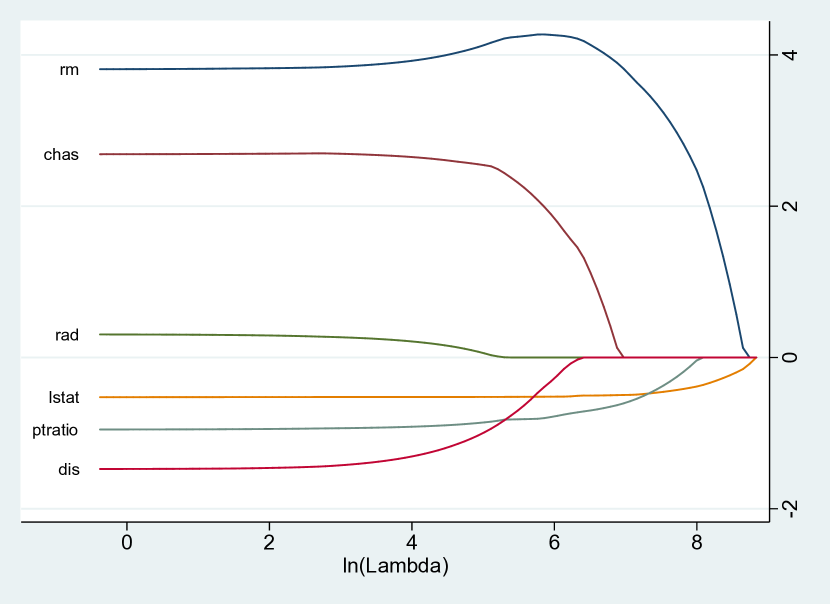
(a) Coefficient path

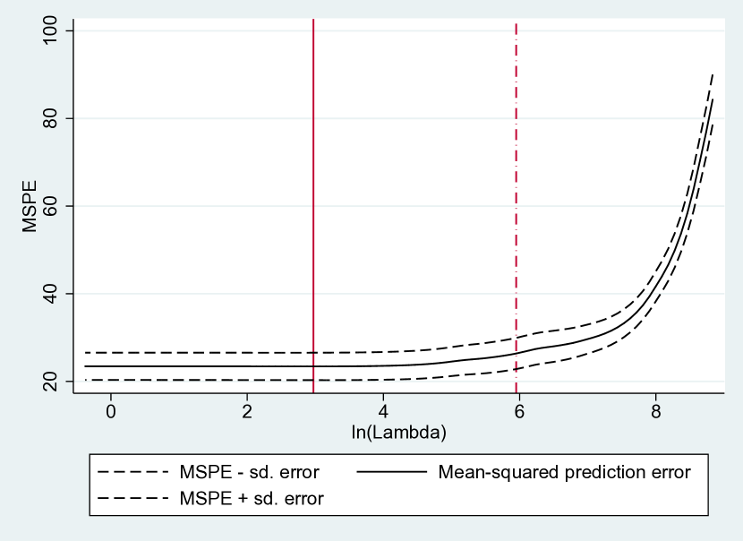
(b) Mean squared prediction error

Figure 5: The left graph shows the coefficient path of the lasso for selected variables as a function of $\ln(\lambda)$. The right graph shows the mean squared prediction error estimated by cross-validation along with $\pm$ one standard error. The continuous and dashed vertical lines correspond to lopt and lse, respectively.

lasso2 supports model selection using information criteria. To this end, we use the replay syntax in combination with the lic() option, which avoids that the full model needs to be estimated again. The lic() option can also be specified in the first lasso2 call. In the following example, the replay syntax works similar to a post-estimation command.

• 
  

  . lasso2, lic(ebic)
  
  Use lambda=16.21799867742649 (selected by EBIC).
  
                                                      
           Selected             Lasso   Post-est OLS
                                                      
               crim        -0.1028391     -0.1084133
                 zn         0.0433716      0.0458449
               chas         2.6983218      2.7187164
                nox       -16.7712529    -17.3760262
                 rm         3.8375779      3.8015786
                dis        -1.4380341     -1.4927114
                rad         0.2736598      0.2996085
                tax        -0.0106973     -0.0117780
            ptratio        -0.9373015     -0.9465246
                  b         0.0091412      0.0092908
              lstat        -0.5225124     -0.5225535
                                                      
     Partialled-out* 
                                                      
              _cons        35.2705812     36.3411478
                                                      
  

Two columns are shown in the output; one for the lasso estimator and one for post-estimation OLS, which applies OLS to the model selected by the lasso.

K-fold cross-validation with cvlasso

Next, we consider $K$-fold cross-validation.

• 
  

  . set seed 123
  
  . cvlasso medv crim-lstat
  
  K-fold cross-validation with 10 folds. Elastic net with alpha=1.
  Fold 1 2 3 4 5 6 7 8 9 10
                      Lambda           MSPE       st. dev.
                                                           
           1       6858.9855      84.302552      5.7124688
           2       6249.6522      77.022038      5.5626292
           3       5694.4503      70.352232      5.3037622
     (Output omitted.)
          30       461.89442      27.034557      3.5821586
          31       420.86099      26.695961      3.5812873
          32       383.47286      26.365176      3.5552884  ^
          33       349.40619      26.095202      3.5350981
          34       318.36591      25.857426        3.51782
     (Output omitted.)
          62       23.529539      23.421433      3.1339813
          63        21.43924      23.419627       3.131822
          64       19.534637      23.418936      3.1298343  *
          65       17.799234      23.419177      3.1280902
          66       16.217999      23.419668      3.1266572
     (Output omitted.)
          98       .82616724      23.441147      3.1134727
          99       .75277282      23.441321      3.1134124
         100       .68589855      23.441481      3.1133575
  * lopt = the lambda that minimizes MSPE.
    Run model: cvlasso, lopt
  ^ lse = largest lambda for which MSPE is within one standard error of the minimal MSPE.
    Run model: cvlasso, lse
  

The cvlasso output displays four columns: the index of $\lambda_{r}$ (i.e., $r$), the value of $\lambda_{r}$, the estimated mean squared prediction error, and the standard deviation of the mean squared prediction error. The output indicates the value of $\lambda_{r}$ that corresponds to the lowest MSPE with an asterisk (*). We refer to this value as $\hat{\lambda}_{\texttt{lopt}}$. In addition, the symbol ^ marks the largest value of $\lambda$ that is within one standard error of $\hat{\lambda}_{\texttt{lopt}}$, which we denote as $\hat{\lambda}_{\texttt{lse}}$.

The mean squared prediction is shown in Figure 5, which was created using the plotcv option. The graph shows the mean squared prediction error estimated by cross-validation along with $\pm$ one standard error. The continuous and dashed vertical lines correspond to $\hat{\lambda}_{\texttt{lopt}}$ and $\hat{\lambda}_{\texttt{lse}}$, respectively.

To estimate the model corresponding to either $\hat{\lambda}_{\texttt{lopt}}$ or $\hat{\lambda}_{\texttt{lse}}$, we use the lopt or lse option, respectively. Similar to the lic() option of lasso2, lopt and lse can either specified in the first cvlasso call or after estimation using the replay syntax as in this example:

• 
  

  . cvlasso, lopt
  Estimate lasso with lambda=19.535 (lopt).
  
                                                      
           Selected             Lasso   Post-est OLS
                                                      
               crim        -0.1016991     -0.1084133
                 zn         0.0428658      0.0458449
               chas         2.6941511      2.7187164
                nox       -16.6475746    -17.3760262
                 rm         3.8449399      3.8015786
                dis        -1.4268524     -1.4927114
                rad         0.2683532      0.2996085
                tax        -0.0104763     -0.0117780
            ptratio        -0.9354154     -0.9465246
                  b         0.0091106      0.0092908
              lstat        -0.5225040     -0.5225535
                                                      
     Partialled-out* 
                                                      
              _cons        35.0516465     36.3411478
                                                      
  

Rigorous penalization with rlasso

Lastly, we consider rlasso. The program rlasso runs an iterative algorithm to estimate the penalty level and loadings. In contrast to lasso2 and cvlasso, it reports the selected model directly.

• 
  

  . rlasso medv crim-lstat, supscore
  
                                                      
           Selected             Lasso   Post-est OLS
                                                      
               chas         0.6614716      3.3200252
                 rm         4.0224498      4.6522735
            ptratio        -0.6685443     -0.8582707
                  b         0.0036058      0.0101119
              lstat        -0.5009804     -0.5180622
              _cons  *     14.5986089     11.8535884
                                                      
  *Not penalized
  
  Sup-score test H0: beta=0
  CCK sup-score statistic  16.59 p-value= 0.000
  CCK 5% critical value     3.18 (asympt bound)
  

The supscore option prompts the sup-score test of joint significance. The $p$-value is obtained through multiplier bootstrap. The test statistic of 16.59 can also be compared to the asymptotic 5% critical value (here 3.18).

7.2 Time-series data

A standard problem in time-series econometrics is to select an appropriate lag length. In this sub-section, we show how lassopack can be employed for this purpose. We consider Stata’s built-in data set lutkepohl2.dta, which includes quarterly (log-differenced) consumption (dln_consump), investment (dln_inv) and income (dln_inc) series for West Germany over the period 1960, Quarter 1 to 1982, Quarter 4. We demonstrate both lag selection via information criteria and by $h$-step ahead rolling cross-validation. We do not consider the rigorous penalization approach of rlasso due to the assumption of independence, which seems too restrictive in the time-series context.

Information criteria

After importing the data, we run the most general model with up to 12 lags of dln_consump, dln_inv and dln_inc using lasso2 with lic(aicc) option.

• 
  

  . lasso2 dln_consump L(1/12).(dln_inv dln_inc dln_consump), lic(aicc) long
  
    Knot   ID     Lambda    s      L1-Norm        AICc     R-sq     Entered/removed
                                                                                     
       1    1    0.52531     1     0.00000   -714.43561   0.0000    Added _cons.
     (Output omitted.)
           11    0.20719    10     0.67593   -722.62355*  0.3078   
     (Output omitted.)
          100    0.00005    37     4.92856   -665.31816   0.6719   
  *indicates minimum AICc.
  Use lambda=.2071920751852477 (selected by AICC).
  
                                                      
           Selected             Lasso   Post-est OLS
                                                      
            dln_inv  
                L2.         0.0279780      0.0513004
                     
            dln_inc  
                L1.         0.0672531      0.1522251
                L2.         0.1184912      0.1675746
                L3.         0.0779780      0.1261940
                L8.        -0.1091959     -0.2481821
                     
        dln_consump  
                L2.         0.0259311      0.0935048
                L3.         0.0765755      0.1405377
               L10.         0.0833425      0.2320500
               L11.        -0.0891871     -0.1442602
                                                      
     Partialled-out* 
                                                      
                     
              _cons         0.0133270      0.0079518
                                                      
  

The output consists of two parts. The second part of the output is prompted since lic(aicc) is specified. lic(aicc) asks lasso2 to estimate the model selected by AIC_c, which in this case corresponds to $\lambda_{11}=0.207$.

h-step ahead rolling cross-validation

In the next step, we consider $h$-step ahead rolling cross-validation.

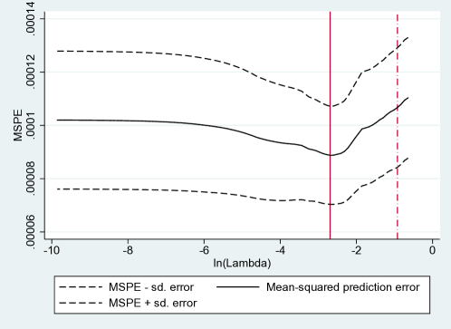
Figure 6: Cross-validation plot. The graph uses Stata’s built-in data set lutkepohl2.dta and 1-step ahead rolling cross-validation with origin(50).

• 
  

  . cvlasso dln_consump L(1/12).(dln_inv dln_inc dln_consump), rolling
  Rolling forecasting cross-validation with 1-step ahead forecasts. Elastic net with alpha=1.
  Training from-to (validation point): 13-80 (81), 13-81 (82), 13-82 (83), 13-83 (84),
  13-84 (85), 13-85 (86), 13-86 (87), 13-87 (88), 13-88 (89), 13-89 (> 90), 13-90 (91).
  

The output indicates how the data set is partitioned into training data and the validation point. For example, the short-hand 13-80 (81) in the output above indicates that observations 13 to 80 constitute the training data set in the first step of cross-validation, and observation 81 is the validation point. The options fixedwindow, h(integer) and origin(integer) can be used to control the partitioning of data into training and validation data. h(integer) sets the parameter $h$. For example, h(2) prompts 2-step ahead forecasts (the default is h(1)). fixedwindow ensures that the training data set is of same size in each step. If origin(50) is specified, the first training partition includes observations 13 to 50, as shown in the next example:

• 
  

  . cvlasso dln_consump L(1/12).(dln_inv dln_inc dln_consump), rolling origin(50) plotcv
  Rolling forecasting cross-validation with 1-step ahead forecasts. Elastic net with alpha=1.
  Training from-to (validation point): 13-50 (51), 13-51 (52), 13-52 (53), 13-53 (54),
     (Output omitted.)
  13-82 (83), 13-83 (84), 13-84 (85), 13-85 (86), 13-86 (87), 13-87 (88), 13-88 (89),
  13-89 (90), 13-90 (91).
  

The option plotcv creates the graph of the estimated mean squared prediction in Figure 6. To estimate the model corresponding to $\hat{\lambda}_{\texttt{lse}}$, we can as in the previous examples use the replay syntax:

• 
  

  . cvlasso, lse
  Estimate lasso with lambda=.397 (lse).
  
                                                      
           Selected             Lasso   Post-est OLS
                                                      
            dln_inv  
                L2.         0.0071068      0.0481328
                     
            dln_inc  
                L2.         0.0558422      0.2083321
                L3.         0.0253076      0.1479925
                     
        dln_consump  
                L3.         0.0260573      0.1079076
               L11.        -0.0299307     -0.1957719
                                                      
     Partialled-out* 
                                                      
                     
              _cons         0.0168736      0.0126810
                                                      
  

We point out that care should be taken when setting the parameters of $h$-step ahead rolling cross-validation. The default settings have no particular econometric justification.

8 Monte Carlo Simulation

We have introduced three alternative approaches for setting the penalization parameters in Sections 3-5. In this section, we present results of Monte Carlo simulations which assess the performance of these approaches in terms of in-sample fit, out-of-sample prediction, model selection and sparsity. To this end, we generate artificial data using the process

$$y_{i}=1+\sum_{j=1}^{p}\beta_{j}x_{ij}+\varepsilon_{i},\quad\varepsilon_{i}\sim\mathcal{N}(0,\sigma^{2}),\quad i=1,\ldots,2n,$$ (20)

with $n=200$. We report results for $p=100$ and for the high-dimensional setting with $p=220$. The predictors $x_{ij}$ are drawn from a multivariate normal distribution with $\textnormal{corr}(x_{ij},x_{ir})=0.9^{|j-r|}$. We vary the noise level $\sigma$ between $0.5$ and $5$; specifically, we consider $\sigma=\{0.5,1,2,3,5\}$. We define the parameters as $\beta_{j}=\mathbbm{1}\{j\leq s\}$ for $j=1,\ldots,p$ with $s=20$, implying exact sparsity. This simple design allows us to gain insights into the model selection performance in terms of false positive (the number of variables falsely included) and false negative frequency (the number of variables falsely omitted) when relevant and irrelevant regressors are correlated. All simulations use at least 1,000 iterations. We report additional Monte Carlo results in Appendix K, where we employ a design in which coefficients alternate in sign.

Since the aim is to assess in-sample and out-of-sample performance, we generate $2n$ observations, and use the data $i=1,\ldots,n$ as the estimation sample and the observations $i=n+1,\ldots,2n$ for assessing out-of-sample prediction performance. This allows us to calculate the root mean squared error (RMSE) and root mean squared prediction error (RMSPE) as

$$\textnormal{RMSE}=\sqrt{\frac{1}{n}\sum^{n}_{i=1}(y_{i}-\hat{y}_{i,n})^{2}}\qquad\textnormal{and}\qquad\textnormal{RMSPE}=\sqrt{\frac{1}{n}\sum^{2n}_{i=n+1}(y_{i}-\hat{y}_{i,n})^{2}},$$ (21)

where $\hat{y}_{i,n}$ are the predictions from fitting the model to the first $n$ observations.

Table 8 and 8 report results for the following estimation methods implemented in lassopack: the lasso with $\lambda$ selected by AIC, BIC, EBIC_ξ and AIC_c (as implemented in lasso2); the rigorous lasso and rigorous square-root lasso (implemented in rlasso), both using the X-independent and X-dependent penalty choice; and lasso with 5-fold cross-validation using the penalty level that minimizes the estimated mean squared prediction error (implemented in cvlasso). In addition, we report post-estimation OLS results.

	$\sigma$	lasso2				cvlasso	rlasso				Step	Oracle
		AIC	AICc	BIC	EBICξ		lasso		$\sqrt{\textnormal{lasso}}$		wise
								xdep		xdep
$\hat{s}$	.5	38.14	24.57	21.47	20.75	25.54	20.19	20.22	20.23	20.27	37.26	–
	1	38.62	24.50	21.50	20.73	25.56	20.27	20.30	20.25	20.27	37.23	–
	2	38.22	24.37	20.98	20.26	25.51	19.78	19.83	19.68	19.74	33.27	–
	3	36.94	23.17	19.69	18.83	24.13	18.32	18.39	18.05	18.17	30.15	–
	5	33.35	20.46	16.52	15.52	21.23	15.13	15.25	14.70	14.86	27.90	–
False pos.	.5	18.14	4.57	1.47	0.75	5.54	0.19	0.22	0.23	0.27	18.26	–
	1	18.62	4.50	1.50	0.73	5.56	0.28	0.30	0.25	0.28	18.53	–
	2	18.64	4.75	1.38	0.71	5.86	0.28	0.32	0.22	0.25	20.17	–
	3	18.73	4.86	1.48	0.75	5.71	0.32	0.35	0.26	0.29	20.14	–
	5	17.87	5.03	1.29	0.58	5.58	0.25	0.28	0.19	0.22	20.58	–
False neg.	.5	0.00	0.00	0.00	0.00	0.00	0.00	0.00	0.00	0.00	0.00	–
	1	0.00	0.00	0.00	0.00	0.00	0.00	0.00	0.00	0.00	0.30	–
	2	0.42	0.38	0.41	0.45	0.35	0.50	0.48	0.55	0.52	5.90	–
	3	1.78	1.68	1.79	1.92	1.58	2.00	1.96	2.20	2.12	8.99	–
	5	4.52	4.57	4.77	5.06	4.35	5.12	5.03	5.50	5.36	11.67	–
Bias	.5	3.139 (4.155)	2.002 (2.208)	1.910 (1.952)	1.898 (1.894)	1.999 (2.265)	2.074 (1.835)	2.041 (1.838)	1.990 (1.842)	1.972 (1.846)	5.529 (–)	1.803 (–)
	1	6.421 (8.459)	3.974 (4.374)	3.798 (3.891)	3.771 (3.756)	3.983 (4.522)	3.964 (3.670)	3.931 (3.674)	3.958 (3.663)	3.922 (3.667)	11.379 (–)	3.578 (–)
	2	12.510 (16.563)	7.836 (8.741)	7.412 (7.601)	7.370 (7.402)	7.847 (9.015)	7.607 (7.277)	7.569 (7.281)	7.670 (7.283)	7.609 (7.272)	28.241 (–)	7.117 (–)
	3	18.294 (24.274)	11.093 (12.427)	10.461 (10.913)	10.377 (10.641)	11.134 (12.828)	10.501 (10.542)	10.470 (10.530)	10.570 (10.633)	10.518 (10.572)	41.475 (–)	10.679 (–)
	5	26.965 (36.638)	15.878 (18.423)	14.529 (15.558)	14.371 (15.326)	15.666 (18.617)	14.292 (15.337)	14.277 (15.271)	14.343 (15.582)	14.313 (15.442)	63.995 (–)	18.040 (–)
RMSE	.5	0.433 (0.421)	0.466 (0.456)	0.479 (0.467)	0.484 (0.470)	0.466 (0.454)	0.546 (0.473)	0.536 (0.473)	0.522 (0.473)	0.517 (0.473)	0.403 (–)	0.474 (–)
	1	0.862 (0.838)	0.930 (0.909)	0.955 (0.931)	0.967 (0.938)	0.931 (0.905)	1.041 (0.943)	1.031 (0.943)	1.042 (0.943)	1.030 (0.943)	0.803 (–)	0.945 (–)
	2	1.724 (1.675)	1.856 (1.815)	1.912 (1.863)	1.935 (1.877)	1.859 (1.807)	2.057 (1.887)	2.042 (1.887)	2.082 (1.888)	2.059 (1.888)	1.620 (–)	1.891 (–)
	3	2.589 (2.518)	2.785 (2.725)	2.871 (2.796)	2.914 (2.818)	2.791 (2.716)	3.080 (2.833)	3.059 (2.832)	3.123 (2.836)	3.089 (2.834)	2.437 (–)	2.836 (–)
	5	4.356 (4.236)	4.659 (4.554)	4.819 (4.690)	4.904 (4.727)	4.678 (4.551)	5.146 (4.749)	5.113 (4.747)	5.220 (4.756)	5.165 (4.752)	4.054 (–)	4.730 (–)
RMSPE	.5	0.558 (0.589)	0.539 (0.548)	0.540 (0.536)	0.543 (0.533)	0.539 (0.550)	0.605 (0.529)	0.594 (0.529)	0.580 (0.529)	0.574 (0.529)	0.623 (–)	0.528 (–)
	1	1.120 (1.181)	1.078 (1.096)	1.081 (1.073)	1.087 (1.065)	1.078 (1.100)	1.158 (1.060)	1.148 (1.060)	1.159 (1.059)	1.147 (1.060)	1.259 (–)	1.057 (–)
	2	2.231 (2.355)	2.149 (2.189)	2.155 (2.139)	2.168 (2.125)	2.149 (2.199)	2.280 (2.115)	2.265 (2.115)	2.305 (2.115)	2.282 (2.114)	2.621 (–)	2.110 (–)
	3	3.325 (3.509)	3.201 (3.263)	3.211 (3.191)	3.235 (3.170)	3.203 (3.274)	3.384 (3.158)	3.364 (3.158)	3.426 (3.160)	3.393 (3.159)	3.888 (–)	3.161 (–)
	5	5.485 (5.781)	5.293 (5.407)	5.307 (5.271)	5.361 (5.241)	5.289 (5.412)	5.571 (5.223)	5.540 (5.224)	5.642 (5.227)	5.590 (5.225)	6.372 (–)	5.280 (–)

Notes: $\hat{s}$ denotes the number of selected variables excluding the constant. ‘False pos.’ and ‘False neg.’ denote the number of falsely included and falsely excluded variables, respectively. ‘Bias’ is the $\ell_{1}$-norm bias defined as $\sum_{j}|\hat{\beta}_{j}-\beta_{j}|$ for $j=1,\ldots,p$. ‘RMSE’ is the root mean squared error (a measure of in-sample fit) and ‘RMSPE’ is the root mean squared prediction error (a measure of out-of-sample prediction performance); see equation (21). Post-estimation OLS results are shown in parentheses if applicable. cvlasso results are for 5-fold cross-validation. The oracle estimator applies OLS to all predictors in the true model (i.e., variables 1 to $s$). Thus, the false positive and false negative frequency is zero by design for the oracle. The number of replications is 1,000.

Table 3: Monte Carlo simulation for an exactly sparse parameter vector with $p=100$ and $n=200$.

For comparison, we also show results of stepwise regression (for $p=100$ only) and the oracle estimator. Stepwise regression starts from the full model and iteratively removes regressors if the $p$-value is above a pre-defined threshold (10% in our case). Stepwise regression is known to suffer from overfitting and pre-testing bias. However, it still serves as a relevant reference point due to its connection with ad hoc model selection using hypothesis testing and the general-to-specific approach. The oracle estimator is OLS applied to the predictors included in the true model. Naturally, the oracle estimator is expected to show the best performance, but is not feasible in practice since the true model is not known.

We first summarize the main results for the case where $p=100$; see Table 8. AIC and stepwise regression exhibit the worst selection performance, with around 18-20 falsely included predictors on average. While AIC and stepwise regression achieve the lowest RMSE (best in-sample fit), the out-of-sample prediction performance is among the worst—a symptom of over-fitting. It is interesting to note that the RMSE of AIC and stepwise regression are lower than the RMSE of the oracle estimator. The corrected AIC improves upon the standard AIC in terms of bias and prediction performance.

Compared to AIC_c, the BIC-type information criteria show similar out-of-sample prediction and better selection performance. While the EBIC performs only marginally better than BIC in terms of false positives and bias, we expect the relative performance of BIC and EBIC to shift in favour of EBIC as $p$ increases relative to $n$. 5-fold CV with the lasso behaves very similarly to the AIC_c across all measures. The rigorous lasso, rigorous square-root lasso and EBIC exhibit overall the lowest false positive rates, whereas rigorous methods yield slightly higher RMSE and RMSPE than IC and CV-based methods. However, post-estimation OLS (shown in parentheses) applied to the rigorous methods improves upon first-step results, indicating that post-estimation OLS successfully addresses the shrinkage bias from rigorous penalization. The performance difference between X-dependent and X-independent penalty choices are minimal overall.

Stepwise regression is not reported, as it is infeasible if $p>n$. See also notes in Table 8.

Table 4: Monte Carlo simulation for an exactly sparse parameter vector with $p=220$ and $n=200$.

We also present simulation results for the high-dimensional setting in Table 8. Specifically, we consider $p=220$ instead of $p=100$, while keeping the estimation sample size constant at $n=200$. With on average between 164 and 195 included predictors, it is not surprising that the AIC suffers from overfitting. The RMSPE of the AIC exceeds the RMSE by a factor of 5 or more. In comparison, AIC_c and 5-fold cross-validation perform better as model selectors, with a false positive frequency between 6 and 8 predictors.

Despite the large number of predictors to choose from, EBIC and rigorous methods perform generally well in recovering the true structure. The false positive frequency is below 1 across all noise levels, and the false negative rate is zero if $\sigma$ is 1 or smaller. While the BIC performs similarly to the EBIC for $\sigma=0.5$ and $\sigma=1$, its performance resembles the poor performance of AIC for larger noise levels. The Monte Carlo results in Table 8 highlight that EBIC and rigorous methods are well-suited for the high-dimensional setting where $p>n$, while AIC and BIC are not appropriate.

Method	Call	Seconds
		$p=100$		$p=220$
Rigorous lasso	rlasso y x	0.	09	0.	24
with X-dependent penalty	rlasso y x, xdep	5.	92	12.	73
Rigorous square-root lasso	rlasso y x, sqrt	0.	39	0.	74
with X-dependent penalty	rlasso y x, sqrt xdep	3.	34	7.	03
Cross-validation	cvlasso y x, nfolds(5) lopt	23.	50	293.	93
Information criteria	lasso2 y x	3.	06	44.	06
Stepwise regression	stepwise, pr(.1): reg y x	4.	65	–
PC specification: Intel Core i5-6500 with 16GB RAM, Windows 7.

Table 5: Run time with $p=100$ and $p=220$.

The computational costs of each method are reported in Table 5. rlasso with X-independent penalty is the fastest method considered. The run-time of lasso and square-root lasso with $p=100$ is 0.1s and 0.4s, respectively. The computational cost increased only slightly if $p$ is increased to $p=220$. rlasso with X-dependent penalty simulates the distribution of the maximum value of the score vector. This process increases the computational cost of the rigorous lasso to 5.9s for $p=100$ (12.7s for $p=220$). With an average run-time of 3.1 seconds, lasso2 is slightly faster than rlasso with X-dependent penalty if $p=100$, but slower in the high-dimensional set-up. Unsurprisingly, $K$-fold cross-validation is the slowest method as it requires the model to be estimated $K$ times for a range of tuning parameters.

9 Technical notes

9.1 Pathwise coordinate descent algorithms

lassopack implements the elastic net and square-root lasso using coordinate descent algorithms. The algorithm—then referred to as “shooting”—was first proposed by Fu (1998) for the lasso, and by Van der Kooij (2007) for the elastic net. Belloni et al. (2011) and Belloni et al. (2014b) employ the coordinate descent for the square-root lasso, and have kindly provided Matlab code.

Coordinate descent algorithms repeatedly cycle over predictors $j=1,...,p$ and update single coefficient estimates until convergence. Suppose the predictors are centered, standardized to have unit variance and the penalty loadings are $\psi_{j}=1$ for all $j$. In that case, the update for coefficient $j$ is obtained using univariate regression of the current partial residuals (i.e., excluding the contribution of predictor $j$) against predictor $j$. More precisely, the update for the elastic net is calculated as

$$\tilde{\beta}_{j}\leftarrow\frac{\mathcal{S}\left(\sum_{i=1}^{n}x_{ij}(y_{i}-\tilde{y}^{(j)}_{i}),\lambda\alpha\right)}{1+\lambda(1-\alpha)}.$$

where $\tilde{\beta}_{j}$ denotes the current coefficient estimate, $\tilde{y}^{(j)}_{i}=\sum_{\ell\neq j}x_{i\ell}\tilde{\beta}_{\ell}$ is the predicted value without the contribution of predictor $j$. Thus, since the predictors are standardized, $\sum_{i}x_{ij}(y_{i}-\tilde{y}^{(j)}_{i})$ is the OLS estimate of regressing predictor $j$ against the partial residual $(y_{i}-\tilde{y}^{(j)}_{i})$. The function $\mathcal{S}(a,b)$, referred to as soft-tresholding operator,

$$\mathcal{S}(a,b)=\left\{\begin{array}[]{ll}a-b&\textrm{if}\ a>0\ \textrm{and}\ b<|a|\\ a+b&\textrm{if}\ a<0\ \textrm{and}\ b<|a|\\ 0&\textrm{if}\ b>|a|\\ \end{array}\right.$$

sets some of the coefficients equal to zero. The coordinate descent algorithm is spelled out for the square-root lasso in Belloni et al. (2014b, Supplementary Material).

The algorithm requires an initial beta estimate for which the Ridge estimate is used. If the coefficient path is obtained for a list of $\lambda$ values, lasso2 starts from the largest $\lambda$ value and uses previous estimates as initial values (‘warm starts’). See Friedman et al. (2007, 2010), and references therein, for further information.

9.2 Standardization

Since penalized regression methods are not invariant to scale, it is common practice to standardize the regressors $x_{ij}$ such that $\sum_{i}x_{ij}^{2}=1$ before computing the estimation results and then to un-standardize the coefficients after estimation. We refer to this approach as pre-estimation standardization. An alternative is to standardize on the fly by adapting the penalty loadings. The results are equivalent in theory. In the case of the lasso, setting $\psi_{j}=(\sum_{i}x_{ij}^{2})^{1/2}$ yields the same results as dividing the data by $\sum_{i}x_{ij}^{2}$ before estimation. Standardization on-the-fly is the default in lassopack as it tends to be faster. Pre-estimation standardization can be employed using the prestd option. The prestd option can lead to improved numerical precision or more stable results in the case of difficult problems; the cost is (a typically small) computation time required to standardize the data. The unitloadings option can be used if the researcher does not want to standardize data. In case the pre-estimation-standardization and standardization-on-the-fly results differ, the user can compare the values of the penalized minimized objective function saved in e(pmse) (the penalized MSE, for the elastic net) or e(prmse) (the penalized root MSE, for the sqrt-lasso).

9.3 Zero-penalization and partialling out

In many applications, theory suggests that specific predictors have an effect on the outcome variable. Hence, it might be desirable to always include these predictors in the model in order to improve finite sample performance. Typical examples are the intercept, a time trend or any other predictor for which the researcher has prior knowledge. lassopack offers two approaches for such situations:

• Zero-penalization: The notpen(varlist) option of lasso2 and cvlasso allow one to set the penalty for specific predictors to zero, i.e., $\psi_{\ell}=0$ for some $\ell\in\{1,\ldots,p\}$. Those variables are not subject to penalization and will always be included in the model. rlasso supports zero-penalization through the pnotpen(varlist) option which accommodates zero-penalization in the rigorous lasso penalty loadings; see below.

• Partialling out: We can also apply the penalized regression method to the data after the effect of certain regressors has been partialled out. Partialling out is supported by lasso2, cvlasso and rlasso using partial(varlist) option. The penalized regression does not yield estimates of the partialled out coefficients directly. Instead, lassopack recovers the partialled-out coefficients by post-estimation OLS.

It turns out that the two methods—zero-penalization and partialling out—are numerically equivalent. Formally, suppose we do not want to subject predictors $\ell$ with $\bar{p}>\ell\geq p$ to penalization. The zero-penalization and partialled-out lasso estimates are defined respectively as

$$\bm{\hat{\beta}}(\lambda) =\arg\min\frac{1}{n}\sum_{i=1}^{n}\left(y_{i}-\sum_{j=1}^{\bar{p}}x_{ij}\beta_{j}-\sum_{\ell=\bar{p}+1}^{p}x_{i\ell}\beta_{\ell}\right)^{2}+\frac{\lambda}{n}\sum_{j=1}^{\bar{p}}\psi_{j}|\beta_{j}|$$ (22)

$$\textnormal{and}\qquad\bm{\tilde{\beta}}(\lambda) =\arg\min\frac{1}{n}\sum_{i=1}^{n}\left(\tilde{y}_{i}-\sum_{j=1}^{\bar{p}}\tilde{x}_{ij}\beta_{j}\right)^{2}+\frac{\lambda}{n}\sum_{j=1}^{\bar{p}}\psi_{j}|\beta_{j}|$$ (23)

where $\tilde{y}_{i}=y_{i}-\sum_{\ell=\bar{p}+1}^{p}x_{i\ell}\hat{\delta}_{y,\ell}$ and $\tilde{x}_{ij}=x_{ij}-\sum_{\ell=\bar{p}+1}^{p}x_{i\ell}\hat{\delta}_{j,\ell}$ are the residuals of regressing $y$ and the penalized regressors against the set of unpenalized regressors. The equivalence states that $\hat{\beta}_{j}=\tilde{\beta}_{j}$ for all $j=1,\ldots,\bar{p}$. The result is spelled out in Yamada (2017) for the lasso and ridge, but holds for the elastic net more generally.

Either the partial(varlist) option or the notpen(varlist) option can be used for variables that should not be penalized by the lasso. The options are equivalent in theory (see above), but numerical results can differ in practice because of the different calculation methods used. Partialling-out variables can lead to improved numerical precision or more stable results in the case of difficult problems compared to zero-penalization, but may be slower in terms of computation time.

The estimation of penalty loadings in the rigorous lasso introduces an additional complication that necessitates the rlasso-specific option pnotppen(varlist). The theory for the rlasso penalty loadings is based on the penalized regressors after partialling out the unpenalized variables. The pnotpen(varlist) guarantees that the penalty loadings for the penalized regressors are the same as if the unpenalized regressors had instead first been partialled-out.

The fe fixed-effects option is equivalent to (but computationally faster and more accurate than) specifying unpenalized panel-specific dummies. The fixed-effects (‘within’) transformation also removes the constant as well as the fixed effects. The panel variable used by the fe option is the panel variable set by xtset. If installed, the within transformation uses the fast ftools package by Correia (2016).

The prestd option, as well as the notpen(varlist) and pnotpen(varlist) options, can be used as simple checks for numerical stability by comparing results that should be equivalent in theory. The values of the penalized minimized objective function saved in e(pmse) for the elastic net and e(prmse) for the square-root lasso may also be used for comparison.

9.4 Treatment of the constant

By default the constant, if present, is not penalized; this is equivalent to mean-centering prior to estimation. The partial(varlist) option also partials out the constant (if present). To partial out the constant only, we can specify partial(_cons). Both partial(varlist) and fe mean-center the data; the noconstant option is redundant in this case and may not be specified with these options. If the noconstant option is specified an intercept is not included in the model, but the estimated penalty loadings are still estimated using mean-centered regressors (see the center option).

10 Acknowledgments

We thank Alexandre Belloni, who has provided MATLAB code for the square-root lasso, and Sergio Correia for supporting us with the use of ftools. We also thank Christopher F Baum, Jan Ditzen, Martin Spindler, as well as participants of the 2018 London Stata Conference and the 2018 Swiss Stata Users Group meeting for many helpful comments and suggestions. All remaining errors are our own.

About the authors

Achim Ahrens is Post-doctoral Research Fellow at The Economic and Social Research Institute in Dublin, Ireland.

Mark E. Schaffer is Professor of Econonomics in the School of Social Sciences at Heriot-Watt University, Edinburgh, UK, and a Research Fellow at the Centre for Economic Policy Research (CEPR), London and the Institute for the Study of Labour (IZA), Bonn.

Christian B. Hansen is the Wallace W. Booth Professor of Econometrics and Statistics at the University of Chicago Booth School of Business.

K Additional Monte Carlo results

In this supplementary section, we consider an additional design. Instead of defining $\beta_{j}$ as either 0 or +1, we let the non-zero coefficients alternate between +1 and -1. That is, we define the sparse parameter vector as $\beta_{j}=(-1)^{j}.\mathbbm{1}\{j\leq s\}$ for $j=1,\ldots,p$ with $s=20$. All remaining parameters are as in Section 8, and we consider $p=100$.

See notes in Table 8.

Table 6: Monte Carlo simulation for exactly sparse parameter vector with alternating $\beta_{j}$.

The results are reported in Table 8. Compared to the base specification in Section 8, the model selection performance deteriorates drastically. The false negative rate is high across all methods. When $\sigma$ is equal to 2 or larger, BIC-type information criteria and rigorous methods often select no variables, whereas AIC and stepwise regression tend to overselect.

On the other hand, out-of-sample prediction can still be satisfactory despite the poor selection performance. For example, at $\sigma=2$, the RMSPE of cross-validation is only 9.0% above the RMSPE of the oracle estimator (2.3 compared to 2.11), even though only 4.2 predictors are correctly selected on average. The Monte Carlo results highlight an important insight: model selection is generally a difficult task. Yet, satisfactory prediction can be achieved without perfect model selection.

References

- Ahrens et al. (2018) Ahrens, A., C. B. Hansen, and M. E. Schaffer. 2018. PDSLASSO: Stata module for post-selection and post-regularization OLS or IV estimation and inference. Statistical Software Components, Boston College Department of Economics. URL https://ideas.repec.org/c/boc/bocode/s458459.html.
- Akaike (1974) Akaike, H. 1974. A new look at the statistical model identification. IEEE Transactions on Automatic Control 19(6): 716–723.
- Arlot and Celisse (2010) Arlot, S., and A. Celisse. 2010. A survey of cross-validation procedures for model selection. Statist. Surv. 4: 40–79. URL https://doi.org/10.1214/09-SS054.
- Athey (2017) Athey, S. 2017. The Impact of Machine Learning on Economics. URL https://www.nber.org/chapters/c14009.pdf.
- Belloni et al. (2012) Belloni, A., D. Chen, V. Chernozhukov, and C. Hansen. 2012. Sparse Models and Methods for Optimal Instruments With an Application to Eminent Domain. Econometrica 80(6): 2369–2429. URL http://dx.doi.org/10.3982/ECTA9626.
- Belloni and Chernozhukov (2011) Belloni, A., and V. Chernozhukov. 2011. High Dimensional Sparse Econometric Models: An Introduction. In Inverse Problems and High-Dimensional Estimation SE - 3, ed. P. Alquier, E. Gautier, and G. Stoltz, 121–156. Lecture Notes in Statistics, Springer Berlin Heidelberg.
- Belloni and Chernozhukov (2013) . 2013. Least squares after model selection in high-dimensional sparse models. Bernoulli 19(2): 521–547. URL http://dx.doi.org/10.3150/11-BEJ410.
- Belloni et al. (2014a) Belloni, A., V. Chernozhukov, and C. Hansen. 2014a. Inference on treatment effects after selection among high-dimensional controls. Review of Economic Studies 81: 608–650. URL https://doi.org/10.1093/restud/rdt044.
- Belloni et al. (2016) Belloni, A., V. Chernozhukov, C. Hansen, and D. Kozbur. 2016. Inference in High Dimensional Panel Models with an Application to Gun Control. Journal of Business & Economic Statistics 34(4): 590–605. URL https://doi.org/10.1080/07350015.2015.1102733.
- Belloni et al. (2011) Belloni, A., V. Chernozhukov, and L. Wang. 2011. Square-root lasso: pivotal recovery of sparse signals via conic programming. Biometrika 98(4): 791–806. URL https://doi.org/10.1093/biomet/asr043.
- Belloni et al. (2014b) . 2014b. Pivotal estimation via square-root Lasso in nonparametric regression. The Annals of Statistics 42(2): 757–788. URL http://dx.doi.org/10.1214/14-AOS1204.
- Bergmeir et al. (2018) Bergmeir, C., R. J. Hyndman, and B. Koo. 2018. A note on the validity of cross-validation for evaluating autoregressive time series prediction. Computational Statistics & Data Analysis 120: 70–83. URL https://doi.org/10.1016/j.csda.2017.11.003.
- Bickel et al. (2009) Bickel, P. J., Y. Ritov, and A. B. Tsybakov. 2009. Simultaneous Analysis of Lasso and Dantzig Selector. The Annals of Statistics 37(4): 1705–1732. URL http:/doi.org/10.1214/08-AOS620.
- Buhlmann (2013) Buhlmann, P. 2013. Statistical significance in high-dimensional linear models. Bernoulli 19(4): 1212–1242. URL https://doi.org/10.3150/12-BEJSP11.
- Bühlmann and Van de Geer (2011) Bühlmann, P., and S. Van de Geer. 2011. Statistics for High-Dimensional Data. Berlin, Heidelberg: Springer-Verlag.
- Burman et al. (1994) Burman, P., E. Chow, and D. Nolan. 1994. A cross-validatory method for dependent data. Biometrika 81(2): 351–358. URL http://dx.doi.org/10.1093/biomet/81.2.351.
- Carrasco (2012) Carrasco, M. 2012. A regularization approach to the many instruments problem. Journal of Econometrics 170: 383–398. URL https://doi.org/10.1016/j.jeconom.2012.05.012.
- Chen and Chen (2008) Chen, J., and Z. Chen. 2008. Extended Bayesian information criteria for model selection with large model spaces. Biometrika 95(3): 759–771. URL +http://dx.doi.org/10.1093/biomet/asn034.
- Chernozhukov et al. (2013) Chernozhukov, V., D. Chetverikov, and K. Kato. 2013. Gaussian approximations and multiplier bootstrap for maxima of sums of high-dimensional random vectors. Ann. Statist. 41(6): 2786–2819. URL https://doi.org/10.1214/13-AOS1161.
- Chernozhukov et al. (2015) Chernozhukov, V., C. Hansen, and M. Spindler. 2015. Post-Selection and Post-Regularization Inference in Linear Models with Many Controls and Instruments. American Economic Review 105(5): 486–490. URL https://doi.org/10.1257/aer.p20151022.
- Chernozhukov et al. (2016) . 2016. High-Dimensional Metrics in R. arXiv preprint arXiv:1603.01700 .
- Correia (2016) Correia, S. 2016. FTOOLS: Stata module to provide alternatives to common Stata commands optimized for large datasets. Statistical Software Components, Boston College Department of Economics. URL https://ideas.repec.org/c/boc/bocode/s458213.html.
- Dicker (2016) Dicker, L. H. 2016. Ridge regression and asymptotic minimax estimation over spheres of growing dimension. Bernoulli 22(1): 1–37. URL https://doi.org/10.3150/14-BEJ609.
- Dobriban and Wager (2018) Dobriban, E., and S. Wager. 2018. High-dimensional asymptotics of prediction: Ridge regression and classification. Annals of Statistics 46(1): 247–279.
- Frank and Friedman (1993) Frank, l. E., and J. H. Friedman. 1993. A Statistical View of Some Chemometrics Regression Tools. Technometrics 35(2): 109–135.
- Friedman et al. (2007) Friedman, J., T. Hastie, H. Höfling, and R. Tibshirani. 2007. Pathwise coordinate optimization. The Annals of Applied Statistics 1(2): 302–332. URL http://projecteuclid.org/euclid.aoas/1196438020.
- Friedman et al. (2010) Friedman, J., T. Hastie, and R. Tibshirani. 2010. Regularization Paths for Generalized Linear Models via Coordinate Descent. Journal of Statistical Software 33(1): 1–22. URL http://www.jstatsoft.org/v33/i01/.
- Fu (1998) Fu, W. J. 1998. Penalized Regressions: The Bridge Versus the Lasso. Journal of Computational and Graphical Statistics 7(3): 397–416.
- Geisser (1975) Geisser, S. 1975. The Predictive Sample Reuse Method with Applications. Journal of the American Statistical Association 70(350): 320–328.
- Hansen and Kozbur (2014) Hansen, C., and D. Kozbur. 2014. Instrumental variables estimation with many weak instruments using regularized JIVE. Journal of Econometrics 182(2): 290–308.
- Hastie et al. (2009) Hastie, T., R. Tibshirani, and J. Friedman. 2009. The Elements of Statistical Learning. 2nd ed. New York: Springer-Verlag.
- Hastie et al. (2015) Hastie, T., R. Tibshirani, and M. J. Wainwright. 2015. Statistical Learning with Sparsity: The Lasso and Generalizations. Monographs on Statistics & Applied Probability, Boca Raton: CRC Press, Taylor & Francis.
- Hoerl and Kennard (1970) Hoerl, A. E., and R. W. Kennard. 1970. Ridge Regression: Biased Estimation for Nonorthogonal Problems. Technometrics 12(1): 55–67.
- Hsu et al. (2014) Hsu, D., S. M. Kakade, and T. Zhang. 2014. Random Design Analysis of Ridge Regression. Foundations of Computational Mathematics 14(3): 569–600. URL https://doi.org/10.1007/s10208-014-9192-1.
- Huang et al. (2008) Huang, J., S. Ma, and C.-H. Zhang. 2008. Adaptive Lasso for Sparse High-Dimensional Regression Models. Statistica Sinica 18(4): 1603–1618. URL http://www.jstor.org/stable/24308572.
- Hurvich and Tsai (1989) Hurvich, C. M., and C.-L. Tsai. 1989. Regression and time series model selection in small samples. Biometrika 76(2): 297–307. URL http://dx.doi.org/10.1093/biomet/76.2.297.
- Hyndman, Rob and Athanasopoulos (2018) Hyndman, Rob, J., and G. Athanasopoulos. 2018. Forecasting: Principles and Practice. 2nd ed. URL https://otexts.com/fpp2/.
- Jing et al. (2003) Jing, B.-Y., Q.-M. Shao, and Q. Wang. 2003. Self-normalized Cramér-type large deviations for independent random variables. The Annals of Probability 31(4): 2167–2215. URL http://dx.doi.org/10.1214/aop/1068646382.
- Kleinberg et al. (2018) Kleinberg, J., H. Lakkaraju, J. Leskovec, J. Ludwig, and S. Mullainathan. 2018. Human Decisions and Machine Predictions*. The Quarterly Journal of Economics 133(1): 237–293. URL http://dx.doi.org/10.1093/qje/qjx032.
- Lockhart et al. (2014) Lockhart, R., J. Taylor, R. J. Tibshirani, and R. Tibshirani. 2014. A Significance Test for the Lasso. Annals of Statistics 42(2): 413–468. URL https://doi.org/10.1214/13-AOS1175.
- Meinshausen and Bühlmann (2006) Meinshausen, N., and P. Bühlmann. 2006. High-dimensional graphs and variable selection with the Lasso. The Annals of Statistics 34(3): 1436–1462. URL https://doi.org/10.1214/009053606000000281.
- Meinshausen et al. (2009) Meinshausen, N., L. Meier, and P. Bühlmann. 2009. p-Values for High-Dimensional Regression. Journal of the American Statistical Association 104(488): 1671–1681.
- Mullainathan and Spiess (2017) Mullainathan, S., and J. Spiess. 2017. Machine Learning: An Applied Econometric Approach. Journal of Economic Perspectives 31(2): 87–106. URL http://www.aeaweb.org/articles?id=10.1257/jep.31.2.87.
- Schwarz (1978) Schwarz, G. 1978. Estimating the Dimension of a Model. The Annals of Statistics 6(2): 461–464.
- Shao (1993) Shao, J. 1993. Linear Model Selection by Cross-Validation. Journal of the American Statistical Association 88(422): 486–494. URL http://www.jstor.org/stable/2290328.
- Shao (1997) . 1997. An asymptotic theory for linear model selection. Statistica Sinica 7: 221–264.
- Stone (1977) Stone, M. 1977. An Asymptotic Equivalence of Choice of Model by Cross-Validation and Akaike’s Criterion. Journal of the Royal Statistical Society: Series B (Statistical Methodology) 39(1): 44–47. URL https://www.jstor.org/stable/2984877.
- Sugiura (1978) Sugiura, N. 1978. Further analysts of the data by akaike’ s information criterion and the finite corrections. Communications in Statistics - Theory and Methods 7(1): 13–26. URL https://doi.org/10.1080/03610927808827599.
- Tibshirani (1996) Tibshirani, R. 1996. Regression Shrinkage and Selection via the Lasso. Journal of the Royal Statistical Society. Series B (Methodological) 58(1): 267–288. URL http://www.jstor.org/stable/2346178.
- Tikhonov (1963) Tikhonov, A. N. 1963. On the solution of ill-posed problems and the method of regularization. In Doklady Akademii Nauk, vol. 151, 501–504. Russian Academy of Sciences.
- Varian (2014) Varian, H. R. 2014. Big Data: New Tricks for Econometrics. The Journal of Economic Perspectives 28(2): pp. 3–27. URL http://www.jstor.org/stable/23723482.
- Wasserman and Roeder (2009) Wasserman, L., and K. Roeder. 2009. High-dimensional variable selection. Annals of Statistics 37(5A): 2178–2201. URL http://dx.doi.org/10.1214/08-AOS646.
- Weilenmann et al. (2017) Weilenmann, B., I. Seidl, and T. Schulz. 2017. The socio-economic determinants of urban sprawl between 1980 and 2010 in Switzerland. Landscape and Urban Planning 157: 468–482.
- Yamada (2017) Yamada, H. 2017. The Frisch–Waugh–Lovell theorem for the lasso and the ridge regression. Communications in Statistics - Theory and Methods 46(21): 10897–10902. URL http://dx.doi.org/10.1080/03610926.2016.1252403.
- Yang (2005) Yang, Y. 2005. Can the strengths of AIC and BIC be shared? A conflict between model indentification and regression estimation. Biometrika 92(4): 937–950.
- Yang (2006) . 2006. Comparing learning methods for classification. Statistica Sinica 16(2): 635–657. URL https://www.jstor.org/stable/24307562.
- Zhang et al. (2010) Zhang, Y., R. Li, and C.-L. Tsai. 2010. Regularization Parameter Selections via Generalized Information Criterion. Journal of the American Statistical Association 105(489): 312–323. URL https://doi.org/10.1198/jasa.2009.tm08013.
- Zhao and Yu (2006) Zhao, P., and B. Yu. 2006. On Model Selection Consistency of Lasso. Journal of Machine Learning Research 7: 2541–2563. URL http://dl.acm.org/citation.cfm?id=1248547.1248637.
- Zou (2006) Zou, H. 2006. The Adaptive Lasso and Its Oracle Properties. Journal of the American Statistical Association 101(476): 1418–1429.
- Zou and Hastie (2005) Zou, H., and T. Hastie. 2005. Regularization and variable selection via the elastic net. Journal of the Royal Statistical Society. Series B: Statistical Methodology 67(2): 301–320.
- Zou et al. (2007) Zou, H., T. Hastie, and R. Tibshirani. 2007. On the “degrees of freedom” of the lasso. Ann. Statist. 35(5): 2173–2192. URL https://doi.org/10.1214/009053607000000127.
- Zou and Zhang (2009) Zou, H., and H. H. Zhang. 2009. On the adaptive elastic-net with a diverging number of parameters. Ann. Statist. 37(4): 1733–1751. URL https://doi.org/10.1214/08-AOS625.