Timely Negotiation and Correction of Shared Intentions With Body Motion

Abstract

Current robot architectures for modeling interaction behavior are not well suited to the dual task of sequencing discrete actions and incorporating information instantly. Additionally, for communication based on body motion, actions also serve as cues for negotiating interaction alternatives and to enable timely interventions. The paper presents a dynamical system based on the stable heteroclinic channel network, which provides a rich set of parameters to isntantly modulate motions, while maintaining a compact state graph abstraction suitable for reasoning, planning and inference.

I INTRODUCTION

Body language – the use of body motion and pose for the purpose of communication – is a fast, intuitive and widely available modality for negotiating shared intentions in physical human-robot interaction, especially for collaborative tasks. Usually, task goals such as handing over an object can be achieved in several ways But to succeed, both parties have to agree upon a mutually consistent course of actions [7]. Traditionally, robots determine that course of actions at a specific point in time (decision points) prior to executing actions, and only reconsider choices after completing the action, a behavior that follows directly from the use of state machines (e.g. hybrid automata, MDPs, grid worlds) to structure interaction patterns. While discrete state machines provide huge advantages for learning, reasoning and planning, they also discretize time which makes them particularly unsuited for acting smoothly and timely on continuous streams of perceptual information. They are also unable to perform a speculative execution of actions, i.e. to start an action (e.g. reach out for handover) for the purpose of signaling an assumed or preferred course of action to the interaction partner without committing to its completion, so that the outcome can still be negotiated. It buys the robot time to observe reactions to its motion and react accordingly, e.g. by aborting an action or by blending to another, alternative action. This way, robot and human can quickly negotiate courses of actions, and if guessed correctly the first time (a probable scenario due to cultural norms and individual preferences), then no extra time is spent on the negotiation at all, making the interaction fluent and swift. Modulation of body motion can also be used to effectively negotiate roles in interactions. By displaying decisive motion, the robot implicitly claims a leading role in an interaction, i.e. to determine the location of a handover. Conversely, displaying hesitant or ambiguous motions the human to take the lead and determine the location.

Although the behaviors mentioned above could greatly improve intuitiveness of human-robot interaction, implementation with discrete state machines is cumbersome, difficult, and often requires giving up their prime advantage: having a small state space. POMDPs are able to recreate some form gradual behavior e.g. by using the expectation of states for blending goals [3, 1], but they do not provide a notion of reversibility required to implement speculative execution and a notion of time (i.e. action phases) for continuous synchronization. With hybrid automata [8], controllers can provide continuous behavior, but nevertheless hybrid automata require decisions to be instant and irreversible. Also, any perception-mediated modification of time-related behavior, i.e. phase of a motion or relative importance of motions, has to bypass the hybrid automaton and be implemented within controllers. As a consequence, controllers are not reusable across tasks, state is fragmented across the system and consistent modification of state (i.e. for conditioning and learning) is difficult to achieve.

To remove these shortcomings we propose a novel system architecture to replace hybrid automata for robot behavior synthesis, one which behaves like a discrete state machine but actually is a continuous dynamical system. Additionally, it provides consistent activation weights and phase values for mixing and blending controllers.

The key conceptual difference to hybrid automata is that transitions are extended over time, are non-exclusive (if they share a common predecessor state), have a phase, and are revertible (i.e. are not Markovian). The semantics of a discrete state machine can be recovered by including transitions with their preceding state. So methods that require markovian states – most planning, probabilistic reasoning and learning algorithms – stay applicable.

Implementation as a dynamical system ensures that all information paths are time-continuous and analytically differentiable, a property that may especially be interesting for end-to-end learning approaches that need gradients for each component. But it also ensures that perceptual information can be integrated into the system state at any rate, any time.

For human-robot interaction specifically, we will show how the proposed system enables the robot to negotiate shared intentions on-the-fly using body motion, convey preferences (e.g. the propensity to lead or follow), and to synthesize timely and gradual feedback to cues from human body motion; all without compromising the simplicity of individual actions.

In the following sections we will first describe the implementation and then demonstrate its capabilities in an object handover scenario.

II Implementation

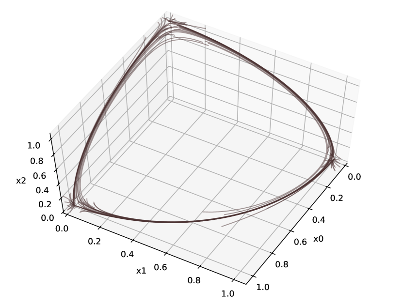
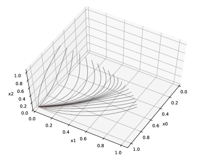
The proposed system builds upon the work on sable heteroclinic channel (SHC) networks [2, 5]. SHC networks are dynamical systems that have saddle points which can be arbitrarily connected with limit cycles (heteroclinic channels). If the saddle points are interpreted as states, then SHC networks can be understood to act like a state machine. and used as such [2]. Fig. 1 illustrates the attractor of the simplest possible SHC network coposed of three saddle points. In this paper, we additionally interpret the heteroclinic channels as representing transitions between states, propose a method to algebraically partition the state space into individual states and transitions as well as compute a phase variable for each individual transition. Further, the differential equation is modified to provide a greediness factor that modifies behavior during transitions.

.

.

.

The so-called phase-state machine combines a set of algebraic equations with existing work on stable heteroclinic channel networks (SHC). A SHC network is an attractor in a high-dimensional, continuous state space with a number of saddle points, and stable channels connecting these saddle points. The main feature of a SHC network is the straightforward computability of the system matrices from a desired state transition matrix, and that each saddle point is located along an exclusive coordinate axis. It is important to realize another property of SHC networks though: channels always lie in the plane spanned by the coordinate axes of the preceding and succeeding saddle point, i.e. any transition can be completely characterized by a rather simple projection into a two-dimensional space. In a similar fashion, activation of a state (represented by a saddle point) can be characterized by the distance along a single dimension, due to the fact that the saddle point coordinates form an orthonormal basis of the system state. This enables us to compute from the state vector two properties: the activation of any transition, and the phase of any transition.

TODO: insert phase, activation computation

II-A Formal Definition

Let $x$ be an $n$-dimensional vector that evolves according to this differential equation:

$$\dot{x}=x\circ\left(\alpha+\left(\rho_{o}+\rho_{\Delta}\circ\left(T+G\right)\right)\cdot x^{\gamma}\right)\cdot\eta(t)+\textrm{$\dot{\delta}$(t)+$\epsilon\cdot$$\mathcal{W}$(t)}$$ (1)

Compared to the equation used in [2], we added the exponent $\gamma$, explicitly introduce the state transition matrix $T$ ($T_{ji}=1$if transition $i\rightarrow j$ exists, 0 otherwise), added a “greediness” matrix $G$, and added a scalar $\eta(t)$ to adjust the speed at which $x$ evolves. The parameters $\alpha$, $\rho_{0}$and $\rho_{\Delta}$ are chosen such that $n$ saddle points occur, each one placed on its exclusive coordinate axis. The signal $\dot{\delta}$(t) is used to selectively push the system away from saddle points and $\epsilon\cdot$$\mathcal{W}$(t) adds stochastic noise with zero mean.

Matrices $\rho_{o}$and $\rho_{\Delta}$

The $n\times n$ matrices $\rho_{0}$ and $\rho_{\Delta}$ are constructed from three parameter vectors [2]: $\alpha$ (growth rates), $\beta$ (saddle point positions), and $\nu$ (saddle point shapes):

$$\rho_{o}=\left[\alpha\otimes\beta^{-1}\right]\circ\left[I-1-\alpha\otimes\alpha^{-1}\right]$$

$$\rho_{\Delta}=\left(\alpha\circ\left(1+\nu^{-1}\right)\right)\otimes\beta^{-1}$$

The matrices are chosen such that the matrix $\rho$ constructed by Eq. 5 in [2] can be computed as $\rho=-\rho_{o}-T\circ\rho_{\Delta}$. The advantage of the given formulation is that $\rho_{0}$ and $\rho_{\Delta}$ do not change when transition matrix $T$or greediness matrix $G$ is modified. For convenience, we can fix many parameters to obtain a canonical system:

$$\alpha_{i} =\alpha_{0}$$ (growth rates)

$$\beta_{i} =1.0$$ (position of saddle point)

$$\nu_{i} =1.0$$ (channel asymmetry)

To illustrate, the matrices for the system in Fig. 1 are:

$$\rho_{0}=\left[\begin{array}[]{ccc}-\alpha_{0}&-2\alpha_{0}&-2\alpha_{0}\\ -2\alpha_{0}&-\alpha_{0}&-2\alpha_{0}\\ -2\alpha_{0}&-2\alpha_{0}&-\alpha_{0}\end{array}\right]$$

$$\rho_{\Delta}=\left[\begin{array}[]{ccc}2\alpha_{0}&2\alpha_{0}&2\alpha_{0}\\ 2\alpha_{0}&2\alpha_{0}&2\alpha_{0}\\ 2\alpha_{0}&2\alpha_{0}&2\alpha_{0}\end{array}\right]$$

$$T=\left[\begin{array}[]{ccc}0&0&1\\ 1&0&0\\ 0&1&0\end{array}\right]$$

Channel location

The factor $\gamma$ determines the distance of the attractor to the vector space origin. With $\gamma=1$ channels approximately maintain constant $L^{1}$ distance (as used in [2]), whereas with $\gamma=2$ they approximately maintain constant $L^{2}$ distance (assuming a canonical system). The latter causes the attractor to lie on a hypersphere. For the canonical system, we chose $\gamma=2$.

Figure 1: Illustration of the vector field of a canonical system with three dimensions, three saddle points and three heteroclinic channels. Saddle points located at each coordinate axis, connected into a cycle $1\rightarrow 2\rightarrow 3\rightarrow 1$.

II-B Activations and Phases

The SHC network provides the notion of states (saddle points) and transitions (stable heteroclinic channels). In order to algebraically partition the vector space of $x$ into regions for each state and each possible transition, we can leverage two mathematical properties of the system.

First, the coordinate vectors of each state/saddle point form an orthonormal basis. From this follows that the channels are located on the plane spanned by the basis vectors of predecessor and successor state, as can also be seen in Fig. 1.

Second, the coordinate vector of each state is sparse, all but one coordinates are zero. From this follows that functions specific to a state or transition can be computed from specific elements of $x$.

Activation values of states and transitions

From these insights we can devise an “activation” value for each transition $i\rightarrow j$, based on its respective successor and predecessor coordinate values and the norms of $x$:

$$\Lambda^{\textrm{transitions}} = \frac{16\cdot x\otimes x\cdot|x^{2}|}{\left(x\otimes\boldsymbol{1}+\boldsymbol{1}\otimes x\right)^{4}+|x|^{4}}\circ T$$ (2)

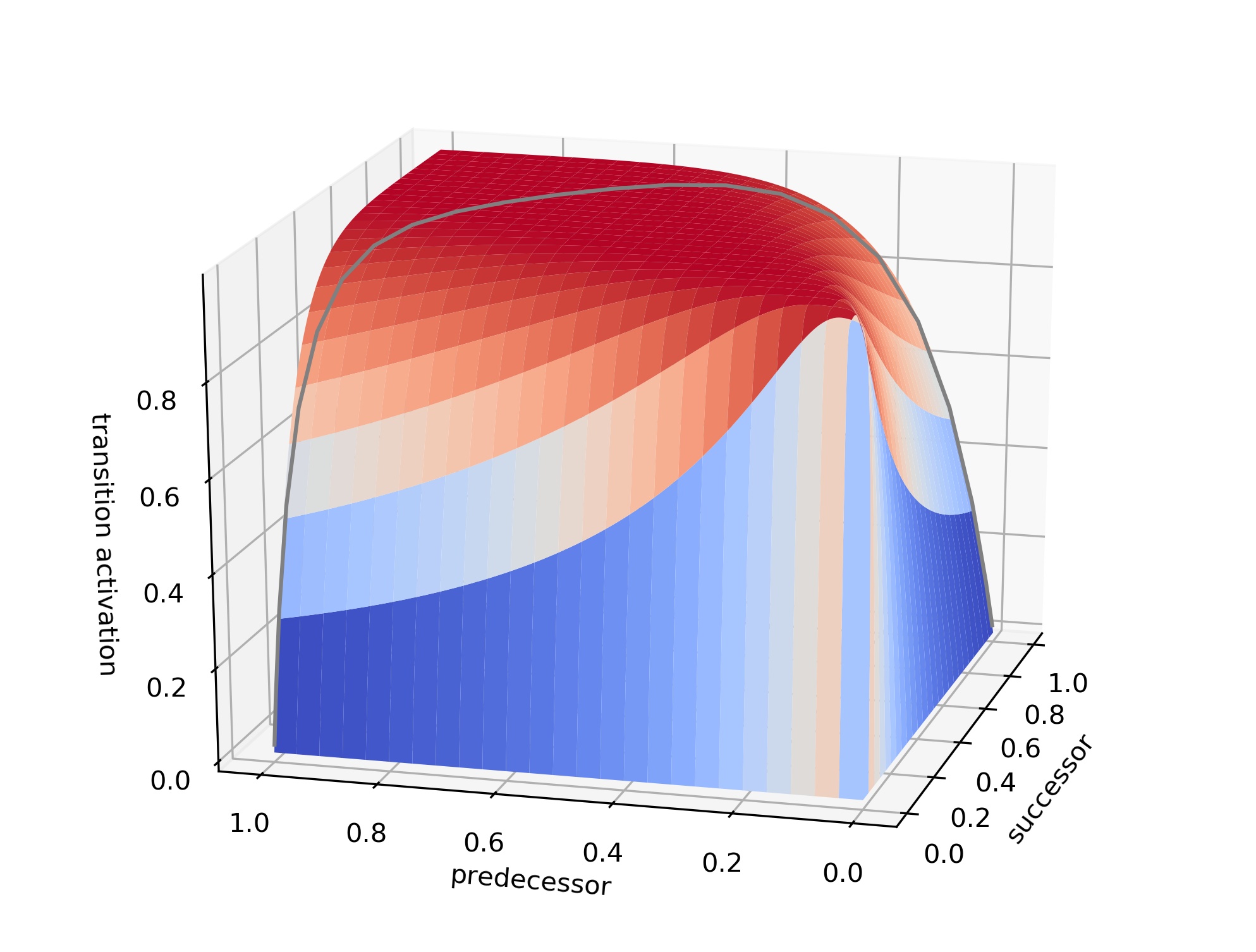
The function is chosen such that elements are limited to the range of $[0.0\ldots 1.0]$, and invariant to scaling $x$. Fig.2 illustrates the function value for a single active transition $i\rightarrow j$ w.r.t. coordinates $x_{i}$ and $x_{j}$. $\Lambda^{\textrm{transitions}}$ is sparse in the sense that only few transitions are active at any time. If more than one transition is active, then $\sum\Lambda^{\textrm{transitions}}\approx 1.0$ (for systems with $\gamma=2$). Because of this, $\Lambda^{\textrm{transitions}}$ can also be understood as a weight matrix.

Figure 2: Illustration of activation $\Lambda_{ji}$ in the plane of the related transition $i\rightarrow j$. Grey line indicates the location of heteroclinic channel for $\gamma=2$.

For the states, activation is computed from the residual of the transition activations, so that all activation values sum up to $1.0$. Additionally, $x$ is squared to ensure sparseness of the state activation values and hence mutual exclusiveness:

$$\lambda^{\textrm{states}} = x^{2}\cdot(1-\frac{\sum\Lambda^{\textrm{transitions}}}{|x^{2}|})$$ (3)

And as the diagonal of $\Lambda^{\textrm{transitions}}$ is semantically not meaningful, we can combine all transition and state activations into a single activation matrix $\Lambda$:

$$\Lambda_{ji}=\begin{cases}\lambda_{ji}^{\textrm{transitions}}&j\neq i\\ \lambda_{i}^{\textrm{states}}&j=i\end{cases}$$

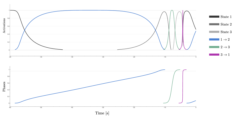
Fig. 4 shows an example of the resulting set of activation values for the minimal three-state system illustrated in Fig. 1 (using $\alpha_{0}=10$, $\dot{\delta}=5\cdot 10^{-5}$) .

Figure 3: Illustration of phase $\Psi_{ji}$ in the plane of the related transition $i\rightarrow j$. Grey line indicates the location of heteroclinic channel for $\gamma=2$.

Transition Phases

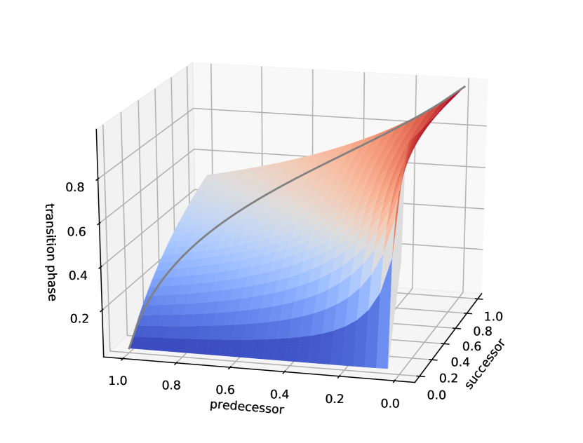
Different to (markovian) states, transitions have a notion of time and progress, i.e. they posses a phase. As channels are located on a two-dimensional plane spanned by two coordinate axes, we can compute a phase for each possible transition $i\rightarrow j$:

$$\Phi_{ji} = \frac{|x_{j}|}{|x_{i}|+|x_{j}|}$$ (4)

The shape of the function is illustrated in 2, and yields values in the range $\left[0\ldots 1\right]$. Note that $\Phi_{ji}$ is only meaningful when transition $i\rightarrow j$ is active, i.e. when $|x_{i}|+|x_{j}|\gg 0$. Fig. 4 illustrates the phase over time.

Figure 4: Activations and phases resulting from the 3-state system shown in Fig. 1. For clarity, values are not drawn when the related activation is less than 0.01.

II-B1 Composition of Motion

So far, we established a dynamical system that provides us with a consistent set of activation values for transitions and states, and with phases for transitions. Eqs. 2 and 3 are chosen such that $\sum\Lambda=1$, therefore $\Lambda$ can be directly used for weighted averaging of control goals associated with each state and each transition. In terms of control, states and transitions have to be treated differently though. States are phase-less, so we can only associate static control goals with them. Transitions, on the other hand, have a phase, so we can also associate phase-parameterized movement primitives with them, such as DMPs [4, 6] and ProMPs [4], or simply planned trajectories. For the full system demonstration, we use the ProMP framework to learn and reproduce movements during transitions. In order to enable composition using the mixing method for ProMPs [4], state goals are defined as static normal distribution over position and velocity. It is important to note that even though usually only one or two control goals are activated, multiple goals may be active, e.g. when competing transitions (with common predecessor state) become active, or when subsequent transitions are blended into each other because of large values in $\dot{\delta}$.

II-C Inputs to influence system behavior

Terms of Eq. 1 is chosen such that some of them can be used as inputs to effect certain behaviors. The transition matrix T is used to define which transitions exist, and can be updated during execution of the system, if desired. Matrix G is used to adjust the behavior for active, competing transitions and for pausing or aborting transitions. Vector $\dot{\delta}$ determines, when a state is left and which transition(s) is activated. The factor $\eta$ speeds up or slows down the system dynamics, which can be used for e.g. synchronization by entraining.

Causing transitions

When the system is exactly on a saddle point, e.g. $x=(1,0,0)$, then the system can potentially stay in this state forever. In order to cause a transition, a small positive velocity bias $\dot{\delta_{j}}$ can be added, which pushes the system towards successor state $j$, or a negative $\dot{\delta_{j}}$ to avoid it. Sometimes though, this level of granularity is not enough, and we want to set the velocity bias for each transition specifically. We can define an input biases matrix $B$ where each element $B_{ji}$ corresponds to the bias towards state $j$ in state $i$. A resolved vector $\dot{\delta}$ can then be computed with $\Lambda$ :

$$\dot{\delta}=\left(\Lambda\circ B\right)\cdot x$$ (5)

The matrix B elements are the equivalent of control switch conditions in hybrid automata, i.e. B can be used to synchronize on events and to select one out of several successor states. But it also can be used to implement timeout conditions by using small values whose effect gradually accumulates. Indeed, B was set to a small positive value for generating for generating timeouts to the states in Figs. 1 and4. If needed, bias values for specific durations can be estimated analytically [2].

Another option to cause transitions is to add stochastic velocity noise via $\epsilon$. In contrast to $\dot{\delta}$ it will cause the system to transition after a random amount of time. This might be useful in some interaction scenarios (e.g. avoiding synchronous access to a resource, or exploratory behavior). Usually though, $\epsilon=0$.

Transition Velocity

A key advantage of the proposed system to hybrid automata is the ability to continuously adjust the speed of a movement. In prior work, velocity was adjusted by modifying the growth rate $\alpha$ [2]. Unfortunately though, stability considerations limit the range of values that can be assigned to each $\alpha_{j}$. By using the activation matrix $\Lambda$ though, we can modify the growth rate (and thus speed of evolution) for each region in vector space independently:

$$\eta=2^{\sum\Lambda\circ A}$$ (6)

Matrix $A$ contains factors for speeding up or slowing down each transition and state relative to the “default” speed defined by $\alpha_{o}$. The proposed approach, works well across several orders of magnitude as it does not warp the saddle points. Unmodified system behavior is obtained by setting $A=0$.

Figure 5: Example of transition velocities ranging 3 orders of magnitude. $A_{21}=-5$, $A_{32}=0$,$A_{13}=5$

Decisiveness and Hesitation

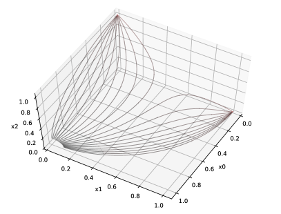
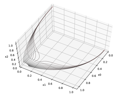
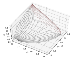
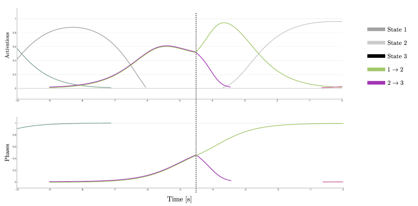
A unique feature of the proposed system is the ability to transition from a predecessor state into the direction of several successor states at once, by setting positive biases for transitions with common predecessor. The attractor shape forces a decision at some point though and only one transition completes, i.e. the system converges to one heteroclinic channel, a behavior which ensures the mutual exclusivity of states. The dynamic behavior of two competing heteroclinic channels is illustrated in Fig. 6a. Depending on $\dot{\delta}$, the system state $x$ will first progress in a specific direction on the hypersphere, but then trajectories will converge towards either of the succeeding saddle points.

Figure 6: Effect of changing the greediness parameter uniformly on two competing transitions $0\rightarrow 1$ and $0\rightarrow 2$. (a) The system can be reluctant to choose (original SHC behavior, $g=[1,1,1]$). (b) It can be very decisive ($g=[8,8,8]$). (c) With $g=[0,0,0]$ ongoing transitions are halted. (d) With negative values transitions are aborted and the the system returns to the predecessor state 0 ($g=[-2,-2,-2]$).

It turns out that this “greediness” of successor states can be consistently modified by introducing a matrix $G$ in Eq. 1:

$$G=\left[T\circ\overrightarrow{G}-\overrightarrow{G}^{T}\circ T^{T}\right]-\left[TT^{T}\circ(1-I)\right]\circ\overleftrightarrow{G}$$

The matrix $\overleftrightarrow{G}$ encodes competitive greediness, i.e. mutual inhibition between competing successor states, while $\overrightarrow{G}$ encodes greediness w.r.t. the preceding state. When $\overleftrightarrow{G}=0$ and $\overrightarrow{G}=0$ the system behaves as in [2] and Fig. 6a, when $\overrightarrow{G_{ji}}=-1$, the gradient for the channel $i\rightarrow j$ is compensated, i.e. the transition halts. If $\overrightarrow{G}=\overleftrightarrow{G}$, then For simplicity we can define a single greediness vector $g$ with values for each (successor) state, from which we can construct both matrices:

$$\overrightarrow{G}_{ji}=\begin{cases}-0.5&g_{j}<-1\\ \frac{g_{j}-1}{2}&else\\ 0&g_{j}>1\end{cases}$$

and

$$\overleftrightarrow{G}_{ji}=1.5\cdot\frac{g_{j}-1}{2}-0.5\cdot\frac{g_{i}-1}{2}$$

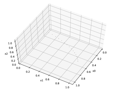
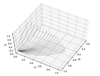
The equations are chosen such that the behavior of the original SHC network is retrieved with $g_{j}=\text{1}$. (“default” greediness). With $g_{j}=0$ (Fig. 7a), the system will completely halt ongoing transitions towards state $j$, i.e. the gradient along the heteroclinic channel drops to zero. With negative $g_{j}$ (Fig. 7b), the gradient along the heteroclinic channel reverses, which moves the system back to the preceding state.

The speed of transitions are not increased beyond the default speed because $\overrightarrow{G}$ is clamped. Values beyond $|g_{j}|>1$ therefore only increases the competition between successor states. The net effect is, that for large values of $g$ , the system becomes very decision-happy (Fig. 6b vs. Fig. 6b) and tries to converge towards a single transition early, while for low values of $g$, the system is reluctant to decide. This effect can be used to modulate the ambiguity of movements. If two expressive movements are associated with two competing transitions, then large values of $g$ will cause the system to avoid mixing movements, which maintains their expressiveness. If $g$ is small then movements are mixed according to the accumulated $\dot{\delta}$, creating an ambiguous motion.

Figure 7: Effects of non-positive greediness. (a) $g=[1,0,0]$ halts ongoing transitions. (b) $g=[1,-1,-1]$ reverses ongoing transitions (c) $g=[1,-2,-2]$ reverses ongoing transitions and additionally balances them.

Reconsidering Decisions

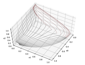
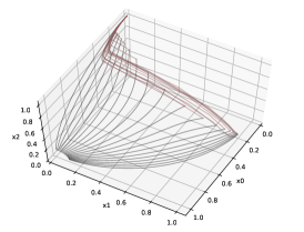
The greediness can not only be used to alter mixing behavior during transitions, but it can also be used to make the system reconsider the successor state it is converging to. The ratio of $\frac{g_{2}}{g_{1}}$ for two competing successor states determines where the system bifurcates. By altering the ratio, a system that previously was set to converge towards one state can be made to converge towards another state. This effectively enables us to reconsider earlier decisions on which successor state to converge to. For illustration, Fig. 8 shows three systems where during a transition, elements of $g$ are changed asymmetrically. Depending on the absolute values, the system can be made to “reluctantly” move towards the new desired successor state (Fig. 8a), to respond gradually depending on how certain it was before (Fig. 8b), or to aggressively “backtrack” (Fig. 8c).

Figure 8: Asymmetric greediness can be used to “reconsider” earlier decisions between competing transitions. Black lines indicate where $g=[1,1,1]$, with different initial biases during predecessor state activation. Red lines indicate where (f.l.t.r) $g=[0,0,1]$, $g=[0,0.5,2]$, $g=[0,-1,20]$.

It should be noted, that the greediness input provides a powerful method to alter the “flavor” of transitions, while keeping the overall state graph intact (as expressed by the transition matrix T).

Figure 9: Effect of changing greediness on phases and activations. The dotted line indicates where $g=[1,1,1]$ changes to $g=[1,5,0]$.

III Experiments

In order to demonstrate the capability of the proposed system to quickly react to perceptual input, and to generate legible motion, all while maintaining a simple state graph abstraction of an interaction, we chose to apply it for a handover task. In this task, a robot arm picks up an object from a table surface, and then hands it over to a human interaction partner standing nearby. The object can be handed over to the left or the right hand of the human

illustrated the wealth of behaviors that we can implement with non-instant transitions between markovian states, such as modulating decisiveness/hesitation, reconsideration of decisions after the transition has started, and even aborting ongoing transitions. In the context of human-robot interaction, these behaviors enable communication by body language for negotiating interaction alternatives and for synchronizing actions. In order to demonstrate the feasibility of the system to generate legible motions, and to implement negotiability of interaction alternatives, we implement a handover task. The robot picks up an object and then has two options: it can give the object either into the right hand or the left hand of the human interaction partner. The human can indicate his/her preference by extending or retracting the respective hand, giving four possible options. If no hand is extended, then the human does not communicate any preference. If either hand is extended, the preference is clear. If both hands are extended, the robot interprets it as an offer to choose; either hand is fine, and the robot should choose swiftly. Additionally, we use the distance and orientation of the humans torso to gauge their readiness for interaction. If a human turns away or walks away, an ongoing reachout by the robot needs to be aborted.

The proposed system provides a consistent method to generate legible mixtures of phase based motions such as probabilistic movement primitives [4] or dynamic movement primitives[6]

IV Discussion

IV-A Conclusions

The paper presented a novel method to structure and execute robot motion, which is especially suited for implementing human-robot interaction based on body motion. The paper analyzed properties and parameters of the proposed system and related modulations to human-interpretable qualities such as decisiveness and hesitation, which can be used to negotiate decisions faster and more effectively than relying on turn-based interaction.

References