Thermal-FIST: A package for heavy-ion collisions and hadronic equation of state

Abstract

Thermal-FIST is a C++ package designed for convenient general-purpose physics analysis within the family of hadron resonance gas (HRG) models. This mainly includes the statistical analysis of particle production in heavy-ion collisions and the phenomenology of hadronic equation of state. Notable features include fluctuations and correlations of conserved charges, effects of probabilistic decay, chemical non-equilibrium, and inclusion of van der Waals hadronic interactions. Calculations are possible within the grand canonical ensemble, the canonical ensemble, as well as in mixed-canonical ensembles combining the canonical treatment of certain conserved charges with the grand-canonical treatment of other conserved charges. The package contains a fast thermal event generator, which generates particle yields in accordance with the HRG chemistry, and particle momenta based on the Blast Wave model. A distinct feature of this package is the presence of the graphical user interface frontend – QtThermalFIST – which is designed for fast and convenient general-purpose HRG model applications.

Program summary

Program Title: Thermal-FIST, version 1.2
Licensing provisions: GPLv30
Programming language: C++
Computer: any with a C++ compiler and, optionally, the Qt5 framework for the GUI frontend
Operating system: cross-platform, tested on Linux Ubuntu 16.04, 18.04; Mac OS X Yosemite, Microsoft Windows 10; Android 8, 9
External routines: Eigen template library for the linear algebra routines [1], MINUIT2 package from CERN ROOT [2], Mersenne Twister random number generator [3], Qt5 framework [4] (for the GUI only), QCustomPlot Qt widget [5] (for the GUI only)
Nature of problem:
The HRG model and its various modifications constitute a common framework used for modeling of the hadronic equation of state and particle production in heavy-ion collisions. Even the simplest versions of the HRG model require careful considerations of the many details, including the resonance decay feed-down, implementation of charge conservation constraints relevant for heavy-ion collisions, chemical non-equilibrium effects. A notable extra effort is required in order to treat the fluctuations and correlations of various charges charges, which presently are being extensively studied in the heavy-ion collision experiments and lattice QCD calculations. The inclusion of hadronic interactions, modeled by an excluded-volume (EV) or a van der Waals (vdW) type framework, additionally requires a numerical solution to a system of many transcendental equations.
Solution method:
The Thermal-FIST package contains a class-based library which calculates relevant HRG observables for a specified setup. The setup includes a particle list, usually to be supplied with an external file, an HRG model specification (statistical ensemble, van der Waals interaction parameters, etc.), a set of thermal parameters, and conservation laws constraints. Whenever necessary, the systems of transcendental equations are solved numerically with the Broyden’s method. The package includes a fitter for extracting thermal parameters from hadron yield data through the $\chi^{2}$ minimization. The HRG model based Monte Carlo event generator is a complementary feature to analytic calculations. A general-purpose thermal analysis is made maximally convenient with QtThermalFIST – a GUI frontend based on the Qt framework where all typical calculations, such as the properties of the equation of state or the thermal fits, can be straightforwardly performed.
Additional comments:
If the EV/vdW interactions are present, exact analytic calculations are presently only possible within the grand canonical ensemble. Approximate calculations are possible for the strangeness-canonical ensemble on the condition that strange particles form a small subsystem relative to the total system. Effects of probabilistic decays on fluctuation observables are generally included only up to the moments of the 2nd order. The only exception is the ideal HRG model in the grand canonical ensemble, where these effects are included up to the moments of the 4th order. On the other hand, the Monte Carlo event generator is not constrained by the above restrictions.
Running time:
Depending on the specific task, calculation times may vary from milliseconds (an evaluation of thermodynamic functions within the ideal HRG model in the GCE) to several minutes (a thermal fit with sophisticated features such as energy-dependent widths, van der Waals interactions, or exact charge conservation). The thermal event generator takes few milliseconds to generate an event with about a thousand particles in the GCE. Event generation in the CE is considerably slower and depends on the rejection sampling rate realized for the given setup.

1 Introduction

The abundant hadron production in heavy-ion collision reactions has long been treated in the framework of the thermal-statistical models [1, 2, 3, 4, 5, 6, 7, 8, 9, 10]. Such a description assumes emission of particles from a thermally and chemically equilibrated source created in these reactions. Fitting the observed yields of stable hadrons allows to determine the thermal parameters, corresponding to the so-called chemical freeze-out stage of the collision. In most cases, the ideal hadron resonance gas (Id-HRG) model has been used, and a surprisingly good description of many experimental hadron yield data from heavy-ion collisions have been achieved within this simple approach for a broad range of collision energies, ranging from moderate energies at the SchwerIonen-Synchrotron (SIS) to the highest energy of the Large Hadron Collider (LHC) (see, e.g., Refs. [11, 12, 13] for an overview).

HRG-type models also play an important role in the phenomenology of the QCD equation of state. The Id-HRG model is a popular choice for describing the low temperature, confined phase of QCD. At temperatures between $T\sim 100-150$ MeV and at zero chemical potential, the Id-HRG model indeed appears to reproduce many lattice QCD observables [14, 15, 16, 17].

Several implementations of the Id-HRG model exist on the market, including SHARE [18, 19, 20], THERMUS [21], and THERMINATOR [22, 23].

In many applications, significant deviations from the ideal gas picture can be expected. Extensions of the ideal gas picture have been discussed mostly within the excluded volume (EV) HRG model [24, 25, 26], where the effects of repulsive hadronic interactions at short distances are introduced (see, e.g., [27] for recent developments). Another extension is the quantum van der Waals (QvdW) model [28, 29, 30], which allows to include both the repulsive and attractive interactions between hadrons. Recently, repulsive interactions have received renewed interest in the context of lattice QCD data on fluctuations of conserved charges. It was indicated that large deviations of several fluctuation observables from the Id-HRG baseline are captured by HRG models with repulsive baryon-baryon interactions [29, 31, 32, 33]. The Thermal-FIST package presented here allows to calculate thermodynamic features and fluctuation observables within a HRG with arbitrary attractive and repulsive QvdW parameters characterizing interactions between each type of hadron species.

Possible effects of chemical non-equilibrium for light, strange, and/or charm quarks in heavy-ion collisions have been studied in the framework of the Id-HRG model within the SHARE package [11, 34]. The Thermal-FIST package allows to study the chemical non-equilibrium effects simultaneously with the effects of EV/vdW interactions or exact charge conservation within the canonical ensemble.

Recent thermal model applications also include the description of the measurements of multiplicity fluctuations [35, 36, 37, 38]. Treatment of probabilistic decays [39] and hadronic interactions [36] is important in such applications, and it is included into the Thermal-FIST package.

The applications of the Thermal-FIST package which can be found in the literature include chemical freeze-out analysis in proton-proton [40, 41] and nucleus-nucleus collisions [42, 43, 44], influence of the EV interactions on thermal fits [45, 46, 47, 27] and equation of state [48, 49, 32, 33], Monte Carlo analysis of EV effects in the canonical ensemble [50], effects of the vdW interactions between baryons and nuclear liquid-gas transition on various observables [29, 51, 30, 52, 53], and thermal production of light nuclei [54, 55].

2 Hadron resonance gas

2.1 Ideal HRG

In the simplest setup, the thermodynamics of hadronic phase is described by a multi-component, ideal gas of point-like hadrons – the Id-HRG model. In the grand canonical ensemble (GCE) formulation of the Id-HRG model there are no correlations between different hadronic species. Thus, the pressure is given by

$$p(T,\mu)=\sum_{i}p_{i}^{\rm id}(T,\mu_{i}),$$ (1)

where the sum goes over all hadron species included in the model, $p^{\rm id}_{i}(T,\mu_{i})$ is the pressure of the ideal Fermi or Bose gas at the corresponding temperature and chemical potential for species $i$:

$$p^{\rm id}_{i}(T,\mu_{i})=\frac{d_{i}}{6\pi^{2}}\int_{0}^{\infty}\frac{k^{4}dk}{\sqrt{k^{2}+m_{i}^{2}}}\left[\exp\left(\frac{\sqrt{k^{2}+m_{i}^{2}}-\mu_{i}}{T}\right)+\eta_{i}\right]^{-1}~{},$$ (2)

where $d_{i}$ and $m_{i}$ are, respectively, the spin degeneracy factor and mass of hadron species $i$, and where $\eta_{i}$ equals +1 for fermions, -1 for bosons, and 0 for the Boltzmann approximation.

Other thermodynamic quantities are given by expressions similar to (1): a sum over the corresponding ideal gas quantities for all hadron species. The particle density of hadron species $i$ is $n_{i}^{\rm id}(T,\mu_{i})$, i.e. it is simply given by the ideal gas relation for species $i$:

$$n^{\rm id}_{i}(T,\mu_{i})=\frac{\partial p^{\rm id}_{i}(T,\mu_{i})}{\partial\mu_{i}}=\frac{d_{i}}{2\pi^{2}}\int_{0}^{\infty}k^{2}dk\left[\exp\left(\frac{\sqrt{k^{2}+m_{i}^{2}}-\mu_{i}}{T}\right)+\eta_{i}\right]^{-1}~{},$$ (3)

while the energy density is $\varepsilon(T,\mu)=\sum_{i}\varepsilon_{i}^{\rm id}(T,\mu_{i})$ with

$$\varepsilon^{\rm id}_{i}(T,\mu_{i})=\frac{d_{i}}{2\pi^{2}}\int_{0}^{\infty}k^{2}\,dk\,\sqrt{k^{2}+m_{i}^{2}}\left[\exp\left(\frac{\sqrt{k^{2}+m_{i}^{2}}-\mu_{i}}{T}\right)+\eta_{i}\right]^{-1}~{}.$$ (4)

Within the GCE formulation, all conserved charges, such as baryonic number $B$, electric charge $Q$, strangeness $S$, and charm $C$, are conserved on average. For the chemical equilibrium case these average values are regulated by the corresponding independent chemical potentials: $\mu_{B}$, $\mu_{Q}$, $\mu_{S}$, and $\mu_{C}$. The chemical potential of the $i$th hadron species is thus determined as

$$\mu_{i}\ =\ B_{i}\,\mu_{B}\,+\,S_{i}\,\mu_{S}\,+\,Q_{i}\,\mu_{Q}\,+\,C_{i}\,\mu_{C}$$ (5)

with $B_{i}=0,\,\pm 1$, $S_{i}=0,\,\pm 1,\,\pm 2,\,\pm 3$, $Q_{i}=0,\,\pm 1,\,\pm 2$, and $C_{i}=0,\,\pm 1,\,\pm 2$, being the corresponding conserved charges of the $i$th hadron: baryon number, strangeness, electric charge, and charm.

2.2 Chemical non-equilibrium and fugacity factors

The assumption of full chemical equilibrium can be relaxed in the heavy-ion collision applications of the HRG model. This is usually done by introducing additional fugacity factors which regulate the absolute abundances of quarks of different flavor [56, 11], initially introduced as phenomenological parameters [57, 58]. In this case, the Boltzmann factors in Eqs. (2)-(4) are modified to

$$e^{\mu_{i}/T}\to e^{\mu_{i}/T}\,\gamma_{q}^{|q_{i}|}\,\gamma_{S}^{|S_{i}|}\,\gamma_{C}^{|C_{i}|}\quad\text{[or }\mu_{i}\to\mu_{i}+T\,\log(\gamma_{q}^{|q_{i}|}\,\gamma_{S}^{|S_{i}|}\,\gamma_{C}^{|C_{i}|})\text{]},$$ (6)

where $|q_{i}|$, $|S_{i}|$, and $|C_{i}|$ correspond, respectively, to the absolute light, strange, and charm quark content of hadron $i$, and where $\gamma_{q}$, $\gamma_{S}$, and $\gamma_{C}$ are parameters which regulate deviations from chemical equilibrium in the light, strange, and charm quark sectors, respectively. $\gamma_{i}=1$ corresponds to the chemical equilibrium scenario for the corresponding quark flavor sector.

2.3 Excluded-volume corrections

The repulsive interactions between hadrons can be modeled by an excluded volume correction of the van der Waals type, whereby the volume available for hadrons to be created and move in is reduced by the sum of all their eigenvolumes. Such a correction was first studied in the hadronic equation of state in Refs. [59, 60, 61, 62, 63]. A thermodynamically consistent procedure for a single-component gas was first formulated in Ref. [24].

It should be noted that an excluded-volume correction is only an effective approach to treat repulsive interactions between hadrons. A common (and simplest) assumption is the constant eigenvolume parameter for all hadronic species [64]. A more realistic approach is to allow the possibility for different hadrons to have different eigenvolumes [25, 26]. Such an approach, however, is incomplete. For instance, it is not possible to take into account the expected differences between baryon-baryon and baryon-antibaryon interactions [65] within such a model. Therefore, each pair of hadron species can be characterized by its own “excluded volume” parameter [66] in the most general case.

All of the above options are considered and implemented in the Thermal-FIST package.

2.3.1 Diagonal EV model

In the Diagonal EV-HRG (DEV-HRG) model [25, 26], each hadron is assigned an excluded-volume parameter $v_{i}$. It is common to characterize the excluded-volume parameter $v_{i}$ with the effective hard-core radius $r_{i}$, by using the classical relation $v_{i}=(16\pi/3)\,r_{i}^{3}$. The excluded volume correction leads to the transcendental equation for the system pressure,

$$p(T,\mu)=\sum_{i}\,p^{\rm id}(T,\mu_{i}^{*}),\qquad\mu_{i}^{*}=\mu_{i}-v_{i}\,p,$$ (7)

which is solved numerically. The numerical solution is obtained in Thermal-FIST using the Broyden’s method [67].

Other thermodynamic functions are then obtained from the standard thermodynamic relations:

$$n_{i}(T,\mu) \equiv\left(\frac{\partial p}{\partial\mu_{i}}\right)_{T}=\frac{n_{i}^{\rm id}(T,\mu_{i}^{*})}{1+\sum_{j}v_{j}n_{j}^{\rm id}(T,\mu_{j}^{*})},$$ (8)

$$s(T,\mu) \equiv\left(\frac{\partial p}{\partial T}\right)_{\mu}=\frac{\sum_{i}s_{i}^{\rm id}(T,\mu_{i}^{*})}{1+\sum_{j}v_{j}n_{j}^{\rm id}(T,\mu_{j}^{*})},$$ (9)

$$\varepsilon(T,\mu) \equiv Ts+\sum_{i}\mu_{i}\,n_{i}-p=\frac{\sum_{i}\varepsilon_{i}^{\rm id}(T,\mu_{i}^{*})}{1+\sum_{j}v_{j}n_{j}^{\rm id}(T,\mu_{j}^{*})}.$$ (10)

2.3.2 Non-diagonal EV model

The repulsive interactions in the Non-Diagonal EV-HRG (NDEV-HRG) model [66, 46, 27] are characterized by the matrix $\tilde{b}_{ij}$ of the excluded volume type parameters, which characterize the repulsive interactions for each pair of particle species. The total pressure is partitioned into the sum of “partial” pressures,

$$p(T,\mu)=\sum_{i}p_{i}(T,\mu),$$ (11)

which are determined by the following system of transcendental equations:

$$p_{i}(T,\mu)=p_{i}^{\rm id}(T,\mu_{i}^{*}),\qquad\mu_{i}^{*}=\mu_{i}-\sum_{j}\widetilde{b}_{ij}\,p_{j},\qquad i=1,\ldots,f.$$ (12)

The solution to Eq. (12) at given $T$ and $\mu$ is obtained numerically in Thermal-FIST, using the multi-dimensional Broyden’s method.

The particle number densities $n_{i}\equiv(\partial p/\partial\mu_{i})_{T}$ are found as the solution to the system of linear equations

$$\sum_{j}[\delta_{ij}+\tilde{b}_{ji}\,n_{i}^{\rm id}(T,\mu_{i}^{*})]\,n_{j}=n_{i}^{\rm id}(T,\mu_{i}^{*}),\qquad i=1\ldots f.$$ (13)

The entropy and energy densities are given by

$$s(T,\mu) =\sum_{i}(1-\sum_{j}\tilde{b}_{ji}\,n_{j})\,s^{\rm id}_{i}(T,\mu_{i}^{*}),$$ (14)

$$\varepsilon(T,\mu) =\sum_{i}(1-\sum_{j}\tilde{b}_{ji}\,n_{j})\,\varepsilon^{\rm id}_{i}(T,\mu_{i}^{*}).$$ (15)

Parameters $\tilde{b}_{ij}$ can be chosen arbitrarily for each pair of particle species. They need not to be symmetric. One possibility is the classical picture of a multi-component gas of hard spheres, where each species is characterized by the hard-core radius $r_{i}$ and where $\tilde{b}_{ij}$ are given by

$$\widetilde{b}_{ij}=\frac{2\,b_{ii}\,b_{ij}}{b_{ii}+b_{jj}}\qquad\text{with}\qquad b_{ij}=\frac{2\pi}{3}\,(r_{i}+r_{j})^{3}.$$ (16)

The NDEV-HRG model reduces to the DEV-HRG model in the partial case $\widetilde{b}_{ij}\equiv v_{i}$.

2.4 Quantum van der Waals model

The presence of both, the short-range repulsive and the intermediate/long range attractive interactions between hadrons can be treated in the framework of the Quantum van der Waals (QvdW) equation [28], extended to multiple components present in a HRG [29, 30]. This QvdW-HRG model is defined by the following pressure function

$$p(T,\mu)=\sum_{i}p^{\rm id}_{i}(T,\mu_{i}^{*})-\sum_{i,j}\,a_{ij}\,n_{i}\,n_{j}.$$ (17)

The particle number densities, $n_{i}$, satisfy the system of linear equations

$$\sum_{j}[\delta_{ij}+\tilde{b}_{ji}\,n_{i}^{\rm id}(T,\mu_{i}^{*})]\,n_{j}=n_{i}^{\rm id}(T,\mu_{i}^{*}),\qquad i=1\ldots f,$$ (18)

while the shifted chemical potentials, $\mu_{i}^{*}$, satisfy the system of transcendental equations

$$\mu^{*}_{i}+\sum_{j}\tilde{b}_{ij}\,p^{*}_{j}-\sum_{j}(a_{ij}+a_{ji})\,n_{j}=\mu_{i}~{},\quad i=1,\ldots,f~{}.$$ (19)

The pressure, $p(T,\mu)$, at a given temperature $T$ and chemical potentials $\mu$ is determined by first solving numerically the system of equations (19) for $\mu_{i}^{*}$ and then plugging in the result into Eq. (17).

The entropy and energy densities are given as

$$s(T,\mu) =\sum_{i}(1-\sum_{j}\tilde{b}_{ji}\,n_{j})\,s^{\rm id}_{i}(T,\mu_{i}^{*}),$$ (20)

$$\varepsilon(T,\mu) =\sum_{i}(1-\sum_{j}\tilde{b}_{ji}\,n_{j})\,\varepsilon^{\rm id}_{i}(T,\mu_{i}^{*})-\sum_{i,j}a_{ij}\,n_{i}\,n_{j}~{}.$$ (21)

The parameters $\tilde{b}_{ij}$ correspond to the repulsive vdW interactions, and they have the same physical meaning as in the NDEV-HRG model. The parameters $a_{ij}$ correspond to the attractive vdW interactions between hadron species $i$ and $j$, modeled in the mean-field approximation. The QvdW-HRG model reduces to the NDEV-HRG model for the case $a_{ij}\equiv 0$.

The QvdW-HRG model permits the inclusion into the HRG model of the basic features of nuclear matter, in particular, the nuclear liquid-gas phase transition and the associated criticality. The critical point of nuclear matter was shown to be important for the fluctuation observables in heavy-ion collisions [68, 29, 69, 53].

2.5 Finite resonance widths

The finite widths of the resonances may play an important role for some applications of the HRG model. These can be taken into account in a simplified way, by adding an additional integration into Eqs. (2)-(4) over the resonance masses [70, 21]

$$\int dk\,\to\,\int_{m_{i}^{\rm min}}^{m_{i}^{\rm max}}dm\,\rho_{i}(m)\,\int dk\,,$$ (22)

where $\rho_{i}(m)$ is the mass distribution for resonance $i$, taken either in the relativistic Breit-Wigner form,

$$\rho_{i}(m)=A_{i}\,\frac{2\,m\,m_{i}\,\Gamma_{i}(m)}{(m^{2}-m_{i}^{2})^{2}+m_{i}^{2}\,[\Gamma_{i}(m)]^{2}},$$ (23)

or the nonrelativistic Breit-Wigner form,

$$\rho_{i}(m)=A_{i}\,\frac{1}{(m-m_{i})^{2}+[\Gamma_{i}(m)]^{2}/4}.$$ (24)

Here $A_{i}$ is determined from the normalization condition $\int_{m_{i}^{\rm min}}^{m_{i}^{\rm max}}dm\,\rho_{i}(m)=1$.

There are different possibilities for the choice of $m_{i}^{\rm min}$ and $m_{i}^{\rm max}$, as well as for the mass-dependence of the width $\Gamma_{i}(m)$. Two options are implemented in Thermal-FIST: (1) integration in the truncated interval, defined by $m_{i}^{\rm min}=\max(m_{i}-2\Gamma_{i},m_{i}^{\rm thr})$ and $m_{i}^{\rm max}=m_{i}+2\Gamma_{i}$, with energy independent widths [70, 21], and (2) integration in the full interval, defined by $m_{i}^{\rm min}=m_{i}^{\rm thr}$ and $m_{i}^{\rm max}=\infty$, with energy dependent widths. Here $m_{i}^{\rm thr}$ is the threshold mass. More details about the different options and their implementation can be found in Ref. [43].

2.6 Feeddown from resonance decays

Applications of the HRG model to particle production must take into account the feeding from decays of unstable particles (resonances) to the final hadron yields measured in experiments. Feeding from resonance decays gives dominant contribution in many cases, as much as 70% of all final pions may come from resonance decays [21]. This is illustrated in Fig. 1, which shows different feeddown contribution to the total yields of pions and protons, evaluated in the Id-HRG model at $T=155$ MeV, $V=4000$ fm³, and zero chemical potentials.

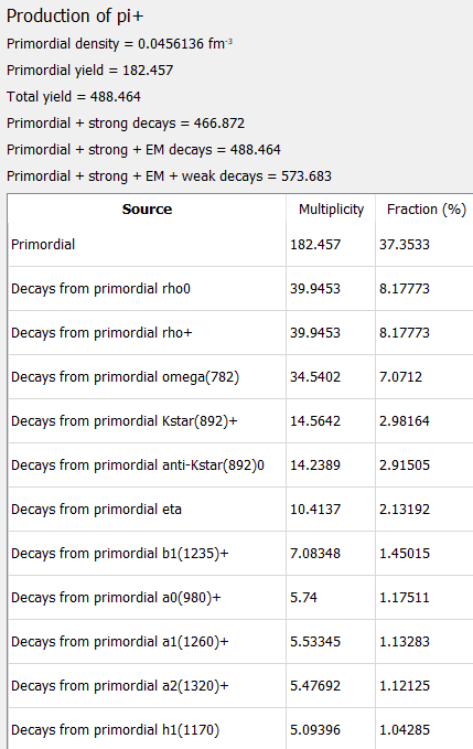
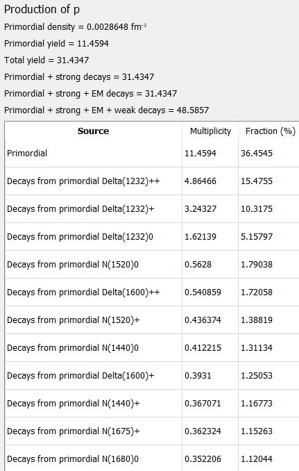
Figure 1: Screen grabs from the QtThermalFIST GUI program showing differential yield contributions to the final yields of $\pi^{+}$ (left panel) and protons (right panel), evaluated in the Id-HRG model at $T=155$ MeV, $V=4000$ fm³, and zero chemical potentials.

The final mean multiplicity $\langle N_{i}\rangle$ of $i$th particle species is calculated in the HRG model as a sum of the primordial mean multiplicity $\langle N^{*}_{i}\rangle\equiv n_{i}\,V$ and resonance decay contributions as follows

$$\langle N_{i}\rangle~{}=~{}\langle N^{*}_{i}\rangle~{}+~{}\sum_{R}\langle n_{i}\rangle_{R}\,\langle N^{*}_{R}\rangle~{},$$ (25)

where $\langle n_{i}\rangle_{R}$ is the average number of particles of type $i$ resulting from decay of resonance $R$. $\langle n_{i}\rangle_{R}$ includes contribution from both, the direct decays of resonance $R$ resulting in the production of hadron $i$, as well as the contributions resulting from the chain of decays via lower-mass resonances. Note that for energy-dependent resonance widths the relation (25) is modified to reflect energy dependent branching ratios, see Ref. [43] for details.

The exact decay feeddown chain for each hadron yield should be matched to the relevant experimental conditions. By default, the hadrons which decay strongly or electromagnetically are marked unstable in Thermal-FIST. It is also possible, for each hadron species, to evaluate final yields which include contributions from strong decays only, from strong and electromagnetic decays, from strong, electromagnetic and weak decays, or in accordance with manually set particle stability flags that define the feeddown.

2.7 Correlations, fluctuations and susceptibilities

2.7.1 Conserved charges

Fluctuations and correlations of conserved charges are characterized by the corresponding susceptibilities

$$\chi_{lmnk}^{BSQC}~{}=~{}\frac{\partial^{l+m+n+k}p/T^{4}}{\partial(\mu_{B}/T)^{l}\,\partial(\mu_{S}/T)^{m}\,\partial(\mu_{Q}/T)^{n}\,\partial(\mu_{C}/T)^{k}}~{}\,.$$ (26)

These susceptibilities are useful, as they carry information about finer details of the equation of state, they can be obtained in the lattice QCD simulations, and they can also be measured in heavy-ion collisions, although in many cases proxy observables have to be used.

In the most general case, the derivatives defining a particular $\chi_{lmnk}^{BSQC}$ can be evaluated numerically by calculating the pressure function at different values of chemical potentials. The diagonal susceptibilities of an arbitrary conserved charge (which can be, e.g., some linear combination of $B$, $S$, $Q$, and $C$), can be calculated within Thermal-FIST analytically up to the 4th order. This analytic procedure is described in [30] for the QvdW-HRG model, all other models included are obtained as partial cases of the QvdW-HRG model.

2.7.2 Hadron yield fluctuations and probabilistic decays

Fluctuations and correlations of hadron numbers can also be considered. A hadron yield is not a conserved quantity, and, therefore, it cannot be calculated from first-principles using lattice QCD. On the other hand, in contrast to the conserved charges, hadron yields are quantities which are directly measured in heavy-ion collision experiments, and they are readily available for calculation in a HRG approach.

The cumulants $\chi_{k}^{i}$ of the primordial hadron number distributions, $N_{i}^{*}$, can be calculated by taking the derivatives with respect to the chemical potential $\mu_{i}$ of hadron specie $i$. In particular

$$\chi_{2}^{i} \equiv\frac{\partial^{2}(p/T^{4})}{\partial(\mu_{i}/T)^{2}}=\frac{1}{VT^{3}}\,\langle(\Delta N_{i}^{*})^{2}\rangle,$$ (27)

$$\chi_{3}^{i} \equiv\frac{\partial^{3}(p/T^{4})}{\partial(\mu_{i}/T)^{3}}=\frac{1}{VT^{3}}\,\langle(\Delta N_{i}^{*})^{3}\rangle,$$ (28)

$$\chi_{4}^{i} \equiv\frac{\partial^{4}(p/T^{4})}{\partial(\mu_{i}/T)^{4}}=\frac{1}{VT^{3}}\,\langle(\Delta N_{i}^{*})^{4}\rangle_{c}=\frac{1}{VT^{3}}\,[\langle(\Delta N_{i}^{*})^{4}\rangle-3\,\langle(\Delta N_{i}^{*})^{2}\rangle^{2}],$$ (29)

where $\chi_{k}^{i}$ are expressed here through the central moments of the primordial hadron number distribution. $\chi_{k}^{i}$ are evaluated in Thermal-FIST in the same way as the fluctuations of conserved charges.

The two-particle correlator $\langle\Delta N_{i}^{*}\Delta N_{j}^{*}\rangle$ for the primordial hadron yields $N_{i}^{*}$ and $N_{j}^{*}$ is given by the mixed derivative

$$\frac{1}{VT^{3}}\,\langle\Delta N_{i}^{*}\Delta N_{j}^{*}\rangle=\frac{\partial^{2}(p/T^{4})}{\partial(\mu_{i}/T)\,\partial(\mu_{j}/T)}~{},$$ (30)

while the higher-order correlations are obtained in a similar fashion.

The correlations and fluctuations in final hadron yields are affected by the probabilistic decays of the resonances. The variance of the final hadron yield $N_{i}$ is calculated as follows [71, 72, 73, 36]

$$\langle(\Delta N_{i})^{2}\rangle =\langle(\Delta N_{i}^{*})^{2}\rangle+\,\sum_{R}\,\langle N_{R}^{*}\rangle\,\langle(\Delta n_{i})^{2}\rangle_{R}$$

$$\quad+2\,\sum_{R}\,\langle\Delta N_{i}^{*}\Delta N_{R}^{*}\rangle\,\langle n_{i}\rangle_{R}+\sum_{R,R^{\prime}}\,\langle\Delta N_{R}^{*}\,\Delta N_{R^{\prime}}^{*}\rangle\,\langle n_{i}\rangle_{R}\,\langle n_{i}\rangle_{R^{\prime}}.$$ (31)

Here $\langle(\Delta n_{i})^{2}\rangle_{R}$ is the variance of the number of hadrons of type $i$ which result from the chain of probabilistic decays of the resonance $R$.

The higher-order fluctuations of final hadron yields are considered in Thermal-FIST for the Id-HRG model only. The third and fourth cumulants in this model read [39]

$$\langle(\Delta N_{i})^{3}\rangle =\langle(\Delta N_{i}^{*})^{3}\rangle+\sum_{R}\langle(\Delta N_{R}^{*})^{3}\rangle\langle n_{i}\rangle_{R}^{3}+3\sum_{R}\langle(\Delta N_{R}^{*})^{2}\rangle\langle n_{i}\rangle_{R}\langle(\Delta n_{i})^{2}\rangle_{R}$$

$$\quad+\sum_{R}\langle N_{R}^{*}\rangle\langle(\Delta n_{i})^{3}\rangle_{R}\,,$$ (32)

$$\langle(\Delta N_{i})^{4}\rangle_{c} =\langle(\Delta N_{i}^{*})^{4}\rangle_{c}+\sum_{R}\langle(\Delta N_{R}^{*})^{4}\rangle_{c}\langle n_{i}\rangle_{R}^{4}+6\sum_{R}\langle(\Delta N_{R}^{*})^{3}\rangle\langle n_{p}\rangle_{R}^{2}\langle(\Delta n_{i})^{2}\rangle_{R}$$

$$\quad+\sum_{R}\langle(\Delta N_{R}^{*})^{2}\rangle\bigg{[}3\,\langle(\Delta n_{i})^{2}\rangle_{R}^{2}+4\,\langle n_{i}\rangle_{R}\langle(\Delta n_{i})^{3}\rangle_{R}\bigg{]}$$ (33)

$$\quad+\sum_{R}\langle N_{R}^{*}\rangle\langle(\Delta n_{i})^{4}\rangle_{R,c}\,.$$ (34)

Here $\langle(\Delta n_{i})^{3}\rangle_{R}$ and $\langle(\Delta n_{i})^{4}\rangle_{R,c}=\langle(\Delta n_{i})^{4}\rangle_{R}-3\,\langle(\Delta n_{i})^{2}\rangle_{R}^{2}$ are, respectively, the third and fourth cumulants of the distribution of the number of hadrons of type $i$ which result from the chain of probabilistic decays of the resonance $R$.

2.8 Canonical ensemble

The exact conservation of conserved charges can be enforced within the canonical thermodynamics. The effects of exact charge conservation influence hadron yields in small systems, typically when the number of hadrons carrying a particular conserved charge is of the order of unity or smaller. The exact charge conservation also affects strongly the fluctuations of hadron numbers, even in the thermodynamic limit.

Analytic calculations in the canonical ensemble are restricted in Thermal-FIST to the Id-HRG model.

2.8.1 Full canonical ensemble

The canonical ensemble treatment implies exact conservation of the corresponding conserved charges. The partition function of the Id-HRG in the canonical ensemble for fixed baryon number $B$, electric charge $Q$, strangeness $S$, and charm $C$, reads [70, 74]

$$\mathcal{Z}(B,Q,S,C) =\int\limits_{-\pi}^{\pi}\frac{d\phi_{B}}{2\pi}\int\limits_{-\pi}^{\pi}\frac{d\phi_{Q}}{2\pi}\int\limits_{-\pi}^{\pi}\frac{d\phi_{S}}{2\pi}\int\limits_{-\pi}^{\pi}\frac{d\phi_{C}}{2\pi}~{}e^{-i\,(B\phi_{B}+Q\phi_{Q}+S\phi_{S}+C\phi_{C})}$$

$$\quad\times\exp\left[\sum_{j}\sum_{n=1}^{\infty}z_{j,n}\,e^{i\,n\,(B_{j}\phi_{B}+Q_{j}\phi_{Q}+S_{j}\phi_{S}+C_{j}\phi_{C})}\right].$$ (35)

Here

$$z_{j,n}=(\mp 1)^{n+1}\,\gamma_{q}^{|q_{j}|}\,\gamma_{S}^{|S_{j}|}\,\gamma_{C}^{|C_{j}|}\,\frac{d_{j}\,V_{c}}{2\pi^{2}}\,\frac{T\,m^{2}}{n^{2}}\,K_{2}\left(n\frac{m}{T}\right),$$ (36)

with $V_{c}$ being the canonical correlation volume, i.e. the volume over which the exact conservation is enforced. The mean primordial multiplicity for species $j$ is given by

$$\langle N_{j}\rangle_{ce}=\sum_{n=1}^{\infty}\frac{Z(B-n\,B_{j},Q-n\,Q_{j},S-n\,S_{j},C-n\,C_{j})}{Z(B,Q,S,C)}\,n\,z_{j,n}.$$ (37)

Similar expressions exist for other thermodynamic functions, as well as for fluctuations and correlations of particle numbers [72]. Note that all the above relations include the effects of quantum statistics, given by the summation over $n$. This sum is truncated at a sufficiently large $n_{\rm max}$ value in calculations. The calculations proceed by evaluating the partition functions, given by Eq. (2.8.1), through a numerical integration. For the case when both, quantum statistical effects are neglected for baryons and when there are no particles in the list with $|B_{j}|>1$, the integration over $\phi_{B}$ is performed analytically, using the method of Ref. [75]. This allows to significantly speed up the calculations.

The inclusion of quantum statistics and fluctuations is a new element compared to the functionality of the presently available other open source packages. Most packages do not include the canonical ensemble at all. One exception is THERMUS [21], where calculations are, however, restricted to the case of Boltzmann statistics and where it is not possible to consider particles which have a baryon number $|B_{j}|>1$.

It is also possible to selectively treat certain conserved charges grand-canonically, while preserving the canonical treatment for other conserved charges. To remove the canonical treatment of a certain conserved charge, for instance the baryon charge $B$, one removes the integration over $\phi_{B}$ in Eq. (2.8.1), sets $\phi_{B}$ to zero in the integrand, and adds the baryon number fugacity factor into the expression (36) for the one-particle partition function. The selective canonical treatment of conserved charges can clarify the role of canonical effects for different conserved charges in a given setup.

The canonical ensemble implementation works reliably and fast when the system volume or conserved charges are sufficiently small. This covers the typical cases where the effects of exact charge conservation on mean hadron multiplicities are significant.

2.8.2 Strangeness/charm canonical ensemble

The abundances of hadrons carrying strangeness produced in intermediate-energy heavy-ion collisions are notably smaller than those of light flavored hadrons. The abundances of charm hadrons are even smaller. Therefore, in many cases it is sufficient to implement the canonical treatment of strangeness or charm only, while preserving the grand canonical treatment of baryon number and electric charge. The canonical treatment of strangeness is achieved in the so-called strangeness-canonical ensemble (SCE). In principle, the full canonical ensemble implementation as described above provides such a functionality. In some cases, however, the system volume can be large, and the above implementation can be inefficient. Therefore, here we consider an alternative approach to calculate the partition functions in Eq. (2.8.1). Assuming the Boltzmann statistics for strange particles, the SCE partition function is expressed as the sum over the Bessel functions [76]

$$\mathcal{Z}(S)=\mathcal{Z_{\rm NS}}\,\sum_{k=-\infty}^{\infty}\,\sum_{p=-\infty}^{\infty}\,a_{3}^{p}\,a_{2}^{k}\,a_{1}^{-2k-3p-S}\,I_{k}(x_{2})\,I_{p}(x_{3})\,I_{-2k-3p-S}(x_{1}).$$ (38)

Here $\mathcal{Z_{\rm NS}}$ is the grand-canonical partition function of the subsystem consisting of non-strange particles, and

$$a_{i}=\sqrt{S_{i}/S_{-i}},\qquad x_{i}=2\sqrt{S_{i}\,S_{-i}},\qquad i=1,2,3$$

with $S_{i}=\sum_{j\in(S_{j}=i)}\langle N_{j}^{\rm gce}\rangle$ being the cumulative mean multiplicity of all particle carrying strangeness $i$ calculated in the grand canonical ensemble.

The canonical treatment of charm here assumes that there are no multi-charmed particles in the particle list and that the system is net charm free, which is sufficient for most applications. The yields of charmed hadrons in the charm-canonical ensemble (CCE) are then calculated as follows

$$\langle N_{i}^{\rm ce}\rangle=\langle N_{i}^{\rm gce}\rangle\,\frac{I_{1}(\sum_{j\in C}\langle N_{j}^{\rm gce}\rangle)}{I_{0}(\sum_{j\in C}\langle N_{j}^{\rm gce}\rangle)},\qquad i\in C.$$ (39)

2.9 Thermal fits

Perhaps the most common application of the HRG model is fitting the hadron yield data from relativistic heavy-ion collisions – the thermal fits. Such an approach assumes thermal and (partial) chemical equilibrium between all stable hadrons and all resonances at the so-called “chemical freeze-out” stage of a heavy-ion reaction. The HRG model fits are performed by minimizing the value

$$\frac{\chi^{2}}{N_{\rm dof}}~{}=~{}\frac{1}{N_{\rm dof}}\sum_{i=1}^{N}\frac{\left(N_{i}^{\rm exp}~{}-~{}N_{i}^{\rm HRG}\right)^{2}}{\sigma_{i}^{2}}~{},$$ (40)

where $N_{i}^{\rm exp}$ and $N_{i}^{\rm HRG}$ are the experimental and calculated in the HRG hadron multiplicities, respectively; $N_{\rm dof}$ is the number of degrees of freedom, that is the number of the data points minus the number of fitting parameters; and $\sigma_{i}^{2}=(\sigma_{i}^{syst})^{2}+(\sigma_{i}^{stat})^{2}$ is the sum of the squares of the statistical and systematic experimental errors. Note that $N_{i}^{\rm HRG}$ is the total hadron yield, including the resonance feeddown, calculated in accordance with Eq. (25) and using the appropriate feeddown flags. $N_{i}$ in Eq. (40) can also represent a ratio of two yields. Thermal-FIST employs the MINUIT2 package [77] for the $\chi^{2}$ minimization procedure.

In the simplest setup, corresponding to the full chemical equilibrium in the grand canonical ensemble, there are only three fit parameters: the temperature $T$, the baryonic chemical potential $\mu_{B}$, and the system volume parameter $V$. The electric charge and strangeness chemical potentials $\mu_{Q}$ and $\mu_{S}$ are not fitted. Instead, at each fixed temperature $T$ and baryochemical potential $\mu_{B}$, the $\mu_{Q}$ and $\mu_{S}$ are determined in a unique way in order to satisfy two conservation laws given by the “initial” conditions: the electric-to-baryon charge ratio of $Q/B=0.4$, and the vanishing net strangeness $S=0$. These two conditions are relevant if pre-freezeout radiation is neglected. Otherwise, $\mu_{S}$ and/or $\mu_{Q}$ can also be considered as additional fit parameters. For completeness, Thermal-FIST also allows to constrain the baryochemical potential $\mu_{B}$ to a fixed entropy-per-baryon ratio, $S/B$.

The chemical potentials disappear in the canonical ensemble formulation. In this case, the total baryon, electric charge, strangeness, and charm numbers appear instead, these are fixed by the “initial” conditions.

Some modifications, such as chemical under- or over-saturation of the light, strange, and/or charm quarks can also introduce additional parameters, $\gamma_{q}$, $\gamma_{S}$, and $\gamma_{C}$ (see, e.g., Refs. [11, 78]).

3 Monte Carlo event generator

Thermal-FIST implements Thermal Event Generator (TEG) – a Monte Carlo generator of hadronic microstates that correspond to a particular formulation of the HRG model in grand canonical or canonical ensemble. The effects of radial flow are included in the framework of the blast wave model. Monte Carlo implementation of the probabilistic decays of the primordial resonances is also provided.

The TEG is useful for heavy-ion collision applications, as well as for calculation of observables which are otherwise problematic using the analytic methods. These include e.g., effects of radial flow and momentum cuts. Another example is the higher-order fluctuations and correlations of final hadron yields, which may include the effects of the probabilistic decays of resonances and of the residual EV/QvdW interactions between the primordial hadrons. Monte Carlo formulation also allows to study the simultaneous effects of the EV interactions and the global charge conservation, which presently cannot be done using the analytic methods.

The TEG assumes that hadrons stem from a thermally equilibrated source, i.e. they are emitted from a particular “freeze-out” hypersurface. Each point at the hypersurface is characterized by the same values of all thermal parameters of a HRG. The generation of each event consists of three steps:

1. The multiplicities of all primordial hadrons are generated from the probability distribution which corresponds to the partition function of a particular HRG model.

2. Momenta of all primordial hadrons are generated, independently for each hadron. The momentum distribution is given by the spherical or longitudinal Blast Wave model, with a kinetic freeze-out temperature parameter $T_{\rm kin}$ that can be different from the chemical freeze-out temperature $T_{\rm ch}$.

3. Probabilistic decay chain of all resonances in the system is simulated until only the stable hadrons remain (optional).

It should be noted that the TEG is a rather simplistic event generator and has certain limitations. First, the present implementation is restricted to a HRG in the Boltzmann approximation, thus, the quantum statistical effects are omitted. Second, it is also assumed that the momenta and coordinates of the thermal hadrons at freeze-out are uncorrelated. The validity of such approximation can be questioned if two-particle correlations at freeze-out, e.g. due to the EV interactions, are non-negligible. Third, the modeling of decays assumes isotropic two-body and three-body decay kinematics, but provides only an approximate treatment of the isotropic many-body (four or more) decay kinematics. Therefore, an analysis of the observables which may be sensitive to the kinematics of many-body decays should be done with care.

3.1 Multiplicity sampling

The implementation of the multiplicity sampling is done according to the procedure described in Ref. [50]. Here only the basic details are described.

3.1.1 Poisson distribution

In the simplest case one has the Id-HRG model in the grand canonical ensemble. In this case the multiplicity distribution for each hadron species is given by the Poisson distribution, i.e. all multiplicities are described by the multi-Poisson distribution:

$$\Pi(\{N_{i}\};T,V,\{\mu_{Q}\})~{}=~{}\prod_{i=1}^{f}\,\frac{\langle N_{i}\rangle^{N_{i}}}{N_{i}!}\,e^{-\langle N_{i}\rangle}~{},$$ (41)

where $\langle N_{i}\rangle\equiv\phi_{i}(T)\,e^{\mu_{i}/T}\,V$ is the mean number of hadron species $i$ in the GCE.

In the sampling procedure, first $\langle N_{i}\rangle=n_{i}\,V$ are calculated analytically, and then $\{N_{i}\}$ are generated for each event independently for each hadron species $i$ from the Poisson distribution.

3.1.2 Exact charge conservation

In the canonical ensemble all globally conserved charges are conserved exactly. In the Id-HRG model this condition modifies the multi-Poisson distribution as follows:

$$\Pi(\{N_{i}\};T,V,\{\mu_{Q}\})~{}=~{}\prod_{i=1}^{f}\,\frac{\langle N_{i}\rangle^{N_{i}}}{N_{i}!}\,e^{-\langle N_{i}\rangle}~{}\times\prod_{k=1}^{q}\delta(Q_{k}-\sum_{j=1}^{f}Q_{k}^{(j)}N_{j}),$$ (42)

where the index $k$ runs through all conserved charges in the system.

The implementation of exact charge conservation proceeds by combining the sampling from the multi-Poisson distribution with a rejection sampling. To speed up the process, we use the multi-step sampling procedure described in Ref. [79].

3.1.3 EV/QvdW interactions

A presence of the EV interactions leads to an appearance of a reduced volume in the partition function. In addition, the number of particles in the system is restricted from above, such that the total cumulative eigenvolume of all hadrons does not exceed the system volume. In the QvdW-HRG model, the presence of vdW interactions leads to the following modification of the microstate probability in the GCE (see Ref. [50] for details):

$$\Pi_{EV}(\{N_{i}\};T,V,\{\mu_{Q}\}) \propto\prod_{i=1}^{f}\,\frac{\left[(V-\sum_{j}\tilde{b}_{ji}N_{j})\,z_{i}\,e^{\mu_{i}/T}\right]^{N_{i}}}{N_{i}!}\,\exp\left(\sum_{j}\frac{a_{ij}N_{j}}{VT}N_{i}\right)$$

$$\quad\times\Theta(\{N_{i}\};V),$$ (43)

$$\Theta(\{N_{i}\};V) =\prod_{i=1}^{f}\,\theta(V-\sum_{j}\tilde{b}_{ji}N_{j})~{}.$$ (44)

The Monte Carlo procedure in this case uses the importance sampling technique. Namely, the $\{N_{i}\}$ multiplicities for each event are still generated from the multi-Poisson distribution, but each generated event is assigned a weight $w=\Pi_{\rm vdW}/\Pi$. Therefore, any observable is calculated as a weighted average. The theta function in Eq. (3.1.3) is taken into account via a rejection sampling as well: all $\{N_{i}\}$ configurations for which $\Theta(\{N_{i}\};V)$ evaluates to zero are rejected. The average multiplicities $\langle N_{i}\rangle$ used for the sampling from the auxiliary multi-Poisson distribution (41) are evaluated analytically using the GCE formulation of the QvdW-HRG model.

The multiplicity sampling for the QvdW-HRG model in the CE contains an additional rejection sampling step, as described in the previous subsection. The DEV-HRG and NDEV-HRG models follow from the QvdW-HRG model as partial cases, as elaborated in Sec. 2.4.

3.2 Momentum sampling

The thermal momenta of all the primordial hadrons are generated independently for each hadron. A possibility of collective motion at freeze-out is included in the framework of the blast-wave model. Two options are available: the spherically symmetric blast wave scenario [80], appropriate for intermediate collision energies, and the cylindrically symmetric blast wave scenario [81], which is more appropriate for high collision energies.

3.2.1 Spherically symmetric blast wave model

In the spherically symmetric blast wave model the momentum distribution is given by the Siemens-Rasmussen formula [80]:

$$\omega_{p}\frac{dN}{d^{3}p}=\tilde{N}\,e^{-\frac{\gamma\,E}{T_{\rm kin}}}\,\omega_{p}\,\left[\left(1+\frac{T_{\rm kin}}{\gamma\,\omega_{p}}\right)\frac{\sinh\alpha}{\alpha}-\frac{T_{\rm kin}}{\gamma\,\omega_{p}}\cosh\alpha\right],$$ (45)

where $\gamma=(1-\beta^{2})^{-1/2}$, $\alpha=\gamma\,\beta\,p/T_{\rm kin}$, $\beta\in[0,1)$ is the radial flow velocity parameter, and $\tilde{N}$ is the normalization constant. $T_{\rm kin}$ is the kinetic freeze-out temperature, which can be taken different from the chemical freeze-out temperature that determines the multiplicity distribution. The momentum vector $\mathbf{p}$ is considered in the spherical coordinate basis, i.e.

$$\mathbf{p}=(p\,\sin\theta_{p}\,\cos\varphi_{p},p\,\sin\theta_{p}\,\sin\varphi_{p},p\,\cos\theta_{p}).$$

The spherical coordinate angles $\varphi_{p}$ and $\theta_{p}$ are generated assuming the isotropic distribution, i.e. $\varphi_{p}$ and $\cos\theta_{p}$ are uniformly and independently distributed in the $[0,2\pi)$ and $[-1,1]$ intervals, respectively. The distribution function for $p$ follows from Eq. (45):

$$\frac{dN}{dp}=4\pi\,p^{2}\,\tilde{N}\,e^{-\frac{\gamma\,E}{T_{\rm kin}}}\,\left[\left(1+\frac{T_{\rm kin}}{\gamma\,\omega_{p}}\right)\frac{\sinh\alpha}{\alpha}-\frac{T_{\rm kin}}{\gamma\,\omega_{p}}\cosh\alpha\right].$$ (46)

For practical purposes, it is convenient to perform the following variable change

$$p=-p_{0}\,\log\xi.$$ (47)

The new variable $\xi$ takes values in the finite interval $0\leq\xi<1$, which is convenient for a numerical implementation. The distribution function of $\xi$ reads

$$\frac{dN}{d\xi}=\frac{dN}{dp}\,\left|\frac{dp}{d\xi}\right|=\frac{p_{0}}{\xi}\,4\pi\,p^{2}\,\tilde{N}\,e^{-\frac{\gamma\,E}{T_{\rm kin}}}\,\left[\left(1+\frac{T_{\rm kin}}{\gamma\,\omega_{p}}\right)\frac{\sinh\alpha}{\alpha}-\frac{T_{\rm kin}}{\gamma\,\omega_{p}}\cosh\alpha\right].$$ (48)

The function $dN/d\xi$ goes to zero at the edges of the interval $0\leq\xi<1$, and a has a maximum in-between. Therefore, the value of $\xi$ is generated using the rejection sampling technique. The value of the maximum of $dN/d\xi$ is determined using the ternary search. The $p_{0}=1$ GeV value is used in the present implementation. After the value of $\xi$ is generated, the absolute value of momentum is calculated via Eq. (47).

The above procedure is repeated for all particles in the event.

3.2.2 Cylindrically symmetric blast wave model

The momentum distribution in the cylindrically symmetric blast wave model is given by [81]:

$$\omega_{p}\frac{dN}{d^{3}p} =\tilde{N}\,m_{T}\,\int_{-\eta_{\rm max}}^{\eta_{\rm max}}d\eta\cosh(y-\eta)\,\int_{0}^{1}\tilde{r}\,d\tilde{r}$$

$$\quad\times\exp\left[-\frac{m_{T}\,\cosh\rho\,\cosh(y-\eta)}{T_{\rm kin}}\right]\,I_{0}\left(\frac{p_{T}\sinh\rho}{T_{\rm kin}}\right),$$ (49)

where $m_{T}=\sqrt{p_{T}^{2}+m^{2}}$ is the transverse mass, $y=\displaystyle\frac{1}{2}\log\frac{\omega_{p}-p_{z}}{\omega_{p}+p_{z}}$ is the longitudinal rapidity, $\rho=\tanh^{-1}\beta_{r}$, and $\beta_{r}=\beta_{s}\tilde{r}^{n}$ is the transverse flow velocity profile, $\eta_{\rm max}$ is the longitudinal rapidity cutoff. $\beta_{s}$ is the transverse flow velocity at the surface. The mean transverse flow velocity is $\langle\beta_{T}\rangle=\frac{2}{2+n}\,\beta_{s}$. The particle three-momentum is parameterized as $\mathbf{p}=(p_{T}\,\cos\varphi_{p},p_{T}\sin\varphi_{p},m_{T}\sinh y)$.

Due to the azimuthal symmetry, the azimuthal angle $\varphi_{p}$ is distributed uniformly in the interval $[0,2\pi)$, and it is independent of $p_{T}$ and $y$ .

The distribution function for the transverse momentum $p_{T}$ reduces to [81]:

$$\frac{dN}{dp_{T}}\propto p_{T}\,m_{T}\,\int_{0}^{1}\tilde{r}\,d\tilde{r}\,I_{0}\left(\frac{p_{T}\sinh\rho}{T_{\rm kin}}\right)\,K_{1}\left(\frac{m_{T}\cosh\rho}{T_{\rm kin}}\right).$$ (50)

The $p_{T}$ value is generated using the change of variable $p_{T}=-p_{0}\,\log\xi$, and the rejection sampling technique for the generation of $\xi$, using the same method as described in the previous subsection for the Siemens-Rasmussen formula.

The rapidity distribution at a fixed value of $p_{T}$ follows from Eq. (3.2.2):

$$\frac{dN}{dy}(y~{}|~{}p_{T}) \propto\int_{-\eta_{\rm max}}^{\eta_{\rm max}}d\eta\cosh(y-\eta)\,\int_{0}^{1}\tilde{r}\,d\tilde{r}$$

$$\quad\times\exp\left[-\frac{m_{T}\,\cosh\rho\,\cosh(y-\eta)}{T_{\rm kin}}\right]\,I_{0}\left(\frac{p_{T}\sinh\rho}{T_{\rm kin}}\right).$$ (51)

The value of $y$ is generated from Eq. (3.2.2) using the rejection sampling technique.

4 Thermal-FIST structure and implementation

Thermal-FIST is implemented as a C++ library of classes and functions. The applications of the package proceed by linking the ThermalFIST library within a C++ program (macro), which performs the needed task.

The library documentation is available online [82]. Here only the basic structure is described.

4.1 Base classes

4.1.1 IdealGasFunctions module

Calculation of thermodynamic properties of an ideal gas in the GCE forms the basis of all HRG calculations in Thermal-FIST. These are given as functions of the temperature $T$, the chemical potential $\mu$, the particle mass $m$, the internal degeneracy factor $d$, and the statistics $\eta$. Here $\eta=+1$ corresponds to the Fermi-Dirac statistics, $\eta=-1$ corresponds to the Bose-Einstein statistics, and $\eta=0$ corresponds to the Maxwell-Boltzmann statistics.

These functions are implemented in the IdealGasFunctions module, and include pressure, particle number density, energy density, entropy density, scalar density, and the leading four particle number susceptibilities $\chi_{k}$.

The calculations within the Maxwell-Boltzmann statistics ($\eta=0$) use known analytical expressions involving the modified Bessel functions. For example, the pressure reads

$$p^{\rm id}_{MB}(T,\mu)=\frac{d\,m^{2}\,T^{2}}{2\pi^{2}}\,K_{2}(m/T).$$ (52)

Similar expressions exist for all other ideal gas functions.

There are two options for the numerical calculations of the ideal quantum gas functions ($\eta=\pm 1$): (i) using the cluster expansion technique, (ii) using the numerical integration with Gauss-Laguerre quadratures (the default method).

Cluster expansion

The first method uses the cluster expansion of an ideal quantum gas. The calculations proceed by calculating the truncated cluster expansion, e.g., the pressure is calculated as

$$p^{\rm id}_{q}(T,\mu)\simeq\frac{d\,m^{2}\,T^{2}}{2\pi^{2}}\sum_{k=1}^{k_{\rm max}}\frac{(-\eta)^{k+1}}{k^{2}}\,e^{k\,\mu/T}\,K_{2}(k\,m/T),$$ (53)

similar expressions are used for other thermodynamic functions. The value of $k_{\rm max}$ can be regulated, it should be sufficiently large for accurate calculations. Setting $k_{\rm max}=1$ one recovers the Maxwell-Boltzmann statistics. Note that cluster expansion formally diverges if $\mu>m$. Therefore, this method should not be used for calculating the Fermi-Dirac functions for $\mu>m$, and extra care taken for the case $\mu\lesssim m$.

Numerical integration

The numerical integration method proceeds by evaluating the integrals numerically, with the help of quadratures. First, the integrals are written in the dimensionless form,

$$p^{\rm id}_{q}(T,\mu) =\frac{d}{6\pi^{2}}\,\int_{0}^{\infty}\,dk\,\frac{k^{4}}{\sqrt{m^{2}+k^{2}}}\,\left\{\exp\left(\frac{\sqrt{m^{2}+k^{2}}-\mu}{T}\right)+\eta\right\}^{-1}$$

$$=\frac{d\,T^{4}}{6\pi^{2}}\,\int_{0}^{\infty}\,d\tilde{k}\,\frac{\tilde{k}^{4}}{\sqrt{\tilde{m}^{2}+\tilde{k}^{2}}}\,\left\{\exp\left(\sqrt{\tilde{m}^{2}+\tilde{k}^{2}}-\tilde{\mu}\right)+\eta\right\}^{-1},$$ (54)

where $\tilde{k}=k/T$, $\tilde{m}=m/T$, and $\tilde{\mu}=\mu/T$.

For $\mu<m$, the calculations proceed by applying the 32-point Gauss-Laguerre quadrature to the dimensionless integral in Eq. (4.1.1).

For $\mu>m$, the Bose-Einstein integrals are divergent. The Fermi-Dirac integrals, however, are convergent and can be computed. The numerical accuracy of the above-described method, however, is usually unsatisfactory in such a case. Therefore, for calculating the Fermi-Dirac integrals at $\mu>m$, Eq. (4.1.1) is rewritten as follows [83, 84]:

$$p^{\rm id}_{\rm FD}(T,\mu) \stackrel{{\scriptstyle\mu>m}}{{=}}-\frac{d\,T^{4}}{6\pi^{2}}\,\int_{0}^{\tilde{p}_{F}}\,d\tilde{k}\,\frac{\tilde{k}^{4}}{\sqrt{\tilde{m}^{2}+\tilde{k}^{2}}}\,\left\{\exp\left(\tilde{\mu}-\sqrt{\tilde{m}^{2}+\tilde{k}^{2}}\right)+1\right\}^{-1}$$

$$\quad+\frac{d\,T^{4}}{6\pi^{2}}\,\int_{\tilde{p}_{F}}^{\infty}\,d\tilde{k}\,\frac{\tilde{k}^{4}}{\sqrt{\tilde{m}^{2}+\tilde{k}^{2}}}\,\left\{\exp\left(\sqrt{\tilde{m}^{2}+\tilde{k}^{2}}-\tilde{\mu}\right)+1\right\}^{-1}$$

$$\quad+\frac{d\,T^{4}}{6\pi^{2}}\left[\tilde{\mu}\,\tilde{p}_{F}^{3}-\frac{3}{4}\,\tilde{p}_{F}^{4}\,\psi(\tilde{m}/\tilde{p}_{F})\right].$$ (55)

Here $\tilde{p}_{F}=\sqrt{\tilde{\mu}^{2}-\tilde{m}^{2}}$ and

$$\psi(x)=\left(1+\frac{x^{2}}{2}\right)\sqrt{1+x^{2}}-\frac{x^{4}}{2}\ln\left(\frac{1+\sqrt{1+x^{2}}}{x}\right).$$ (56)

The first integral in Eq. (4.1.1) is evaluated using the 32-point Gauss-Legendre quadrature, while the second integral in Eq. (4.1.1) is evaluated using the 32-point Gauss-Laguerre quadrature.

Expressions similar to Eq. (4.1.1) are obtained for other quantities using the standard thermodynamic relations.

4.1.2 ThermalModelParameters

The HRG model parameters are kept in the ThermalModelParameters structure. Each implementation of the HRG model has this structure, which contains the values of thermal parameters used in calculations. List of all parameters is presented in Table 1.

Table 1: List of HRG model parameters contained in the ThermalModelParameters structure.

Parameter	Unit	Notes
Temperature ($T$)	GeV	–
Baryon chemical potential ($\mu_{B}$)	GeV	Not in CE
Electric chemical potential ($\mu_{Q}$)	GeV	Not in CE
Strangeness chemical potential ($\mu_{S}$)	GeV	Not in CE/SCE
Charm chemical potential ($\mu_{C}$)	GeV	Not in CE/SCE/CCE
$\gamma_{q}$	–	–
$\gamma_{S}$	–	–
$\gamma_{C}$	–	–
Volume ($V$)	fm3	–
Canonical volume ($V_{c}$)	fm3	In CE, SCE, CCE
Baryon charge ($B$)	–	CE only
Electric charge ($Q$)	–	CE only
Strangeness ($S$)	–	CE, SCE
Charm ($C$)	–	CE, CCE

4.1.3 ThermalParticle class

The ThermalParticle class contains all information about the properties of a particular hadron species in the hadron list. This includes the Particle Data Group (PDG) code, the mass, the degeneracy, the type of quantum statistics, the quantum numbers, absolute quark contents, and, if applicable, the decay channels and the width.

The class also provides various methods. The calculation of the ideal gas functions is performed through the Density method. These calculations take into account a possible additional integration due to a finite width. Other methods provide setting of various options, including whether the integrals are evaluated using the cluster expansion or the numerical integration, the number of terms in the cluster expansion (if this method is used), the shape and the prescription used to treat the finite resonance widths. More details can be found in the online documentation [82], in particular in the annotated ThermalParticle.h source file.

4.1.4 ThermalParticleSystem class

The ThermalParticleSystem class contains the list of particles to be used in calculations, represented by a vector of ThermalParticle objects, one per each particle species.

The particle list is usually provided from an external file. The LoadList method of the class loads the particle list from an external file. The external file which contains the particle list has a format of a table, where each row correspond to a single particle specie. Each column in the table corresponds to a particular hadron property. List of all columns is provided in Table 2.

Table 2: List of hadron properties contained in an input file.

Column	Value type	Description
PDG ID	long long	PDG code
Name	string	Particle name
Stability flag	bool	Stability w.r.t decays
Mass [GeV]	double	Particle mass
Degeneracy	double	Internal degeneracy factor
Statistics	int	Fermi (+1), Bose (-1), Boltzmann (0)
$B$	int	Baryon number
$Q$	int	Electric charge
$S$	int	Strangeness
$C$	int	Charm
$n_{|S|}$	double	Absolute strange quark content
$n_{|C|}$	double	Absolute charm quark content
Width [GeV]	double	Resonance width
Threshold [GeV]	double	Threshold mass

4.1.5 ThermalModel classes

Implementation of the different HRG models is contained in classes starting with the prefix ThermalModel.

ThermalModelBase

ThermalModelBase is the base class for all ThermalModel classes. This is an abstract class containing fields and methods common for an arbitrary variant of HRG model. The exact implementation of some of these methods can be different in different versions of HRG, and is given in the corresponding derived classes. The ThermalModelBase class instance contains a pointer to a ThermalParticleSystem object containing the particle list, and a ThermalModelParameters structure with all the thermal model parameters. Both are provided during the creation of the ThermalModelBase instance. Some of the important methods of the class include:

• Methods to set the various thermal model parameters. The list is given in Table 3.

• SetUseWidth method to specify the treatment of finite resonance widths.

• ConstrainMuB(bool), ConstrainMuQ(bool), ConstrainMuS(bool),
  and ConstrainMuC(bool) methods to define whether the values of the corresponding chemical potentials should be constrained by, respectively, a fixed entropy per baryon ratio $S/B$, electric-to-baryon charge ratio $Q/B$, zero strangeness and zero charm.

• ConstrainChemicalPotentials() procedure constrains, if required, the chemical potentials $\mu_{B}$, $\mu_{Q}$, $\mu_{S}$, and/or $\mu_{C}$.

• CalculatePrimordialDensities() procedure calculates the primordial hadronic densities for current values of the thermal parameters. This is the main method were most calculations take place.

• CalculateFeeddown() procedure calculates various feeddown contributions to final yields (densities) of hadrons after the primordial densities were computed.

• double GetDensity(int PDGID, Feeddown::Type feeddown) returns the calculated density for a particle with the given PDG code and feeddown. The feeddown parameter can be 0 (primordial density), 1 (with feeddown according to the stability flags), 2 (with strong/electromagnetic/weak decay feeddown), 3 (with strong/electromagnetic decay feeddown), and 4 (with strong decay feeddown). This method should only be called after the primordial and final densities were calculated.

Table 3: List of the ThermalModelBase methods to set HRG parameters.

Method	Parameter	Notes
SetTemperature	$T$	–
SetBaryonChemicalPotential	$\mu_{B}$	–
SetElectricChemicalPotential	$\mu_{Q}$	–
SetStrangenessChemicalPotential	$\mu_{S}$	–
SetCharmChemicalPotential	$\mu_{Q}$	–
SetGammaq	$\gamma_{q}$	–
SetGammaS	$\gamma_{S}$	–
SetGammaC	$\gamma_{C}$	–
SetVolume	$V$	–
SetVolumeRadius	$R$	Sets $V=(4/3)\pi R^{3}$
SetCanonicalVolume	$V_{c}$	CE, SCE, CCE
SetCanonicalVolumeRadius	$R_{c}$	Sets $V_{c}=(4/3)\pi R_{c}^{3}$
SetBaryonCharge	$B$	For CE only
SetElectricCharge	$Q$	For CE only
SetStrangeness	$S$	CE, SCE
SetCharm	$C$	CE, CCE

Classes which implement the different variants of the HRG model inherit from the ThermalModelBase class and are listed in Table 4. More details about the usage of the ThermalModel classes can be found in the corresponding source files and in the annotated sample routines in the src/examples folder.

Table 4: List of classes inheriting from the ThermalModelBase class and the corresponding HRG model.

Class	HRG model variant	Ensemble
ThermalModelIdeal	Id-HRG	GCE
ThermalModelDiagonalEV	Diagonal EV-HRG	GCE
ThermalModelCrosstermsEV	Non-diagonal EV-HRG	GCE
ThermalModelVDW	QvdW-HRG	GCE
ThermalModelCanonical	Id-HRG	CE/GCE
ThermalModelCanonicalStrangeness	Id-HRG	SCE
ThermalModelCanonicalCharm	Id-HRG	CCE

4.2 ThermalModelFit class

The ThermalModelFit class implements routines related to the thermal fitting of hadron yields and/or yield ratios. The class instance contains a pointer to the ThermalModelBase class instance, provided on object initialization, as well as the set of parameters for fitting, and the data to fit.

The list of all possible fit parameters is shown in Table 5. If the parameters $\mu_{Q}$, $\mu_{S}$, or $\mu_{C}$ are not fitted, then they are constrained by the corresponding $Q/B$ ratio and strangeness/charm neutrality conditions. Obviously, (some of) these parameters are not used in the fit also if CE/SCE/CCE ensemble is employed where these parameters do not appear at all.

Table 5: List of fit parameters in a thermal model fit, their default values and fit flags

Parameter	Default
	value	fit flag
$T$	0.150 GeV	true
$\mu_{B}$	0	true
$\mu_{Q}$	0	false
$\mu_{S}$	0	false
$\mu_{C}$	0	false
$\gamma_{q}$	1	false
$\gamma_{S}$	1	false
$\gamma_{C}$	1	false
$R$	8 fm	true
$R_{c}$	8 fm	true

The data points to fit can be either read from an external file with the loadExpDataFromFile(string filename) method, or added manually one-by-one through the AddQuantity method. See the annotated
src/examples/BagModelFit/BagModelFit.cpp macro for an example of using the ThermalModelFit class.

4.3 Event generator

The thermal event generators with momentum distribution given by the spherical or longitudinally symmetric Blast-Wave model are implemented in SphericalBlastWaveEventGenerator and LongitudinalBlastWaveEventGenerator classes, respectively. The underlying thermal model configuration, as well as the momentum spectrum parameters described in Sec. 3, are provided through the constructor. A new event can be generated with the GetEvent() method and written into file with the GetEvent().writeToFile() method.

4.4 Graphical user interface (GUI)

The package contains QtThermalFIST module – a GUI frontend for the Thermal-FIST library, where some general purpose HRG model tasks can be performed in a convenient way. The GUI is written using the cross-platform framework Qt5. QtThermalFIST consists of five tabs.

In the Thermal model tab a comprehensive HRG model calculation can be performed at given values of thermal parameters. It is possible to analyze the primordial and total yields of all hadron species, particle number fluctuations, and the equation of state properties. Calculations can be performed in the grand canonical or canonical ensemble, within the Id-HRG, DEV-HRG, NDEV-HRG, or QvdW-HRG model, using a number of common eigenvolume parametrizations. Inclusion of quantum statistics is optional. There is also a possibility to constrain electric, strangeness, and/or charm chemical potentials from conservation laws, and to specify different prescriptions for the treatment of finite resonance widths.

Thermal fitting of the hadron production data is performed in the Thermal fits tab. It is possible to specify which parameters are fitted (and in which range) and which are fixed. The experimental data can be loaded from an external file. Some samples are provided in the input/data folder. Possibility to input the data directly inside the GUI is provided as well. It is also possible to view the fit results in a form of thermal fit plots. Another useful feature is calculation of the $\chi^{2}$ profiles.

The Equation of state tab offers a possibility to study the temperature dependence at a fixed $\mu_{B}$ of some common equation of state observables, conserved charges susceptibilities, and particle number densties (primordial or with feeddown). It is also possible to consider ratios of any pair of these observables. At finite $\mu_{B}$ the chemical potentials $\mu_{Q}$ and $\mu_{S}$ can be fixed from a fixed $Q/B$ ratio and zero net strangeness, or set to zero otherwise. For a number of observables at $\mu_{B}=0$ the published lattice QCD data of the Wuppertal-Budapest and/or HotQCD collaborations is plotted along with the calculation results for convenience.

The Event generator tab can be used for generating events with the TEG. The GUI program shows histograms with momentum distributions of the different generated hadrons. It is also possible here to write the generated events to a specified file.

The Particle list editor tab provides a user-friendly editor of the particle list. The edited list can be saved to a file and/or used on the fly in HRG model calculations in the other tabs.

In general, most of the options in QtThermalFIST are self-explanatory, a more detailed description of the usage can be found in the Quick Start Guide which comes with the package.

5 Installation

The current version of the source code of Thermal-FIST can be obtained from https://github.com/vlvovch/Thermal-FIST

The package is platform-independent. The preferred method to configure the package is to use cmake. An example for a Linux system:

⬇

# Clone the repository from GitHub

git clone https://github.com/vlvovch/Thermal-FIST.git

cd Thermal-FIST

# Create a build directory, configure the project with cmake

# and build with make

mkdir build

cd build

cmake ../

make

# Run the GUI frontend

./bin/QtThermalFIST

# Run the test calculations from the paper

./bin/examples/cpc1HRGTDep

./bin/examples/cpc2chi2

./bin/examples/cpc3chi2NEQ

./bin/examples/cpc4mcHRG

The above commands will build the Thermal-FIST package in the build directory within the root folder of the package, run the GUI frontend program, QtThermalFIST, if it was built, and various test calculations which are presented below. More specifically, the library will be located in build/lib directory, the QtThermalFIST program in build/bin, and the sample macros for using the library in build/bin/examples. Note that in order to build the QtThermalFIST GUI one may need to install first the freely available Qt5 framework [85].

Automated tasks can be performed by writing C++ macros which link to the Thermal-FIST library and perform the necessary calculations. Sample macros in src/examples can be used as templates.

6 Test results

6.1 Thermodynamic properties at zero chemical potential

Here we consider the temperature dependence of thermodynamic functions, namely the pressure and the energy density, calculated at $\mu=0$ within different variants of the HRG model. The Thermal-FIST results are compared to the calculations performed using the THERMUS-2.3 package. In order to ensure a consistent comparison, the Thermal-FIST calculations here employ the hadron list from THERMUS-2.3. Quantum statistics and the energy independent Breit-Wigner scheme for resonance widths are used in both codes.

Three different variants of the HRG model are considered. The first variant is the standard Id-HRG model. The second variant is the EV-HRG model with a constant radius parameter $r=0.3$ fm assigned to all hadron species. Equation of state within this particular EV-HRG model was earlier considered in Refs. [65, 49]. The third variant is the QvdW-HRG model, which includes vdW interactions between baryon-baryon and antibaryon-antibaryon pairs, with vdW parameters $a=329$ MeV fm³ and $b=3.42$ fm³, common for all pairs. This model was formulated in Ref. [29].

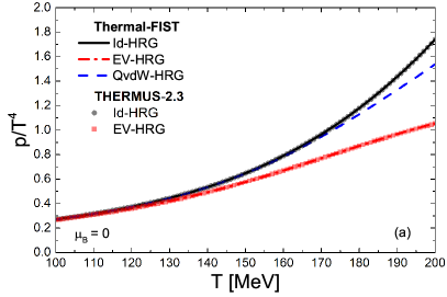
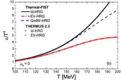
Figure 2: Temperature dependence of (a) scaled pressure $p/T^{4}$ and (b) scaled energy density $\varepsilon/T^{4}$, calculated within the Id-HRG model (solid black lines and circles), the EV-HRG model with constant radius parameter $r=0.3$ fm for all hadron species (dash-dotted red lines and squares), and the QvdW-HRG model with a vdW interaction between baryons (dashed blue lines). The lines correspond to calculations within Thermal-FIST, while the symbols depict THERMUS-2.3 calculations. Hadron list from THERMUS-2.3 is used in Thermal-FIST calculations.

The temperature dependence of the scaled pressure $p/T^{4}$ and the scaled energy density $\varepsilon/T^{4}$ calculated for the three different HRG models described above are depicted in Fig. 2 by lines (FIST) and symbols (THERMUS-2.3). One can see that the EV/vdW effects kick in at higher temperatures, where hadronic densities become large. The Thermal-FIST and THERMUS-2.3 results for Id-HRG and EV-HRG models are quantitatively consistent with each other. It is unfortunately not possible to present such a comparison for the QvdW-HRG model since THERMUS-2.3 does not contain an implementation of this model.

The annotated macro, which performs the above calculations, can be found in the following location: src/examples/cpc/cpc1-HRG-TDep.cpp

6.2 Thermal fits to heavy-ion hadron yield data

6.2.1 Excluded volume/van der Waals effects

In this subsection we consider the thermal fits to hadron yield data. It is illustrated how different EV/vdW parametrizations influence the fits. For testing purposes, we consider here those EV/vdW configurations which have a strong influence on thermal fits. In particular, we redo here some of the calculations which were presented in Ref. [45]. We take the hadron yield data measured by the ALICE collaboration in 0-5% most central Pb-Pb collisions at $\sqrt{s_{NN}}=2.76$ TeV. The actual data used in the fits can be found in Table 1 of Ref. [45]. We assume $\mu=0$, and consider the temperature dependence of $\chi^{2}$ of the fit. To calculate this temperature dependence, we minimize $\chi^{2}$ at each temperature by fitting the system volume parameter.

Four different variants of the HRG model are considered here.

1. The ideal HRG model.

2. The DEV-HRG model with mass-proportional eigenvolumes, $v_{i}=v_{p}\,(m_{i}/m_{p})$, where $v_{p}=(16/3)\pi r_{p}^{3}$ with $r_{p}=0.5$ fm is the assumed proton eigenvolume, and $m_{p}=0.938$ GeV/$c^{2}$ is the proton mass. This is the bag model HRG considered in Ref. [45].

3. The DEV-HRG model with point-like mesons, and finite-sized (anti)baryons with $v_{B}=(16/3)\pi r_{B}^{3}$, $r_{B}=0.3$ fm. This HRG model was considered in Refs. [45, 65].

4. The QvdW-HRG model which includes the QvdW interactions for baryon-baryon and antibaryon-antibaryon pairs, with QvdW parameters $a=329$ MeV fm³ and $b=3.42$ fm³, common for all pairs. This model was formulated in Ref. [29].

As in the previous example, the calculations are performed using both Thermal-FIST and THERMUS-2.3. Therefore, Thermal-FIST calculations use the hadron list from THERMUS-2.3. Quantum statistics and the energy independent Breit-Wigner modeling of finite resonance widths are used in both codes. In order to correctly calculate the feeddown contribution to the yield of the unstable $\phi$ meson, we apply the fix [86] to THERMUS-2.3.

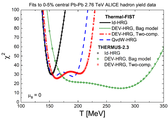
Figure 3: Temperature dependence of $\chi^{2}$ of the fits to hadron yields measured by the ALICE collaboration in 0-5% central Pb-Pb collisions at $\sqrt{s_{{}_{NN}}}=2.76$ TeV. Calculations were performed within the Id-HRG model (solid black line and circles), the DEV-HRG model with bag model parametrization of the hadron radii, with proton radius $r_{p}=0.5$ fm (dotted green line and diamonds), the DEV-HRG model with zero meson radius and $r_{B}=0.3$ fm radius for baryons (dash-dotted red line and squares), and the QvdW-HRG model (dashed blue line). The lines correspond to calculations within Thermal-FIST, while the symbols depict THERMUS-2.3 calculations. Hadron list from THERMUS-2.3 is used in Thermal-FIST calculations.

The temperature dependence of $\chi^{2}$ of the fit to the ALICE data, performed within the four models described above, is depicted in Fig. 3 by lines (Thermal-FIST) and symbols (THERMUS-2.3). The Id-HRG model shows a single $\chi^{2}$ minimum at $T\sim 155$ MeV, the result reported in the literature by many groups [34, 87, 88, 89]. Calculations within the non-ideal HRG models show peculiar two-minimum structures in Fig. 3, the mathematical origin of these structures was discussed in Refs. [45, 27]. Note that physical interpretation of the high-temperature 2nd minima should be done with care, lattice QCD calculations suggest that the crossover transition to quarks and gluons may already be completed at lower temperatures [90, 91]. The calculations are presented here merely in the context of code testing and comparison. The calculations within the Id-HRG and the two EV-HRG models are quantitatively consistent between Thermal-FIST and THERMUS-2.3. There are no THERMUS-2.3 calculations for the QvdW-HRG model available due to a lack of its implementation in THERMUS-2.3.

The annotated macro, which performs the above calculations, can be found in the following location: src/examples/cpc/cpc2-chi2-vs-T.cpp

6.2.2 Chemical non-equilibrium fits

Previous considerations were restricted to the chemical equilibrium HRG model, i.e. for $\gamma_{q}=\gamma_{S}=1$. The chemical non-equilibrium scenario, $\gamma_{q}\neq 1$, $\gamma_{S}\neq 1$, for hadron production in heavy-ion collisions was advocated in Refs. [11, 34, 92]. Fits within the chemical non-equilibrium scenario lead to significantly smaller $\chi^{2}/dof$ values. The resulting deviations from chemical equilibrium results are significant, e.g. the extracted temperature is about 15-20 MeV lower, the extracted $\gamma_{q}$ values are in the 1.6-1.7 range, very close to the Bose-Einstein condensation singularity for pions. Therefore, the improvement in fit quality comes at the cost of abandoning the chemical equilibrium scenario for heavy-ion collisions.

Here we do not discuss which physical scenario should be preferred. Instead, we verify whether the Thermal-FIST package can reproduce the previously published results obtained in the chemical non-equilibrium scenario. To our knowledge, the chemical non-equilibrium calculations were previously restricted to the usage of SHARE package.

We consider the Id-HRG model fits in Thermal-FIST within chemical equilibrium ($\gamma_{q}=\gamma_{S}=1$) and chemical non-equilibrium ($\gamma_{q}\neq 1$, $\gamma_{S}\neq 1$) scenarios. The data fitted include the 4$\pi$ multiplicities reported by the NA49 collaboration [93, 94, 95, 96, 97, 98] for most central Pb-Pb collisions at $\sqrt{s_{NN}}=7.6,\,8.8,\,12.3$, and $17.3$ GeV, and the midrapidity yields measured by the ALICE collaboration in 0-5% most central Pb-Pb collisions at $\sqrt{s_{NN}}=2.76$ TeV. These data sets are consistent with the ones analyzed with SHARE in Refs. [11, 34].

There are some technical differences between the current analysis and and previously published SHARE analyses. First, the electric charge and strangeness chemical potentials $\mu_{Q}$ and $\mu_{S}$ are not fitted here, but are fixed from the conditions of the electric-to-baryon charge ratio $Q/B=0.4$ and strangeness neutrality $S=0$. Second, there are differences in the hadron list employed in Thermal-FIST and SHARE, and there are also differences in the treatment of the finite resonance widths. Therefore, some differences between the two codes are expected, the important question is whether the qualitative features reported in Refs. [11, 34] can be reproduced.

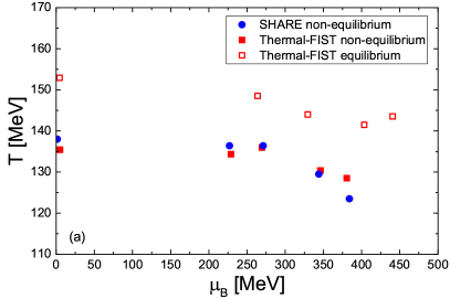
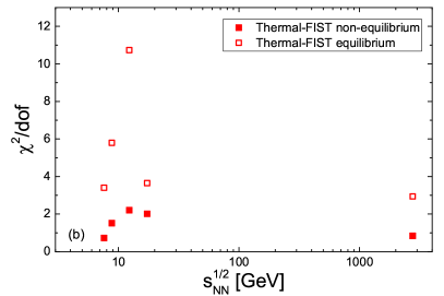
Figure 4: (a) The $T$-$\mu_{B}$ values extracted from the thermal fits to NA49 and ALICE data within the Id-HRG model in the chemical non-equilibrium (full red squares) and chemical equilibrium (open red squares) scenarios. Result of the chemical non-equilibrium fits performed within SHARE package from Refs. [11, 34] are shown by the full blue circles. (b) Energy dependence of the extracted $\chi^{2}/dof$ values from fits performed within the chemical non-equilibrium (full red squares) and chemical equilibrium (open red squares) scenarios.

The $T$-$\mu_{B}$ values extracted from the thermal fits to NA49 and ALICE data within the chemical non-equilibrium and chemical equilibrium scenarios are depicted in Fig. 4a by full and open red squares, respectively. The SHARE non-equilibrium results from Refs. [11, 34] are shown by the blue circles. The Thermal-FIST and SHARE results are consistent with each other to a good precision. The $\gamma_{q}$ values extracted from fits within Thermal-FIST are in the range $\gamma_{q}=1.6-1.7$, close to the onset of pion Bose-Einstein condensation, and consistent with the values reported in Refs. [11, 34]. Figure 4b depicts the $\chi^{2}/dof$ values obtained in chemical (non-)equilibrium fits within Thermal-FIST. The reduced $\chi^{2}$ is significantly smaller in the chemical non-equilibrium scenario, as reported in Refs. [11, 34]. The presented calculation shows that Thermal-FIST is able to reproduce previously published systematics of the chemical non-equilibrium scenario.

The annotated macro, which performs the above calculations, can be found in the following location: src/examples/cpc/cpc3-chi2NEQ.cpp

6.3 Analytic calculations vs Monte Carlo

The last section here illustrates applications of the Monte Carlo TEG. The TEG is most useful when an analytic approach is unavailable or problematic. One such example is a simultaneous inclusion of the CE and EV effects. This procedure is described in detail in Ref. [50]. Another possibility is a study of fluctuations and correlations of various hadron yields. Various effects, such as radial flow and kinematic cuts can be naturally included in the Monte Carlo approach whereas the whole procedure of the event-by-event analysis resembles closely the experimental situation.

In this section we consider a comparison of the analytic and Monte Carlo results for various 2nd order fluctuations and correlations of hadron yields. Such a comparison serves as an important cross-check of consistency between analytic and Monte Carlo methods in general, and of the probabilistic decays implementation in Sec. 2.7.2 in particular.

More specifically, we consider the mean-to-variance ratio of the net-kaon distribution $M_{k}/\sigma_{2}^{k}$, the ratio $\sigma_{11}^{Qk}/\sigma_{2}^{k}$ of the correlator between the total electric charge and final net kaon number over the variance of the final net kaon number, the ratio $\sigma_{11}^{pQ}/\sigma_{2}^{p}$ of the correlator between the final proton number and the total electric charge over the variance of the final net proton number, and the ratio $\sigma_{11}^{pk}/\sigma_{2}^{k}$ of the correlator between the final proton number and the final net kaon number over the variance of the final net kaon number, in the framework of the Id-HRG model. The beam energy dependence of $M_{k}/\sigma_{2}^{K}$ measured in Au-Au collisions was recently published by the STAR collaboration [99], while the experimental analysis of the correlation observables is ongoing.

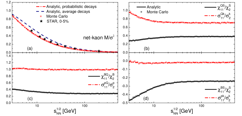
Figure 5: Collision energy dependence of (a) Net-kaon mean-to-variance ratio, (b) susceptibility ratios $\chi_{11}^{QS}/\chi_{2}^{S}$ and $\sigma_{11}^{Qk}/\sigma_{2}^{K}$, (c) $\chi_{11}^{BQ}/\chi_{2}^{B}$ and $\sigma_{11}^{pQ}/\sigma_{2}^{p}$, (d) $\chi_{11}^{BS}/\chi_{2}^{S}$ and $\sigma_{11}^{pk}/\sigma_{2}^{k}$ calculated within the Id-HRG model using analytical (lines) and Monte Carlo (symbols) methods. The stars in panel (a) depict the STAR data for net-kaon $M/\sigma^{2}$ for 0-5% central Au-Au collisions [99].

The quantities $\sigma_{2}^{k}$, $\sigma_{2}^{p}$, $\sigma_{11}^{Qk}$, $\sigma_{11}^{pQ}$, and $\sigma_{11}^{pk}$ can be expressed as linear combinations over the correlators (30) of the number of final state hadrons, which are calculated within the Thermal-FIST. The Thermal-FIST calculations here are performed along the chemical freeze-out curve of Ref. [100], the resulting beam energy dependences are shown in Fig. 5 by red lines. The red lines in Fig. 5 correspond to analytic treatment of fluctuations, including the effects of probabilistic decays.

The calculation results for the same observables using the Monte Carlo TEG are shown by the red symbols. These are consistent with the analytic results, thus verifying the accuracy of the probabilistic decay treatment implemented in Thermal-FIST. In contrast, the simplified “average” decay treatment procedure [39] leads to a markedly different result for $M_{k}/\sigma_{2}^{K}$ [dashed black curve in Fig. 5(a)] in comparison to probabilistic decays and to Monte Carlo result. Full probabilistic treatment of resonance decays thus appears to be important for interpretation of the corresponding data within the HRG approach.

The quantities $\sigma_{11}^{Qk}/\sigma_{2}^{K}$, $\sigma_{11}^{pQ}/\sigma_{2}^{p}$, and $\sigma_{11}^{pk}/\sigma_{2}^{k}$ are considered as possible proxies for the corresponding ratios of susceptiblities of conserved charges, $\chi_{11}^{QS}/\chi_{2}^{S}$, $\chi_{11}^{BQ}/\chi_{2}^{B}$, and $\chi_{11}^{BS}/\chi_{2}^{S}$. The Thermal-FIST calculations for the latter are shown in Fig. 5 by the black lines (analytical) and symbols (Monte Carlo), and these differ substantially from the measurable correlator ratios. These significant differences should be considered when interpreting the experimental data in the context of the equation of state of QCD matter.

The annotated macro, which performs the above calculations, can be found in the following location: src/examples/cpc/cpc4-mcHRG.cpp

7 Concluding remarks

The Thermal-FIST package provides the ability to perform an analysis of both, the hadronic part of the QCD equation of state and of the statistical description of hadron production in heavy-ion collisions.

The powerful graphical user interface in the package will be useful for intepreting the future hadron yield data which will come in the ongoing and future heavy-ion experiments.

Generalization and development of different variants of the HRG model is also presently an active research topic. In that regard, the flexible modular structure of Thermal-FIST is particulary suitable for continuous improvement of the package and implementation of various new features to test different new ideas.

References

References

- [1] http://eigen.tuxfamily.org
- [2] https://project-mathlibs.web.cern.ch/project-mathlibs/sw/Minuit2/html/
- [3] M. Matsumoto, T. Nishimura, Mersenne twister: a 623-dimensionally equidistributed uniform pseudo-random number generator, ACM Transactions on Modeling and Computer Simulation (TOMACS), 8 (1998) 3; Implementation by R. J. Wagner: http://www.math.sci.hiroshima-u.ac.jp/~m-mat/MT/VERSIONS/C-LANG/MersenneTwister.h
- [4] https://www.qt.io
- [5] https://www.qcustomplot.com/

References

- [1] A. Mekjian, Thermodynamic Model for Composite Particle Emission in Relativistic Heavy Ion Collisions, Phys. Rev. Lett. 38 (1977) 640–643. doi:10.1103/PhysRevLett.38.640.
- [2] J. Gosset, J. I. Kapusta, G. D. Westfall, Calculations With the Nuclear Firestreak Model, Phys. Rev. C18 (1978) 844–855. doi:10.1103/PhysRevC.18.844.
- [3] A. Z. Mekjian, Statistical Thermodynamics of Relativistic Heavy Ion Collisions, Nucl. Phys. A312 (1978) 491–523. doi:10.1016/0375-9474(78)90604-8.
- [4] H. Stoecker, A. A. Ogloblin, W. Greiner, SIGNIFICANCE OF TEMPERATURE MEASUREMENTS IN RELATIVISTIC NUCLEAR COLLISIONS, Z. Phys. A303 (1981) 259–266. doi:10.1007/BF01421522.
- [5] L. P. Csernai, J. I. Kapusta, Entropy and Cluster Production in Nuclear Collisions, Phys. Rept. 131 (1986) 223–318. doi:10.1016/0370-1573(86)90031-1.
- [6] D. Hahn, H. Stocker, Decay of instable Li, Be, and B fragments and the distortion of temperature measurements in heavy ion collisions, Phys. Rev. C35 (1987) 1311–1315. doi:10.1103/PhysRevC.35.1311.
- [7] D. Hahn, H. Stoecker, The Quantum Statistical Model of Fragment Formation: Entropy and Temperature Extraction in Heavy Ion Collisions, Nucl. Phys. A476 (1988) 718–772. doi:10.1016/0375-9474(88)90332-6.
- [8] J. Cleymans, H. Satz, Thermal hadron production in high-energy heavy ion collisions, Z. Phys. C57 (1993) 135–148. arXiv:hep-ph/9207204, doi:10.1007/BF01555746.
- [9] P. Braun-Munzinger, J. Stachel, Probing the phase boundary between hadronic matter and the quark - gluon plasma in relativistic heavy ion collisions, Nucl. Phys. A606 (1996) 320–328. arXiv:nucl-th/9606017, doi:10.1016/0375-9474(96)00198-4.
- [10] F. Becattini, J. Cleymans, A. Keranen, E. Suhonen, K. Redlich, Features of particle multiplicities and strangeness production in central heavy ion collisions between 1.7A-GeV/c and 158A-GeV/c, Phys. Rev. C64 (2001) 024901. arXiv:hep-ph/0002267, doi:10.1103/PhysRevC.64.024901.
- [11] J. Letessier, J. Rafelski, Hadron production and phase changes in relativistic heavy ion collisions, Eur. Phys. J. A35 (2008) 221–242. arXiv:nucl-th/0504028, doi:10.1140/epja/i2007-10546-7.
-
[12]
F. Becattini,
An
Introduction to the Statistical Hadronization Model, in: International
School on Quark-Gluon Plasma and Heavy Ion Collisions: past, present, future
Villa Gualino, Torino, Italy, December 8-14, 2008, 2009.
arXiv:0901.3643.
URL https://inspirehep.net/record/811687/files/arXiv:0901.3643.pdf - [13] A. Andronic, P. Braun-Munzinger, K. Redlich, J. Stachel, Decoding the phase structure of QCD via particle production at high energy, Nature 561 (7723) (2018) 321–330. arXiv:1710.09425, doi:10.1038/s41586-018-0491-6.
- [14] S. Borsanyi, Z. Fodor, S. D. Katz, S. Krieg, C. Ratti, K. Szabo, Fluctuations of conserved charges at finite temperature from lattice QCD, JHEP 01 (2012) 138. arXiv:1112.4416, doi:10.1007/JHEP01(2012)138.
- [15] A. Bazavov, et al., Fluctuations and Correlations of net baryon number, electric charge, and strangeness: A comparison of lattice QCD results with the hadron resonance gas model, Phys. Rev. D86 (2012) 034509. arXiv:1203.0784, doi:10.1103/PhysRevD.86.034509.
- [16] R. Bellwied, S. Borsanyi, Z. Fodor, S. D. Katz, A. Pasztor, C. Ratti, K. K. Szabo, Fluctuations and correlations in high temperature QCD, Phys. Rev. D92 (11) (2015) 114505. arXiv:1507.04627, doi:10.1103/PhysRevD.92.114505.
- [17] R. Bellwied, S. Borsanyi, Z. Fodor, S. D. Katz, C. Ratti, Is there a flavor hierarchy in the deconfinement transition of QCD?, Phys. Rev. Lett. 111 (2013) 202302. arXiv:1305.6297, doi:10.1103/PhysRevLett.111.202302.
- [18] G. Torrieri, S. Steinke, W. Broniowski, W. Florkowski, J. Letessier, J. Rafelski, SHARE: Statistical hadronization with resonances, Comput. Phys. Commun. 167 (2005) 229–251. arXiv:nucl-th/0404083, doi:10.1016/j.cpc.2005.01.004.
- [19] G. Torrieri, S. Jeon, J. Letessier, J. Rafelski, SHAREv2: Fluctuations and a comprehensive treatment of decay feed-down, Comput. Phys. Commun. 175 (2006) 635–649. arXiv:nucl-th/0603026, doi:10.1016/j.cpc.2006.07.010.
- [20] M. Petran, J. Letessier, J. Rafelski, G. Torrieri, SHARE with CHARM, Comput. Phys. Commun. 185 (2014) 2056–2079. arXiv:1310.5108, doi:10.1016/j.cpc.2014.02.026.
- [21] S. Wheaton, J. Cleymans, THERMUS: A Thermal model package for ROOT, Comput. Phys. Commun. 180 (2009) 84–106. arXiv:hep-ph/0407174, doi:10.1016/j.cpc.2008.08.001.
- [22] A. Kisiel, T. Taluc, W. Broniowski, W. Florkowski, THERMINATOR: THERMal heavy-IoN generATOR, Comput. Phys. Commun. 174 (2006) 669–687. arXiv:nucl-th/0504047, doi:10.1016/j.cpc.2005.11.010.
- [23] M. Chojnacki, A. Kisiel, W. Florkowski, W. Broniowski, THERMINATOR 2: THERMal heavy IoN generATOR 2, Comput. Phys. Commun. 183 (2012) 746–773. arXiv:1102.0273, doi:10.1016/j.cpc.2011.11.018.
- [24] D. H. Rischke, M. I. Gorenstein, H. Stoecker, W. Greiner, Excluded volume effect for the nuclear matter equation of state, Z. Phys. C51 (1991) 485–490. doi:10.1007/BF01548574.
- [25] G. D. Yen, M. I. Gorenstein, W. Greiner, S.-N. Yang, Excluded volume hadron gas model for particle number ratios in A+A collisions, Phys. Rev. C56 (1997) 2210–2218. arXiv:nucl-th/9711062, doi:10.1103/PhysRevC.56.2210.
- [26] G. D. Yen, M. I. Gorenstein, The Analysis of particle multiplicities in Pb + Pb collisions at CERN SPS within hadron gas models, Phys. Rev. C59 (1999) 2788–2791. arXiv:nucl-th/9808012, doi:10.1103/PhysRevC.59.2788.
- [27] L. M. Satarov, V. Vovchenko, P. Alba, M. I. Gorenstein, H. Stoecker, New scenarios for hard-core interactions in a hadron resonance gas, Phys. Rev. C95 (2) (2017) 024902. arXiv:1610.08753, doi:10.1103/PhysRevC.95.024902.
- [28] V. Vovchenko, D. V. Anchishkin, M. I. Gorenstein, Van der Waals Equation of State with Fermi Statistics for Nuclear Matter, Phys. Rev. C91 (6) (2015) 064314. arXiv:1504.01363, doi:10.1103/PhysRevC.91.064314.
- [29] V. Vovchenko, M. I. Gorenstein, H. Stoecker, van der Waals Interactions in Hadron Resonance Gas: From Nuclear Matter to Lattice QCD, Phys. Rev. Lett. 118 (18) (2017) 182301. arXiv:1609.03975, doi:10.1103/PhysRevLett.118.182301.
- [30] V. Vovchenko, A. Motornenko, P. Alba, M. I. Gorenstein, L. M. Satarov, H. Stoecker, Multicomponent van der Waals equation of state: Applications in nuclear and hadronic physics, Phys. Rev. C96 (4) (2017) 045202. arXiv:1707.09215, doi:10.1103/PhysRevC.96.045202.
- [31] P. Huovinen, P. Petreczky, Hadron Resonance Gas with Repulsive Interactions and Fluctuations of Conserved Charges, Phys. Lett. B777 (2018) 125–130. arXiv:1708.00879, doi:10.1016/j.physletb.2017.12.001.
- [32] V. Vovchenko, A. Pasztor, Z. Fodor, S. D. Katz, H. Stoecker, Repulsive baryonic interactions and lattice QCD observables at imaginary chemical potential, Phys. Lett. B775 (2017) 71–78. arXiv:1708.02852, doi:10.1016/j.physletb.2017.10.042.
- [33] V. Vovchenko, A. Motornenko, M. I. Gorenstein, H. Stoecker, Beth-Uhlenbeck approach for repulsive interactions between baryons in a hadron gas, Phys. Rev. C97 (3) (2018) 035202. arXiv:1710.00693, doi:10.1103/PhysRevC.97.035202.
- [34] M. Petrán, J. Letessier, V. Petráček, J. Rafelski, Hadron production and quark-gluon plasma hadronization in Pb-Pb collisions at TeV, Phys. Rev. C88 (3) (2013) 034907. arXiv:1303.2098, doi:10.1103/PhysRevC.88.034907.
- [35] P. Garg, D. K. Mishra, P. K. Netrakanti, B. Mohanty, A. K. Mohanty, B. K. Singh, N. Xu, Conserved number fluctuations in a hadron resonance gas model, Phys. Lett. B726 (2013) 691–696. arXiv:1304.7133, doi:10.1016/j.physletb.2013.09.019.
- [36] J. Fu, Higher moments of net-proton multiplicity distributions in heavy ion collisions at chemical freeze-out, Phys. Lett. B722 (2013) 144–150. doi:10.1016/j.physletb.2013.04.018.
- [37] P. Alba, W. Alberico, R. Bellwied, M. Bluhm, V. Mantovani Sarti, M. Nahrgang, C. Ratti, Freeze-out conditions from net-proton and net-charge fluctuations at RHIC, Phys. Lett. B738 (2014) 305–310. arXiv:1403.4903, doi:10.1016/j.physletb.2014.09.052.
- [38] P. Alba, R. Bellwied, M. Bluhm, V. Mantovani Sarti, M. Nahrgang, C. Ratti, Sensitivity of multiplicity fluctuations to freeze-out conditions in heavy ion collisions, Phys. Rev. C92 (6) (2015) 064910. arXiv:1504.03262, doi:10.1103/PhysRevC.92.064910.
- [39] M. Nahrgang, M. Bluhm, P. Alba, R. Bellwied, C. Ratti, Impact of resonance regeneration and decay on the net-proton fluctuations in a hadron resonance gas, Eur. Phys. J. C75 (12) (2015) 573. arXiv:1402.1238, doi:10.1140/epjc/s10052-015-3775-0.
- [40] V. Vovchenko, V. V. Begun, M. I. Gorenstein, Hadron multiplicities and chemical freeze-out conditions in proton-proton and nucleus-nucleus collisions, Phys. Rev. C93 (6) (2016) 064906. arXiv:1512.08025, doi:10.1103/PhysRevC.93.064906.
- [41] V. V. Begun, V. Vovchenko, M. I. Gorenstein, H. Stoecker, Statistical hadron-gas treatment of systems created in proton-proton interactions at CERN SPS, Phys. Rev. C98 (5) (2018) 054909. arXiv:1805.01901, doi:10.1103/PhysRevC.98.054909.
- [42] V. Begun, D. Kikoła, V. Vovchenko, D. Wielanek, Estimation of the freeze-out parameters reachable in a fixed-target experiment at the CERN Large Hadron Collider, Phys. Rev. C98 (3) (2018) 034905. arXiv:1806.01303, doi:10.1103/PhysRevC.98.034905.
- [43] V. Vovchenko, M. I. Gorenstein, H. Stoecker, Finite resonance widths influence the thermal-model description of hadron yields, Phys. Rev. C98 (3) (2018) 034906. arXiv:1807.02079, doi:10.1103/PhysRevC.98.034906.
- [44] A. Motornenko, V. V. Begun, V. Vovchenko, M. I. Gorenstein, H. Stoecker, Hadron yields and fluctuations at energies available at the CERN Super Proton Synchrotron: System-size dependence from Pb + Pb to + collisions, Phys. Rev. C99 (3) (2019) 034909. arXiv:1811.10645, doi:10.1103/PhysRevC.99.034909.
- [45] V. Vovchenko, H. Stöcker, Surprisingly large uncertainties in temperature extraction from thermal fits to hadron yield data at LHC, J. Phys. G44 (5) (2017) 055103. arXiv:1512.08046, doi:10.1088/1361-6471/aa6409.
- [46] V. Vovchenko, H. Stoecker, Examination of the sensitivity of the thermal fits to heavy-ion hadron yield data to the modeling of the eigenvolume interactions, Phys. Rev. C95 (4) (2017) 044904. arXiv:1606.06218, doi:10.1103/PhysRevC.95.044904.
- [47] P. Alba, V. Vovchenko, M. I. Gorenstein, H. Stoecker, Flavor-dependent eigenvolume interactions in a hadron resonance gas, Nucl. Phys. A974 (2018) 22–34. arXiv:1606.06542, doi:10.1016/j.nuclphysa.2018.03.007.
- [48] D. Anchishkin, V. Vovchenko, Mean-field approach in the multi-component gas of interacting particles applied to relativistic heavy-ion collisions, J. Phys. G42 (10) (2015) 105102. arXiv:1411.1444, doi:10.1088/0954-3899/42/10/105102.
- [49] V. Vovchenko, D. V. Anchishkin, M. I. Gorenstein, Hadron Resonance Gas Equation of State from Lattice QCD, Phys. Rev. C91 (2) (2015) 024905. arXiv:1412.5478, doi:10.1103/PhysRevC.91.024905.
- [50] V. Vovchenko, M. I. Gorenstein, H. Stoecker, Monte Carlo approach to the excluded-volume hadron resonance gas in grand canonical and canonical ensembles, Phys. Rev. C98 (6) (2018) 064909. arXiv:1805.01402, doi:10.1103/PhysRevC.98.064909.
- [51] V. Vovchenko, Equations of state for real gases on the nuclear scale, Phys. Rev. C96 (1) (2017) 015206. arXiv:1701.06524, doi:10.1103/PhysRevC.96.015206.
- [52] V. Vovchenko, M. I. Gorenstein, H. Stoecker, Modeling baryonic interactions with the Clausius-type equation of state, Eur. Phys. J. A54 (2) (2018) 16. arXiv:1709.10097, doi:10.1140/epja/i2018-12399-3.
- [53] V. Vovchenko, L. Jiang, M. I. Gorenstein, H. Stoecker, Critical point of nuclear matter and beam energy dependence of net proton number fluctuations, Phys. Rev. C98 (2) (2018) 024910. arXiv:1711.07260, doi:10.1103/PhysRevC.98.024910.
- [54] V. Vovchenko, H. Stoecker, Analysis of hadron yield data within hadron resonance gas model with multi-component eigenvolume corrections, J. Phys. Conf. Ser. 779 (1) (2017) 012078. arXiv:1610.02346, doi:10.1088/1742-6596/779/1/012078.
- [55] V. Vovchenko, B. Dönigus, H. Stoecker, Multiplicity dependence of light nuclei production at LHC energies in the canonical statistical model, Phys. Lett. B785 (2018) 171–174. arXiv:1808.05245, doi:10.1016/j.physletb.2018.08.041.
- [56] J. Letessier, J. Rafelski, Chemical nonequilibrium and deconfinement in 200-A/GeV sulphur induced reactions, Phys. Rev. C59 (1999) 947–954. arXiv:hep-ph/9806386, doi:10.1103/PhysRevC.59.947.
- [57] P. Koch, B. Muller, J. Rafelski, Strangeness in Relativistic Heavy Ion Collisions, Phys. Rept. 142 (1986) 167–262. doi:10.1016/0370-1573(86)90096-7.
- [58] J. Rafelski, Strange anti-baryons from quark - gluon plasma, Phys. Lett. B262 (1991) 333–340. doi:10.1016/0370-2693(91)91576-H.
- [59] J. Baacke, Thermodynamics of a Gas of MIT Bags, Acta Phys. Polon. B8 (1977) 625.
- [60] R. Hagedorn, J. Rafelski, Hot Hadronic Matter and Nuclear Collisions, Phys. Lett. 97B (1980) 136. doi:10.1016/0370-2693(80)90566-3.
- [61] R. Hagedorn, The Pressure Ensemble as a Tool for Describing the Hadron - Quark Phase Transition, Z. Phys. C17 (1983) 265. doi:10.1007/BF01578153.
- [62] M. I. Gorenstein, V. K. Petrov, G. M. Zinovev, Phase Transition in the Hadron Gas Model, Phys. Lett. 106B (1981) 327–330. doi:10.1016/0370-2693(81)90546-3.
- [63] J. I. Kapusta, K. A. Olive, Thermodynamics of Hadrons: Delimiting the Temperature, Nucl. Phys. A408 (1983) 478–494. doi:10.1016/0375-9474(83)90241-5.
- [64] P. Braun-Munzinger, I. Heppe, J. Stachel, Chemical equilibration in Pb + Pb collisions at the SPS, Phys. Lett. B465 (1999) 15–20. arXiv:nucl-th/9903010, doi:10.1016/S0370-2693(99)01076-X.
- [65] A. Andronic, P. Braun-Munzinger, J. Stachel, M. Winn, Interacting hadron resonance gas meets lattice QCD, Phys. Lett. B718 (2012) 80–85. arXiv:1201.0693, doi:10.1016/j.physletb.2012.10.001.
- [66] M. I. Gorenstein, A. P. Kostyuk, Ya. D. Krivenko, Van der Waals excluded volume model of multicomponent hadron gas, J. Phys. G25 (1999) L75–L83. arXiv:nucl-th/9906068, doi:10.1088/0954-3899/25/9/102.
- [67] C. G. Broyden, A class of methods for solving nonlinear simultaneous equations, Mathematics of Computation 19 (92) (1965) 577.
- [68] K. Fukushima, Hadron resonance gas and mean-field nuclear matter for baryon number fluctuations, Phys. Rev. C91 (4) (2015) 044910. arXiv:1409.0698, doi:10.1103/PhysRevC.91.044910.
- [69] A. Mukherjee, J. Steinheimer, S. Schramm, Higher-order baryon number susceptibilities: interplay between the chiral and the nuclear liquid-gas transitions, Phys. Rev. C96 (2) (2017) 025205. arXiv:1611.10144, doi:10.1103/PhysRevC.96.025205.
- [70] F. Becattini, A Thermodynamical approach to hadron production in e+ e- collisions, Z. Phys. C69 (3) (1996) 485–492. doi:10.1007/BF02907431.
- [71] S. Jeon, V. Koch, Charged particle ratio fluctuation as a signal for QGP, Phys. Rev. Lett. 85 (2000) 2076–2079. arXiv:hep-ph/0003168, doi:10.1103/PhysRevLett.85.2076.
- [72] V. V. Begun, M. I. Gorenstein, M. Hauer, V. P. Konchakovski, O. S. Zozulya, Multiplicity Fluctuations in Hadron-Resonance Gas, Phys. Rev. C74 (2006) 044903. arXiv:nucl-th/0606036, doi:10.1103/PhysRevC.74.044903.
- [73] M. I. Gorenstein, M. Hauer, D. O. Nikolajenko, Particle number fluctuations in nuclear collisions within excluded volume hadron gas model, Phys. Rev. C76 (2007) 024901. arXiv:nucl-th/0702081, doi:10.1103/PhysRevC.76.024901.
- [74] F. Becattini, U. W. Heinz, Thermal hadron production in p p and p anti-p collisions, Z. Phys. C76 (1997) 269–286, [Erratum: Z. Phys.C76,578(1997)]. arXiv:hep-ph/9702274, doi:10.1007/s002880050551.
- [75] A. Keranen, F. Becattini, Chemical factors in canonical statistical models for relativistic heavy ion collisions, Phys. Rev. C65 (2002) 044901, [Erratum: Phys. Rev.C68,059901(2003)]. arXiv:nucl-th/0112021, doi:10.1103/PhysRevC.65.044901,10.1103/PhysRevC.68.059901.
- [76] P. Braun-Munzinger, J. Cleymans, H. Oeschler, K. Redlich, Maximum relative strangeness content in heavy ion collisions around 30-GeV/A, Nucl. Phys. A697 (2002) 902–912. arXiv:hep-ph/0106066, doi:10.1016/S0375-9474(01)01257-X.
- [77] F. James, M. Roos, Minuit: A System for Function Minimization and Analysis of the Parameter Errors and Correlations, Comput. Phys. Commun. 10 (1975) 343–367. doi:10.1016/0010-4655(75)90039-9.
- [78] J. Rafelski, Melting Hadrons, Boiling Quarks, Eur. Phys. J. A51 (9) (2015) 114. arXiv:1508.03260, doi:10.1140/epja/i2015-15114-0.
- [79] F. Becattini, L. Ferroni, Statistical hadronization and hadronic microcanonical ensemble. 2., Eur. Phys. J. C38 (2004) 225–246, [Erratum: Eur. Phys. J.66,341(2010)]. arXiv:hep-ph/0407117, doi:10.1140/epjc/s10052-010-1243-4,10.1140/epjc/s2004-02027-8.
- [80] P. J. Siemens, J. O. Rasmussen, Evidence for a blast wave from compress nuclear matter, Phys. Rev. Lett. 42 (1979) 880–887. doi:10.1103/PhysRevLett.42.880.
- [81] E. Schnedermann, J. Sollfrank, U. W. Heinz, Thermal phenomenology of hadrons from 200-A/GeV S+S collisions, Phys. Rev. C48 (1993) 2462–2475. arXiv:nucl-th/9307020, doi:10.1103/PhysRevC.48.2462.
-
[82]
Thermal-FIST documentation, [Online; accessed 25-June-2019].
URL https://fias.uni-frankfurt.de/~vovchenko/project/thermal-fist/doc/ - [83] L. Landau, E. Lifshitz, Fluid Mechanics, Pergamon Press, 1987.
- [84] L. M. Satarov, M. N. Dmitriev, I. N. Mishustin, Equation of state of hadron resonance gas and the phase diagram of strongly interacting matter, Phys. Atom. Nucl. 72 (2009) 1390–1415. arXiv:0901.1430, doi:10.1134/S1063778809080146.
-
[85]
The Qt Company, Qt framework, [Online; accessed
5-November-2018].
URL https://www.qt.io/ -
[86]
V. Vovchenko, The
THERMUS decays fix, [Online; accessed 25-June-2019].
URL https://github.com/vlvovch/thermus-decays-fix - [87] J. Stachel, A. Andronic, P. Braun-Munzinger, K. Redlich, Confronting LHC data with the statistical hadronization model, J. Phys. Conf. Ser. 509 (2014) 012019. arXiv:1311.4662, doi:10.1088/1742-6596/509/1/012019.
- [88] M. Floris, Hadron yields and the phase diagram of strongly interacting matter, Nucl. Phys. A931 (2014) 103–112. arXiv:1408.6403, doi:10.1016/j.nuclphysa.2014.09.002.
- [89] F. Becattini, E. Grossi, M. Bleicher, J. Steinheimer, R. Stock, Centrality dependence of hadronization and chemical freeze-out conditions in heavy ion collisions at = 2.76 TeV, Phys. Rev. C90 (5) (2014) 054907. arXiv:1405.0710, doi:10.1103/PhysRevC.90.054907.
- [90] S. Borsanyi, Z. Fodor, C. Hoelbling, S. D. Katz, S. Krieg, C. Ratti, K. K. Szabo, Is there still any mystery in lattice QCD? Results with physical masses in the continuum limit III, JHEP 09 (2010) 073. arXiv:1005.3508, doi:10.1007/JHEP09(2010)073.
- [91] A. Bazavov, et al., The chiral and deconfinement aspects of the QCD transition, Phys. Rev. D85 (2012) 054503. arXiv:1111.1710, doi:10.1103/PhysRevD.85.054503.
- [92] M. Petran, J. Rafelski, Universal hadronization condition in heavy ion collisions at GeV and at TeV, Phys. Rev. C88 (2) (2013) 021901. arXiv:1303.0913, doi:10.1103/PhysRevC.88.021901.
- [93] S. V. Afanasiev, et al., Energy dependence of pion and kaon production in central Pb + Pb collisions, Phys. Rev. C66 (2002) 054902. arXiv:nucl-ex/0205002, doi:10.1103/PhysRevC.66.054902.
- [94] C. Alt, et al., Energy and centrality dependence of anti-p and p production and the anti-Lambda/anti-p ratio in Pb+Pb collisions between 20/A-GeV and 158/A-Gev, Phys. Rev. C73 (2006) 044910. doi:10.1103/PhysRevC.73.044910.
- [95] C. Alt, et al., Pion and kaon production in central Pb + Pb collisions at 20-A and 30-A-GeV: Evidence for the onset of deconfinement, Phys. Rev. C77 (2008) 024903. arXiv:0710.0118, doi:10.1103/PhysRevC.77.024903.
- [96] C. Alt, et al., Energy dependence of Lambda and Xi production in central Pb+Pb collisions at A-20, A-30, A-40, A-80, and A-158 GeV measured at the CERN Super Proton Synchrotron, Phys. Rev. C78 (2008) 034918. arXiv:0804.3770, doi:10.1103/PhysRevC.78.034918.
- [97] C. Alt, et al., Energy dependence of phi meson production in central Pb+Pb collisions at s(NN)**(1/2) = 6 to 17 GeV, Phys. Rev. C78 (2008) 044907. arXiv:0806.1937, doi:10.1103/PhysRevC.78.044907.
- [98] C. Alt, et al., Omega- and anti-Omega+ production in central Pb + Pb collisions at 40-AGeV and 158-AGeV, Phys. Rev. Lett. 94 (2005) 192301. arXiv:nucl-ex/0409004, doi:10.1103/PhysRevLett.94.192301.
- [99] L. Adamczyk, et al., Collision Energy Dependence of Moments of Net-Kaon Multiplicity Distributions at RHIC, Phys. Lett. B785 (2018) 551–560. arXiv:1709.00773, doi:10.1016/j.physletb.2018.07.066.
- [100] J. Cleymans, H. Oeschler, K. Redlich, S. Wheaton, Comparison of chemical freeze-out criteria in heavy-ion collisions, Phys. Rev. C73 (2006) 034905. arXiv:hep-ph/0511094, doi:10.1103/PhysRevC.73.034905.