The Discrete Langevin Machine:
Bridging the Gap Between Thermodynamic and Neuromorphic Systems

Abstract

A formulation of Langevin dynamics for discrete systems is derived as a class of generic stochastic processes. The dynamics simplify for a two-state system and suggest a network architecture which is implemented by the Langevin machine. The Langevin machine represents a promising approach to compute successfully quantitative exact results of Boltzmann distributed systems by LIF neurons. Besides a detailed introduction of the dynamics, different simplified models of a neuromorphic hardware system are studied with respect to a control of emerging sources of errors.

I Introduction

The rapidly increasing progress on neuromorphic computing and the ongoing research of spiking systems as the third generation of neural networks calls for a better understanding of fundamental processes of neuromorphic hardware systems [1, 2, 3, 4, 5, 6]; for a recent review on neuromorphic computing see [7]. As a parallel computing platform, these systems may be used in the long run to accurately simulate and compute large systems, in particular given their low energy consumption.

Possible applications range from an effective implementation of artificial neural networks and further machine learning methods [8, 9, 10, 11, 12, 13] over a better understanding of biological processes in our brains [14, 15] to the computation of physical and stochastic interesting systems [16, 17, 18]. Many artificial neural networks and physical systems are described by Boltzmann distributed systems. For a quantitatively accurate computation of such systems, it is necessary to deduce an exact representation on neuromorphic hardware systems [19, 11, 20, 21], in particular for systematic error estimates.

Our work is motivated by the similarity of Langevin dynamics and leaky integrate-and-fire (LIF) neurons for performing stochastic inference [22]. Indeed, the fundamental dynamics of LIF neurons is governed by Langevin dynamics. Apart from its obvious relevance for the description of stochastical processes, the Langevin equation [23] can also be used for simulating quantum field theories with stochastic quantization [24, 25, 26]. In this approach the Euclidean path integral measure is obtained as the stationary distribution of a stochastic process. This paves the way to the heuristic approach of using complex Langevin dynamics as a potential method for accessing real time dynamics and sign problems. The latter problem is, e.g. prominent in QCD at finite chemical potential [27, 28, 29]. A further interesting application of the Langevin equation can be found in [30]. Langevin dynamics is combined with a stochastic gradient descent algorithm to perform Bayesian learning which enables an uncertainty estimation of resulting parameters.

Many of the above mentioned systems are discrete ones, the simplest one being a two-state system. This suggests the formulation of a discrete analog to continuous Langevin dynamics, for the accurate description of discrete systems. In the present work, we show that a formulation of Langevin dynamics for discrete systems leads to a class of a generic stochastic process, namely, the Langevin equation for discrete systems,

$$\phi^{\prime}=\phi+(\nu-\phi)\Theta\left[-1-\frac{\epsilon}{2\lambda_{\epsilon}}\Delta S(\nu,\phi)+\sqrt{\epsilon}\tilde{\eta}\right]\,,$$ (1)

where $\phi$ is the current state and $\phi^{\prime}$ the updated state. The process is driven by a Gaussian noise term $\tilde{\eta}$. The parameter $\epsilon$ has an impact on the acceptance probability of the proposed state $\nu$ and should be chosen small. The term $\Delta S(\nu,\phi):=S(\nu)-S(\phi)$ measures the change of the action $S$ of the system under a transition from state $\phi$ to the proposed state $\nu$. A more detailed derivation of (1) including a discussion of its properties can be found in Section III. The dynamics leads in the limit of $\epsilon\to 0$ to Boltzmann distributed states.

The present work concentrates on the potential of the process for a more accurate implementation of Boltzmann distributed systems on the neuromorphic hardware. This leads to an architecture of neurons based on a self-interacting contribution. The self-interacting term changes manifestly the dynamics of the neural network. This results in an activation function which is much closer to a logistic distribution, the activation function of a Boltzmann machine, than existing approaches. The architecture can be applied to both, discrete two-state systems and neuromorphic hardware systems with a continuous membrane potential and a spiking character. The dynamics differ in their kind of noise that is uncorrelated in the former case and autocorrelated in the latter case. In this work spiking character refers to an effective mapping of a continuous potential to two discrete neuron states in an interacting system. Figure 1 compares the different network structures and gives an overview over existing and contributed dynamics of this work.

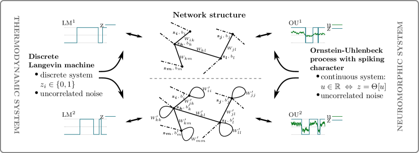
Figure 1: Comparison of the commonly used network structure (upper row) and the presented architecture with a self-interacting contribution (lower row). Both network structures can be considered as systems of two discrete states with an uncorrelated noise contribution, which corresponds to different implementations of the discrete Langevin machine. Their continuous counterpart is represented by an Ornstein-Uhlenbeck process with spiking character. The dynamics is based on the temporal evolution of a membrane potential $u:=u_{\textnormal{eff}}(t)$. The interaction of neurons relies on a projection of the potential onto two states and enables a comparison with the Langevin machine. The processes on the right-hand side are already very close to the fundamental dynamics of LIF sampling.

An exact representation of the activation function of the Boltzmann machine is necessary to obtain correct statistics in coupled systems on neuromorphic hardware systems. In the present work we show in a detailed numerical analysis that small deviations in the activation function propagate if a rectangular refractory mechanism or interactions between neurons are taken into account. These small deviations have a large impact on the resulting correlation functions and observables. The numerical results demonstrate that a reliable estimation, an understanding and a control of different sources of errors are essential for a correct computation of Boltzmann distributed systems in the future.

An introduction to Langevin dynamics is given in Section II. The Langevin equation for discrete systems is derived in Section III. In Section IV, the so-called sign-dependent discrete Langevin machine is introduced as a special case of the Langevin equation for discrete systems. The mapping of different dynamics of discrete systems onto an Ornstein-Uhlenbeck process with spiking character is discussed in Section V. Section VI recapitulates relations between the discrete Langevin machine and the neuromorphic hardware. In Section VII, numerical results of the introduced and of existing dynamics are presented, possible sources of errors are extracted and the propagation of errors for different abstractions of a neuromorphic hardware system is analyzed. The conclusion and outlook can be found in Section VIII.

II Metropolis Algorithm Versus Langevin Dynamics

The section reviews shortly properties of the Metropolis algorithm [31] and Langevin dynamics for continuous systems to get a first intuition on how a possible Langevin equation for a discrete system could look like. The considerations are inspired by the work in [32, 33, 34].

II.1 Langevin dynamics

We adopt the common formulation of the Langevin equation within the study of Euclidean quantum field theories [24, 25],

$$\frac{\partial}{\partial\tau}\phi_{x}(\tau)=-\frac{\delta S_{E}}{\delta\phi_{x}(\tau)}+\eta_{x}(\tau)\,,$$ (2)

where $S_{E}$ corresponds to the Euclidean action, which depends on fields $\phi_{x}(\tau)$ on a (3+1)-dimensional hypercubic lattice in Euclidean space. The Langevin equation describes the evolution of the quantum fields $\phi_{x}(\tau)$ in an additional fictious time dimension, the Langevin time $\tau$. Quantum fluctuations are emulated by the additional white Gaussian noise term with the properties to be uncorrelated,

$$\langle\eta_{i},\eta^{\prime}_{j}\rangle_{\eta}=2\delta(j-i)\delta(t^{\prime}-t)\,,\quad\langle\eta_{i}\rangle_{\eta}=0\,.$$ (3)

It can be shown that in equilibrium the resulting distribution of the fields coincides with the Boltzmann distribution: $\lim\limits_{\tau\to\infty}P(\phi,t)=P_{\textnormal{eq}}(\phi)=\frac{1}{Z}\exp(-S_{E})$. A common approach to prove this is to derive the equivalence of the Langevin equation and the Fokker-Planck equation in a first step and to compute the static solution in a second step [24]. This property renders Langevin dynamics a powerful tool in QCD [27, 28] and beyond.

II.2 Equivalence to a Monte Carlo algorithm

The transition probability $W(\phi\to\phi^{\prime})$ for Langevin dynamics is derived in Appendix A. It is computed based on a discrete form of the Langevin equation where an infinitesimal update step of a field $\phi:=\phi(\tau)$ to a field $\phi^{\prime}:=\phi(\tau+\epsilon)$ is considered. The resulting transition probability can be rewritten as

$$W(\phi\to\phi^{\prime})=\frac{1}{\sqrt{2\epsilon}}\varphi\left(\frac{\phi^{\prime}-\phi}{\sqrt{2\epsilon}}\right)\exp\left[-\frac{S(\phi^{\prime})-S(\phi)}{2}\right]\,.$$ (4)

The first factor can be interpreted as the selection probability of a field and the second term as the acceptance probability. There are two adaptations to the Metropolis algorithm [31]. First, the acceptance probability has the additional factor of $2$. This factor is necessary to satisfy the detailed balance equation. Second, the proposal state is chosen to be an infinitesimal change to the current state. This ensures a correct normalization of the transition probability for $\epsilon\to 0$, as can be seen by replacing the selection probability by the delta distribution,

$$\int_{-\infty}^{\infty} d\phi^{\prime}W(\phi\to\phi^{\prime})=$$

$$=\int_{-\infty}^{\infty}d\phi^{\prime}\delta(\phi^{\prime}-\phi)\exp\left[-\frac{S(\phi^{\prime})-S(\phi)}{2}\right]=1\,.$$ (5)

The update mechanism of Langevin dynamics can be parallelized because of these two properties.

Accordingly, the Langevin equation (2) can be interpreted as a standard Monte Carlo algorithm with a Gaussian distribution as selection probability. The proposal state is chosen implicitly by an absorption of the acceptance probability into the selection probability and by a corresponding sampling with Gaussian noise. Since the nearest neighbor sites can be assumed to be nearly constant in one Monte Carlo step, it is possible to switch from a random sequential update formalism to a parallel update of the entire lattice. The Langevin time is introduced as a temporal measure for a lattice update. In principle, the delta distribution can be exchanged by any other positive representation. In some cases one can derive Langevin dynamics with another noise source by an equivalent approximation (for example, Cauchy noise).

Having the knowledge of this section, a Langevin equation for discrete systems can be constructed by considering a standard Monte Carlo algorithm.

III Discrete Langevin Dynamics

The formulation of the Langevin equation for discrete systems is derived inspired by the comparison of the Metropolis algorithm and Langevin dynamics in the previous section. The general formulation of a Langevin equation for discrete systems presented in this section is similar to a Monte Carlo algorithm and is driven by a Gaussian noise contribution. The transition probability to a proposed state is regulated by the introduction of truncating Gaussian noise. It is shown that the accuracy of the process strongly depends on an intrinsic parameter $\epsilon$ and the scale of the energy contribution.

Certain necessary properties of a possible Langevin equation for discrete systems can be stated beforehand based on the comparison of Langevin dynamics and the Metropolis algorithm in Section II. First, an infinitesimal change of the microscopic state/field is not possible. Therefore, one has to switch from a parallel to a random sequential update mechanism. Further, the computer time is the timescale of the approach. The proposal field has to be chosen from a discrete distribution. One may select the proposal field according to some distribution around the current field. However, since a parallelization is not possible, the uniform selection probability of a Metropolis algorithm can be adopted.

Assuming the same acceptance probability as in the continuous case, a starting point is the following proportionality:

$$W(\phi\to\phi^{\prime})\propto\exp\left[-\frac{S(\phi^{\prime})-S(\phi)}{2}\right]\,.$$ (6)

With the help of a relation between the cumulative Gaussian distribution $\Phi(x)$ and the exponential function, given by (54), and with $\Delta S(\phi^{\prime},\phi)=S(\phi^{\prime})-S(\phi)$, this can be rewritten in the following way:

$$W(\phi\to\phi^{\prime}) \propto\Phi\left(-\frac{1}{\sqrt{\epsilon}}-\frac{\sqrt{\epsilon}}{2\lambda_{\epsilon}}\Delta S(\phi^{\prime},\phi)\right)=$$

$$=P\left(\tilde{\eta}<-\frac{1}{\sqrt{\epsilon}}-\frac{\sqrt{\epsilon}}{2\lambda_{\epsilon}}\Delta S(\phi^{\prime},\phi)\right)\,,$$ (7)

for $\epsilon\to 0$. An analytical expression for the additional scaling factor $\lambda_{\epsilon}$ is given in equation (55).

The Gaussian noise contribution $\tilde{\eta}$ is uncorrelated and has variance $1$,

$$\langle\tilde{\eta}_{i},\tilde{\eta}^{\prime}_{j}\rangle_{\tilde{\eta}}=\delta(j-i)\delta(t^{\prime}-t)\,,\qquad\langle\tilde{\eta}_{i}\rangle_{\tilde{\eta}}=0\,.$$ (8)

Taking the current state $\phi$ into account, one can transform the sampling from the cumulative normal distribution into a general stochastic update rule with Gaussian noise and a proposal state $\nu$. This leads us to (1), which was already presented in the introduction,

$$\phi^{\prime}=\phi+(\nu-\phi)\Theta\left[-1-\frac{\epsilon}{2\lambda_{\epsilon}}\Delta S(\nu,\phi)+\sqrt{\epsilon}\tilde{\eta}\right]\,,$$ (9)

where $\epsilon$ needs to be chosen sufficiently small. $\Theta(x)$ represents the Heaviside function.

The update formalism corresponds to a single spin flip Monte Carlo algorithm with a random sequential update mechanism, driven by Gaussian noise. It can be immediately seen within the present form that a flip to a proposed field gets the more unlikely the smaller $\epsilon$. Adaptations of the Gaussian noise term to truncated Gaussian noise can help to improve the dynamics, i.e., to increase the probability of a spin flip. In principle, this corresponds to a rescaling of the transition probability term similar to a maximization of the spin flip probability in the Metropolis algorithm.

The truncated Gaussian noise term can be expressed by the following parametrization:

$$\tilde{\eta}^{T}\in\left[\frac{1}{\sqrt{\epsilon}}+\alpha,\infty\right]\,,$$ (10)

where $\alpha$ is in the range of

$$-\infty\leq\alpha\leq-\frac{\sqrt{\epsilon}}{2\lambda_{\epsilon}}\Delta_{\max}\,,\quad\textnormal{with}\quad\Delta_{\max}=|\Delta S(\nu,\phi)|\,.$$ (11)

The improved update rule is

$$\phi^{\prime}=\phi+(\nu-\phi)\Theta\left[-1-\frac{\epsilon}{2\lambda_{\epsilon}}\Delta S(\nu,\phi)+\sqrt{\epsilon}\tilde{\eta}^{T}\right]\,.$$ (12)

For $\alpha\to-\infty$ this reduces to the update formalism (9) and for $\alpha=-\frac{\sqrt{\epsilon}}{2\lambda_{\epsilon}}\Delta_{\max}$ one obtains spin flip probabilities up to $1$. This can be seen under consideration of the explicit transition probability of the update rule (12),

$$W(\phi\to\nu)=\frac{\Phi\left(-\frac{1}{\sqrt{\epsilon}}-\frac{\sqrt{\epsilon}}{2\lambda_{\epsilon}}\Delta S(\nu,\phi)\right)}{\Phi\left(-\frac{1}{\sqrt{\epsilon}}-\alpha\right)}\,.$$ (13)

Transition probabilities of further standard Monte Carlo algorithms can be emulated by other choices of $\alpha$. Note that for a uniform random number $r\in[0,1[$ and a proposal field $\nu$, an equivalent formulation to (12) can be stated for the transition probability (6),

$$\phi^{\prime}=\phi+(\nu-\phi)\Theta\left[\exp\left(-\frac{S(\nu)-S(\phi)+\Delta_{\max}}{2}\right)-r\right]\,.$$ (14)

Processes with a different value of $\alpha$, i.e., a different rescaling of the transition probability, can always be mapped onto each other by a respective rescaling of the time. Given a transition probability $W(\phi\to\mu)$ and a scaling factor $a$, the following relation holds:

$$W(\phi\to\mu)\to aW(\phi\to\mu)\quad\Leftrightarrow\quad t\to\frac{t}{a}\,.$$ (15)

Most of the existing single spin flip algorithms can be reformulated into a Langevin equation for discrete systems with the same derivation, as presented in this section. However, it can be shown that for the particular choice of the transition probability according to equation (6), the resulting order of accuracy in the detailed balance equation is the best one, with $\mathcal{O}\left(\epsilon\Delta S(\nu,\phi)^{3}\right)$. In general, it holds for the presented dynamics that

$$\lim\limits_{\epsilon\to 0}P_{\textnormal{eq}}(\phi)\propto\exp\left[-S(\phi)\right]\,.$$ (16)

The update formalism (12) represents a Langevin-like equivalent for discrete systems to Langevin dynamics of continuous systems. As for continuous systems, the dynamics depends on Gaussian noise and is based on a rather simple expression. The algorithms can also be applied to continuous systems due to the equivalence to standard Monte Carlo algorithms in the limit $\epsilon\to 0$.

IV Sign-Dependent Discrete Langevin Machine

The Langevin equation for discrete systems (12) turns into a rather simple expression for a two-state system. The resulting dynamics is introduced in the following as sign-dependent discrete Langevin machine ($\textnormal{LM}^{2}$). The $\textnormal{LM}^{2}$ represents a architecture for interacting neurons with the particularity of a self-interacting contribution. The derived network structure results in a basic dynamics with different weights and biases compared to the Boltzmann machine. It has the unique property that the equilibrium distribution converges in the limit $\epsilon\to 0$, despite a different underlying dynamics, to a logistic distribution, the activation function of the Boltzmann machine.

We define the energy of the Boltzmann machine in the common way by

$$E=-\sum_{i<j}W_{ij}z_{i}z_{j}-\sum_{i}b_{i}z_{i}\,,$$ (17)

where $W_{ij}$ are symmetric weights between the neurons $i$ and $j$ and $b_{i}$ is some additional bias. The domain of definition of the states $z_{i}$ at each neuron is given by $z_{i}\in\{0,1\}$.

Figure 2: Comparison of the structure of a Boltzmann machine (a) and that of the sign-dependent discrete Langevin machine (b). The $\textnormal{LM}^{2}$ has a self-interacting term and rescaled weights and biases. Nevertheless the dynamics leads in equilibrium to a Boltzmann distribution.

For applying the generalized update rule (12) we need the following identifications: $S\to E$ and $\phi_{i}\to z_{i}$. As discussed in Appendix E, the following simplified update rule can be derived for the $\textnormal{LM}^{2}$:

$$z^{\prime}_{i}=\Theta\left[W^{\prime}_{ii}z_{i}+\sum_{j}W^{\prime}_{ij}z_{j}+b^{\prime}_{i}+\tilde{\eta}^{T}\right]\,,$$ (18)

where the transformed parameters are defined as follows: $W^{\prime}_{ii}=\frac{2}{\sqrt{\epsilon}}$, $W^{\prime}_{ij}=\frac{\sqrt{\epsilon}}{2\lambda_{\epsilon}}W_{ij}$, and $b^{\prime}_{i}=\left(\frac{\sqrt{\epsilon}}{2\lambda_{\epsilon}}b_{i}-\frac{1}{\sqrt{\epsilon}}\right)$. Figure 2 illustrates a comparison between the structure of the Boltzmann machine and the update dynamics. The activation function of the $\textnormal{LM}^{2}$ is given in the limit of $\epsilon\to 0$ by a logistic distribution,

$$\lim\limits_{\epsilon\to 0}P_{\textnormal{LM}^{2}}(z_{i}=1)=\frac{1}{1+\exp\left[-\sum_{j}W_{ij}z_{j}-b_{i}\right]}\,.$$ (19)

The term Langevin machine is chosen because of the similarity of the network to the Boltzmann machine and to Langevin dynamics. The adjective discrete is added to avoid confusion with the Langevin machine presented in [35]. The noise term in the dynamics can be chosen according to equation (10), i.e., it can be a Gaussian noise or a truncated Gaussian noise. The self-interaction term $W^{\prime}_{ii}\in\{0,2/\sqrt{\epsilon}\}$ and the contribution $-1/\sqrt{\epsilon}$ of the bias $b^{\prime}_{i}$ lead in dependency of the state of the neuron for small values of $\epsilon$ to a strong shift of the mean value into a positive or negative direction. Respectively, the neuron stays very long in an active regime or in an inactive regime in the case of Gaussian noise. The process fluctuates between two different fundamental descriptions. The addition sign-dependent is used to emphasize this property and to point out that the so far presented dynamics is a particular realisation of the discrete Langevin machine, a larger class of network implementations with a Gaussian noise distribution. This is discussed in more detail in Section VI. The exponent "$2$" in the abbreviation signifies the fluctuation between the two regimes. The implicit dynamics (18) allows different interpretations and implementations.

After an absorption of the Gaussian noise term into the bias, the resulting network has a rectangular decision function and can be interpreted as a neural network with a noisy bias. The simplicity of the update rule might be especially for neuromorphic systems very helpful for a computation of physical statistical systems, which are Boltzmann distributed. The implementation of an exponential function in the system is much more challenging than generating Gaussian noise. The rectangular decision function further coincides with the threshold function of spiking neurons. Accordingly, a possible adaptation of the dynamics on neuromorphic systems is obtained by the introduction of an additional timescale and staggered Gaussian noise peaks. In the present work we pursue an alternative approach which is discussed in the next section.

Instead of performing an implicit update, it is also possible to explicitly compute the probability for an activation of the neuron in the next step. This probability is given by

$$W_{\textnormal{LM}^{2}}(z_{i}\to 1)=\Phi\left(W^{\prime}_{ii}z_{i}+\sum_{j}W^{\prime}_{ij}z_{j}+b^{\prime}_{i}\right)\,.$$ (20)

In contrast to the Boltzmann machine, the transition probability is not the same probability as the activation function (19).

Finally, the $\textnormal{LM}^{2}$ exhibits a totally different dynamics than the Boltzmann machine. The dynamics is characterised by a Gaussian noise term as stochastic input, a self-interacting term, its simplicity and multiple possible implementations. Transition probabilities and correlation times can be easily controlled by usage of truncated Gaussian noise. Finite values of $\epsilon$ lead to a greater or lesser extent to deviating observables, depending on the structure of the Boltzmann machine. The source of error is given by the error term of order $\mathcal{O}\left(\epsilon m_{i}^{3}\right)$ in the Taylor expansion of the detailed balance equation. Here, $m_{i}$ corresponds to the total input for a neuron $i$, according to Appendix E. Exact results of a Boltzmann machine can be obtained by an extrapolation to the limit $\epsilon$.

V Neuromorphic Hardware System

In this section, we discuss different approaches for a projection and an accurate computation of the Boltzmann machine on a neuromorphic hardware system. This is one of the possible application of the sign-dependent Langevin machine. Several steps are necessary for a successful projection, as indicated in Figure 3. Each step describes a different level of abstraction of a neuromorphic system. A separate consideration of different aspects of such a system enables a clear distinction and identification of different sources of errors. Note that the diagram in Figure 3 is not the only possible approach to such a projection.

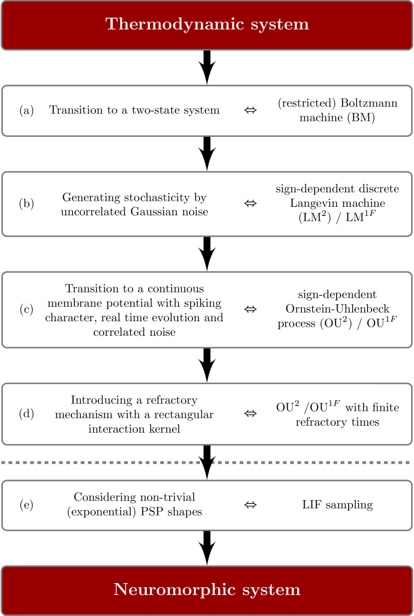
Figure 3: Illustration of a step-by-step approach to map thermodynamic systems on a neuromorphic hardware system. The dashed line indicates the progress of the paper. The paper proposes dynamics which have the potential to exactly preserve the properties of the Boltzmann machine up to this line.

In [22], an analytic expression for the neural activation function of leaky integrate-and-fire (LIF) neurons has been derived for the hardware of the BrainScaleS project in Heidelberg. It was demonstrated how the neuromorphic hardware system can be used to perform stochastic inference with spiking neurons in the high-conductance state. The microscopic dynamics of the membrane potential of a neuron can be approximated in this state with Poisson-driven LIF neurons by an Ornstein-Uhlenbeck process. The spiking character of the system is obtained by a threshold function which maps the system onto an effective two-state system.

Particular properties of LIF sampling are the following:

• A description of the microscopic state of a neuron by a continuous membrane potential,

• An autocorrelated noise contribution to the membrane potential,

• A spiking character with an asymmetric refractory mechanism and

• Nontrivial and nonconstant interaction kernels between neurons.

In the present section we study simplified dynamics of LIF sampling. This allows us to analyze the impact of particular hardware related properties and sources of resulting errors on different levels of abstraction. After a short introduction to the principles of LIF sampling, a mapping of the $\textnormal{LM}^{2}$ is presented with respect to several particularities of the hardware system. Possible sources of errors of the mapping are discussed. We also relate our approach to the standard approach which relies on a fit of the activation function of the hardware system to the activation function of the Boltzmann machine.

The section ends with an analysis of the impact of a refractory mechanism on the dynamics as a further step towards LIF sampling.

V.1 LIF sampling

The spikey neuromorphic system of the BrainScaleS project emulates spiking neural networks with physical models of neurons and synapses implemented in mixed-signal microelectronics [36, 22]. With the help of Poisson-driven leaky integrate-and-fire (LIF) neurons, it is possible to obtain stochastic inference with deterministic spiking neurons. The dynamics of the free membrane potential $u_{\textnormal{eff}}(t)$ of a neuron can be approximated in the high-conductance state by an Ornstein-Uhlenbeck process,

$$\frac{du_{\textnormal{eff}}(t)}{dt}=\theta\left[\mu-u_{\textnormal{eff}}(t)\right]+\sigma\tilde{\eta}(t)\,.$$ (21)

In (21), $\theta$ determines the strength of the attractive force towards the mean value $\mu=\mu^{\textnormal{leak}}+\mu^{\textnormal{average noise}}$. The mean value consists of some leak potential and an additional averaged noise contribution. The parameter $\sigma$ depends on the contribution of the Poisson background.

Inspired by a biological neuron [37], the neuron emits a spike when the membrane potential exceeds a certain threshold $\vartheta$. It is active and is reset to $\varrho$ for a refractory time $\tau_{\textnormal{ref}}$ afterwards, where the neuron is considered as inactive. This is also sketched in Figure 4. One has to distinguish between the effective membrane potential $u_{\textnormal{eff}}(t)$ (red curve), which is unaffected by the spiking dynamics, and the real membrane potential $u(t)$ (blue curve). As in [22], it is assumed that the convergence of $u(t)$ from $\varrho$ to $u_{\textnormal{eff}}(t)$ takes place in a negligible time after the finite refractory time has elapsed.

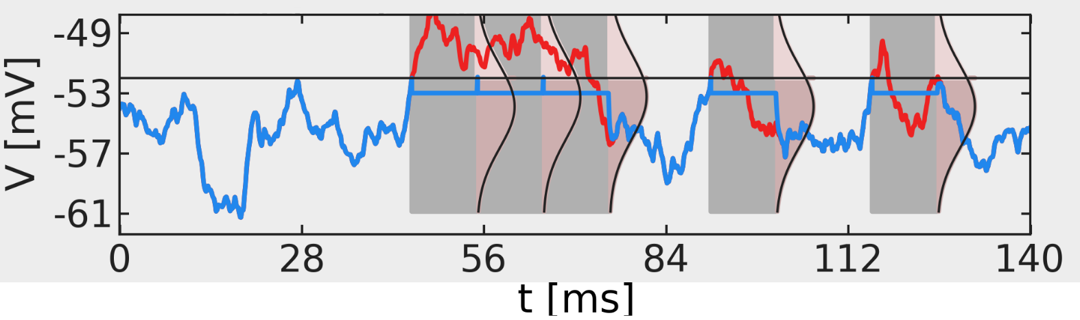
Figure 4: Example evolution of the free membrane potential (red) and the actual membrane potential (blue). After the membrane potential crosses the threshold $\vartheta$, a spike is emitted and the potential is set to a reset potential $\varrho$. If the effective membrane potential is still above $\vartheta$ after the refractory period $\tau_{\textnormal{ref}}$, the neuron spikes again. At the end of a "burst" of $n$ spikes the free and the actual membrane potential converge in negligible time (scheme taken from [37]).

V.1.1 Activation function

One can calculate distributions for the so-called burst lengths and the mean first passage times of the membrane potential with the help of transition probabilities $p(u_{i+1}|u_{i})$. These are given by a corresponding Fokker-Planck equation of the Ornstein-Uhlenbeck process in the high conductance state. The burst length $n$ is the number of consecutive spikes. The mean first passage time corresponds to the mean duration which it takes for the membrane potential to pass the threshold $\vartheta$ from a lower starting point. This is the time between an end of a burst and the next spike. From an iterative calculation one can derive an activation function, i.e., a probability distribution for the neuron to be active ($z=1$), in terms of these probabilities [22],

$$P(z=1)=\frac{\sum_{n}P_{n}n\tau_{\textnormal{ref}}}{\sum_{n}P_{n}\left(n\tau_{\textnormal{ref}}+\sum_{k=1}^{n-1}\overline{\tau_{k}^{b}}+T_{n}\right)}\,,$$ (22)

where $\overline{\tau_{k}^{b}}$ corresponds to the mean drift time from the resting potential $\varrho$ to $\vartheta$. The distribution over burst lengths is represented by $P_{n}$, and the distribution over the mean times between burst regimes is given by $T_{n}$.

V.1.2 A simplified model

If the refractory time $\tau_{\textnormal{ref}}$ is neglected, the neuron can be interpreted as active if the effective membrane potential is above a certain threshold, and as inactive otherwise. The resulting dynamics corresponds to the level of abstraction (c) in Figure 3. The neuron state is given by $z(t):=\Theta\left[u_{\textnormal{eff}}(t)-\vartheta\right]$. The process is referred to as an Ornstein-Uhlenbeck process with spiking character. Interacting contributions are implemented on the basis of the projected neuron states instead of their actual effective continuous membrane potential. The activation function is a cumulative Gaussian distribution,

$$P_{\textnormal{eq}}(z=1)=\int_{\vartheta}^{\infty}P_{\textnormal{eq}}(u_{\textnormal{eff}})\textnormal{d}u_{\textnormal{eff}}=\Phi\left(\frac{\sqrt{2\theta}}{\sigma}(\mu-\vartheta)\right)\,,$$ (23)

with the equilibrium distribution $P_{\textnormal{eq}}$ of the Ornstein-Uhlenbeck process (21),

$$P_{\textnormal{eq}}(u_{\textnormal{eff}})=\sqrt{\frac{\theta}{\pi\sigma^{2}}}\exp\left(-\frac{\theta(u_{\textnormal{eff}}-\mu)^{2}}{\sigma^{2}}\right)\,.$$ (24)

For convenience, the threshold potential $\vartheta$ is set to zero in further considerations.

The more accurate expression of the activation function, given by equation (22), takes the finite refractory time into account. The actual activation function is somewhere between a logistic distribution and the cumulative Gaussian distribution.

In the following, we neglect the finiteness of the refractory time. Therefore, we consider mostly simplified theoretical models of the hardware system of the level of abstraction (c). The models can be used to analyze Gaussian noise as stochastic input and the impact of autocorrelated noise in a system with a microscopic real time evolution of the membrane potential. Given by the spiking character, the considered models correspond effectively to interacting two-state systems. A discussion with respect to a refractory mechanism, as a process of the level of abstraction (d), is given in Section V.4.

V.2 Boltzmann machine

In this section we discuss a mapping of the Boltzmann machine (BM) onto an Ornstein-Uhlenbeck process with spiking character as a simplified model of a neuromorphic hardware system. A successful mapping demands a logistic distribution as activation function and a correct handling of interactions between neurons.

A possible approach is a fit of the activation function with a scaling parameter $r$ and a shift parameter $\mu^{0}$ to the desired logistic distribution according to $P_{\textnormal{eq}}(z=1)=\Phi\left(\frac{\sqrt{2\theta}}{\sigma}\frac{\mu-\mu^{0}}{r}\right)\approx\sigma\left(\mu\right)$, with $\sigma(x)=\left[1+\exp(-x)\right]^{-1}$ [22, 12, 20]. Interactions can be taken into account by absorbing their contributions into the mean value $\mu$ of the Ornstein-Uhlbenbeck process according to: $\mu\to\mu+\mu^{\textnormal{interaction}}$. It is assumed that the time to equilibrium is negligible after a change of an interacting neuron.

A mapping of the Boltzmann machine to a process of the level of abstraction (c) can be performed straightforwardly by identifying the total input (see Appendix E) of a neuron $i$ with the mean value $\mu_{i}$ of the Ornstein-Uhlenbeck process according to: $\mu_{i}\leftrightarrow-m_{i}$. This can be achieved by setting the average noise contribution to zero, adjusting the leak potential to $b_{i}$, and by taking the interacting contributions into account:

$$\mu_{i}^{\textnormal{average noise}} =0\,,$$

$$\mu_{i}^{\textnormal{leak}} =b_{i}\,,$$

$$\mu_{i}^{\textnormal{interaction}} =\sum_{\textnormal{syn}j}W_{ij}z_{j}(t)\,.$$ (25)

Then, from the dynamics of equation (21) with a correct scaling of the interaction strength (see Appendix F) the following Ornstein-Uhlenbeck process with spiking character is obtained:

$$\frac{du_{i,\textnormal{eff}}(t)}{dt} =$$

$$=\frac{\theta}{r^{2}} \left[\sum_{\textnormal{syn}j}W_{ij}z_{j}(t)+b_{i}-\mu_{i}^{0}-u_{i,\textnormal{eff}}(t)\right]+\sigma\tilde{\eta}(t)\,,$$ (26)

with $z_{j}(t)=\Theta\left[u_{j,\textnormal{eff}}(t)-\vartheta\right]$ and where $W_{ij}=\frac{A_{ij}}{\alpha}$ and $A_{ij}\to\frac{A_{ij}}{\alpha}$. With $\sigma=\sqrt{2}$, $\theta=1$ we obtain the following activation function:

$$P_{\textnormal{OU}^{1\textnormal{F}}}(z_{i}=1)=\Phi\left(\frac{\sum_{\textnormal{syn}j}W_{ij}z_{j}+b_{i}-\mu_{i}^{0}}{r}\right)\,.$$ (27)

The process is abbreviated in the following by $\textnormal{OU}^{1\textnormal{F}}$. The "1" in the exponent is chosen in compliance with the $\textnormal{LM}^{2}$ process and indicates that the process takes place in one regime, i.e., the process does not fluctuate between two fundamental dynamics. The fitting of the activation function to the logistic distribution is indicated by the additional "F". The process without any fitting parameters ($r=1$, $\mu_{i}^{0}=0$) is denoted as $\textnormal{OU}^{1}$.

We can also formulate an update rule with the same resulting activation function for a discrete two-state system, i.e., a system without a membrane potential. The resulting system is build upon an immediate representation of the neuron state, as it is the case for the BM and the $\textnormal{LM}^{2}$. The resulting process corresponds to a transition from the level of abstraction (c) to the level (b) and is driven by uncorrelated Gaussian noise.

The related update rule of level of abstraction (b) is derived in a similar manner as for the Langevin equation for discrete systems. It is given by,

$$z_{i}^{\prime}=\Theta\left[\sum_{\textnormal{syn}j}W_{ij}z_{j}+b_{i}+\tilde{\eta}\right]\,,$$ (28)

where the updates take place in computer time. The corresponding transition probability reads,

$$W_{\textnormal{LM}^{1\textnormal{F}}}(z_{i}\to 1)=\Phi\left(\frac{\sum_{\textnormal{syn}j}W_{ij}z_{j}+b_{i}-\mu_{i}^{0}}{r}\right)\,.$$ (29)

The dynamics has an additive Gaussian noise term and the Heaviside function as a projection onto the domain of definition of $z_{i}$. Therefore, it is very similar to the sign-dependent discrete Langevin machine (18). The update rule is studied in [19] in more detail and introduced in [10] as an approximation of the so-called Synaptic Sampling Machine. In compliance with the $\textnormal{LM}^{2}$ and the $\textnormal{OU}^{1}$, we use the abbreviation $\textnormal{LM}^{1}$ for the process. When the activation function is fitted to the logistic distribution, $\textnormal{LM}^{1\textnormal{F}}$ is the corresponding acronym. In the latter case, sources of errors are resulting deviations due to an imperfect fit and finite times to equilibrium if an interacting neuron changes its macroscopic state [19].

The dynamics can be interpreted as another realisation of the discrete Langevin machine, as will be discussed in Section VI. Properties and similarities of the two presented processes, i.e., the $\textnormal{LM}^{1}$ (28) and the $\textnormal{OU}^{1}$ (21) and (V.2), are numerically investigated in Section VII.

V.3 Sign-dependent Ornstein-Uhlenbeck process

The sign-dependent discrete Langevin machine and LIF neurons exhibit similar underlying dynamics. This motivates a mapping of the $\textnormal{LM}^{2}$ onto an Ornstein-Uhlenbeck process with spiking character in the same manner as in the previous section, i.e., from the level of abstraction (b) to (c). The resulting process represents a continuous counterpart to the sign-dependent discrete Langevin machine and is referred to as sign-dependent Ornstein-Uhlbenbeck process ($\textnormal{OU}^{2}$). The activation function of the $\textnormal{OU}^{2}$ process converges in the limit $\epsilon\to 0$ also to a logistic function. As illustrated in Figure 1, the two processes differ in their microscopic representation and their timescales. The $\textnormal{LM}^{2}$ corresponds to a process with two discrete states and the computer time as timescale. The $\textnormal{OU}^{2}$ process describes the temporal evolution of a membrane potential in real time, whereas the interactions between neurons are based on a projection of the potential onto two states.

The total input $\sum_{j}W_{ij}z_{j}+b_{i}$ of the dynamics of the previous section is exchanged for a mapping onto an Ornstein-Uhlenbeck process by the redefined membrane potential of the sign-dependent discrete Langevin machine: $W^{\prime}_{ii}z_{i}+\sum_{j}W^{\prime}_{ij}z_{j}+b^{\prime}_{i}$. This leads to the following dynamics of the sign-dependent Ornstein-Uhlenbeck process:

$$\frac{du_{i,\textnormal{eff}}(t)}{dt} =$$

$$=\theta \left[W^{\prime}_{ii}z_{i}(t)+\sum_{\textnormal{syn}j}W^{\prime}_{ij}z_{j}(t)+b^{\prime}_{i}-u_{i,\textnormal{eff}}(t)\right]$$

$$+\sigma\tilde{\eta}(t)\,,$$ (30)

with $z_{i}(t)=\Theta\left[u_{i,\textnormal{eff}}(t)-\vartheta\right]$. The additional scaling factor of $\lambda_{\epsilon}$ is omitted, i.e., it holds: $W_{ii}^{\prime}=\frac{2}{\sqrt{\epsilon}}$, $W_{ij}^{\prime}=\frac{\sqrt{\epsilon}}{2}W_{ij}$, and $b_{i}^{\prime}=\left(\frac{\sqrt{\epsilon}}{2}b_{i}-\frac{1}{\sqrt{\epsilon}}\right)$. The term sign-dependent reflects again the property of the neuron to stay very long in an active regime ("$+$"), or in an inactive regime ("$-$"). If the membrane potential randomly crosses the threshold $\vartheta$, it perceives a strong drift towards the other regime, due to the changing mean value of the process, i.e., due to the transition $z_{i}=0\to z_{i}=1$. An immediate return to its initial regime gets rather unlikely because of the dependence of the mean value on $\frac{1}{\sqrt{\epsilon}}$. This property is reflected by the characteristic dynamics of the process which is shown in the lower left part of Figure 5.

[mode=buildnew]distributionnorefractory_prx

[mode=buildnew]distributionrefractory

Figure 5: Upper plots: Comparison of equilibrium distributions $P_{\textnormal{eq}}(u_{i,\textnormal{eff}})$ for the continuous processes for the free case with bias $b=0.8$ without a refractory mechanism (a) and with a refractory mechanism with refractory time $\tau_{\textnormal{ref}}=8$ (b). Lower plots: Corresponding example trajectories of the $\textnormal{OU}^{2}$ processes with and without a refractory mechanism for $\epsilon=0.2$. The timescale of the lower plot is rescaled according to the transition probabilities to coincide.

The equilibrium distribution over $u_{i,\textnormal{eff}}(t)$ of the process is derived in Appendix D. It is given by

$$P_{\textnormal{eq}}(u_{i,\textnormal{eff}})\propto\exp\left[K(u_{i,\textnormal{eff}})\right]\,,$$ (31)

with

$$K (u_{i,\textnormal{eff}})=$$

$$=\frac{|u_{i,\textnormal{eff}}|}{\sqrt{\epsilon}}+\frac{\sqrt{\epsilon}}{2}\left(\sum_{\textnormal{syn}j}W_{ij}z_{j}+b_{i}\right)u_{i,\textnormal{eff}}-\frac{u_{i,\textnormal{eff}}^{2}}{2}\,.$$ (32)

The exponent $K(u_{i,\textnormal{eff}})$ contains the absolute value of the effective potential. This property causes a change of the sign of the resulting Gaussian distribution in dependence of the sign of $u_{i,\textnormal{eff}}$. Therefore, the equilibrium distribution can be considered as the concatenation of two Gaussian distributions $P_{\textnormal{eq}}^{+}(u_{i,\textnormal{eff}})$ and $P_{\textnormal{eq}}^{-}(u_{i,\textnormal{eff}})$ with different mean values. In the active regime, the resulting mean value is $\mu_{i}^{+}(t)=-\frac{1}{\sqrt{\epsilon}}-\frac{\sqrt{\epsilon}}{2}\left(\sum_{\textnormal{syn}j}W_{ij}z_{j}(t)+b_{i}\right)$ and in the inactive regime, it holds $\mu_{i}^{-}(t)=-\frac{1}{\sqrt{\epsilon}}+\frac{\sqrt{\epsilon}}{2}\left(\sum_{\textnormal{syn}j}W_{ij}z_{j}(t)+b_{i}\right)$. The two distribution are reweighted according to the resulting overall stationary probability distribution. The left part of Figure 5 compares numerically found stationary distributions with the analytical result of equation (31).

The stationary distribution of the process as a function of $z_{i}$ can be obtained by an integration of $P_{\textnormal{eq}}(u_{i,\textnormal{eff}})$ over $u_{i,\textnormal{eff}}$ with respect ot the threshold $\vartheta$. As derived in Appendix D, this results in the following activation function of the sign-dependent Ornstein-Uhlenbeck process,

$$P_{\textnormal{OU}^{2}}(z_{i}=1)=\frac{1}{1+\exp\left[\alpha_{\epsilon}(m_{i})\times m_{i}\right]}\,,$$ (33)

with $\alpha_{\epsilon}(m_{i})$ being a correction factor. Here, $m_{i}:=-\sum_{\textnormal{syn}j}W_{ij}z_{j}(t)-b_{i}$ corresponds to the total input of the neuron. Since $\lim\limits_{\epsilon\to 0}\alpha_{\epsilon}(m_{i})=1$, the activation function converges in the limit of $\epsilon\to 0$ to the logistic distribution,

$$\lim\limits_{\epsilon\to 0}P_{\textnormal{OU}^{2}}(z_{i}=1)=\frac{1}{1+\exp\left[-\sum_{\textnormal{syn}j}W_{ij}z_{j}-b_{i}\right]}\,,$$ (34)

the activation function of the Boltzmann machine. The correction factor $\alpha_{\epsilon}(m_{i})$ is different to the scaling factor $\lambda_{\epsilon}$ of the $\textnormal{LM}^{2}$ since the convergence to the logistic distribution is caused by different characteristics for the two processes. Figure 6 compares numerically found scaling and correction factors of the $\textnormal{LM}^{2}$ and $\textnormal{OU}^{2}$ process with the theoretical factors $\lambda_{\epsilon}$ and $\alpha_{\epsilon}(m_{i})$ for different biases $b$ in the free case, i.e., for the activation function.

The overlap of the tails of the two shifted Gaussian distributions is responsible for the correction factor. The two distributions do not overlap at all in the limit of $\epsilon\to 0$. Hence, the activation function corresponds to the logistic distribution only in this case. For larger values of $\epsilon$, the distributions are closer together and crossings between the active and the inactive state take place more often. This property results in deviations to the logistic distribution.

[mode=buildnew]ScalingLM2

[mode=buildnew]ScalingOU2PRX

Figure 6: Comparison of scaling and correction factors for the sign-dependent processes for a better convergence to the logistic distribution: (a) The numerical and the analytic scaling factor $\lambda_{\epsilon}=\lambda\left(\sqrt{\epsilon}\right)$ for the sign-dependent Langevin machine. (b) The numerical and analytic correction factors $\alpha_{\epsilon}$ for the sign-dependent Ornstein-Uhlenbeck process.

An advantage of the sign-dependent Ornstein-Uhlenbeck process is the possibility to extrapolate results for different values of $\epsilon$ to the limit of $\epsilon\to 0$, i.e., to exact results of the Boltzmann machine. A disadvantage of the process is that smaller values of $\epsilon$ lead to larger correlation times and therefore to a higher simulation cost. This results from the limitation that it is not possible to accelerate the dynamics by an adaptation of the noise source, as it is the case for the $\textnormal{LM}^{2}$. From another perspective, this property might even help to straighten out problems related to the hardware, like nontrivial postsynaptic shapes, for example.

A comparison of the dynamics in (V.3) with the mapping of the Boltzmann machine in equation (V.2) shows that the self-interaction and the dynamics of the discrete Langevin machine are key ingredients for a successful mapping onto the spiking system. The properties of the $\textnormal{OU}^{2}$ process are dominated essentially by the self-interacting term. Therefore, the process is not just an Ornstein-Uhlenbeck process, but represents a kind of dynamics with a different resulting equilibrium distribution and, up to now, noninvestigated properties. Similar dynamics which contain projected values of interacting potentials might serve as a starting point for an entire class of dynamics.

V.4 Refractory mechanism

A possible further step towards LIF sampling is to take into account a refractory mechanism. This step is given in Figure 3 by the level of abstraction (d). The refractory mechanism can be also considered for a discrete system, for example, for the Boltzmann machine. This approach represents a different ordering of the different abstractions of Figure 3.

In a simplified model, it can be assumed that a neuron stays active for the refractory time $\tau_{\textnormal{ref}}$, after it got activated. An imbalance between the active and the inactive state is caused by this property. This asymmetry can be compensated by reducing the transition probability to become active by a factor of $1/\tau_{\textnormal{ref}}$, as discussed in [21]. The factor can be absorbed into the membrane potential by a shift of the activation function by $\log\left(\tau_{\textnormal{ref}}\right)$, i.e., by $b_{i}\to b_{i}-\log\left(\tau_{\textnormal{ref}}\right)$. Note that the sign-dependent processes lead to a reformulation of the neuron computability condition of [21] due to the inherent dependency of the dynamics on the neuron state itself.

[mode=buildnew]activationfunction1ref

Figure 7: Illustration of the nonsymmetric deformation of the $\textnormal{LM}^{1}$ and the $\textnormal{OU}^{1}$ process for larger refractory times. The activation functions are shifted to comply: $P(z_{i}=1)\big{|}_{b=0}=0.5$. The small plot contains the absolute deviation to the cumulative Gaussian distribution.

For the cumulative Gaussian distribution, an absorption of the factor of $1/\tau_{\textnormal{ref}}$ is not possible anymore. The resulting activation function with a finite refractory time is deformed. The deformation gets larger for larger refractory times, as can be seen in Figure 7. We conclude that the errors of the activation function to the logistic distribution without a refractory mechanism propagate and increase for dynamics with finite refractory times $\tau_{\textnormal{ref}}$. The resulting deformation of the activation function can be identified as a further source of error.

Within the last level of abstraction of Figure 3, interactions between neurons or with the neuron itself are in general not constant. The so-called postsynaptic potential (PSP) corresponds to the received input potential of an interacting neuron [22]. In Appendix F, the relation between a correct implementation of the weights based on the interaction kernel is discussed in more detail. In this work, only rectangular PSP shapes are considered. An investigation of exponential PSP shapes is postponed to future work.

It is important to distinguish between the refractory mechanism as a property of each neuron itself and the postsynaptic potential. The latter needs only to be taken into account if interactions between neurons are considered. In particular, this means that the PSP shape affects only the activation function of the sign-dependent processes due to their self-interacting contribution.

	Gibbs sampling (BM)	$\textnormal{{LM}}^{\textnormal{{1F}}}$	$\textnormal{{LM}}^{\textnormal{{2}}}$	$\textnormal{{OU}}^{\textnormal{{1F}}}$	$\textnormal{{OU}}^{\textnormal{{2}}}$	$\textnormal{{LM}}^{\textnormal{{1}}}$	$\textnormal{{OU}}^{\textnormal{{1}}}$
Activation function	Logistic distribution	$\approx$ Logistic distribution	$\approx$ Logistic distribution	$\approx$ Logistic distribution	$\approx$ Logistic distribution	Cumulative Gaussian distribution	Cumulative Gaussian distribution
Microscopic representation	Discrete	Discrete	Discrete	Continuous	Continuous	Discrete	Continuous
Timescale	Computer time	Computer time	Computer time	Real time	Real time	Computer time	Real time
Deviations (free case)	Exact	Small	Small	Small	Small	Exact	Exact
Extrapolation to exact solution?	-	No	Yes	No	Yes	-	-
Deviations (interacting case)	Exact	Medium	Small	Large	Small	Exact	Exact
Extrapolation to exact solution?	-	No	Yes	No	Yes	-	-
Control of a refractory mechanism	Exact [21]	Constant shift $\tau(\tau^{\prime})$	Constant shift $\tau(\tau^{\prime})$	Constant shift $\tau(\tau^{\prime})$	Constant shift $\tau(\tau^{\prime})$	Nontrivial shift $\tau(\tau^{\prime},W_{ij},b_{i})$	Nontrivial shift $\tau(\tau^{\prime},W_{ij},b_{i})$

Table 1: Comparison of the different analysed dynamics. An extrapolation to the exact solution and, therefore, a control of sources of errors is possible for the $\textnormal{LM}^{2}$ and the $\textnormal{OU}^{2}$ for both with and without a refractory mechanism.

VI Discrete Langevin machine

The Ornstein-Uhlenbeck process with a spiking dynamics and correlated noise offers the possibility to simulate a discrete two-state system by an underlying continuous dynamics. The discrete Langevin machine can be interpreted as a discrete counterpart to those spiking systems with uncorrelated noise, as indicated in Figure 1. It has been shown, that it is possible to map different realisations of simplified theoretical models of the neuromorphic hardware system onto a two-state system (see Figure 3 as well as the dynamics (V.2) $\leftrightarrow$  (28) and (V.3) $\leftrightarrow$ (18)). Denoting the hardware as $\textnormal{HW}(p)$, with parameters $p=\{W_{ij},b_{i},z_{i},\epsilon\}$, and the discrete Langevin machine as $\textnormal{LM}(h)$, with $h:=h(p)$, we can state the important relation,

$$\{\textnormal{LM}(h)\}=\{\textnormal{HW}(p)\}\,,$$ (35)

i.e., there exists a discrete two-state system for each set of parameters $p$ of the hardware which emulates the dynamics of the spiking system in discrete space.

In terms of update dynamics this corresponds to the mapping of

$$\frac{du_{i,\textnormal{eff}}(t)}{dt}=\theta\left[\mu_{i}(p)-u_{i,\textnormal{eff}}(t)\right]+\sigma\tilde{\eta}(t)\,,$$ (36)

onto a discrete dynamics

$$z_{i}^{\prime}=\Theta\left[\mu_{i}(h(p))+\tilde{\eta}\right]\,,$$ (37)

for all realisations of $p$ and with $z_{i}=\Theta\left[u_{i,\textnormal{eff}}(t)\right]$.

Relation (35) and the formal introduction of the discrete Langevin machine can be seen as a theoretical framework to describe different possible implementations as well as several levels of abstraction of LIF sampling in terms of processes in real time with a continuous membrane potential and spiking character and processes in computer time with discrete states. For an exact mapping $h(p)$, the magnitudes of the sources of error have to be matched. Table 1 gives an overview of the presented theoretical models and their properties regarding different levels of abstraction of a neuromorphic system.

VII Applications

[mode=buildnew]magnclock

[mode=buildnew]spehclock

Figure 8: Comparison of the magnetization (a) and the specific heat (b) obtained by a standard Monte Carlo algorithm and by the $\textnormal{LM}^{2}$ for the 4-state clock model on a $16\times 16$ lattice. The results of the $\textnormal{LM}^{2}$ converge for $\epsilon\to 0$ to the results of the standard Monte Carlo algorithm. Relative deviations of the inverse critical temperatures in dependence of $\epsilon$ are illustrated in Figure 9.

Numerical results are discussed for the Langevin equation for discrete systems of Section III, for the introduced sign-dependent Ornstein-Uhlenbeck process as well as for existing approaches. We start with an analysis of the clock model in Section VII.1. Dynamics and equilibrium distributions of the free membrane potential are compared in Sections VII.2 and VII.3 for the discrete Langevin machine and for abstractions of the neuromorphic hardware system, according to Figure 3 and Table 1. The focus is on a correct implementation of the logistic distribution of the Boltzmann machine and on a detailed analysis of the impact of different sources of errors. The systems are considered with and without an asymmetric refractory mechanism with a rectangular postsynaptic shape. The section ends with a computation of the Ising model by a projection of the model on the Boltzmann machine and with a numerical investigation of a Boltzmann machine with three neurons in Section VII.4. Both models serve as a benchmark for Boltzmann distributed systems with interacting neurons.

[mode=buildnew]errorscrit

Figure 9: Relative deviations of the obtained inverse critical temperatures for finite values of $\epsilon$ to the inverse critical temperature of a standard Monte Carlo algorithm.

VII.1 $q$-state clock model

The $q$-state clock model [38, 39] describes spins $\theta_{i}=\frac{2\pi n}{q}$ with $q$ different states which are parametrised by $n\in\{1,2,\dots,q\}$. It is used to verify numerically the Langevin equation for discrete systems, as a first example. The model has the following Hamiltonian:

$$H_{c}=-J_{c}\sum_{\langle i,j\rangle}\cos\left(\theta_{i}-\theta_{j}\right)\,.$$ (38)

The sum runs over all nearest neighbor spin pairs $\langle i,j\rangle$. In a complex plane one can interpret the spin states as equally distributed states on an unit circle. The common Potts model [40] is derived from this initial model. For $q=2$ the model corresponds to the Ising model and in the limit of $q\to\infty$, it describes the continuous $XY$ model. For $q=4$ the system emulates two independent Ising models.

The clock model exhibits for $q\leq 4$ a second order phase transition. It exists an exact solution for the inverse critical temperature for $q=4$, which is as follows [41]:

$$J_{c}\beta_{c}^{q=4}=2J_{c}\beta_{c}^{q=2}\,,$$ (39)

where the Boltzmann constant $k_{b}$ has been set to $1$. An appropriate order parameter for the system is the average magnetization per spin, which can be defined as

$$m=\frac{1}{N}\bigg{|}\sum_{k}^{N}e^{\frac{i2\pi n_{k}}{q}}\bigg{|}\,,$$ (40)

where the sum runs over all spins $n_{k}$ of a lattice with $N$ sites. The specific heat capacity $c$ per spin is considered as a further observable and is defined as

$$c=\frac{\beta^{2}}{N}\left(\langle E^{2}\rangle-\langle E\rangle^{2}\right)\,,$$ (41)

where $\langle\cdot\rangle$ denotes the expectation value [42].

Numerical results for the magnetization and the specific heat are illustrated in Figure 8 in dependency of the inverse temperature $\beta$ and of different values of $\epsilon$. Results of the Metropolis algorithm as a standard Monte Carlo algorithm (MC) serve as benchmark. The inverse critical temperature can be read off from the maximum of the specific heat. In Figure 9, the relative deviations of the inverse critical temperature to the inverse critical temperature of the Metropolis algorithm are plotted against $\epsilon$.

The resulting deviations for finite values of $\epsilon$ can be explained by a detailed error analysis of the transition probabilities of the Langevin equation for discrete systems. For this purpose, one has to check the compliance of the detailed balance equation,

$$\frac{W_{\textnormal{LM}^{2}}(\theta\to\theta^{\prime})}{W_{\textnormal{LM}^{2}}(\theta^{\prime}\to\theta)}+\mathcal{O}\left(\epsilon\Delta H_{c}(\theta^{\prime},\theta)^{3}\right)=\frac{P_{\textnormal{MC}}(\theta^{\prime})}{P_{\textnormal{MC}}(\theta)}\,.$$ (42)

In the left part of Figure 16, it can be seen that the absolute error of the cumulative Gaussian distribution is asymmetric around $x=0$. This imbalance leads to a shift of the effective fraction of transition probabilities and therefore to a change of the equilibrium distribution of the spin states. The strength of this shift grows for larger values of $x$, which corresponds to larger values of $\beta\Delta H_{c}$, and larger values of $\epsilon$. The effect can be nicely observed in the change of the specific heat in the right part of Figure 8 with growing $\beta$. In general, it holds: the larger $|\beta\Delta H_{c}|$, the worse is the compliance of the detailed balance equation and the larger is the resulting shift of the equilibrium distribution.

[mode=buildnew]AFlogistic

[mode=buildnew]AFlogisticRef

[mode=buildnew]divepsilonuaf

[mode=buildnew]divtauaf

Figure 10: Comparison of different properties of the activation function for the different processes with and without a refractory mechanism: (a) Activation function and absolute deviation to the logistic distribution without a refractory mechanism. (b) The same as in (a), but with a refractory mechanism with refractory time $\tau=8$. (c) Absolute deviation of the exact results of the activation for $b=1$ for the sign-dependent processes in dependence of $\epsilon$. The deviation converges in the limit $\epsilon\to 0$ for all processes to zero, with and without a refractory mechanism. (d) Absolute deviation of the results for the $\textnormal{OU}^{2}$ process without a refractory mechanism to results with a refractory mechanism and different values of $\tau_{\textnormal{ref}}$. The deviations are compared for $b=\{-1,0,1\}$.

VII.2 Neuromorphic hardware versus Langevin machine

We analyze numerically the mapping between dynamics of the discrete Langevin machine and the continuous dynamics according to relation (35) by an explicit consideration of transition probabilities. It is discussed the impact of deviations in the transition probabilities as well as a mapping of the temporal evolution of the different processes onto each other with respect to resulting activation functions for the free membrane potential.

Differences of the two dynamics which are given by construction are illustrated in Figure 1. The processes correspond to the levels of abstraction (b) and (c) of a neurmorphic hardware system in Figure 3. The essential differences are the source of noise, which is for the Langevin machine uncorrelated and for the Ornstein-Uhlenbeck process correlated, as well as the representation of a microscopic state. The dynamics is described in the former case by two discrete states in computer time and in the latter one by the evolution of a continuous membrane potential with spiking character in real time. We evaluate the impact of the different sources of errors on the deviation to the expected logistic distribution for the sign-dependent and for the fitted processes: $\textnormal{LM}^{2}$, $\textnormal{OU}^{2}$, $\textnormal{LM}^{\textnormal{1F}}$, and $\textnormal{OU}^{\textnormal{1F}}$.

VII.2.1 Activation function

Figure 7 and the upper left part of Figure 10 illustrate the activation functions of the free membrane potential in dependency of the bias $b$ in the network for the different presented dynamics. The results of the $\textnormal{LM}^{1}$ and the $\textnormal{OU}^{1}$ process coincide exactly and their deviation to the cumulative Gaussian distribution emerges from numerical errors. In concordance to these observations, the fitted $\textnormal{LM}^{1\textnormal{F}}$ and $\textnormal{OU}^{1\textnormal{F}}$ process have the same deviations to the logistic distribution. In the case of the $\textnormal{LM}^{2}$ and the $\textnormal{OU}^{2}$ process, the observed deviations mirror the theoretical errors for finite values of $\epsilon$. As depicted in the lower left part of Figure 10, both activation functions converge in the limit of $\epsilon\to 0$. The rate of convergence of the $\textnormal{OU}^{2}$ process is much smaller than the one of the $\textnormal{LM}^{2}$ for equal values of $\epsilon$. This can be reasoned by the different sources of errors for the two processes, as discussed in detail at the ends of Sections IV and V.3. In contrast to the $\textnormal{LM}^{1\textnormal{F}}$ and $\textnormal{OU}^{1\textnormal{F}}$, deviations to the logistic distribution are limited only due to larger correlation times for smaller values of $\epsilon$ for the $\textnormal{OU}^{2}$ process.

VII.2.2 Dynamics: time evolution

[mode=buildnew]trajectories

Figure 11: Trajectories of the neuron state and the membrane potential in computer time for the different processes with a uniform timescale.

It has been found numerically that the computer time and the real time coincide for the $\textnormal{LM}^{1}$ and the Ornstein-Uhlenbeck process. All simulations in real time are performed with finite time steps of $0.02$. All processes in computer time are computed with a random sequential update formalism and in real time by a parallel update scheme. The timescale in all figures is chosen in units of the computer time.

Figure 11 compares trajectories of the different discussed processes with respect to a uniform timescale. It can be observed in the evolution of the membrane potential for all processes that there occur fast changes if the membrane potential is close to the threshold value $\vartheta=0$. These perturbations seem to have no influence on the time evolution and the equilibrium distribution.

As discussed in Section III, a scaling factor $a$ can be found for a correct mapping of the temporal evolution of two processes A and B if both processes exhibit the same equilibrium distribution. The scaling factor is given under usage of equation (15) and by a computation of the transition probabilities by

$$a=\frac{W_{\textnormal{A}}(0\to 1)}{W_{\textnormal{B}}(0\to 1)}\,.$$ (43)

Analytic expressions for the transition probabilities of the considered sign-dependent processes are given in Table 2. The given transition probabilities have been validated numerically. For that purpose we have mapped the temporal ensemble evolution of the different dynamics onto the evolution of the Boltzmann machine with respect to the computed scaling factors. A scaling factor $a\neq 1$ reflects the increase/decrease of the correlation time for processes with different transition probabilities. In Figure 12, the dependency of the scaling factor $a$ on $\epsilon$ is plotted for the sign-dependent processes.

The considerations of the time evolution reinforce that the relation of equation (35) corresponds to an exact mapping of the dynamics of a discrete system with uncorrelated noise to a continuous system with correlated noise. This property is not self-evident. However, the dependency $h(p)$ is in some cases nontrivial, due to different occurring sources of errors of the considered models.

VII.3 Refractory mechanism

In this section we investigate the impact of an asymmetric refractory mechanism of a neuromorphic system with a rectangular PSP shape. This has been introduced in Section V.4 as the level of abstraction (d) with regard to Figure 3.

VII.3.1 Control of the refractory mechanism

We concentrate on a correct representation of the logistic function with a refractory mechanism. The imbalance between the inactive and the active state can in general not be compensated entirely by a trivial shift of the bias by $\log\left(\tau_{\textnormal{ref}}\right)$ for the cumulative Gaussian distribution. The activation functions of the sign-dependent processes and the fitted dynamics are close to a logistic distribution. Therefore, a shift can be used to approximate the logistic distribution with a refractory mechanism. However, for large refractory times this approximation gets worse, as indicated in Figure 7.

	$W_{\textnormal{BM}}(0\to 1)$	$W_{\textnormal{LM}^{2}}(0\to 1)$	$W_{\textnormal{OU}^{2}}(0\to 1)$
$\tau_{\textnormal{ref}}=1$	$\sigma(-m_{i})$	$\Phi\left(-\frac{1}{\sqrt{\epsilon}}-\frac{\sqrt{\epsilon}}{2\lambda_{\epsilon}}m_{i}\right)$	$\varphi\left(-\frac{1}{\sqrt{\epsilon}}-\frac{\sqrt{\epsilon}}{2}m_{i}\right)$
$\tau_{\textnormal{ref}}>1$	$\sigma(-\left(m_{i}+\log(\tau_{\textnormal{ref}})\right))$	$\Phi\left(-\frac{1}{\sqrt{\epsilon}}-\frac{\sqrt{\epsilon}}{2\lambda_{\epsilon}}(m_{i}+\log(\tau_{\textnormal{ref}}))\right)$	$\varphi\left(-\frac{1}{\sqrt{\epsilon}}-\frac{\sqrt{\epsilon}}{2}(m_{i}+\log(\tau_{\textnormal{ref}}))\right)$

Table 2: Transition probabilities from an inactive state to an active state for the different considered dynamics with ($\tau_{\textnormal{ref}}>1$) and without ($\tau_{\textnormal{ref}}=1$) a refractory time. $m_{i}$ corresponds to the total input for a neuron $i$, according to Appendix E.

In this work, the shift of the activation function is determined by the constraint that $p(z_{i}=1)\big{|}_{b=0}=0.5$. The actual shifts of the bias are slightly different for the $\textnormal{LM}^{\textnormal{1F}}$ and the $\textnormal{OU}^{\textnormal{1F}}$ as a consequence of resulting deformations of the cumulative Gaussian distribution for larger refractory times (see Figure 7). We also introduce a further time constant $\tau_{\textnormal{ref}}^{\prime}$. This allows us to distinguish clearly between the refractory time $\tau_{\textnormal{ref}}$ of a neuron and the resulting optimal shift $\log(\tau_{\textnormal{ref}}^{\prime})$ for a correct fixing of the activation function. Ideally, one should derive a dependency $\tau_{\textnormal{ref}}^{\prime}(\tau_{\textnormal{ref}})$ to preserve a consistent fixing of the activation function.

For the $\textnormal{LM}^{2}$ process it holds true that $\tau_{\textnormal{ref}}\simeq\tau_{\textnormal{ref}}^{\prime}$, since the deviation of the activation function to the logistic distribution is nearly symmetric around $b=0$. Nevertheless, a shift by $\log(\tau_{\textnormal{ref}}^{\prime})$ leads to a worse approximation of the transition probability, since the Taylor expansion of the cumulative Gaussian distribution of the $\textnormal{LM}^{2}$ dynamics is performed around $0$. This is a further error source.

[mode=buildnew]correlation_times_bias0

Figure 12: Scaling factors $a$ in dependence of $\epsilon$ for a mapping of the transition probabilities of the sign-dependent processes onto the transition probability of the Boltzmann machine and, hence, of the temporal evolution on the computer time. The scaling factors are computed for the free case with a bias $b=0$.

For the $\textnormal{OU}^{2}$ process, the necessary shift of the bias by $\log\left(\tau_{\textnormal{ref}}^{\prime}\right)$ is much larger than $\log\left(\tau_{\textnormal{ref}}\right)$. Dependencies of $\tau_{\textnormal{ref}}^{\prime}(\tau_{\textnormal{ref}})$ for fixed values of $\epsilon$ and $\tau_{\textnormal{ref}}^{\prime}(\epsilon)$ for $\tau_{\textnormal{ref}}=8$ are illustrated in Figure 13. The large differences in $\tau_{\textnormal{ref}}$ and in $\tau_{\textnormal{ref}}^{\prime}$ can be traced back to the different microscopic dynamics of the processes and to the different origin of a correct implementation of the activation function for the processes without a refractory mechanism.

In contrast to the $\textnormal{OU}^{1}$ process, the dynamics of the $\textnormal{OU}^{2}$ process fluctuates between the active and the inactivate regime which are distinguished and driven by the self-interacting contribution. Integrating a refractory mechanism, a change from the active to the inactive regime by the self-interacting term is suppressed as long as the neuron is captured in its refractory mode. This can be seen in the lower right plot of Figure 5. Consequently, the two Gaussian distributions, $P_{\textnormal{eq}}^{+}(u_{i,\textnormal{eff}})$ and $P_{\textnormal{eq}}^{-}(u_{i,\textnormal{eff}})$, have a dissimilar impact on the resulting distribution of $P(u_{i,\textnormal{eff}})$. The lower tail distribution of $P_{\textnormal{eq}}^{+}(u_{i})$, i.e., the part of the distribution for $u_{i,\textnormal{eff}}<\vartheta$, biases the distribution $P(u_{i,\textnormal{eff}})$ around the threshold $\vartheta=0$ within the refractory time. In contrast, the upper tail distribution of $P_{\textnormal{eq}}^{-}(u_{i,\textnormal{eff}})$ does not affect $P(u_{i,\textnormal{eff}})$, since the dynamics changes for $u_{i,\textnormal{eff}}>\vartheta$ from the inactive to the active regime. The local minimum of $P(u_{i,\textnormal{eff}})$ around $u_{i,\textnormal{eff}}=\vartheta$ as well as the entire distribution $P(z_{i})$ are shifted to smaller values, as a result of this asymmetry, as illustrated in the upper right part of Figure 5. Further, the absolute value of the minimum is larger than the one for the process without a refractory mechanism. The imbalance between $P_{\textnormal{eq}}^{+}(u_{i,\textnormal{eff}})$ and $P_{\textnormal{eq}}^{-}(u_{i,\textnormal{eff}})$ results in larger deviations of the activation function for the $\textnormal{OU}^{2}$ process with a refractory mechanism. This asymmetry corresponds to a further source of error.

The equilibrium distribution needs to undergo a larger shift by $\log(\tau_{\textnormal{ref}}^{\prime})$ than the $\textnormal{OU}^{1\textnormal{F}}$ process for a compensation of the impact of the refractory mechanism. This is a consequence of a partially suppression of the change of the dynamics to the inactive regime. For the $\textnormal{OU}^{1\textnormal{F}}$ process, the underlying dynamics is not affected by the refractory mode due to the absence of a self-interacting term. Therefore, the only purpose of the shift by $\log\tau_{\textnormal{ref}}^{\prime}$ is to fix the transition probabilities to correctly compensate the emerging asymmetry of the refractory mechanism. Respectively, the resulting transition probabilities are expressed in dependence of $\log(\tau_{\textnormal{ref}})$. Analytic expressions for the sign-dependent dynamics are given in Table 2.

[mode=buildnew]taurefvstaup

[mode=buildnew]epsilonvstaup

Figure 13: $\tau_{\textnormal{ref}}^{\prime}$ in dependence of the refractory time $\tau_{\textnormal{ref}}$ for $\epsilon=0.2$ and $\epsilon=0.5$ (a) and of $\epsilon$ for $\tau_{\textnormal{ref}}=8$ (b) for the $\textnormal{OU}^{2}$ process. Both dependencies obey a power law.

VII.3.2 Activation function and time evolution

The upper right part of Figure 10 compares the impact of a refractory mechanism on the different dynamics regarding their deviations to the logistic distribution. The deviations of the $\textnormal{LM}^{2}$ and the $\textnormal{OU}^{2}$ process have increased, as expected by the introduced asymmetry of the refractory mechanism. Nevertheless, the error vanishes for $\epsilon\to 0$, as illustrated in the lower left part of Figure 10. Further, the lower right part of Figure 10 shows that a further increase of the refractory time has a very low impact on the deviations which ensures an applicability for large refractory times, in practice. As discussed in Section V.4, the cumulative Gaussian distribution is nonsymmetrically deformed by the shift by $\log(\tau^{\prime})$. This leads to deviations in the activation function of the $\textnormal{LM}^{1}$ and the $\textnormal{OU}^{1}$ process that can be compensated to a certain extent by an adaptation of the variance, i.e., of the scaling parameter $r$.

We conclude that a refractory mechanism with rectangular PSP shape has no impact on a possible control of the sources of errors for the sign-dependent processes.

VII.4 Interacting systems

We consider the Ising model [43] and the Boltzmann machine [44] to investigate the presented abstractions of a neuromorphic hardware system with interactions between neurons. The Ising model can be easily mapped onto the Boltzmann machine. A numerical analysis can be understood as a proof of concept that the presented processes also work in a more complex network setup. As a second model, we study a Boltzmann machine with three neurons. We compare the results for all presented models with and without a refractory mechanism with a rectangular PSP shape.

The Ising model describes a two-state spin system. The spin states are $s_{i}\in\{-1,+1\}$, which are likewise also referred to as spin up and spin down $s_{i}\in\{\downarrow,\uparrow\}$. The Hamiltonian is defined as

$$H=-J\sum_{\langle i,j\rangle}s_{i}s_{j}-h\sum_{i}s_{i}\,.$$ (44)

The external magnetic field $h$ is set to zero in the following numerical analysis and $J=1$ is some coupling constant. For this particular case, we can consider the averaged absolute value of the magnetization per spin as an order parameter. This is then given by

$$m=\frac{1}{N}\bigg{|}\sum_{i}^{N}s_{i}\bigg{|}\,,$$ (45)

where the sum runs again over all spins of the lattice for a given configuration. From theoretical considerations, an exact expression for the inverse critical temperature of the model with a vanishing external field can be obtained [45],

$$J\beta_{c}=\frac{\ln\left(1+\sqrt{2}\right)}{2}\,.$$ (46)

For a computation with the presented algorithms, we need a mapping between the Boltzmann machine and the Ising model onto the correct domain of definition. The mapping of $s_{i}=-1\to z_{i}=0$ and $s_{i}=1\to z_{i}=1$ can be obtained by the following identifications between $J$ and $h$ and $W_{ij}$ and $b_{i}$ [37, 46]:

$$W_{ij} =4J\,,$$

$$b_{i} =2h-2Jd\,,$$ (47)

where $d$ corresponds to the dimension of the system. The spin state can be computed by $s_{i}=2z_{i}-1$.

The Boltzmann machine can have an arbitrarily complex network structure. Particular implementations like the restricted Boltzmann machine turn the Boltzmann machine to an interesting class of networks, which has many applications in different areas of research; see, e.g., [16, 17, 18, 47]. To study the impact of systems with a higher possible variability, we consider a Boltzmann machine with three neurons and different weights and biases around zero. The Kullback-Leibler divergence [48] serves as a measure to numerically classify the quality of the presented processes. We compute the Kullback-Leibler divergence based on the history of a process, starting from a random initial state according to

$$D_{\textnormal{KL}}\left(P_{\textnormal{BM}}||P_{\textnormal{AM}}\right)=-\sum_{c\in\Omega}P_{\textnormal{BM}}(c)\log\frac{P_{\textnormal{AM}}(c)}{P_{\textnormal{BM}}(c)}\,.$$ (48)

BM indicates the exact probability distribution of the Boltzmann machine and AM corresponds to the approximated probability distribution of some other model. The sum runs over all possible neuron configurations $c$. The probabilities are approximated by the corresponding histograms of the history of the trajectory in the configuration space.

The upper row of Figure 14 shows the absolute value of the magnetization for the Ising model with a vanishing external magnetic field for the dynamics without and with a refractory mechanism. The observables are computed for the $\textnormal{LM}^{2}$ and the $\textnormal{OU}^{2}$ process for different values of $\epsilon$ and for the $\textnormal{LM}^{1\textnormal{F}}$ and the $\textnormal{OU}^{1\textnormal{F}}$ process. In Figure 9, the deviation of the derived inverse critical temperatures is plotted in dependency of $\epsilon$ for the processes without a refractory mechanism. Figure 15 illustrates the convergence of the considered processes for vanishing $\epsilon$. The resulting deviations reflect the magnitude of errors in the representation of the activation function. This reinforces, together with the results of Figure 14, the argument that already small changes in the activation function can lead to large deviations in the resulting observables. This argument also explains the partially worse performance of the processes for the dynamics with a refractory mechanism.

The observables exhibit for the $\textnormal{LM}^{2}$ and the $\textnormal{OU}^{2}$ process the same tendency as the results for the $4$-state clock model, despite their different sources of errors. The equilibrium distributions are shifted to smaller values of $\beta$ as described in the discussion of Section VII.1. As before, the shift grows with larger values of $\beta$ and of $\epsilon$. The similar behavior of the $\textnormal{OU}^{2}$ process can be justified by the similar trend in the deviation of the activation functions of the two processes. The higher rate of convergence of the $\textnormal{LM}^{2}$ process is a result of the different source of errors.

The comparison of the Kullback-Leibler divergence of the different processes in the lower row of Figure 14 reinforces the better representation of the logistic distribution by the sign-dependent processes and illustrates again the dependency on $\epsilon$.

[mode=buildnew]magnisingALL

[mode=buildnew]magnisingALLRef

[mode=buildnew]KLDiv

[mode=buildnew]KLDivRef

Figure 14: Comparison of numerical results for the different models without a refractory mechanism (left column) and with a rectangular PSP shape: (a) Ising model without a refractory mechanism ($4\times 4$ lattice). (b) Ising model with a rectangular PSP ($\tau=8$, $4\times 4$ lattice). (c) Kullback-Leibler divergence without a refractory mechanism. (d) Kullback-Leibler divergence with a rectangular PSP ($\tau=8$). (a), (b): The absolute magnetization of the Ising model is plotted against the inverse temperature $\beta$. The deviations of the different models mirror the observed deviations of the activation function. The results confirm the presumption that small deviations in the activation function can have a large impact on the resulting observables. (c), (d): Illustration of the evolution of the Kullback-Leibler divergence for a Boltzmann machine with three neurons based on their history. As an exception, the time is not rescaled with respect to the transition probabilities, i.e., the correlation times, in these plots. This causes a shift of the curves of the sign-dependent processes to larger times. The observed levels of convergence of the Kullback-Leibler divergence of the different models are in concordance to the results of the Ising model. The different levels of convergence for the fitted processes signifies the large dependency of the accuracy of resulting correlation functions on errors in the representation of the activation function and respectively on corresponding weights and biases within the network.

[mode=buildnew]divepsilonuising

Figure 15: Absolute deviation of the exact results of the Ising model for the absolute magnetization $m$ at the inverse critical temperature for the sign-dependent processes in dependence of $\epsilon$. The curves converge for all methods and all dynamics for smaller values of $\epsilon$ to the results of the Metropolis algorithm. The rate of convergence differs and signifies dependencies on the properties of the model, the intrinsic parameters and the update dynamics. Minor differences of the $\textnormal{OU}^{2}$ process occur due to finite time steps in the simulation.

VIII Conclusions and Outlook

In the present work we have introduced the discrete Langevin machine and discrete Langevin dynamics (9); see in particular Sections III, IV and VI.

The introduced dynamics paves the way for possible new applications and the discovery of new physics. This includes, for example, a formulation of Langevin dynamics for discrete systems with respect to a possible computation of Hamiltonians with complex contributions, similar to complex Langevin dynamics [27, 28]. A further interesting task is to investigate the network architecture of the sign-dependent Ornstein-Uhlenbeck process ($\textnormal{OU}^{2}$), given by the dynamics (V.3) in Section V, with its particularity of a self-interacting term and resulting fluctuating dynamics, on a neuromorphic hardware system.

The numerical analysis of different abstractions of a LIF network in Section VII demonstrates that the network architecture of the sign-dependent discrete Langevin machine ($\textnormal{LM}^{2}$) and the $\textnormal{OU}^{2}$ process is suitable for an exact computation of correlation functions of Boltzmann distributed systems. This applies to both, a discrete two-state system with uncorrelated noise and a continuous system with autocorrelated noise. The numerical results show that an exact implementation of the logistic distribution or at least a correct estimation of errors is crucial to obtain quantitative exact observables.

It remains to be seen whether this statement is also sufficient and valid for nontrivial PSP shapes, as a last step towards LIF sampling. In particular, one has to analyze the impact of marginal deviations to the activation function on observables of larger and more complex systems than the one considered in this work. Moreover, one may ask whether an exact representation of an activation function with a self-interacting term is sufficient to also obtain reliable and accurate results for interacting neurons independent of the interaction kernel, i.e., the postsynaptic potential, respectively. In other words: Is it possible to extend findings for a single self-interacting neuron to a general complex interacting system. These questions are postponed to future work. Either way, we expect that the existence of a self-interacting contribution in the $\textnormal{OU}^{2}$ process helps to better compensate arising nonlinearities of the neuromorphic hardware.

In summary, the potentially more accurate implementation of Boltzmann machines by the dynamics (18) and (V.3) represents a further step towards an integration of deep learning and neuroscience [5, 9, 12]. We believe that the present work offers a tool for a better comparison of classical artificial networks and neuromorphic networks.

So far, the statistical properties of the introduced sign-dependent processes depend on an exact implementation of the underlying equations. Further, the sign-dependent Ornstein-Uhlenbeck process might suffer from large correlation times. These properties limit a broad application of the discovered processes on a wider class of models in biology and further stochastic dynamics at first sight. It is unclear which impact additional nonlinearities have on the characteristics of the processes. These nonlinearities include, for example, nontrivial PSP shapes or a different kind of noise. Therefore, it is subject to future work to study possibilities to embed the introduced dynamics into a wider class of stochastic processes.

Currently, the considered dynamics are restricted to additive Gaussian noise and are built upon sampling with leaky integrate-and-fire neurons as a neuron model. This applies also to the discussed mapping of a process with a discrete state space onto a system with continuous dynamics, as discussed in Section VI. An approach for sampling-based Bayesian spiking inference has been introduced recently in [49]. Their sampling approach works without any source of external noise but is driven instead by activities of neighboring sampling spiking neurons. It is interesting whether similar results can be observed for Bayesian inference based on the introduced sign-dependent dynamics in this work.

There are plenty of further interesting open questions. These concern, for example, different kinds of sources for noise or the inspection of a transferability on other underlying neuron models. Another important aspect is the integration and embedding of the introduced dynamics into similar existing dynamics, also with respect to other areas of applications. This allows a deeper understanding of interrelations and similarities of the developed dynamics with regard to systems of stochastic differential equations, in general. The modeling of population dynamics represents one of such areas of application. Multiplicative noise sources are often introduced in those models to imitate the stochastic impact of the environment. For example, the Verhulst model is considered in [50] as a Langevin equation with a model-related drift term and multiplicative noise. In [51, 52, 53], noisy systems of Lotka-Volterra equations are studied in a time-discrete description on a coupled map lattice as well as in their continuous form in time. Counterintuitive and interesting phenomena originate from the additional noise sources that range from the formation of spatiotemporal patterns of species to noise delayed spatial extinction [51, 52, 53] and noise-induced phase transitions [50].

The mathematical structure behind coupled map lattices is very similar to the evolution of the membrane potential of LIF neurons in discrete time with additional nontrivial interacting terms, which are based on the interactions of different neurons (see equations (V.2) and (V.3)). Coupled map lattices [54] describe a dynamical system in discrete space and discrete time, but with a continuous state variable. In future work, we want to analyze whether there exist similar mappings as derived in this work (see equation (35)) for the dynamics of coupled map lattices. It might also be possible to transfer findings from these research areas onto the here considered dynamics and vice versa. A brief history of excitable map-based neurons and neural networks is given in [55], for example. Analogies might also be find in more related dynamics like the FitzHugh-Nagumo neuron model [56, 57] with an additional stochastic noise source. A representation of LIF neurons based on a stochastic Fitzhugo-Nagumo neural model is considered in [58]. In [59], collective dynamics of a noisey FitzHugh-Nagumo oscillator are studied. Critical phenomena and noise-induced phase transitions on classical random networks are provoked by shot noise in [60]. We expect that a detailed analysis of all these approaches together with the derived dynamics in this work will result in many interesting phenomena. This holds for simulations as well as for actual implementations on the neuromorhic hardware system.

Appendix A Transition probability of the Langevin equation

The transition probabilities of the discrete Langevin equation are computed, in the following. These are used in Section II.2 for an interpretation of the dynamics as a standard Monte Carlo algorithm. Starting from the discrete Langevin equation

$$\phi^{\prime}=\phi-\epsilon\frac{\delta S}{\delta\phi_{x}}+\sqrt{\epsilon}\eta\,,$$ (49)

with: $\phi:=\phi(\tau)$ and $\phi^{\prime}:=\phi(\tau+\epsilon)$, it is straightforward to compute the transition probabilities of an infinitesimal change,

$$W(\phi\to\phi^{\prime})=\frac{1}{\sqrt{2\epsilon}}\varphi\left(\frac{\phi^{\prime}-\phi}{\sqrt{2\epsilon}}+\sqrt{\frac{\epsilon}{2}}\frac{\delta S}{\delta\phi}\right)\,.$$ (50)

Inserting the standard normal distribution $\varphi(x)=\frac{1}{\sqrt{2\pi}}\exp\left[-\frac{1}{2x^{2}}\right]$ and computing the square in the exponent one obtains

$$W(\phi\to\phi^{\prime}) =\frac{1}{\sqrt{4\pi\epsilon}}\exp\left[-\frac{1}{2}\left(\frac{\phi^{\prime}-\phi}{\sqrt{2\epsilon}}+\sqrt{\frac{\epsilon}{2}}\frac{\delta S}{\delta\phi}\right)^{2}\right]=$$

$$=\varphi\left(\frac{\phi^{\prime}-\phi}{\sqrt{2\epsilon}}\right)\exp\left[-\frac{\phi^{\prime}-\phi}{2}\frac{\delta S}{\delta\phi}+\mathcal{O}(\epsilon)\right]\,.$$ (51)

With the identifications $\delta\phi\simeq\phi^{\prime}-\phi$ and $\delta S\simeq S(\phi^{\prime})-S(\phi)$, this can be further simplified to

$$W(\phi\to\phi^{\prime}) =$$

$$=\frac{1}{\sqrt{2\epsilon}} \varphi\left(\frac{\phi^{\prime}-\phi}{\sqrt{2\epsilon}}\right)\exp\left[-\frac{S(\phi^{\prime})-S(\phi)}{2}+\mathcal{O}(\epsilon)\right]\,.$$ (52)

Apparently, the transition probability satisfies the detailed balance equation since the first factor is symmetric to an exchange of $\phi^{\prime}$ and $\phi$,

$$\frac{W(\phi\to\phi^{\prime})}{W(\phi^{\prime}\to\phi)}=\exp\left[-(S(\phi^{\prime})-S(\phi))\right]\,.$$ (53)

[mode=buildnew]expnconplot

[mode=buildnew]relexpnconplot

[mode=buildnew]reldevenconplot

Figure 16: Illustrations regarding the limit $\lim\limits_{\epsilon\to 0}n_{\epsilon,m}(x)$ of relations (54) and (B) for $m=0$ and $m=1$: (a) Comparison to the exponential function. (b) Dependency on $x$ for a fixed $\epsilon=0.7$. (c) Dependency on $\epsilon$ for a fixed value of $x=0.8$. (a)-(c): The vertical lines in (b) and (c) indicate the respective fixed value of $\epsilon$ and $x$. In general, the limit with the cumulative Gaussian distribution ($m=0$) has a lower deviation for equal values of $\epsilon$ then the limit with the Gaussian distribution ($m=1$).

Appendix B Relation between the cumulative normal distribution and the exponential function

Turning to discrete states, the normal distribution as a density probability distribution transforms to differences of cumulative normal distributions.

To be able to define an update formalism with a Gaussian noise term, we need a relation between the exponential function of the transition probability and the cumulative normal distribution. Such a relation exists and is given by

$$\lim\limits_{\epsilon\to 0}n_{\epsilon,0}(x)=\lim\limits_{\epsilon\to 0}\frac{\Phi\left(-\frac{1}{\sqrt{\epsilon}}+\sqrt{\epsilon}\frac{x}{\lambda_{\epsilon}}\right)}{\Phi(-\frac{1}{\sqrt{\epsilon}})}=\exp(x)+\mathcal{O}(\epsilon x^{2})\,,$$ (54)

with a scaling factor

$$\lambda_{\epsilon}=\frac{\sqrt{\epsilon}\varphi\left(-\frac{1}{\sqrt{\epsilon}}\right)}{\Phi\left(-\frac{1}{\sqrt{\epsilon}}\right)}\,,$$ (55)

and the cumulative normal distribution $\Phi(x)=\int_{-\infty}^{x}dt\frac{1}{\sqrt{2\pi}}\exp\left[-\frac{1}{2x^{2}}\right]$. As shown in Appendix C, the denominator in the limit corresponds to a scaling of the zero order term of the Taylor expansion of the cumulative normal distribution. The rescaling of $x$ in the argument corrects the first order term. The resulting order of accuracy is therefore of second order in $\sqrt{\epsilon}$.

The relation can be extended to the $m$-th derivative of the cumulative distribution with $m>0$, according to

$$\lim\limits_{\epsilon\to 0} n_{\epsilon,m}(x)=\lim\limits_{\epsilon\to 0}\frac{\frac{\partial^{m}}{\partial t^{m}}\Phi\left(-\frac{1}{\sqrt{\epsilon}}+\sqrt{\epsilon}t\right)\bigg{|}_{t=x/\sigma_{m,\epsilon}}}{\frac{\partial^{m}}{\partial t^{m}}\Phi(-\frac{1}{\sqrt{\epsilon}}+\sqrt{\epsilon}t)\big{|}_{t=0}}=$$

$$\quad\quad\quad\quad\quad\quad\quad\quad=\exp(x)+\mathcal{O}(\epsilon x^{2})\,,$$ (56)

where the scaling factor $\sigma_{m,\epsilon}$ is defined as

$$\sigma_{m,\epsilon}=-\frac{\sqrt{\epsilon}\textnormal{He}_{m}\left(-\frac{1}{\sqrt{\epsilon}}\right)}{\textnormal{He}_{m-1}\left(-\frac{1}{\sqrt{\epsilon}}\right)}\,,$$ (57)

and where $\textnormal{He}_{m}(x)$ denote the $m$-th probabilists’ Hermite polynomials. Figure 16 illustrates the dependence on $\epsilon$ and on $x$ of the two relations (54) and (B).

For $m=1$, this corresponds to a similar computation as in Appendix A for the Langevin equation of continuous systems. The scaling factor of $x$ becomes $1$ and the resulting identity simplifies to

$$\lim\limits_{\epsilon\to 0}n_{\epsilon,1}(x)=\lim\limits_{\epsilon\to 0}\frac{\varphi\left(-\frac{1}{\sqrt{\epsilon}}+\sqrt{\epsilon}x\right)}{\varphi\left(-\frac{1}{\sqrt{\epsilon}}\right)}=\exp(x)+\mathcal{O}(\epsilon x^{2})\,.$$ (58)

Appendix C Derivation of the relation between the cumulative normal distribution and the exponential function

The relations (54) and (B) are derived. For reasons of readability, $\sqrt{\epsilon}$ is abbreviated by $\varepsilon$ and the shorthand notation $\frac{\partial^{n}}{\partial x^{n}}=\partial^{n}$ is used in the following.

We start with a Taylor series around $x=0$ of the $m$-th derivative of the cumulative Gaussian contribution,

$$\partial^{m}\Phi\left(-\frac{1}{\varepsilon}+\varepsilon x\right)=\sum_{n=0}^{\infty}\frac{1}{n!}\partial^{n+m}\Phi\left(-\frac{1}{\varepsilon}+\varepsilon x\right)\bigg{|}_{x=0}x^{n}\,.$$ (59)

The following important identity between the cumulative Gaussian distribution $\Phi(x)$ and the probabilists’ Hermite polynomials $\textnormal{He}_{n}(x)$ is useful for an evaluation of the Taylor expansion:

$$\partial^{n+m}\Phi\left(-\frac{1}{\varepsilon}+\varepsilon x\right)=\quad\quad$$

$$=(-\varepsilon)^{n+m-1}\textnormal{He}_{n+m-1} \left(-\frac{1}{\varepsilon}+\varepsilon x\right)\partial\Phi\left(-\frac{1}{\varepsilon}+\varepsilon x\right)\,,$$ (60)

for $n>0$. Since this relation holds only for $n>0$, the cases for $m=0$ and $m>0$ have to be treated separately, which coincides with the relations (54) and (B).

C.1 Evaluation for $m=0$

Inserting relation (C) into the Taylor expansion (59) and setting $m=0$, one yields

$$\Phi\left(-\frac{1}{\varepsilon}+\varepsilon x\right)=\Phi\left(-\frac{1}{\varepsilon}\right)+\sum_{n=1}^{\infty}\frac{1}{n!}(-\varepsilon)^{n-1}\times$$

$$\quad\times\textnormal{He}_{n-1}\left(-\frac{1}{\varepsilon}+\varepsilon x\right)\bigg{|}_{x=0}\partial\Phi\left(-\frac{1}{\varepsilon}+\varepsilon x\right)\bigg{|}_{x=0}x^{n}=$$

$$\quad=\Phi\left(-\frac{1}{\varepsilon}\right)+$$

$$\quad+\sum_{n=1}^{\infty}\frac{1}{n!}(-1)^{n-1}\varepsilon^{n}\textnormal{He}_{n-1}\left(-\frac{1}{\varepsilon}\right)\varphi\left(-\frac{1}{\varepsilon}\right)x^{n}\,.$$ (61)

A comparison with the Taylor expansion of $\exp(x)=1+x+\mathcal{O}(x^{2})$ shows that the first two terms in the above expression can be fixed by a division of the entire equation by $\Phi\left(-\frac{1}{\varepsilon}\right)$ and an additional rescaling of $x$ by

$$\lambda(\varepsilon)=\frac{\varepsilon\varphi\left(-\frac{1}{\varepsilon}\right)}{\Phi\left(-\frac{1}{\varepsilon}\right)}\,.$$ (62)

This gives

$$\frac{\Phi\left(-\frac{1}{\varepsilon}+\varepsilon\frac{x}{\lambda(\epsilon)}\right)}{\Phi\left(-\frac{1}{\varepsilon}\right)}=$$

$$=1+x+\sum_{n=2}^{\infty}\frac{1}{n!} \frac{(-1)^{n-1}\varepsilon^{n-1}\textnormal{He}_{n-1}\left(-\frac{1}{\varepsilon}\right)}{\lambda(\varepsilon)^{n-1}}x^{n}\,.$$ (63)

It remains to show that the fractional factor converges to $1$ for $\epsilon\to 0$ and for arbitrary values of $n$. This is done in two steps. First, we argue that $\lim\limits_{\varepsilon\to 0}\lambda(\varepsilon)=1+\mathcal{O}(\varepsilon^{2})$ and, second, a limit is derived for the fractional factor.

The limit of $\lim\limits_{\varepsilon\to 0}\lambda(\varepsilon)$ can be derived by showing the identity that $\lim\limits_{\varepsilon\to 0}\Phi\left(\frac{1}{\varepsilon}\right)=\lim\limits_{\varepsilon\to 0}\varphi\left(\frac{1}{\varepsilon}\right)$. By the substitution $u:=\frac{1}{x}$ and a subsequent partial integration, one finds that a second order term in $x=\frac{1}{u}$ vanishes and arrives directly at the identity, which entails that

$$\lim\limits_{\varepsilon\to 0}\lambda(\varepsilon)=1+\mathcal{O}(\varepsilon^{2})\,.$$ (64)

Since the highest order term of the $n$-th probabilists’ Hermite polynomial equals $x^{n}$, it can be directly concluded that

$$\lim\limits_{\varepsilon\to 0}\varepsilon^{n}\textnormal{He}_{n}\left(-\frac{1}{\varepsilon}\right)=(-1)^{n}+\mathcal{O}(\varepsilon^{n})\,.$$ (65)

Using the Taylor expansion

$$\frac{1}{\left(1+x\right)^{n-1}}=1-(n-1)x+\mathcal{O}(x^{2})\,,$$ (66)

and inserting the two limits (64) and (65), one arrives at the following limit for the fractional factor:

$$\lim\limits_{\varepsilon\to 0}\frac{(-1)^{n-1}\varepsilon^{n-1}\textnormal{He}_{n-1}\left(-\frac{1}{\varepsilon}\right)}{\lambda(\varepsilon)^{n-1}}=1+\mathcal{O}(\varepsilon^{2})\,.$$ (67)

The final limit between the cumulative normal distribution and the exponential function can be stated with the corresponding order of accuracy,

$$n_{\varepsilon^{2},0}(x)=\frac{\Phi\left(-\frac{1}{\varepsilon}+\varepsilon\frac{x}{\lambda(\varepsilon)}\right)}{\Phi\left(-\frac{1}{\varepsilon}\right)}=\exp(x)+\mathcal{O}(\varepsilon^{2}x^{2})\,.$$ (68)

The existence of this limit can also be proven by applying L’Hôpital’s rule to relation (58) as shown in [61].

C.2 Evaluation for $m>0$

Proceeding similarly as for the case of $m=0$, The Taylor expansion can be written as

$$\partial^{m}\Phi \left(-\frac{1}{\varepsilon}+\varepsilon x\right)=\partial^{m}\Phi\left(-\frac{1}{\varepsilon}+\varepsilon x\right)\bigg{|}_{x=0}+\sum_{n=1}^{\infty}\frac{1}{n!}\times$$

$$\times(-1)^{n+m-1}\varepsilon^{n+m}\textnormal{He}_{n+m-1}\left(-\frac{1}{\varepsilon}\right)\varphi\left(-\frac{1}{\varepsilon}\right)x^{n}\,.$$ (69)

The fixing of the first two order terms of the exponential function leads to

$$\frac{\partial^{m}\Phi\left(-\frac{1}{\varepsilon}+\varepsilon x\right)\big{|}_{x=x/\sigma_{m}(\epsilon)}}{\partial^{m}\Phi\left(-\frac{1}{\varepsilon}+\varepsilon x\right)\big{|}_{x=0}}=1+x+$$

$$+\sum_{n=2}^{\infty}\frac{1}{n!}\frac{(-1)^{n+m-1}\varepsilon^{n+m}\textnormal{He}_{n+m-1}\left(-\frac{1}{\varepsilon}\right)\varphi\left(-\frac{1}{\varepsilon}\right)}{(-1)^{m-1}\varepsilon^{m}\textnormal{He}_{m-1}\left(-\frac{1}{\varepsilon}\right)\varphi\left(-\frac{1}{\varepsilon}\right)\sigma_{m}(\varepsilon)^{n}}x^{n}=$$

$$=1+x+\sum_{n=2}^{\infty}\frac{1}{n!}\frac{(-1)^{n}\varepsilon^{n}\textnormal{He}_{n+m-1}\left(-\frac{1}{\varepsilon}\right)}{\textnormal{He}_{m-1}\left(-\frac{1}{\varepsilon}\right)\sigma_{m}(\varepsilon)^{n}}x^{n}\,,$$ (70)

where we have evaluated the expression $\partial^{m}\Phi\left(-\frac{1}{\varepsilon}+\varepsilon x\right)\bigg{|}_{x=0}$ on the right-hand side and where the scaling factor $\sigma_{m}(\varepsilon)$ is given by

$$\sigma_{m}(\varepsilon)=-\frac{\varepsilon\textnormal{He}_{m}\left(-\frac{1}{\varepsilon}\right)}{\textnormal{He}_{m-1}\left(-\frac{1}{\varepsilon}\right)}\,.$$ (71)

Again, the asymptotic behavior of the fractional factor has to be computed for $\epsilon\to 0$. From the highest order term of the probabilists’ Hermite polynomial, it can be deduced that

$$\lim\limits_{\varepsilon\to 0}\frac{\varepsilon^{n}\textnormal{He}_{n+m-1}\left(-\frac{1}{\varepsilon}\right)}{\textnormal{He}_{m-1}\left(-\frac{1}{\varepsilon}\right)}=(-1)^{n}+\mathcal{O}(\epsilon^{n})\,.$$ (72)

For $n=1$, this corresponds to $(-1)$ times the scaling factor $\sigma(\varepsilon)$, therefore,

$$\lim\limits_{\varepsilon\to 0}\sigma(\varepsilon)=1+\mathcal{O}(\varepsilon^{n})\,.$$ (73)

It can be derived with the same arguments as for the case of $m=0$, that the fractional factor converges to $1$ and that the limit with its order of accuracy is given by

$$n_{\varepsilon^{2},m}=\frac{\partial^{m}\Phi\left(-\frac{1}{\varepsilon}+\varepsilon x\right)\big{|}_{x=x/\sigma_{m}(\epsilon)}}{\partial^{m}\Phi\left(-\frac{1}{\varepsilon}+\varepsilon x\right)\big{|}_{x=0}}=\exp(x)+\mathcal{O}(\varepsilon^{2}x^{2})\,.$$ (74)

Appendix D Statistical properties of the sign-dependent Ornstein-Uhlenbeck process

The transition probability of the sign-dependent Ornstein-Uhlenbeck process can be derived in the same manner as for Langevin dynamics in Appendix A. We start by considering the process (V.3) with discrete time steps,

$$u {}_{i}^{\prime}=u_{i}$$

$$+\varepsilon\left[\frac{\textnormal{sign}(u_{i})}{\sqrt{\epsilon}}+\frac{\sqrt{\epsilon}}{2}\left(\sum_{\textnormal{syn}j}W_{ij}z_{j}+b_{i}\right)-u_{i}\right]$$

$$+\sqrt{2\varepsilon}\tilde{\eta}\,,$$ (75)

with $\theta=1$ and $\sigma=\sqrt{2}$. The $t$-dependency is hidden for simplicity by introducing $u_{i}:=u_{i,\textnormal{eff}}(t)$ and $u_{i}^{\prime}:=u_{i,\textnormal{eff}}(t+\varepsilon)$ as well as $z_{j}:=z_{j}(t)$. We define the term in the squared brackets as

$$\frac{\partial K(u_{i})}{\partial u_{i}}:=\frac{\textnormal{sign}(u_{i})}{\sqrt{\epsilon}}+\frac{\sqrt{\epsilon}}{2}\left(\sum_{\textnormal{syn}j}W_{ij}z_{j}+b_{i}\right)-u_{i}\,.$$ (76)

This definition allows a one-to-one comparison between the discrete update equation (D) and the discrete Langevine equation (49). The transition probability for the sign-dependent Ornstein-Uhlenbeck process can be expressed based on this comparison by

$$W (u_{i}\to u_{i}^{\prime})=$$

$$=\frac{1}{\sqrt{2\varepsilon}}\varphi\left(\frac{u_{i}^{\prime}-u_{i}}{\sqrt{2\varepsilon}}\right)\exp\left[\frac{K(u_{i}^{\prime})-K(u_{i})}{2}+\mathcal{O}(\varepsilon)\right]\,,$$ (77)

with

$$K(u_{i})=\frac{|u_{i}|}{\sqrt{\epsilon}}+\frac{\sqrt{\epsilon}}{2}\left(\sum_{\textnormal{syn}j}W_{ij}z_{j}+b_{i}\right)u_{i}-\frac{u_{i}^{2}}{2}\,.$$ (78)

The equilibrium distribution can be inferred from the detailed balance equation and is given by

$$P_{\textnormal{eq}}(u_{i,\textnormal{eff}})\propto\exp\left[K(u_{i})\right]\,.$$ (79)

This result enables a derivation of the probability distributions of $P_{\textnormal{OU}^{2}}(z_{i}=1)$ and $P_{\textnormal{OU}^{2}}(z_{i}=-1)$, where we use that $z_{i}=\Theta\left[u_{i,\textnormal{eff}}\right]$. One obtains for the distributions

$$P_{\textnormal{OU}^{2}} (z_{i}=1)=\int_{0}^{\infty}P_{\textnormal{eq}}(u_{i,\textnormal{eff}})\textnormal{d}u_{i,\textnormal{eff}}\propto$$

$$\propto\exp\left[\frac{\left(\epsilon m_{i}-2\right)^{2}}{8\epsilon}\right]\Phi\left[\frac{1}{\sqrt{\epsilon}}-\frac{\sqrt{\epsilon}}{2}m_{i}\right]$$ (80)

and

$$P_{\textnormal{OU}^{2}} (z_{i}=-1)=\int_{-\infty}^{0}P_{\textnormal{eq}}(u_{i,\textnormal{eff}})\textnormal{d}u_{i,\textnormal{eff}}\propto$$

$$\propto\exp\left[\frac{\left(\epsilon m_{i}+2\right)^{2}}{8\epsilon}\right]\Phi\left[\frac{1}{\sqrt{\epsilon}}+\frac{\sqrt{\epsilon}}{2}m_{i}\right]\,,$$ (81)

where we defined the total input of a neuron $i$ as

$$m_{i}:=-\sum_{\textnormal{syn}j}W_{ij}z_{j}-b_{i}\,.$$ (82)

Since we consider only two states for $z_{i}$, $P_{\textnormal{OU}^{2}}(z_{i}=1)$ can be reformulated based on the previous definition. This leads to

$$P_{\textnormal{OU}^{2}}(z_{i}=1)=\frac{1}{1+\exp\left[\alpha_{\epsilon}(m_{i})\times m_{i}\right]}\,.$$ (83)

The correction factor $\alpha(m_{i})$ is given by

$$\alpha(m_{i}):=1+\frac{1}{m_{i}}\log\left[\frac{\Phi\left(\frac{1}{\sqrt{\epsilon}}+\frac{\sqrt{\epsilon}}{2}m_{i}\right)}{\Phi\left(\frac{1}{\sqrt{\epsilon}}-\frac{\sqrt{\epsilon}}{2}m_{i}\right)}\right]\,.$$ (84)

The correction factor converges in the limit of $\epsilon\to 0$ to one,

$$\lim\limits_{\epsilon\to 0}\alpha_{\epsilon}(m_{i})=1\,.$$ (85)

Appendix E Derivation of the dynamics of the Langevin machine

We start from the energy of the Boltzmann machine

$$E=-\sum_{i<j}W_{ij}z_{i}z_{j}-\sum_{i}b_{i}z_{i}\,,$$ (86)

with a total input $m_{i}:=-\sum_{j}W_{ij}z_{j}-b_{i}$ for a neuron $i$. The possible resulting energy differences for a change of the state of the neuron are given by

$$\Delta E(z_{i}^{\prime}=1,z_{i}=0) =m_{i}\,,$$

$$\Delta E(z_{i}^{\prime}=0,z_{i}=1) =-m_{i}\,.$$ (87)

The proposed state for a two-state system always corresponds to the other state. This results in the following two update rules for a transition from $z_{i}=0\to 1$ and $z_{i}=1\to 0$:

$$z_{i}^{\prime}=\Theta\left[-1-\frac{\epsilon}{2\lambda_{\epsilon}}m_{i}+\sqrt{\epsilon}\tilde{\eta_{i}}^{T}\right]\,,\quad\textnormal{for}\,\quad z_{i}=0\to 1\,,$$

$$z_{i}^{\prime}=\Theta\left[1-\frac{\epsilon}{2\lambda_{\epsilon}}m_{i}+\sqrt{\epsilon}\tilde{\eta_{i}}^{T}\right]\,,\quad\textnormal{for}\,\quad z_{i}=1\to 0\,.$$ (88)

Taking the current state into account, the relations can be merged into a common update rule,

$$z_{i}^{\prime}=\Theta\left[\left(2z_{i}-1\right)-\frac{\epsilon}{2\lambda_{\epsilon}}m_{i}+\sqrt{\epsilon}\tilde{\eta_{i}}^{T}\right]\,.$$ (89)

After a division by $\sqrt{\epsilon}$ and a rearranging of the summands, one arrives at the following update rule for the Langevin machine,

$$z^{\prime}_{i}=\Theta\left[\frac{2}{\sqrt{\epsilon}}z_{i}+\sum_{j}\frac{\sqrt{\epsilon}}{2\lambda_{\epsilon}}W_{ij}z_{j}+\frac{\sqrt{\epsilon}}{2\lambda_{\epsilon}}b_{i}-\frac{1}{\sqrt{\epsilon}}+\tilde{\eta_{i}}^{T}\right]\,.$$ (90)

By the identifications

$$W^{\prime}_{ii}=\frac{2}{\sqrt{\epsilon}}\,,\quad W^{\prime}_{ij}=\frac{\sqrt{\epsilon}}{2\lambda_{\epsilon}}W_{ij}\,,\quad b^{\prime}_{i}=\left(\frac{\sqrt{\epsilon}}{2\lambda_{\epsilon}}b_{i}-\frac{1}{\sqrt{\epsilon}}\right)\,,$$ (91)

the update rule can be written as

$$z^{\prime}_{i}=\Theta\left[W^{\prime}_{ii}z_{i}+\sum_{j}W^{\prime}_{ij}z_{j}+b^{\prime}_{i}+\tilde{\eta}^{T}\right]\,.$$ (92)

Appendix F Interactions on the neuromorphic hardware system

The interaction between neurons is nontrivial. The postsynaptic potential (PSP) corresponds to the input potential of a connected neuron in case of firing. As shown in [22], the interaction term can be approximated by

$$\mu_{i}(t)^{\textnormal{interaction}}=\sum_{\textnormal{syn}\,j}\sum_{\textnormal{spk}\,s}A_{ij}\kappa(t,t_{s,j})\,,$$ (93)

with $A_{ij}=\frac{w_{ij}\left(E_{ij}^{\textnormal{rev}}-\langle u_{\textnormal{eff}}\rangle\right)}{\langle g_{\textnormal{tot}}\rangle}$ and where $t_{s,j}$ is the time of the last spike. $\kappa(t,t_{s,j})$ describes the PSP shape and depends in general on the time constants: $\tau_{\textnormal{ref}}$, $\tau_{\textnormal{syn}}$ and $\tau_{\textnormal{eff}}$.

The actual PSP shape has the following form [22]:

$$\kappa(t,t_{s,j})=\frac{\exp\left[-\frac{t-t_{s,i}}{\tau_{\textnormal{eff}}}\right]-\exp\left[-\frac{t-t_{s,j}}{\tau_{\textnormal{syn}}}\right]}{\tau_{\textnormal{eff}}-\tau_{\textnormal{syn}}}\,.$$ (94)

Weights $W_{ij}$ can be translated onto the neuromorphic system by the assumption that the area under a PSP shape is equal to $W_{ij}\tau_{\textnormal{ref}}\alpha$, where $\alpha$ is some scaling factor,

$$W_{ij}\tau_{\textnormal{ref}}\alpha=\int_{0}^{\textnormal{ref}}A_{ij}\kappa(t,t_{s,j})\,\textnormal{d}t\,.$$ (95)

Ideally, the PSP shape would have a rectangular form,

$$\kappa(t,t_{s,j})^{\textnormal{rect}}=\Theta\left[t-t_{s,j}\right]-\Theta\left[t-t_{s,j}-\tau_{\textnormal{ref}}\right]\,.$$ (96)

For $\tau_{\textnormal{ref}}\to 0$, the neuron $j$ is in the firing mode as long as $u_{j}(t)>\vartheta_{j}$ and the interaction term turns to

$$\mu_{i}(t)^{\textnormal{interaction}}=\sum_{\textnormal{syn}j}A_{ij}\Theta\left[u_{j}(t)-\vartheta_{j}\right]\,.$$ (97)

References

- Maass [1997] W. Maass, Networks of spiking neurons: The third generation of neural network models, Neural Networks 10, 1659 (1997).
- Huang and Rao [2014] Y. Huang and R. P. N. Rao, Neurons as Monte Carlo samplers: Bayesian inference and learning in spiking networks, in Proceedings of the 27th International Conference on Neural Information Processing Systems - Volume 2, NIPS’14 (MIT Press, Cambridge, MA, USA, 2014) p. 1943–1951.
- Jimenez Rezende and Gerstner [2014] D. Jimenez Rezende and W. Gerstner, Stochastic variational learning in recurrent spiking networks, Frontiers in Computational Neuroscience 8, 38 (2014).
- Kornijcuk et al. [2016] V. Kornijcuk, H. Lim, J. Y. Seok, G. Kim, S. K. Kim, I. Kim, B. J. Choi, and D. S. Jeong, Leaky integrate-and-fire neuron circuit based on floating-gate integrator, Frontiers in Neuroscience 10, 212 (2016).
- Marblestone et al. [2016] A. H. Marblestone, G. Wayne, and K. P. Kording, Toward an integration of deep learning and neuroscience, Frontiers in Computational Neuroscience 10, 94 (2016).
- Gerstner et al. [2012] W. Gerstner, H. Sprekeler, and G. Deco, Theory and simulation in neuroscience, Science 338, 60 (2012).
- [7] C. D. Schuman, T. E. Potok, R. M. Patton, J. D. Birdwell, M. E. Dean, G. S. Rose, and J. S. Plank, A survey of neuromorphic computing and neural networks in hardware, arXiv:1705.06963 .
- Maass [2014] W. Maass, Noise as a resource for computation and learning in networks of spiking neurons, Proceedings of the IEEE 102, 860 (2014).
- Neftci et al. [2014] E. Neftci, S. Das, B. Pedroni, K. Kreutz-Delgado, and G. Cauwenberghs, Event-driven contrastive divergence for spiking neuromorphic systems, Frontiers in Neuroscience 7, 272 (2014).
- Neftci et al. [2016] E. O. Neftci, B. U. Pedroni, S. Joshi, M. Al-Shedivat, and G. Cauwenberghs, Stochastic synapses enable efficient brain-inspired learning machines, Frontiers in Neuroscience 10, 241 (2016).
- Pedroni et al. [2013] B. U. Pedroni, S. Das, E. Neftci, K. Kreutz-Delgado, and G. Cauwenberghs, Neuromorphic adaptations of restricted Boltzmann machines and deep belief networks, in The 2013 International Joint Conference on Neural Networks (IJCNN) (2013) pp. 1–6.
- Leng et al. [2018] L. Leng, R. Martel, O. Breitwieser, I. Bytschok, W. Senn, J. Schemmel, K. Meier, and M. A. Petrovici, Spiking neurons with short-term synaptic plasticity form superior generative networks, Scientific Reports 8, 10651 (2018).
- Hinton [2002] G. E. Hinton, Training products of experts by minimizing contrastive divergence, Neural Comput. 14, 1771 (2002).
- Pecevski et al. [2011] D. Pecevski, L. Buesing, and W. Maass, Probabilistic inference in general graphical models through sampling in stochastic networks of spiking neurons, PLOS Computational Biology 7, 1 (2011).
- Nessler et al. [2013] B. Nessler, M. Pfeiffer, L. Buesing, and W. Maass, Bayesian computation emerges in generic cortical microcircuits through spike-timing-dependent plasticity, PLOS Computational Biology 9, 1 (2013).
- Czischek et al. [2018] S. Czischek, M. Gärttner, and T. Gasenzer, Quenches near Ising quantum criticality as a challenge for artificial neural networks, Phys. Rev. B98, 024311 (2018).
- Carleo and Troyer [2017] G. Carleo and M. Troyer, Solving the quantum many-body problem with artificial neural networks, Science 355, 602 (2017).
- Gao Xun and Duan Lu-Ming [2017] Gao Xun and Duan Lu-Ming, Efficient representation of quantum many-body states with deep neural networks, Nature Communications 8, 662 (2017).
- Jordan et al. [2019] J. Jordan, M. A. Petrovici, O. Breitwieser, J. Schemmel, K. Meier, M. Diesmann, and T. Tetzlaff, Deterministic networks for probabilistic computing, Scientific Reports 9, 18303 (2019).
- Probst et al. [2015] D. Probst, M. A. Petrovici, I. Bytschok, J. Bill, D. Pecevski, J. Schemmel, and K. Meier, Probabilistic inference in discrete spaces can be implemented into networks of LIF neurons, Frontiers in Computational Neuroscience 9, 13 (2015).
- Buesing et al. [2011] L. Buesing, J. Bill, B. Nessler, and W. Maass, Neural dynamics as sampling: A model for stochastic computation in recurrent networks of spiking neurons, PLOS Computational Biology 7, 1 (2011).
- Petrovici et al. [2016] M. A. Petrovici, J. Bill, I. Bytschok, J. Schemmel, and K. Meier, Stochastic inference with spiking neurons in the high-conductance state, Phys. Rev. E 94, 042312 (2016).
- Lemons and Gythiel [1997] D. S. Lemons and A. Gythiel, Paul Langevin’s 1908 paper “On the theory of Brownian motion” [“Sur la théorie du mouvement brownien,” C. R. Acad. Sci. (Paris) 146, 530-533 (1908)], American Journal of Physics 65, 1079 (1997).
- Damgaard and Huffel [1987] P. H. Damgaard and H. Huffel, Stochastic quantization, Phys. Rept. 152, 227 (1987).
- Batrouni et al. [1985] G. G. Batrouni, G. R. Katz, A. S. Kronfeld, G. P. Lepage, B. Svetitsky, and K. G. Wilson, Langevin simulations of lattice field theories, Phys. Rev. D 32, 2736 (1985).
- Parisi and Wu [1981] G. Parisi and Y.-S. Wu, Perturbation theory without gauge fixing, Scientia Sinica 24, 483 (1981).
- Aarts and Stamatescu [2008] G. Aarts and I.-O. Stamatescu, Stochastic quantization at finite chemical potential, J. High Energy Phys. 2008, 18 (2008).
- Aarts et al. [2013] G. Aarts, F. A. James, J. M. Pawlowski, E. Seiler, D. Sexty, and I.-O. Stamatescu, Stability of complex Langevin dynamics in effective models, J. High Energy Phys. 2013, 73 (2013).
- Aarts [2012] G. Aarts, Complex Langevin dynamics and other approaches at finite chemical potential, Proceedings of the 30th International Symposium on Lattice Field Theory (Lattice 2012): Cairns, Australia, June 24-29, 2012, PoS LATTICE2012, 017 (2012).
- Welling and Teh [2011] M. Welling and Y. W. Teh, Bayesian learning via stochastic gradient Langevin dynamics, in Proceedings of the 28th International Conference on International Conference on Machine Learning, ICML’11 (Omnipress, Madison, WI, USA, 2011) p. 681–688.
- Metropolis et al. [1953] N. Metropolis, A. W. Rosenbluth, M. N. Rosenbluth, A. H. Teller, and E. Teller, Equation of state calculations by fast computing machines, J. Chem. Phys. 21, 1087 (1953).
- Baillie and Johnston [1989] C. F. Baillie and D. A. Johnston, Metropolis and Langevin time, Phys. Rev. D 39, 1246 (1989).
- Meakin et al. [1983] P. Meakin, H. Metiu, R. G. Petschek, and D. J. Scalapino, The simulation of spinodal decomposition in two dimensions: A comparison of Monte Carlo and Langevin dynamics, J. Chem. Phys. 79, 1948 (1983).
- Ettelaie and Moore [1984] R. Ettelaie and M. A. Moore, Comparison of Langevin and Monte Carlo dynamics, Journal of Physics A: Mathematical and General 17, 3505 (1984).
- Neelakanta et al. [1991] P. S. Neelakanta, R. Sudhakar, and D. Degroff, Langevin machine: A neural network based on stochastically justifiable sigmoidal function, Biol. Cybern. 65, 331 (1991).
- Schemmel et al. [2010] J. Schemmel, D. Brüderle, A. Grübl, M. Hock, K. Meier, and S. Millner, A wafer-scale neuromorphic hardware system for large-scale neural modeling, in 2010 IEEE International Symposium on Circuits and Systems (ISCAS) (2010) pp. 1947–1950.
- Petrovici [2016] M. A. Petrovici, Form versus function: Theory and models for neuronal substrates (Springer International Publishing, Cham, 2016).
- Potts [1951] R. B. Potts, The mathematical investigation of some cooperative phenomena, Ph.D. thesis (1951).
- Potts [1952] R. B. Potts, Some generalized order - disorder transformations, Proc. Cambridge Phil. Soc. 48, 106 (1952).
- Wu [1982] F. Y. Wu, The Potts model, Rev. Mod. Phys. 54, 235 (1982).
- Lapilli et al. [2006] C. M. Lapilli, P. Pfeifer, and C. Wexler, Universality away from critical points in two-dimensional phase transitions, Phys. Rev. Lett. 96, 140603 (2006).
- Newman and Barkema [1999] M. E. J. Newman and G. T. Barkema, Monte Carlo Methods in Statistical Physics (Clarendon Press, Oxford, 1999).
- Ising [1925] E. Ising, Beitrag zur Theorie des Ferromagnetismus, Zeitschrift für Physik 31, 253 (1925).
- Ackley et al. [1985] D. H. Ackley, G. E. Hinton, and T. J. Sejnowski, A learning algorithm for Boltzmann machines, Cognitive Science 9, 147 (1985).
- Onsager [1944] L. Onsager, Crystal statistics. 1. A Two-dimensional model with an order disorder transition, Phys. Rev. 65, 117 (1944).
- Bytschok et al. [2017] I. Bytschok, D. Dold, J. Schemmel, K. Meier, and M. A. Petrovici, Spike-based probabilistic inference with correlated noise, in BMC Neuroscience 2017, Vol. 18 (Organization for Computational Neurosciences, 2017) p. 200.
- Montúfar [2018] G. Montúfar, Restricted Boltzmann machines: Introduction and review, in Information Geometry and Its Applications, edited by N. Ay, P. Gibilisco, and F. Matúš (Springer International Publishing, Cham, 2018) pp. 75–115.
- Kullback and Leibler [1951] S. Kullback and R. A. Leibler, On information and sufficiency, Ann. Math. Statist. 22, 79 (1951).
- Dold et al. [2019] D. Dold, I. Bytschok, A. F. Kungl, A. Baumbach, O. Breitwieser, W. Senn, J. Schemmel, K. Meier, and M. A. Petrovici, Stochasticity from function — Why the Bayesian brain may need no noise, Neural Networks 119, 200 (2019).
- Hamada [1981] Y. Hamada, Dynamics of the noise-induced phase transition of the verhulst model, Progress of Theoretical Physics 65, 850 (1981).
- Barbera and Spagnolo [2002] A. L. Barbera and B. Spagnolo, Spatio-temporal patterns in population dynamics, Physica A: Statistical Mechanics and its Applications 314, 120 (2002).
- Valenti et al. [2004] D. Valenti, A. Fiasconaro, and B. Spagnolo, Pattern formation and spatial correlation induced by the noise in two competing species, Acta Physica Polonica B 35, 1481 (2004).
- Fiasconaro et al. [2004] A. Fiasconaro, D. Valenti, and B. Spagnolo, Nonmonotonic behavior of spatiotemporal pattern formation in a noisy Lotka-Volterra system, Acta Physica Polonica B 35, 1491 (2004).
- Kaneko [1992] K. Kaneko, Overview of coupled map lattices, Chaos: An Interdisciplinary Journal of Nonlinear Science 2, 279 (1992).
- Girardi-Schappo et al. [2013] M. Girardi-Schappo, M. Tragtenberg, and O. Kinouchi, A brief history of excitable map-based neurons and neural networks, Journal of Neuroscience Methods 220, 116 (2013).
- FitzHugh [1955] R. FitzHugh, Mathematical models of threshold phenomena in the nerve membrane, The bulletin of mathematical biophysics 17, 257 (1955).
- Nagumo et al. [1962] J. Nagumo, S. Arimoto, and S. Yoshizawa, An active pulse transmission line simulating nerve axon, Proceedings of the IRE 50, 2061 (1962).
- Yamakou et al. [2019] M. E. Yamakou, T. D. Tran, L. H. Duc, and J. Jost, The stochastic Fitzhugh-Nagumo neuron model in the excitable regime embeds a leaky integrate-and-fire model, Journal of mathematical biology 79, 509 (2019).
- Zaks et al. [2005] M. A. Zaks, X. Sailer, L. Schimansky-Geier, and A. B. Neiman, Noise induced complexity: From subthreshold oscillations to spiking in coupled excitable systems, Chaos: An Interdisciplinary Journal of Nonlinear Science 15, 026117 (2005).
- Lee et al. [2014] K.-E. Lee, M. A. Lopes, J. F. F. Mendes, and A. V. Goltsev, Critical phenomena and noise-induced phase transitions in neuronal networks, Phys. Rev. E 89, 012701 (2014).
- Yi [2010] C. Yi, On the first passage time distribution of an Ornstein–Uhlenbeck process, Quantitative Finance 10, 957 (2010).