On-the-fly ab initio three thawed Gaussians approximation: A semiclassical approach to Herzberg-Teller spectra

Abstract

Evaluation of symmetry-forbidden or weakly-allowed vibronic spectra requires treating the transition dipole moment beyond the Condon approximation. To include vibronic spectral features not captured in the global harmonic models, we have recently implemented an on-the-fly ab initio extended thawed Gaussian approximation, where the propagated wavepacket is a Gaussian multiplied by a linear polynomial. To include more anharmonic effects, here we represent the initial wavepacket by a superposition of three independent Gaussian wavepackets—one for the Condon term and two displaced Gaussians for the Herzberg–Teller part. Application of this ab initio “three thawed Gaussians approximation” to vibrationally resolved electronic spectra of the phenyl radical and benzene shows a clear improvement over the global harmonic and Condon approximations. The orientational averaging of spectra, the relation between the gradient of the transition dipole moment and nonadiabatic coupling vectors, and the details of the extended and three thawed Gaussians approximation are discussed.

I Introduction

Electronic spectroscopy lies at the core of modern physical chemistry; not only has it been the driving force in developing first insights into the atomic and molecular structure Quack and Merkt (2011); Herzberg (1966), but it is also the method of choice for unraveling essential chemical and physical processes. The time-dependent approach to electronic spectroscopy obtains the spectrum as a Fourier transform of an appropriate time correlation function Heller (1981a); Mukamel (1995), which requires performing molecular quantum dynamics, but provides more dynamical information about the interaction of the molecule with light. Even though only relatively short (femtosecond to picosecond) time scales are typically involved in electronic spectroscopy, exact methods for solving the time-dependent Schrödinger equation become quickly impractical for larger molecules due to the exponential scaling with the number of degrees of freedom Meyer, Gatti, and Worth (2009); Gatti (2014). In contrast, approximate semiclassical methods reduce the exponential quantum problem to the propagation of classical trajectories, while often maintaining sufficient accuracy, at least at short times. With the advent of computationally feasible, though not necessarily cheap, ab initio calculations, semiclassical dynamics benefits from yet another advantage over quantum dynamical methods: the formulation in terms of classical trajectories allows for an efficient on-the-fly implementation, overcoming the need for exploring the full potential energy surface.

Among many semiclassical approximations Miller (1970, 2001); Herman and Kluk (1984); Kay (2005); Zhang and Pollak (2004); Grossmann (2006); Mollica and Vaníček (2011); Ceotto, Di Liberto, and Conte (2017); Buchholz, Grossmann, and Ceotto (2018), one of the simplest, yet very intuitive and often surprisingly accurate, is the thawed Gaussian approximation (TGA) of Heller Heller (1975). Although his work on Gaussian wavepackets Heller (1981b) inspired a number of “direct”, i.e., on-the-fly ab initio quantum Ben-Nun, Quenneville, and Martínez (2000); Saita and Shalashilin (2012); Makhov et al. (2017); Richings et al. (2015); Curchod and Martínez (2018) and semiclassical Tatchen and Pollak (2009); Ceotto et al. (2009a, b); Wong et al. (2011); Ianconescu, Tatchen, and Pollak (2013); Gabas, Conte, and Ceotto (2017) methods, the original thawed Gaussian approximation was only revisited recently, when it was implemented within the on-the-fly ab initio framework for evaluating molecular absorption, emission, and photoelectron spectra Wehrle, Šulc, and Vaníček (2014); Wehrle, Oberli, and Vaníček (2015). Due to its computational efficiency in comparison with exact quantum dynamics methods, the TGA can account for Wehrle, Šulc, and Vaníček (2014); Wehrle, Oberli, and Vaníček (2015) the full dimensionality of the system and mode-mixing (Duschinsky effect), both of which can significantly influence the wavepacket dynamics Mahapatra et al. (2005). Recently, we have implemented Patoz, Begušić, and Vaníček (2018) an extension to the on-the-fly ab initio thawed Gaussian approximation, aimed at describing the Herzberg–Teller contribution to the vibrational structure of electronic absorption spectra. The extended thawed Gaussian approximation (ETGA) Lee and Heller (1982); Patoz, Begušić, and Vaníček (2018), propagates a Gaussian wavepacket multiplied by a general polynomial in nuclear coordinates using a local harmonic approximation, i.e., the second-order expansion of the potential about the center of the wavepacket. Such a wavepacket, however, is wider than a simple Gaussian wavepacket, which raises the question whether more than a single guiding classical trajectory should be used to correctly account for the anharmonicity of the potential energy surface.

Here, we present the on-the-fly ab initio implementation of an alternative method for treating Herzberg–Teller spectra beyond the Condon approximation. This semiclassical method is also based on the thawed Gaussian approximation, yet, unlike the extended TGA, resolves the initial Herzberg–Teller wavepacket into three well-defined Gaussians and propagates them independently. This “three thawed Gaussians approximation” (3TGA) is applied to evaluate the absorption spectra of the phenyl radical and benzene. The 3TGA is compared with the Condon approximation in order to analyze the importance of the Herzberg–Teller contribution, with the global harmonic approaches to assess the extent of anharmonicity, and with the extended TGA to analyze the effects of wavepacket splitting.

Notation: As the analysis of electronic spectra involves three different vector spaces, let us summarize the notation for reference here, although most should be clear from the context. If $D$ denotes the number of nuclear degrees of freedom and $S$ the number of electronic states considered, the three vector spaces are the nuclear $D$-dimensional real coordinate space $\mathbb{R}^{D}$, electronic $S$-dimensional complex Hilbert space $\mathbb{C}^{S}$, and the ambient $3$-dimensional space $\mathbb{R}^{3}$. To distinguish these spaces, $3$-dimensional vectors will be denoted with an arrow (e.g., $\vec{\epsilon}$), whereas $D$-dimensional nuclear vectors or $D\times D$ matrices will use no special notation (e.g., generalized nuclear coordinates $q$). Scalar and matrix products in both the $3$-dimensional and $D$-dimensional nuclear spaces will be denoted with a dot (as in $\vec{\mu}_{21}\cdot\vec{\epsilon}$ or $p^{T}\cdot m^{-1}\cdot p$). We shall use the bold font for $S\times S$ matrices (such as $\bm{\mu}$) representing electronic operators expressed in the $S$-state basis of the electronic Hilbert space. The matrix product will use no special notation; it will be expressed by a juxtaposition of the matrices (as in $\mathbf{AB}$).

II Theory

II.1 Time-dependent approach to spectroscopy

Within the electric-dipole approximation and first-order time-dependent perturbation theory, the absorption cross section for a linearly polarized light of frequency $\omega$ can be expressed as the Fourier transform

$$\sigma(\vec{\epsilon},\omega)=\frac{2\pi\omega}{\hbar c}\int_{-\infty}^{\infty}C_{\mu\mu}(\vec{\epsilon},t)e^{i\omega t}dt$$ (1)

of the dipole time autocorrelation function $C_{\mu\mu}(\vec{\epsilon},t)$. Assuming the zero temperature approximation, the initial state is $|1,g\rangle$, i.e., the ground vibrational state $g$ of the ground electronic state $1$. Assuming, furthermore, that the incident radiation is in resonance only with a single pair of electronic states $1$ and $2$ that are not vibronically coupled, the dipole time autocorrelation function reduces to Heller (1981a)

$$C_{\mu\mu}(\vec{\epsilon},t)=\langle 1,g|e^{i\hat{H}_{1}t/\hbar}\hat{\mu}_{12}e^{-i\hat{H}_{2}t/\hbar}\hat{\mu}_{21}|1,g\rangle\,,$$ (2)

where $\hat{H}_{1}$ and $\hat{H}_{2}$ are nuclear Hamiltonian operators in the ground and excited electronic states, and

$$\hat{\mu}_{21}:=\hat{\vec{\mu}}_{21}\cdot\vec{\epsilon}$$ (3)

is the projection of the matrix element $\hat{\vec{\mu}}_{21}$ of the molecular transition dipole moment matrix $\hat{\vec{\bm{\mu}}}$ on a three-dimensional polarization unit vector $\vec{\epsilon}$ of the electric field.

II.2 Orientational averaging of the spectrum

In gas phase or another isotropic medium, one has to average the vibronic spectrum (1) over all orientations of the molecule with respect to the polarization $\vec{\epsilon}$ of the electric field. Within the Condon approximation, the transition dipole moment is independent of coordinates, and this averaging is trivial, but for a general dipole moment, one has to be more careful. It is surprising that in theoretical papers on vibronic spectroscopy, the averaging is often ignored despite an extensive work on orientational averaging of both linear and nonlinear spectra Andrews and Thirunamachandran (1977); Gelin, Borrelli, and Domcke (2017).

It is useful to define the spectrum tensor $\overleftrightarrow{\sigma}(\omega)$, from which the spectrum (1) for a specific polarization $\vec{\epsilon}$, is obtained by “evaluation”:

$$\sigma(\vec{\epsilon},\omega)=\vec{\epsilon}^{\,T}\cdot\overleftrightarrow{\sigma}(\omega)\cdot\vec{\epsilon}.$$ (4)

The orientational averaging of the spectrum corresponds to the averaging of $\sigma(\vec{\epsilon},\omega)$ over all unit vectors $\vec{\epsilon}$. Remarkably, due to the isotropy of the 3-dimensional Euclidean space, the average over all orientations does not have to be performed numerically but can be reduced to a simple arithmetic average over only three arbitrary orthogonal orientations of the molecule with respect to the field:

$$\overline{\sigma(\vec{\epsilon},\omega)} =\frac{1}{3}\operatorname*{Tr}\overleftrightarrow{\sigma}(\omega)$$

$$=\frac{1}{3}\left[\sigma_{xx}(\omega)+\sigma_{yy}(\omega)+\sigma_{zz}(\omega)\right]$$ (5)

$$=\frac{1}{3}\left[\sigma(\vec{e}_{x},\omega)+\sigma(\vec{e}_{y},\omega)+\sigma(\vec{e}_{z},\omega)\right].$$

Appendix A contains an explicit proof of these equalities, of which the first is coordinate-independent and the other two are explicit in Cartesian coordinates ($\vec{e}_{x}$ denotes the unit vector along the $x$-axis.). This final result for the orientational average is exact for any coordinate dependence of the transition dipole operator and also for any quantum or semiclassical dynamical method for evaluating the autocorrelation function. Moreover, it is valid even for arbitrary pure or mixed initial molecular states and arbitrary nonadiabatic or electric-dipole couplings among the $S$ electronic states. As the Fourier transform is a linear operation, one may choose to apply the averaging already to the dipole autocorrelation function instead of the spectrum:

$$\overline{C_{\mu\mu}(\vec{\epsilon},t)}=\frac{1}{3}\operatorname{Tr}[\overleftrightarrow{C}_{\mu\mu}(t)].$$ (6)

Now let us go back to our two-state system, where only one element of the electric transition dipole moment, $\vec{\mu}_{21}(q)$ plays a role and $C_{\mu\mu}(\vec{\epsilon},t)$ is given by Eq. (2). Then it is convenient to suppress the subscripts $21$ and denote the $21$ element simply as $\vec{\mu}(q)$, which we shall do for the remainder of this subsection. Among a continuum of other possibilities, expression (6) provides two simple yet exact recipes for the orientational average: one can take the arithmetic average of $C_{\mu\mu}(\vec{\epsilon},t)$ either for three orthogonal polarizations $\vec{\epsilon}$ and a fixed molecular orientation Hein et al. (2012),

$$\overline{C_{\mu\mu}(\vec{\epsilon},t)}=\frac{1}{3}\left[C_{\mu_{x}\mu_{x}}(t)+C_{\mu_{y}\mu_{y}}(t)+C_{\mu_{z}\mu_{z}}(t)\right],$$ (7)

or for three orthogonal orientations of the molecule and a fixed polarization $\vec{\epsilon}$. Within the Condon approximation, in which $\vec{\mu}$ is coordinate-independent, the orientational average (7) simplifies further into the standard textbook recipe

$$\overline{C_{\mu\mu}(\vec{\epsilon},t)}=\frac{1}{3}C_{|\vec{\mu}||\vec{\mu}|}(t),$$ (8)

where $|\vec{\mu}|$ is the magnitude of the transition dipole moment, so only a single calculation is required—for the transition dipole moment aligned with the field.

II.3 Condon and Herzberg–Teller approximations for the transition dipole moment

The electric transition dipole moment is, in general, a function of nuclear coordinates, yet, within the Condon approximation Condon (1926), this moment is assumed to be independent of the molecular geometry and is approximated to the zeroth order around the initial geometry:

$$\vec{\bm{\mu}}(q)\approx\vec{\bm{\mu}}(q_{\text{eq}})\,.$$ (9)

The widespread use of this approximation is justified by its validity in many systems, as it can describe most of the strongly symmetry-allowed transitions both qualitatively and quantitatively. However, a number of molecules exhibit symmetry-forbidden (also called “electronically forbidden”) transitions, i.e., transitions $\alpha\leftarrow\beta$ with $\vec{\mu}_{\alpha\beta}(q_{\text{eq}})=0$, which cannot be described within the Condon approximation. Such systems, as well as systems in which the Condon term is small but not exactly zero, can be treated with the Herzberg–Teller approximation Herzberg and Teller (1933) that takes into account also the gradient of the transition dipole moment with respect to nuclear degrees of freedom:

$$\vec{\bm{\mu}}(q)\approx\vec{\bm{\mu}}(q_{\text{eq}})+\partial_{q}\vec{\bm{\mu}}|_{q_{\text{eq}}}^{T}\cdot(q-q_{\text{eq}})\,,$$ (10)

where $\partial_{q}$ is an abbreviation for $\partial/\partial q$.

II.4 Relationship between the gradient of the transition dipole moment and nonadiabatic vector couplings

Although the Herzberg–Teller approximation is often discussed in terms of vibronic couplings between different electronic states Seidner et al. (1992), this relation is not obvious from Eq. (10). Here we demonstrate this relationship explicitly. In particular, we shall prove a remarkable equality

$$\partial_{j}\vec{\bm{\mu}}(q)=\left[\vec{\bm{\mu}}(q),\mathbf{F}_{j}(q)\right]+\partial_{j}\vec{\mu}_{\text{nu}}(q)\mathbf{1}$$ (11)

satisfied by the gradient of the matrix representation $\vec{\bm{\mu}}(q)$ of the molecular dipole operator $\hat{\vec{\mu}}_{\text{mol}}$ at the nuclear configuration $q$. In this equation, matrix elements of $\vec{\bm{\mu}}(q)$ are defined as partial, electronic expectation values

$$\vec{\mu}_{\alpha\beta}(q):=\langle\alpha(q)|\hat{\vec{\mu}}_{\text{mol}}|\beta(q)\rangle,$$ (12)

elements of the matrix $\mathbf{F}_{j}(q)$ of nonadiabatic vector couplings are obtained as

$$F_{\alpha\beta,j}:=\langle\alpha(q)|\partial_{j}\beta(q)\rangle,$$ (13)

and $\vec{\mu}_{\text{nu}}$ is the nuclear component of $\hat{\vec{\mu}}_{\text{mol}}$:

$$\vec{\mu}_{\text{nu}}(q)=e\sum_{N=1}^{N_{\text{nu}}}Z_{N}\vec{R}_{N}(q).$$ (14)

Here $Z_{N}$ is the atomic number and $\vec{R}_{N}(q)$ the Cartesian coordinates of the $N$th nucleus expressed as a function of the generalized nuclear coordinates $q$, which can be Cartesian, normal-mode, Jacobi, or any other coordinates.

Direct interpretation of relation (11), which is proven in Appendix B, explains the concepts of vibronic transitions and intensity borrowing. Namely, the gradient of the transition dipole moment between states $\alpha$ and $\beta$ can be nonzero only if there exists an intermediate state $\gamma$ that is nonadiabatically (i.e., vibronically) coupled to one of the states and electric-dipole coupled to the other state. This is even more explicit in the component expression (50) in the penultimate line of the proof in the Appendix. Typically, the nonadiabatic couplings with the ground state ($\beta=1$) can be neglected at the ground-state optimized geometry, around which the transition dipole moment is expanded. This leads to an expression Li et al. (2010)

$$\partial_{j}\vec{\mu}_{\alpha 1}\approx-\sum_{\mathbf{\gamma}}F_{\alpha\gamma,j}\vec{\mu}_{\gamma 1}$$ (15)

that explains the meaning of intensity borrowing, in which the symmetry forbidden transition to the formally dark state $\alpha$ occurs due to a borrowing of the transition intensity from the neighboring bright electronic states $\gamma$ that are vibronically coupled to the state $\alpha$. Note that, despite introducing nonadiabatic couplings between excited electronic states, the original Born-Oppenheimer picture adopted in Subsection II.1 remains valid; the vibronic couplings that induce the transition do not necessarily influence the nuclear wavepacket dynamics. Although these nonadiabatic couplings are essential for describing the existence of symmetry-forbidden spectra, they are still rather small and their contribution to the field-free Hamiltonian of the system is negligible. The rather high resolution of the absorption spectrum of benzene supports these considerations—otherwise, significant population transfer would lead to the shortening of the excited-state lifetime and, consequently, to significant broadening of the spectral lines.

II.5 Extended thawed Gaussian approximation

To evaluate the dipole time autocorrelation function (2) corresponding to a specific polarization of the electric field, let us rewrite it as

$$C_{\mu\mu}(\vec{\epsilon},t)=C(t)e^{iE_{1,g}t/\hbar}$$ (16)

in terms of the vibrational zero-point energy $E_{1,g}$ of the ground electronic state and the wavepacket autocorrelation function

$$C(t)=\langle\phi(0)|\phi(t)\rangle\,$$ (17)

for the initial wavepacket $|\phi(0)\rangle=\hat{\mu}_{21}|1,g\rangle$ propagated on the excited-state potential energy surface with the Hamiltonian $\hat{H}_{2}$:

$$|\phi(t)\rangle=e^{-i\hat{H}_{2}t/\hbar}|\phi(0)\rangle.$$ (18)

This propagation is the most demanding part of the spectra calculation and we shall use an on-the-fly ab initio semiclassical method for this purpose. One of the simplest semiclassical methods, the TGA Heller (1975), relies on the fact that a Gaussian wavepacket conserves its form when propagated in a time-dependent harmonic potential; it extends the global harmonic methods by approximating the potential energy surface locally to the second order, in what is known as the local harmonic approximation. Although approximating the initial state in electronic spectroscopy with a Gaussian is only reasonable within the Condon approximation, let us first discuss this simplest case because it will serve as a starting point for extensions to more general forms of the initial wavepacket needed to describe Herzberg–Teller spectra.

Gaussian wavepacket considered in TGA is given in the position representation as

$$\psi_{t}(q)=N_{0}\exp{\left\{-(q-q_{t})^{T}\cdot A_{t}\cdot(q-q_{t})+\frac{i}{\hbar}\left[p_{t}^{T}\cdot(q-q_{t})+\gamma_{t}\right]\right\}}$$ (19)

where $N_{0}$ is a normalization constant, $(q_{t},p_{t})$ are the phase-space coordinates of the center of the wavepacket, $A_{t}$ is a symmetric complex width matrix, and $\gamma_{t}$ a complex number whose real part is a dynamical phase and imaginary part guarantees the normalization for times $t>0$. The wavepacket is propagated with a Hamiltonian

$$\hat{H}_{\text{eff}}(t)\equiv H_{\text{eff}}(\hat{q},\hat{p},t)=\frac{1}{2}\hat{p}^{T}\cdot m^{-1}\cdot\hat{p}+V_{\text{eff}}(\hat{q},t),$$ (20)

where $m$ is the diagonal mass matrix and $V_{\text{eff}}$ an effective time-dependent potential given by the local harmonic approximation of the true potential $V$ at the center of the wavepacket:

$$V_{\text{eff}}(q,t)=V|_{q_{t}}+(\partial_{q}V|_{q_{t}})^{T}\cdot(q-q_{t})+\frac{1}{2}(q-q_{t})^{T}\cdot\operatorname{Hess}_{q}V|_{q_{t}}\cdot(q-q_{t})\,.$$ (21)

To avoid the confusion between the Laplacian and Hessian operators, both of which are often denoted by $\partial^{2}/\partial q^{2}$, we use the notation $\operatorname{Hess}_{q}V$ for Hessian matrix with respect to nuclear coordinates:

$$\left(\operatorname{Hess}_{q}V\right)_{ij}:=\partial_{i}\partial_{j}V.$$

Insertion of the wavepacket ansatz (19) and the effective potential (21) into the time-dependent Schrödinger equation yields a system of ordinary differential equations Heller (1975)

$$\dot{q}_{t} =m^{-1}\cdot p_{t}\,,$$ (22)

$$\dot{p}_{t} =-\partial_{q}\,V|_{q_{t}}\,,$$ (23)

$$\dot{A}_{t} =-2i\hbar A_{t}\cdot m^{-1}\cdot A_{t}+\frac{i}{2\hbar}\text{$\operatorname{Hess}$}_{q}V|_{q_{t}}\,,$$ (24)

$$\dot{\gamma}_{t} =L_{t}-\hbar^{2}\operatorname{Tr}\left(m^{-1}\cdot A_{t}\right)\,$$ (25)

for evolving parameters of the Gaussian; $L_{t}$ denotes the Lagrangian. This system of differential equations, which is within the local harmonic approximation equivalent to the solution of the Schrödinger equation, implies that phase-space coordinates $q_{t}$ and $p_{t}$ follow classical equations of motion, while the propagation of the width $A_{t}$ and phase $\gamma_{t}$ involves propagating the $2D\times 2D$ stability matrix

$$M_{t}=\begin{pmatrix}M_{t,qq}&M_{t,qp}\\ M_{t,pq}&M_{t,pp}\end{pmatrix}:=\begin{pmatrix}\frac{\partial q_{t}}{\partial q_{0}}&\frac{\partial q_{t}}{\partial p_{0}}\\ \frac{\partial p_{t}}{\partial q_{0}}&\frac{\partial p_{t}}{\partial p_{0}}\end{pmatrix},$$ (26)

which depends on the Hessians of the potential energy surface $V$. See Appendix C for details.

To tackle a more general coordinate dependence of the transition dipole moment, such as the Herzberg–Teller approximation (10), Lee and Heller Lee and Heller (1982) proposed the extended TGA (ETGA) that considers a more general form of the initial wavepacket, namely a Gaussian multiplied by a polynomial Lee and Heller (1982); Patoz, Begušić, and Vaníček (2018):

$$\phi_{0}(q)=P\left(q-q_{0}\right)\psi_{0}(q).$$ (27)

Otherwise, the ETGA is the same as the original TGA; it uses the local harmonic approximation (21) for the potential along the trajectory $q_{t}$, but makes no other approximation.

Because the only dependence of $\psi_{0}(q)$ on $p_{0}$ comes from the exponent $p_{0}^{T}\cdot\left(q-q_{0}\right)$ [see Eq. (19)], the polynomial prefactor in Eq. (27) can be replaced by the same polynomial in the derivatives with respect to $p_{0}$:

$$\phi_{0}(q)=P\left(\frac{\hbar}{i}\frac{\partial}{\partial p_{0}}\right)\psi_{0}(q).$$ (28)

In Appendix D, we prove that the local harmonic approximation implies that the ETGA wavepacket at time $t$ has the simple form Lee and Heller (1982)

$$\phi_{t}(q)=P\left(\frac{\hbar}{i}\frac{\partial}{\partial p_{0}}\right)\psi_{t}(q),$$ (29)

where the dependence of $\psi_{t}(q)$ on initial conditions $q_{0}$ and $p_{0}$ is taken into account. In particular, equations of motion (22)-(25) for $q_{t}$, $p_{t}$, $A_{t}$, and $\gamma_{t}$ remain unchanged.

As for the parameters of the polynomial, here we consider only the constant and linear terms required in the Herzberg–Teller approximation (10). In Appendix D, we prove that Lee and Heller (1982)

$$\phi_{t}(q)=\left[\mu_{21}(q_{0})+b_{t}^{T}\cdot(q-q_{t})\right]\psi_{t}(q),$$ (30)

where the linear parameter of the polynomial at time $t$ is

$$b_{t}=\left(-2i\hbar A_{t}\cdot M_{qp}+M_{pp}\right)\cdot\partial_{q}\mu_{21}|_{q_{0}}\,.$$ (31)

Because all ingredients needed in Eq. (31) are already evaluated for the propagation of the parameters of the Gaussian, the evaluation of $b_{t}$ comes at almost no additional cost.

II.6 Three thawed Gaussians approximation

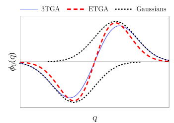
Figure 1: The 3TGA wavepacket is obtained by replacing the extended TGA (ETGA) wavepacket, i.e., a Gaussian multiplied by a linear polynomial, by a sum of two displaced Gaussians (black dotted line).

Let us now describe another generalization of the TGA, which, as the ETGA, can also evaluate the Herzberg–Teller spectra, but, in contrast to the ETGA, can also account for wavepacket splitting. Recall that the ETGA wavepacket is guided by a single trajectory propagated using the local harmonic approximation of the potential at the center of the wavepacket. Whereas the center of a Gaussian maximizes the probability density, this is false for purely Herzberg–Teller wavepackets [Eq. (30) with $\mu_{21}(q_{0})=0$], where the probability density at the center is zero. Although the ETGA is still an exact solution of the time-dependent Schrödinger equation in a global harmonic potential, its performance in a general potential can, therefore, be questioned Lee and Heller (1982). To further investigate the errors introduced by the local harmonic approximation, we propose to approximate the Herzberg–Teller part

$$\phi_{0}^{\text{ETGA-HT}}(q)=\text{$\partial_{q}\mu_{21}$}^{T}\cdot(q-q_{0})\,g_{q_{0}}(q)\,$$ (32)

of the initial state used in the ETGA with an antisymmetric linear combination of two displaced Gaussians (see Fig. 1):

$$\phi_{0}^{\text{3TGA-HT}}(q)=f_{d}\,\left[g_{q_{0}+\Delta_{d}}(q)-g_{q_{0}-\Delta_{d}}(q)\right]\,,$$ (33)

where $g_{q_{c}}(q)$ is a normalized Gaussian $\psi_{0}(q)$ centered at $q_{c}$ instead of $q_{0}$, with zero initial momentum and phase ($p_{0}=\gamma_{0}=0$):

$$g_{q_{c}}(q):=N_{0}\,\,e^{-(q-q_{c})^{T}\cdot A_{0}\cdot(q-q_{c})}\,,$$ (34)

$\Delta_{d}$ is a displacement vector and $f_{d}$ a scaling factor. Note also that the same width matrix $A_{0}$ is used for $g_{q_{c}}$ as for $\psi_{0}(q)$.

We will now show that the approximative wavepacket $\phi_{0}^{\text{3TGA-HT}}$ converges to the exact Herzberg–Teller wavepacket $\phi_{0}^{\text{ETGA-HT}}$when the displacement $\Delta_{d}$ approaches zero along an appropriate direction and a corresponding scaling factor $f_{d}$ is used. For brevity, throughout this subsection we shall again write $\mu$ instead of $\vec{\mu}_{21}(q_{0})\cdot\vec{\epsilon}$ and $\partial_{q}\mu$ instead of $\partial_{q}(\vec{\mu}_{21}(q)\cdot\vec{\epsilon})|_{q_{0}}$.

First, let us discuss the shape of the exact wavepacket $\phi_{0}^{\text{ETGA-HT}}$. Obviously, in one nuclear dimension, $\phi_{0}^{\text{ETGA-HT}}$ has exactly two local extrema: a minimum and a maximum. In Appendix E we prove that this property holds for any number $D$ of nuclear degrees of freedom: there are two and only two local extrema, a maximum and minimum, located at

$$q_{\text{max, min}}^{\text{ETGA-HT}}=q_{0}\pm\Delta q\,,$$ (35)

with the displacement vector

$$\Delta q=\frac{A_{0}^{-1}\cdot\partial_{q}\mu}{\sqrt{2\partial_{q}\mu^{T}\cdot A_{0}^{-1}\cdot\partial_{q}\mu}}.$$ (36)

It is rather obvious that in order for $\phi_{0}^{\text{3TGA-HT}}$ to be a good fit of $\phi_{0}^{\text{ETGA-HT}}$, the two Gaussians in Eq. (33) must be displaced from $q_{0}$ along the direction of the extrema of $\phi_{0}^{\text{ETGA-HT}}$. We therefore choose

$$\Delta_{d}=d\,\Delta q,$$ (37)

where the dimensionless parameter $d$ controls the magnitude of the displacement. The scaling factor $f_{d}$ is obtained by equating the norms of $\phi_{0}^{\text{3TGA-HT}}$ and $\phi_{0}^{\text{ETGA-HT}}$, which gives

$$f_{d}=\frac{\sqrt{2}}{4}\sqrt{\frac{\partial_{q}\mu^{T}\cdot A_{0}^{-1}\cdot\partial_{q}\mu}{1-e^{-d^{2}}}}.$$ (38)

A quick inspection reveals $\phi_{0}^{\text{ETGA-HT}}$ to be a directional derivative of $g_{q_{0}}(q)$ and $\phi_{0}^{\text{3TGA-HT}}$ a finite-difference approximation of this derivative, exact in the limit $d\rightarrow 0$. One can see this explicitly by noting that the normalized initial overlap of the two wavepackets,

$$\frac{\langle\phi_{0}^{\text{ETGA-HT}}|\phi_{0}^{\text{3TGA-HT}}\rangle}{\lVert\phi_{0}^{\text{ETGA-HT}}\rVert^{2}}=\frac{d\,e^{-d^{2}/4}}{\sqrt{1-e^{-d^{2}}}},$$ (39)

is maximized and converges to unity as $d$ approaches zero. Either proof implies that a better description of the initial wavepacket is obtained with smaller values of $d$. On the other hand, anharmonicity effects are included only when the two initial wavepackets are significantly displaced, implying that a larger $d$ is needed. A natural displacement that is neither too small nor too large corresponds to placing the two Gaussians at the extrema of the wavepacket by setting $d=1$ and $\Delta_{d}=\Delta q$; in this case, the initial overlap Eq. (39) is $\approx 98\%$. As this choice of $d$ results in a large initial overlap and in trajectories that correspond to the maxima of the probability density of the Herzberg–Teller component, we recommend using $d=1$ in all applications. However, in the calculations presented in Section IV, we will test not only $d=1$ but also several smaller displacements, giving even larger initial overlaps.

Finally, by adding the Condon term, one obtains a superposition of three Gaussian wavepackets that are propagated independently; the total initial wavepacket in the “three thawed Gaussians approximation” (3TGA) is

$$\phi_{0}^{\text{3TGA}}(q)=\mu\,g_{q_{0}}(q)+f_{d}\,\left[g_{q_{0}+\Delta_{d}}(q)-g_{q_{0}-\Delta_{d}}(q)\right]\,.$$ (40)

In contrast to both the original and extended TGA, where the evolution given by the time-dependent effective Hamiltonian is exactly unitary, the norm of the 3TGA wavepacket is not conserved; since the three Gaussians are propagated with three different effective Hamiltonians, their overlaps are time-dependent and change the norm of the total 3TGA wavepacket. To see this, consider several wavepackets $|\psi_{i}\rangle$, each propagated with its own evolution operator $\hat{U}_{i}$. If $\hat{U}_{i}\neq\hat{U}_{j}$, then the overlap of two such wavepackets is time-dependent:

$$\langle\psi_{i}(t)|\psi_{j}(t)\rangle=\langle\psi_{i}(0)|\hat{U}_{i}^{\dagger}\hat{U}_{j}|\psi_{j}(0)\rangle\neq\langle\psi_{i}(0)|\psi_{j}(0)\rangle\,.$$ (41)

The time dependence of the norm of the 3TGA wavepacket arises from these time-dependent overlaps since

$$\left\|\phi^{\text{3TGA}}(t)\right\|^{2} =\langle\phi^{\text{3TGA}}(t)|\phi^{\text{3TGA}}(t)\rangle$$

$$=\mu^{2}+2f_{d}^{2}\left[1-\text{Re}\left(\langle g_{q_{0}+\Delta_{d}}^{t}|g_{q_{0}-\Delta_{d}}^{t}\rangle\right)\right]$$

$$+2\mu f_{d}\left[\text{Re}\left(\langle g_{q_{0}}^{t}|g_{q_{0}+\Delta_{d}}^{t}\rangle\right)-\text{Re}\left(\langle g_{q_{0}}^{t}|g_{q_{0}-\Delta_{d}}^{t}\rangle\right)\right]\,.$$ (42)

Due to the time dependence of the norm, the calculated dipole time autocorrelation function has to be renormalized at each time step.

II.7 Ab initio implementation

The ab initio implementation of the thawed Gaussian approximation has been discussed in Refs. 29; 30; only a brief overview is given here. The propagation of a thawed Gaussian wavepacket requires a single classical trajectory on the excited-state potential energy surface and the Hessians of the excited-state potential along this trajectory. These data are evaluated in Cartesian coordinates and are then transformed to mass-scaled normal mode coordinates, after removing the translational degrees of freedom by translation to the center of mass frame and rotational degrees of freedom by rotation to the Eckart frame. The choice of the coordinates and correct coordinate transformation is the essence of the on-the-fly ab initio implementation; mass-scaled normal modes of the ground electronic state are useful not only for a straightforward construction of the initial wavepacket, but also for further interpretation of the results.

Within the 3TGA, each thawed Gaussian is propagated using the above mentioned scheme. The initial positions are obtained in the following way: First, the gradient of the transition dipole moment in Cartesian coordinates is projected onto one of three orthogonal polarizations of the electric field and transformed to the ground-state normal mode coordinates. Then the centers of the displaced Gaussians are found and transformed back to Cartesian coordinates for an on-the-fly ab initio propagation. In addition to the central trajectory, each polarization of the electric field requires, in general, two different displaced trajectories to be evaluated.

III Computational details

All ab initio calculations were performed using B3LYP/6-31+G(d,p) density functional theory for the ground state and time-dependent density functional theory for the excited state, as implemented in the Gaussian09 package Frisch et al. . The gradient of the transition dipole moment was computed using a finite-difference approach, as reported in Ref. 32. The ground-state potential energy surface was approximated with a global harmonic potential in order to obtain the initial vibrational state.

The orientational averaging of the 3TGA spectra requires additional trajectories because the gradient of the transition dipole moment depends on the orientation of the molecule. In general, one has to compute the spectrum for three orthogonal orientations of the molecule with respect to the electric field, which implies one central trajectory for the Condon contribution and two additional trajectories for each orientation to represent the Herzberg–Teller contribution to the wavepacket; seven trajectories in total. In phenyl radical, all seven trajectories have to be evaluated, while in benzene, since the transition is symmetry-forbidden and since the gradient of the $z$ component of the transition dipole moment is zero, only four trajectories are needed (two for $x$ and two for $y$ polarization). In contrast, the orientational averaging of the ETGA spectra requires only a single ab initio trajectory because the averaging can be performed by changing only the polynomial part of the wavepacket, which depends on the polarization of the electric field, but does not need additional ab initio data.

A time step of 8 a.u. ($\approx 0.194$ fs) was chosen for all trajectories; 3000 steps (giving a total time of 580 fs) were run for the phenyl radical and 5000 steps (970 fs) for benzene. The Hessians of the potential were computed every four steps, while the intermediate Hessians were obtained by second-order interpolation.

Gaussian broadening of the resulting spectra was used for the phenyl radical (half-width at half-maximum of 100 cm^-1), while for benzene the autocorrelation function is multiplied by $\cos^{2}(\pi t/2T)$ ($T$ is the length of the simulation) because this function preserves most of the autocorrelation function and introduces only slight broadening. However, longer propagation would be required to simulate the spectrum with peaks as narrow as in the experiment. For comparison with experiment, unless otherwise stated, we scale and shift the absorption spectra according to the highest peak: for phenyl radical, all spectra are shifted by $-437$ cm^-1, whereas for benzene we introduce different shifts for the on-the-fly ($3010$ cm^-1), adiabatic harmonic ($3020$ cm^-1), and vertical harmonic spectra ($3300$ cm^-1).

IV Results and discussion

IV.1 Absorption spectrum of the phenyl radical

The absorption spectrum of the $\tilde{\text{A}}^{2}\text{B}_{1}\leftarrow\tilde{\text{X}}^{2}\text{A}_{1}$ electronic transition of the phenyl radical has been a subject of theoretical investigation Kim, Mebel, and Lin (2002); Biczysko, Bloino, and Barone (2009); Baiardi, Bloino, and Barone (2013); Patoz, Begušić, and Vaníček (2018) due to a rich vibronic structure originating from the differences between the ground- and excited-state potential energy surfaces. Whereas the adiabatic harmonic approach, in which the potential is expanded about the excited-state minimum, describes the main features of the absorption spectrum, the vertical harmonic model, which expands the potential about the ground-state minimum, fails completely, as shown in our previous work Patoz, Begušić, and Vaníček (2018). Here we compute the phenyl radical absorption spectrum with the on-the-fly ab initio 3TGA with different values of the displacement parameter $d$ and compare the results to the extended TGA spectrum. Since the anharmonicity of the excited-state potential of the phenyl radical is shown to influence the spectrum more than the Herzberg–Teller contribution Patoz, Begušić, and Vaníček (2018), this system is suited for further investigation using the 3TGA, which is specifically intended for treating the anharmonicity of the Herzberg–Teller active modes. The Herzberg–Teller component of the wavepacket has a larger spread in position than does the Condon component, and therefore is more likely to be influenced strongly by the anharmonicity of the potential. Nevertheless, the calculated 3TGA spectra (see Fig. 2) based on $7$ independent trajectories overlap almost perfectly with the ETGA result based on a single trajectory.

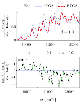
Figure 2: Orientationally averaged absorption spectra of the phenyl radical calculated with the 3TGA (using the default value $d=1$ of the displacement parameter) is compared with the ETGA and experimental Radziszewski (1999) spectra in the top panel, and with the 3TGA spectra using smaller values of the displacement parameter ($d=0.1$ and $d=0.01$) in the bottom panel. Since the 3TGA spectra mostly overlap, the bottom panel shows the scaled difference from the result for $d=1$.

This is somewhat surprising considering that several Herzberg–Teller modes are also displaced and, therefore, experience significant anharmonicity of the potential. The results imply that the local harmonic approximation around the true center of the wavepacket is valid despite the additional spread and the change in the shape of the wavepacket. Interestingly, the spectra evaluated with the 3TGA show almost no dependence on the choice of the initial displacement parameter $d$. This is encouraging since a strong dependence would render the 3TGA method impractical; the fact that the dependence is not only weak but almost nonexistent confirms the results of the single-trajectory ETGA in the phenyl radical.

IV.2 Absorption spectrum of benzene

The symmetry-forbidden $\text{B}_{2\text{u}}\leftarrow\text{A}_{1\text{g}}$ transition of benzene provides a beautiful example of a Herzberg–Teller spectrum that is mentioned in many textbooks due to its simple qualitative interpretation Herzberg (1966); Hollas (2004); Quack and Merkt (2011); Bernath (2005). The experimental and theoretical work on the first excited electronic state of benzene Sobolewski and Domcke (1991); Sobolewski, Woywod, and Domcke (1993) and on the vibronic structure of the corresponding electronic spectrum is so extensive that we can only refer to a small fraction here Sponer et al. (1939); Atkinson and Parmenter (1978); Fischer and Jakobson (1979); Faulkner and Richardson (1979); Fischer and Knight (1992); Trost, Stutz, and Platt (1997); Etzkorn et al. (1999); Bernhardsson et al. (2000); He and Pollak (2001); Borges et al. (2003); Schmied et al. (2004); Worth (2007); Loginov, Braun, and Drabbels (2008); Fally, Carleer, and Vandaele (2009); Penfold and Worth (2009); Li et al. (2010); Crespo-Otero and Barbatti (2012). The main progression corresponds to a totally symmetric ring-breathing vibration Herzberg (1966). Although this transition is forbidden by symmetry, its observation in the absorption spectrum is attributed to the non-totally symmetric vibrations which transform as the $e_{2g}$ irreducible representation. Li et al. Li et al. (2010) include the undisplaced distorted modes in the calculation of the absorption spectrum using a global harmonic model without Duschinsky rotation, i.e., by assuming that the ground- and excited-state normal modes are the same. To go beyond the global harmonic model, Penfold and Worth Worth (2007); Penfold and Worth (2009) combine the construction of an anharmonic potential with the multiconfigurational time-dependent Hartree wavepacket dynamics, producing excellent results, but at the cost of a rather detailed inspection of the system required for reducing the computational cost.

Recently, the on-the-fly ab initio ETGA method has been applied to evaluate the absorption spectrum of benzene with rather high accuracy Patoz, Begušić, and Vaníček (2018). As explained above, this method is an automated, simple to use single-trajectory method, and the fact that the ETGA was much more accurate than both vertical and adiabatic global harmonic models is encouraging. Analogous results for the 3TGA are, therefore, presented in Fig. 3, which compares the on-the-fly ab initio result with the global harmonic spectra (top panel). Note that the failure of the vertical harmonic model in the phenyl radical and benzene is not a rule—there are many cases, such as the absorption and photoelectron spectra of ammonia Domcke et al. (1977); Wehrle, Šulc, and Vaníček (2014); Wehrle, Oberli, and Vaníček (2015), in which the vertical is more accurate than the adiabatic harmonic model. Indeed, the vertical harmonic model describes the Franck-Condon region better and so might be expected to be a good model for vertical transitions. The on-the-fly ab initio approach, however, overcomes the issue of choosing the geometry for expanding the potential and is expected to be always at least as good as the better of the two global harmonic models. Moreover, as Fig. 3 shows, the inclusion of anharmonicity in benzene is essential for obtaining a quantitative agreement—compare the 3TGA with the adiabatic harmonic model, which is at least qualitatively correct here.

Finally, the bottom panel of Fig. 3 demonstrates that in benzene the Herzberg–Teller term, captured with the 3TGA, is responsible for the observation of the spectrum because the Condon approximation yields a zero spectrum. This is, indeed, one of the main reasons why we have implemented the 3TGA; the original TGA is often sufficient for Condon spectra.

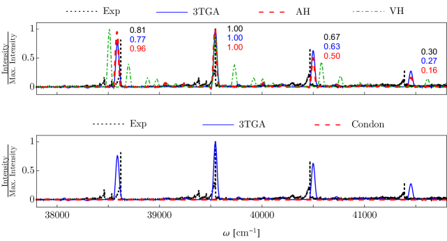
Figure 3: Orientationally averaged absorption spectrum of benzene calculated with the 3TGA (with $d=1$) is compared with the experimental Fally, Carleer, and Vandaele (2009); Keller-Rudek et al. (2013) and global harmonic spectra computed using the adiabatic harmonic (AH) and vertical harmonic (VH) models (top panel). In the bottom panel the full Herzberg–Teller spectrum computed with the 3TGA is compared to the purely Condon spectrum, which is exactly zero due to symmetry of benzene, but which could be computed with the original TGA using a single thawed Gaussian.

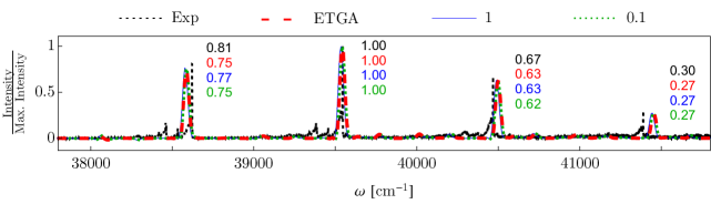
Figure 4: Orientationally averaged absorption spectra of benzene calculated with the 3TGA for a larger ($d=1$) and smaller ($d=0.1$) displacements are compared with the ETGA and experimental Fally, Carleer, and Vandaele (2009); Keller-Rudek et al. (2013) spectra.

To investigate the importance of anharmonicity in more detail, the spectra calculated with the 3TGA and ETGA are compared in Fig. 4. Whereas the 3TGA method with the smaller displacement parameter $d$ gives almost the same result as the ETGA approach, the 3TGA spectrum calculated with $d=1$ is red-shifted by $\approx 10$ cm^-1 and the intensity of the first stronger peak is slightly improved. Due to symmetry, the Herzberg–Teller modes cannot be displaced from the minimum, so they do not contribute significantly to the shape of the spectrum. Nevertheless, these modes can influence the total energy shift of the spectrum, which is in accord with the observed results.

IV.3 Norm conservation and fidelity

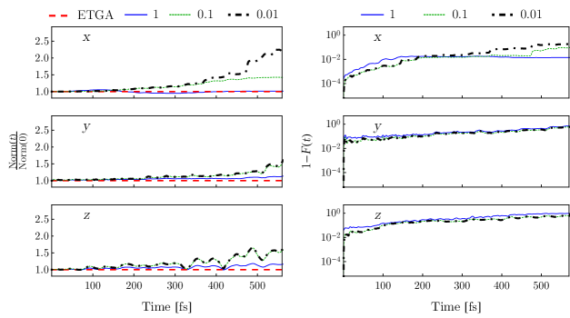
Figure 5: Norm (left panels) of the ETGA and 3TGA wavepackets, and fidelity (right panels) between the ETGA and 3TGA wavepackets [see Eq. (43)] for the phenyl radical. Results for three different values of the displacement parameter ($d=0.01$, $0.1$, and $1$) as well as for all three different polarizations ($x$, $y$, and $z$) of the electric field are presented.

In contrast with the single-trajectory ETGA, the norm of the 3TGA wavepacket is not conserved because the 3TGA wavepacket is a superposition of wavepackets, each of which feels its own time-dependent potential. Indeed, the numerical results for the phenyl radical (see Fig. 5) and benzene (see Fig. 6) confirm this theoretical prediction from Subsection II.6. Interestingly, larger displacement ($d=1$) , which corresponds to placing the additional Gaussians at the extrema of the initial wavepacket, gives smaller deviations of the norm from unity. In Eq. (42) the time-dependent terms are multiplied by the scaling factor $f_{d}$, indicating that the norm should vary more for smaller displacements, since the factor $f_{d}$ decreases with the displacement. This is in contrast with the expectation that the wavepacket propagation, including the conservation of the norm, should converge to the ETGA with smaller displacements. The fidelity between the 3TGA and ETGA wavepackets,

$$F(t):=\frac{|\langle\phi^{\text{ETGA}}(t)|\psi^{\text{3TGA}}(t)\rangle|^{2}}{||\psi^{\text{ETGA}}(t)||^{2}\,||\psi^{\text{3TGA}}(t)||^{2}}=\frac{|\langle\phi^{\text{ETGA}}(t)|\psi^{\text{3TGA}}(t)\rangle|^{2}}{||\psi^{\text{3TGA}}(t)||^{2}}\,,$$ (43)

can be used as a measure for comparing the quantum dynamics obtained with the two semiclassical approximations; it shows deviations of the three thawed Gaussians from the extended thawed Gaussian wavepacket propagated on the excited-state potential energy surface. As can be seen in Figs. 5 and 6, the fidelity decays similarly for all values of the displacement parameter, despite the differences in the initial overlaps. Although the fidelity decays quickly over time, the final spectra evaluated with the two approximations are nearly the same.

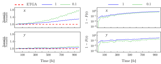
Figure 6: Norm (left panels) of the ETGA and 3TGA wavepackets, and the fidelity (right panels) between the ETGA and 3TGA wavepackets [see Eq. (43)] for benzene. Results for two different values of the displacement parameter ($d=0.1$ and $1$) and two different polarizations ($x$ and $y$) of the electric field are presented. Results for the $z$ polarization are not shown because the corresponding components of the transition dipole moment and its gradient are zero.

V Conclusion

We have presented the 3TGA, constructed by replacing the Herzberg–Teller part of the initial wavepacket with two displaced Gaussians, in order to describe electronic spectra beyond the Condon approximation and anharmonicity effects beyond the single-trajectory ETGA.

The 3TGA presented here is still a very rough approximation to the exact nuclear wavepacket dynamics. Nevertheless, compared to the global harmonic models, which are frequently employed in computational chemistry, the on-the-fly ab initio methods based on the TGA offer a rather computationally cheap way to partially include anharmonicity. Moreover, the 3TGA allows us to analyze the validity of the single-trajectory ETGA; our results confirm that the additional spread of the wavepacket, induced by the Herzberg–Teller contribution, does not lead to a significant wavepacket splitting during the dynamics induced by electronic absorption in the phenyl radical and benzene.

To conclude, the on-the-fly ab initio implementation of the 3TGA is capable of describing anharmonicity effects and Herzberg–Teller contribution to the spectra, as well as of evaluating both symmetry-forbidden and weakly allowed spectra. The extension beyond the single-trajectory ETGA approach suggests the viability of simple semiclassical methods that can include wavepacket splitting and associated interference, and which would readily outperform global harmonic and single-trajectory methods, while remaining computationally feasible compared to the more advanced semiclassical and quantum methods. Indeed, a related pragmatic approach of using a small number of well-defined, rather than sampled initial conditions, was employed in the multiple coherent states time-averaged semiclassical initial value representation (MC-TA-SC-IVR) Gabas, Conte, and Ceotto (2017) and its “divide-and-conquer” extension Ceotto, Di Liberto, and Conte (2017), which were used to evaluate positions of peaks in vibrational spectra with rather high accuracy. Another appealing feature of the 3TGA is that, despite its simplicity, the resulting spectrum contains the information not only about the positions but also about the intensities of the peaks; this is because the initial conditions are determined by the shape of the initial wavepacket. Last but not least, like MC-TA-SC-IVR, but in contrast to some semiclassical methods that require tens of thousands of trajectories for convergence, the 3TGA, by using only three uniquely defined trajectories (we recommend using $d=1$ always) does not destroy the appealing intuitive picture provided by the original or extended TGA based on a single trajectory. As a result, we anticipate further development of efficient methods using only a few trajectories for semiclassical propagation.

Appendix A Orientational average

Let $\overleftrightarrow{T}$ be a second-order tensor in $3$ dimensions (i.e., a $3\times 3$ matrix) and let us evaluate the average of the scalar

$$T(\vec{\epsilon}):=\vec{\epsilon}^{T}\cdot\overleftrightarrow{T}\cdot\vec{\epsilon}$$ (44)

over all unit vectors $\vec{\epsilon}$, i.e.,

$$\overline{T(\vec{\epsilon})}:=\frac{1}{4\pi}\int_{S^{2}}T(\vec{\epsilon})d\Omega.$$ (45)

($\int_{S^{2}}\cdots d\Omega$ denotes the integration over the two-dimensional unit sphere $S^{2}$.) We shall prove that the result of this average is simply one third of the trace of the tensor:

$$\overline{T(\vec{\epsilon})}=\frac{1}{3}\operatorname*{Tr}\overleftrightarrow{T}.$$ (46)

In particular, in Cartesian coordinates,

$$\overline{T(\vec{\epsilon})}=\frac{1}{3}(T_{xx}+T_{yy}+T_{zz}).$$ (47)

Proof: In polar coordinates $(\theta,\varphi)$, the unit vector $\vec{\epsilon}$ is expressed as

$$\vec{\epsilon}=\left(\sin{\theta}\cos{\varphi},\ \sin{\theta}\sin{\varphi},\ \cos{\theta}\right).$$ (48)

Using Eq. (48), scalar (44) becomes

$$T(\vec{\epsilon}) =\left(T_{xx}\cos^{2}\varphi+T_{yy}\sin^{2}\varphi\right)\sin^{2}\theta+T_{zz}\cos^{2}\theta$$

$$+\left(T_{xy}+T_{yx}\right)\sin^{2}\theta\sin\varphi\cos\varphi+\cdots,$$

where $\cdots$ denote additional, analogous cross terms for $T_{xz}+T_{zx}$ and $T_{yz}+T_{zy}$. The integration over the unit sphere,

$$\overline{T(\vec{\epsilon})}=\frac{1}{4\pi}\int_{0}^{\pi}d\theta\sin\theta\int_{0}^{2\pi}d\varphi\,T(\vec{\epsilon}),$$

suppresses all the cross terms; e.g., $\sin\varphi\cos\varphi=(1/2)\sin\left(2\varphi\right)$ and the integration over $\varphi$ of the cross term for $T_{xy}+T_{yx}$ is, therefore, zero. Integration of the diagonal terms over $\varphi$ and making a substitution $u:=\cos\theta$ gives

$$\overline{T(\vec{\epsilon})} =\frac{1}{4}\int_{-1}^{1}du\left[\left(T_{xx}+T_{yy}\right)(1-u^{2})+2T_{zz}u^{2}\right]$$

$$=\frac{1}{4}\left[\left(T_{xx}+T_{yy}\right)(u-u^{3}/3)+2T_{zz}u^{3}/3\right]_{-1}^{1}$$

$$=\frac{1}{3}\left(T_{xx}+T_{yy}+T_{zz}\right)=\frac{1}{3}\operatorname*{Tr}\overleftrightarrow{T},$$

where in the last step we used the invariance of the trace of a tensor under coordinate transformations, in order to obtain the coordinate-independent expression (46).

Appendix B Proof of the expression (11) for the gradient of the transition dipole moment

Before it is expressed in the basis of electronic states, the molecular electric dipole operator is simply a sum

$$\hat{\vec{\mu}}_{\text{mol}}\equiv\vec{\mu}_{\text{mol}}(q,\{\hat{\vec{r}}_{n}\})=\vec{\mu}_{\text{nu}}(q)+\vec{\mu}_{\text{el}}(\{\hat{\vec{r}}_{n}\})$$

of its nuclear component $\vec{\mu}_{\text{nu}}(q)$ given in Eq. (14) and electronic component

$$\vec{\mu}_{\text{el}}(\{\hat{\vec{r}}_{n}\})=-e\sum_{n=1}^{N_{\text{el}}}\hat{\vec{r}}_{n},$$ (49)

where $\vec{r}_{n}$ are the Cartesian coordinates of the $n$th electron and $\{\vec{r}_{n}\}:=(\vec{r}_{1},\ldots,\vec{r}_{N_{\text{el}}})$. Relation (11) is proven directly by taking the gradient of Eq. (12):

$$\partial_{j}\vec{\mu}_{\alpha\beta}(q) =\langle\partial_{j}\alpha|\hat{\vec{\mu}}_{\text{mol}}|\beta\rangle+\langle\alpha|\hat{\vec{\mu}}_{\text{mol}}|\partial_{j}\beta\rangle+\langle\alpha|\partial_{j}\hat{\vec{\mu}}_{\text{mol}}|\beta\rangle$$ (50)

$$=\sum_{\gamma}\left(\langle\partial_{j}\alpha|\gamma\rangle\langle\gamma|\hat{\vec{\mu}}_{\text{mol}}|\beta\rangle+\langle\alpha|\hat{\vec{\mu}}_{\text{mol}}|\gamma\rangle\langle\gamma|\partial_{j}\beta\rangle\right)+\langle\alpha|\partial_{j}\vec{\mu}_{\text{nu}}(q)|\beta\rangle$$ (51)

$$=\sum_{\gamma}\left(F_{\alpha\gamma,j}^{{\dagger}}\vec{\mu}_{\gamma\beta}+\vec{\mu}_{\alpha\gamma}F_{\gamma\beta,j}\right)+\partial_{j}\vec{\mu}_{\text{nu}}(q)\delta_{\alpha\beta}$$ (52)

$$=\sum_{\gamma}\left(-F_{\alpha\gamma,j}\vec{\mu}_{\gamma\beta}+\vec{\mu}_{\alpha\gamma}F_{\gamma\beta,j}\right)+\partial_{j}\vec{\mu}_{\text{nu}}(q)\delta_{\alpha\beta}$$ (53)

$$=\left[\vec{\bm{\mu}},\mathbf{F}_{j}\right]_{\alpha\beta}+\partial_{j}\vec{\mu}_{\text{nu}}(q)\delta_{\alpha\beta}.$$ (54)

The first equality follows from the Leibniz law; the second equality employs a resolution of identity over electronic states and takes into account that the electronic dipole moment operator (49) is independent of nuclear coordinates; the third equality follows from the definition (13) of nonadiabatic coupling vectors, the fact that $\partial_{j}\vec{\mu}_{\text{nu}}(q)$ is a purely nuclear operator, and orthogonality of the electronic states; the fourth equality uses the antihermitian property of the matrix of nonadiabatic couplings,

$$\mathbf{F}_{j}^{{\dagger}}=-\mathbf{F}_{j},$$

which follows from the orthogonality of the electronic states,

$$0=\partial_{j}\delta_{\alpha\beta}=\partial_{j}\langle\alpha(q)|\beta(q)\rangle=F_{\alpha\beta,j}^{{\dagger}}+F_{\alpha\beta,j};$$

the fifth step completes the proof.

Appendix C Propagation of the width and phase of the thawed Gaussian wavepacket

The approach by Lee and Heller Lee and Heller (1982) suggests splitting the complex symmetric width matrix $A$ into a product of two matrices $P$ and $Z$:

$$A_{t}=-\frac{i}{2\hbar}P_{t}\cdot Z_{t}^{-1}\,.$$ (55)

By imposing $\dot{Z}_{t}=m^{-1}\cdot P_{t}$, with the initial conditions $Z_{0}=I$, where $I$ is the identity matrix, and $P_{0}=2i\hbar A_{0}$, the expression for the propagation of $Z$ and $P$ parameters is obtained:

$$\begin{pmatrix}Z_{t}\\ P_{t}\end{pmatrix}=M_{t}\begin{pmatrix}Z_{0}\\ P_{0}\end{pmatrix}\,.$$ (56)

Regarding $\gamma_{t}$, which is a generalization of classical action and represents both the dynamical phase and normalization, it is evaluated as

$$\gamma_{t} =\gamma_{0}+\int_{0}^{t}L_{\tau}d\tau-\hbar^{2}\int_{0}^{t}\operatorname{Tr}\left(m^{-1}\cdot A_{\tau}\right)d\tau$$ (57)

$$=\gamma_{0}+\int_{0}^{t}L_{\tau}d\tau-\hbar^{2}\int_{0}^{t}\operatorname{Tr}\left(-\frac{i}{2\hbar}\dot{Z}_{\tau}\cdot Z_{\tau}^{-1}\right)d\tau$$ (58)

$$=\gamma_{0}+\int_{0}^{t}L_{\tau}d\tau+\frac{i\hbar}{2}\ln\left(\det Z_{t}\right)\,,$$ (59)

where the conditions imposed on $Z$ and $P$ are used in order to obtain the final expression. Note that, since the determinant in the final expression is complex, a proper branch of the logarithm has to be taken in order to make $\gamma_{t}$ continuous in time. If continuity were not imposed on $\gamma_{t}$, the wavepacket would show sudden jumps by $\pi$ in the overall phase. Phase continuity is also important in the evaluation of the correlation function, which comprises a square root of a complex determinant $\det(A_{0}+A_{t}^{\ast})$. The continuity of the correlation function is enforced by taking the appropriate branch of the square root.

Appendix D Derivation of the extended thawed Gaussian approximation

Proof of Eq. (29): The effective potential (21) depends on $t$ only implicitly, via $q_{t}$. Considering $V_{\text{eff}}$ as a function of $q$ and $q_{t}$, its dependence on $q_{t}$ is

$$\frac{\partial V_{\text{eff}}(q,q_{t})}{\partial q_{t}}=\frac{1}{2}V^{\prime\prime\prime}|_{q_{t}}\left(q-q_{t},q-q_{t},\cdot\right)$$ (60)

because in the derivation of Eq. (60) the sum $\partial_{q}V|_{q_{t}}+\operatorname{Hess}_{q}V|_{q_{t}}\cdot(q-q_{t})$ appears twice, with opposite signs, and therefore cancels. [Here $V^{\prime\prime\prime}$ is a rank-$3$ tensor of the third derivatives of $V$ and the dot $\cdot$ in the third argument of $V^{\prime\prime\prime}$ indicates that the tensor has been only partially contracted; the right-hand side of Eq. (60) is still a vector.] Within local harmonic approximation (LHA), where all derivatives of $V$ at $q_{t}$ beyond the second are neglected,

$$\frac{\partial V_{\text{eff}}}{\partial q_{t}}\overset{\text{LHA}}{=}0\text{.}$$ (61)

Equation (61) implies that the effective Hamiltonian operator (20), considered as a function of initial conditions $q_{0}$ and $p_{0}$, $\hat{H}_{\text{eff}}(q_{0},p_{0},t)\equiv H_{\text{eff}}(\hat{q},\hat{p},q_{0},p_{0},t)$, is independent of $p_{0}$:

$$\frac{\partial\hat{H}_{\text{eff}}}{\partial p_{0}}=\left(\frac{\partial q_{t}}{\partial p_{0}}\right)^{T}\cdot\frac{\partial\hat{V}_{\text{eff}}}{\partial q_{t}}\overset{\text{LHA}}{=}0\text{.}$$ (62)

The effective time evolution operator

$$\hat{U}(q_{0},p_{0},t):=\mathcal{T}\exp\left[-\frac{i}{\hbar}\int_{0}^{t}\hat{H}_{\text{eff}}(q_{0},p_{0},\tau)d\tau\right]$$

induced by $\hat{H}_{\text{eff}}$ is, in general, a function of $q_{0}$ and $p_{0}$, but factorizing the time-ordered product into a product of exponentials for infinitesimal time steps, expanding the exponential for each time step into a Taylor series, and using Eq. (62) shows that, within the LHA,

$$\frac{\partial\hat{U}(q_{0},p_{0},t)}{\partial p_{0}}\overset{\text{LHA}}{=}0$$ (63)

and, indeed, any polynomial in derivatives with respect to $p_{0}$ acting on $\hat{U}$ vanishes:

$$P\left(\frac{\hbar}{i}\frac{\partial}{\partial p_{0}}\right)\hat{U}(q_{0},p_{0},t)\overset{\text{LHA}}{=}0.$$ (64)

The initial Herzberg-Teller state $|\phi_{0}\rangle$ propagated to time $t$ is

$$|\phi_{t}\rangle =\hat{U}(q_{0},p_{0},t)|\phi_{0}\rangle=\hat{U}(q_{0},p_{0},t)P\left(\frac{\hbar}{i}\frac{\partial}{\partial p_{0}}\right)|\psi_{0}\rangle$$

$$=P\left(\frac{\hbar}{i}\frac{\partial}{\partial p_{0}}\right)\hat{U}(q_{0},p_{0},t)|\psi_{0}\rangle=P\left(\frac{\hbar}{i}\frac{\partial}{\partial p_{0}}\right)|\psi_{t}\rangle,$$ (65)

where the Dirac kets $|\psi_{0}\rangle$ and $|\psi_{t}\rangle$ are considered as functions of $q_{0}$ and $p_{0},$ and Eq. (64) was used to switch the order of $P$ and $\hat{U}$. This completes the proof of Eq. (29).

Proof of Eqs. (30) and (31): Let us evaluate the derivative $\partial|\psi_{t}\rangle/\partial p_{0}$, needed in Eq. (65), analytically in position representation, in which $|\psi_{t}\rangle$ is the TGA wavefunction (19):

$$\frac{\partial\psi_{t}(q)}{\partial p_{0}}\overset{\text{LHA}}{=}\left(\frac{\partial q_{t}}{\partial p_{0}}\right)^{T}\cdot\frac{\partial\psi_{t}}{\partial q_{t}}+\left(\frac{\partial p_{t}}{\partial p_{0}}\right)^{T}\cdot\frac{\partial\psi_{t}}{\partial p_{t}}+\left(\frac{\partial\gamma_{t}}{\partial p_{0}}\right)^{T}\cdot\frac{\partial\psi_{t}}{\partial\gamma_{t}}$$

$$=\left\{M_{t,qp}^{T}\cdot\left[2A_{t}\cdot\left(q-q_{t}\right)-\frac{i}{\hbar}p_{t}\right]+M_{t,pp}^{T}\cdot\frac{i}{\hbar}\left(q-q_{t}\right)+M_{t,qp}^{T}\cdot p_{t}\frac{i}{\hbar}\right\}\psi_{t}(q),$$

$$=\left(2M_{t,qp}^{T}\cdot A_{t}+\frac{i}{\hbar}M_{t,pp}^{T}\right)\cdot\left(q-q_{t}\right)\psi_{t}(q).$$ (66)

In the first step of the derivation, we neglected the dependence of the width matrix $A_{t}$ on $p_{0}$, which follows from Eq. (24) within the LHA. In the second step, we used the derivative

$$\frac{\partial\gamma_{t}}{\partial p_{0}}=\frac{\partial S_{t}\left(q_{0},p_{0}\right)}{\partial p_{0}}=\left(\frac{\partial q_{t}}{\partial p_{0}}\right)^{T}\cdot\frac{\partial S_{t}\left(q_{0},q_{t}\right)}{\partial q_{t}}=M_{t,qp}^{T}\cdot p_{t},$$

where $S_{t}=\int_{0}^{t}L_{\tau}d\tau$ is the classical action component of $\gamma_{t}$ expressed either as a function of $q_{0}$ and $p_{0}$ or of $q_{0}$ and $q_{t}$. The derivation of the central ETGA equations (30) and (31) is completed by substituting the Herzberg-Teller form [Eq. (10)] of the polynomial $P$,

$$P(x)=\mu_{21}\left(q_{0}\right)+\partial_{q}\mu_{21}|_{q_{0}}^{T}\cdot x,$$

into Eq. (29), giving

$$\phi_{t}(q)=\left[\mu_{21}\left(q_{0}\right)+\partial_{q}\mu_{21}|_{q_{0}}^{T}\cdot\frac{\hbar}{i}\frac{\partial}{\partial p_{0}}\right]\psi_{t}(q),$$

and using expression (66) for $\partial\psi_{t}(q)/\partial p_{0}$.

Appendix E Extrema of the Herzberg–Teller part of the wavepacket

The extrema of the wavepacket (32) are found by setting its gradient to zero. The gradient, given by

$$\partial_{q}\phi_{0}^{\text{ETGA-HT}}(q)=\left[\partial_{q}\mu-2\left(\partial_{q}\mu^{T}\cdot\Delta q\right)A_{0}\cdot\Delta q\right]g_{q_{0}}(q)\,,$$ (67)

where $\Delta q=q-q_{0}$, will be zero if and only if

$$\partial_{q}\mu=2(\partial_{q}\mu^{T}\cdot\Delta q)A_{0}\cdot\Delta q$$ (68)

because the Gaussian function $g_{q_{0}}(q)$ is strictly positive. Since the initial width matrix $A_{0}$ is positive definite, it has an inverse and we can multiply Eq. (68) on the left with $A_{0}^{-1}$, which gives

$$A_{0}^{-1}\cdot\partial_{q}\mu=2(\partial_{q}\mu^{T}\cdot\Delta q)\Delta q$$ (69)

Scalar product of Eq. (69) with the vector $\partial_{q}\mu$ gives

$$\partial_{q}\mu^{T}\cdot A_{0}^{-1}\cdot\partial_{q}\mu=2(\partial_{q}\mu^{T}\cdot\Delta q)^{2},$$ (70)

with two solutions

$$\partial_{q}\mu^{T}\cdot\Delta q=\pm\sqrt{\frac{1}{2}\partial_{q}\mu^{T}\cdot A_{0}^{-1}\cdot\partial_{q}\mu}.$$ (71)

Finally, substitution of $\partial_{q}\mu^{T}\cdot\Delta q$ from Eq. (71) into Eq. (69) yields

$$\Delta q=\pm\frac{\sqrt{2}}{2}\frac{A_{0}^{-1}\cdot\partial_{q}\mu}{\sqrt{\partial_{q}\mu^{T}\cdot A_{0}^{-1}\cdot\partial_{q}\mu}},$$

where it is easy to see that the positive sign corresponds to the local maximum and negative sign to the local minimum, completing the proof of Eqs. (35) and (36).

References

- Quack and Merkt (2011) M. Quack and F. Merkt, Handbook of High-resolution Spectroscopy (John Wiley & Sons, 2011).
- Herzberg (1966) G. Herzberg, Molecular Spectra and Molecular Structure: III. Electronic Spectra of Polyatomic Molecules (D.Van Nostrand Company Inc., 1966).
- Heller (1981a) E. J. Heller, Acc. Chem. Res. 14, 368 (1981a).
- Mukamel (1995) S. S. Mukamel, Principles of nonlinear optical spectroscopy (New York ; Oxford : Oxford University Press, 1995).
- Meyer, Gatti, and Worth (2009) H.-D. Meyer, F. Gatti, and G. A. Worth, Multidimensional Quantum Dynamics: MCTDH Theory and Applications (WILEY-VCH, 2009).
- Gatti (2014) F. Gatti, Molecular Quantum Dynamics - From Theory to Applications (Springer-Verlag, 2014).
- Miller (1970) W. H. Miller, J. Chem. Phys. 53, 3578 (1970).
- Miller (2001) W. H. Miller, J. Phys. Chem. A 105, 2942 (2001).
- Herman and Kluk (1984) M. F. Herman and E. Kluk, Chem. Phys. 91, 27 (1984).
- Kay (2005) K. G. Kay, Annu. Rev. Phys. Chem. 56, 255 (2005).
- Zhang and Pollak (2004) S. Zhang and E. Pollak, J. Chem. Phys. 121, 3384 (2004).
- Grossmann (2006) F. Grossmann, J. Chem. Phys. 125, 014111 (2006).
- Mollica and Vaníček (2011) C. Mollica and J. Vaníček, Phys. Rev. Lett. 107, 214101 (2011).
- Ceotto, Di Liberto, and Conte (2017) M. Ceotto, G. Di Liberto, and R. Conte, Phys. Rev. Lett. 119, 010401 (2017).
- Buchholz, Grossmann, and Ceotto (2018) M. Buchholz, F. Grossmann, and M. Ceotto, J. Chem. Phys. 148, 114107 (2018).
- Heller (1975) E. J. Heller, J. Chem. Phys. 62, 1544 (1975).
- Heller (1981b) E. J. Heller, J. Chem. Phys. 75, 2923 (1981b).
- Ben-Nun, Quenneville, and Martínez (2000) M. Ben-Nun, J. Quenneville, and T. J. Martínez, J. Phys. Chem. A 104, 5161 (2000).
- Saita and Shalashilin (2012) K. Saita and D. V. Shalashilin, J. Chem. Phys. 137, 22A506 (2012).
- Makhov et al. (2017) D. V. Makhov, C. Symonds, S. Fernandez-Alberti, and D. V. Shalashilin, Chem. Phys. 493, 200 (2017).
- Richings et al. (2015) G. Richings, I. Polyak, K. Spinlove, G. Worth, I. Burghardt, and B. Lasorne, Int. Rev. Phys. Chem. 34, 269 (2015).
- Curchod and Martínez (2018) B. F. E. Curchod and T. J. Martínez, Chem. Rev. 118, 3305 (2018).
- Tatchen and Pollak (2009) J. Tatchen and E. Pollak, J. Chem. Phys. 130, 041103 (2009).
- Ceotto et al. (2009a) M. Ceotto, S. Atahan, S. Shim, G. F. Tantardini, and A. Aspuru-Guzik, Phys. Chem. Chem. Phys. 11, 3861 (2009a).
- Ceotto et al. (2009b) M. Ceotto, S. Atahan, G. F. Tantardini, and A. Aspuru-Guzik, J. Chem. Phys. 130, 234113 (2009b).
- Wong et al. (2011) S. Y. Y. Wong, D. M. Benoit, M. Lewerenz, A. Brown, and P.-N. Roy, J. Chem. Phys. 134, 094110 (2011).
- Ianconescu, Tatchen, and Pollak (2013) R. Ianconescu, J. Tatchen, and E. Pollak, J. Chem. Phys. 139, 154311 (2013).
- Gabas, Conte, and Ceotto (2017) F. Gabas, R. Conte, and M. Ceotto, J. Chem. Theory Comput. 13, 2378 (2017).
- Wehrle, Šulc, and Vaníček (2014) M. Wehrle, M. Šulc, and J. Vaníček, J. Chem. Phys. 140, 244114 (2014).
- Wehrle, Oberli, and Vaníček (2015) M. Wehrle, S. Oberli, and J. Vaníček, J. Phys. Chem. A 119, 5685 (2015).
- Mahapatra et al. (2005) S. Mahapatra, V. Vallet, C. Woywod, H. Köppel, and W. Domcke, J. Chem. Phys. 123, 231103 (2005).
- Patoz, Begušić, and Vaníček (2018) A. Patoz, T. Begušić, and J. Vaníček, J. Phys. Chem. Lett. 9, 2367 (2018).
- Lee and Heller (1982) S.-Y. Lee and E. J. Heller, J. Chem. Phys. 76, 3035 (1982).
- Andrews and Thirunamachandran (1977) D. L. Andrews and T. Thirunamachandran, J. Chem. Phys. 67, 5026 (1977).
- Gelin, Borrelli, and Domcke (2017) M. F. Gelin, R. Borrelli, and W. Domcke, J. Chem. Phys. 147, 044114 (2017).
- Hein et al. (2012) B. Hein, C. Kreisbeck, T. Kramer, and M. Rodríguez, New J. Phys. 14, 023018 (2012).
- Condon (1926) E. Condon, Phys. Rev. 28, 1182 (1926).
- Herzberg and Teller (1933) G. Herzberg and E. Teller, Z. Phys. Chem. B 21, 410 (1933).
- Seidner et al. (1992) L. Seidner, G. Stock, A. L. Sobolewski, and W. Domcke, J. Chem. Phys. 96, 5298 (1992).
- Li et al. (2010) J. Li, C.-K. Lin, X. Y. Li, C. Y. Zhu, and S. H. Lin, Phys. Chem. Chem. Phys. 12, 14967 (2010).
- (41) M. J. Frisch, G. W. Trucks, H. B. Schlegel, G. E. Scuseria, M. A. Robb, J. R. Cheeseman, G. Scalmani, V. Barone, B. Mennucci, G. A. Petersson, H. Nakatsuji, M. Caricato, X. Li, H. P. Hratchian, A. F. Izmaylov, J. Bloino, G. Zheng, J. L. Sonnenberg, M. Hada, M. Ehara, K. Toyota, R. Fukuda, J. Hasegawa, M. Ishida, T. Nakajima, Y. Honda, O. Kitao, H. Nakai, T. Vreven, J. A. Montgomery, Jr., J. E. Peralta, F. Ogliaro, M. Bearpark, J. J. Heyd, E. Brothers, K. N. Kudin, V. N. Staroverov, R. Kobayashi, J. Normand, K. Raghavachari, A. Rendell, J. C. Burant, S. S. Iyengar, J. Tomasi, M. Cossi, N. Rega, J. M. Millam, M. Klene, J. E. Knox, J. B. Cross, V. Bakken, C. Adamo, J. Jaramillo, R. Gomperts, R. E. Stratmann, O. Yazyev, A. J. Austin, R. Cammi, C. Pomelli, J. W. Ochterski, R. L. Martin, K. Morokuma, V. G. Zakrzewski, G. A. Voth, P. Salvador, J. J. Dannenberg, S. Dapprich, A. D. Daniels, O. Farkas, J. B. Foresman, J. V. Ortiz, J. Cioslowski, and D. J. Fox, “Gaussian 09 Revision D.01,” Gaussian Inc. Wallingford CT 2009.
- Kim, Mebel, and Lin (2002) G. S. Kim, A. M. Mebel, and S. H. Lin, Chem. Phys. Lett. 361, 421 (2002).
- Biczysko, Bloino, and Barone (2009) M. Biczysko, J. Bloino, and V. Barone, Chem. Phys. Lett. 471, 143 (2009).
- Baiardi, Bloino, and Barone (2013) A. Baiardi, J. Bloino, and V. Barone, J. Chem. Theory Comput. 9, 4097 (2013).
- Radziszewski (1999) J. Radziszewski, Chem. Phys. Lett. 301, 565 (1999).
- Hollas (2004) J. Hollas, Modern Specroscopy, 4th ed. (John Wiley & Sons, Ltd., 2004).
- Bernath (2005) P. F. Bernath, Spectra of atoms and molecules, 2nd ed. (Oxford University Press, 2005).
- Sobolewski and Domcke (1991) A. L. Sobolewski and W. Domcke, Chem. Phys. Lett. 180, 381 (1991).
- Sobolewski, Woywod, and Domcke (1993) A. L. Sobolewski, C. Woywod, and W. Domcke, J. Chem. Phys. 98, 5627 (1993).
- Sponer et al. (1939) H. Sponer, G. Nordheim, A. L. Sklar, and E. Teller, J. Chem. Phys. 7, 207 (1939).
- Atkinson and Parmenter (1978) G. H. Atkinson and C. S. Parmenter, J. Mol. Spec. 73, 20 (1978).
- Fischer and Jakobson (1979) G. Fischer and S. Jakobson, Mol. Phys. 38, 299 (1979).
- Faulkner and Richardson (1979) T. R. Faulkner and F. S. Richardson, J. Chem. Phys. 70, 1201 (1979).
- Fischer and Knight (1992) G. Fischer and A. E. W. Knight, Chem. Phys. 168, 211 (1992).
- Trost, Stutz, and Platt (1997) B. Trost, J. Stutz, and U. Platt, Atmos. Environ. 31, 3999 (1997).
- Etzkorn et al. (1999) T. Etzkorn, B. Klotz, S. Sørensen, I. V. Patroescu, I. Barnes, K. H. Becker, and U. Platt, Atmos. Environ. 33, 525 (1999).
- Bernhardsson et al. (2000) A. Bernhardsson, N. Forsberg, P. Malmqvist, B. O. Roos, and L. Serrano-Andres, J. Chem. Phys. 112, 2798 (2000).
- He and Pollak (2001) Y. He and E. Pollak, J. Phys. Chem. A 105, 10961 (2001).
- Borges et al. (2003) I. Borges, A. J. C. Varandas, A. B. Rocha, and C. E. Bielschowsky, J. Mol. Struct. THEOCHEM 621, 99 (2003).
- Schmied et al. (2004) R. Schmied, P. Çarçabal, A. M. Dokter, V. P. A. Lonij, K. K. Lehmann, and G. Scoles, J. Chem. Phys. 121, 2701 (2004).
- Worth (2007) G. Worth, J. Photoch. Photobio. A 190, 190 (2007).
- Loginov, Braun, and Drabbels (2008) E. Loginov, A. Braun, and M. Drabbels, Phys. Chem. Chem. Phys. 10, 6107 (2008).
- Fally, Carleer, and Vandaele (2009) S. Fally, M. Carleer, and A. C. Vandaele, J. Quant. Spectrosc. Radiat. Transf. 110, 766 (2009).
- Penfold and Worth (2009) T. J. Penfold and G. A. Worth, J. Chem. Phys. 131, 064303 (2009).
- Crespo-Otero and Barbatti (2012) R. Crespo-Otero and M. Barbatti, Theor. Chem. Acc. 131, 1 (2012).
- Domcke et al. (1977) W. Domcke, L. S. Cederbaum, H. Köppel, and W. VonNiessen, Mol. Phys. 34, 1759 (1977).
- Keller-Rudek et al. (2013) H. Keller-Rudek, G. K. Moortgat, R. Sander, and R. Sörensen, Earth Syst. Sci. Data 5, 365 (2013).