Ratio of the structure functions and the color dipole model bound

Abstract

We observe that the DGLAP evolution equations at NNLO analysis predicts a ratio of the structure functions in region of small Bjorken variable $x$. The ratio $F_{L}(x,Q^{2})/F_{2}(x,Q^{2})$ is obtained and compared with the prediction of the dipole model and HERA data. In particular we show that this ratio is lower than dipole model bound at high-$Q^{2}$ values and it is higher at low-$Q^{2}$ values . Then the effect of adding a higher twist term to the description of the ratio $F_{L}(x,Q^{2})/F_{2}(x,Q^{2})$ for $Q^{2}<20~{}GeV^{2}$ is investigated. Also the bounds are discussed by including charm distribution on $F_{L}/F_{2}$. We discuss, furthermore, how this ratio can be determine the proton structure function with respect to the reduced cross section at high-$y$ values.

.1 1. Introduction

Measurements of the inclusive deep inelastic scattering (DIS) cross section have been pivotal in the development of the understanding of strong interaction dynamics [1-5]. The cross section in this measurement depends on two structure function $F_{2}$ and $F_{L}$. Indeed these functions are depend on the kinematic variables $x$ and $Q^{2}$. The structure functions obtained from these experiments have helped develop the description of hadrons. Hadrons are composite objects from the quarks and gluons at low and high-$x$ values. The longitudinal structure function $F_{L}(x,Q^{2})$ comes as $F_{L}(x,Q^{2})=F_{2}(x,Q^{2})-2xF_{1}(x,Q^{2})$, where $F_{2}(x,Q^{2})$ is the transverse structure function and it can be expressed as a sum of the quark-antiquark momentum distributions $xq_{i}(x)$ weighted with the square of the quark electric charges $e_{i}$: $F_{2}=x\sum_{i}e_{i}^{2}(q+\overline{q})$. Also $F_{L}$ is directly dependent on the gluon distribution and it is proportional to the running coupling constant $\alpha_{s}$.
In the one-photon exchange approximation the neutral current reduced cross section is defined as

$$\sigma_{r}(x,Q^{2})=F_{2}(x,Q^{2})[1-\frac{y^{2}}{Y_{+}}\frac{F_{L}(x,Q^{2})}{F_{2}(x,Q^{2})}],$$ (1)

where $Y_{+}=1+(1-y)^{2}$, $y={Q^{2}}/{xs}$ is the inelasticity and $s$ is the center-of-mass squared energy of incoming electrons and protons respectively. The transverse and longitudinal structure functions, $F_{2}(x,Q^{2})$ and $F_{L}(x,Q^{2})$ , are related to the transverse and longitudinal virtual photon absorption cross section, $\sigma_{T}$ and $\sigma_{L}$. It is convenient to define the structure functions as follows

$$F_{2}(x,Q^{2}) = \frac{Q^{2}}{4\pi^{2}\alpha_{em}}(1-x)[\sigma_{T}(x,Q^{2})+\sigma_{L}(x,Q^{2})],$$

$$F_{L}(x,Q^{2}) = \frac{Q^{2}}{4\pi^{2}\alpha_{em}}(1-x)\sigma_{L}(x,Q^{2}).$$ (2)

Where the contribution of $F_{L}$ to reduced cross section ( Eq.(1)) is significant only at high value of the inelasticity $y$, in spite of the fact that data on $F_{L}$ are generally difficult to extract from the cross section measurements.
In the first approximation of the parton model, the longitudinal structure function is equal identically zero but in actual DIS experiments should be nonzero since it arises from gluon corrections. Therefore ${F_{L}(x,Q^{2})}$ behavior is dependence on values of $Q^{2}$. This behavior in the dipole picture [6] for DIS $F_{L}$ is nonzero. In the dipole model a strict bound for the ratio of $\frac{F_{L}(x,Q^{2})}{F_{2}(x,Q^{2})}$ is defined as [7-8]

$$\frac{F_{L}(x,Q^{2})}{F_{2}(x,Q^{2})}\leq 0.27.$$ (3)

Based on the dipole formulation of the $\gamma^{*}p$ scattering [9], the standard formulae for $F_{2}$ and $F_{L}$ are defined by

$$F_{2}(x,Q^{2}) = \frac{Q^{2}}{4\pi^{2}\alpha_{em}}(1-x)\sum_{q}\int d^{2}r[w^{(q)}_{T}(r,Q^{2})$$ (4)

$$+w^{(q)}_{L}(r,Q^{2})]\widehat{\sigma}^{(q)}(r,\xi),$$

$$F_{L}(x,Q^{2}) = \frac{Q^{2}}{4\pi^{2}\alpha_{em}}(1-x)\sum_{q}\int d^{2}rw^{(q)}_{L}(r,Q^{2})\widehat{\sigma}^{(q)}(r,\xi),$$

where $w^{(q)}_{T,L}$ are the probability densities for the virtual photon splitting into a $q\overline{q}$ pair and $\widehat{\sigma}$ is the dipole cross section which describes the interaction of the dipole with the proton. This cross section depends on $r$ where it is the transverse separation of the quarks in the quark-antiquark pair, and $\xi$ is an energy variable in this formalism.
The bound for the ratio $\frac{F_{L}(x,Q^{2})}{F_{2}(x,Q^{2})}$ defined [10-11]

$$g(Q,r,m_{q})=\frac{w^{(q)}_{L}(r,Q^{2})}{w^{(q)}_{T}(r,Q^{2})+w^{(q)}_{L}(r,Q^{2})},$$ (5)

where $m_{q}$ is the mass of the quark $q$. It was shown in literatures that for all $Q\geq 0$, $r\geq 0$ and $m_{q}\geq 0$ the bound (5) for the ratio ${F_{L}}/{F_{2}}$ is valid.
The paper is organized as follows. In section 2 we describe a formalism for the solution of DGLAP evolution equations [12] at NNLO analysis. We suggest an evolution method for the ratio $\frac{G(x,Q^{2})}{F_{2}^{s}(x,Q^{2})}$ in this section. Then the ratio $\frac{F_{L}}{F_{2}}$ from the Altarelli-Martinelli equation [13] would be obtained and compared with HERA data and with the color dipole model bound. The results and discussions of our predictions presented in section 3. A connection between the structure function from the DGLAP evolution equations with the color dipole model (CDM) discussed in this section. Then allows one to draw conclusions about the role of higher twist effects in the ratio of structure functions. An influence of heavy quark contribution to the ratio ${F_{L}}/{F_{2}}$ is discussed in section 4. We conclude in section 5.

.2 2. Formalism

.3 2.1. The ratio $\frac{G(x,Q^{2})}{F_{2}^{s}(x,Q^{2})}$

The DGLAP evolution equations for the singlet and gluon density in the standard form are given by

$$\frac{d}{dlnQ^{2}}\left[\begin{array}[]{c}q_{s}(x,Q^{2})\\ g(x,Q^{2})\end{array}\right]=\left[\begin{array}[]{cc}P_{qq}&P_{qg}\\ P_{gq}&P_{gg}\end{array}\right]{\otimes}\left[\begin{array}[]{c}q_{s}(x,Q^{2})\\ g(x,Q^{2})\end{array}\right]$$ (12)

which emphasized that quark and gluon densities are coupled. The convolution express the possibility that a parton $i$ with momentum fraction $x$ may originate from the branching of a parent parton $j$ of the higher momentum fraction $y$ ($P_{ij}$ is the splitting function) and is defined by $P_{ij}{\otimes}\emph{f}_{j}=\int_{x}^{1}\frac{dy}{y}P_{ij}(\frac{x}{y})\emph{f}_{j}(y,Q^{2})$. The singlet quark density of a hadron is given by

$$q_{s}(x,Q^{2})=\sum_{i=1}^{N_{f}}[q_{i}(x,Q^{2})+\overline{q}_{i}(x,Q^{2})],$$ (13)

where $q_{i}$ and $\overline{q}_{i}$ represent the number distribution of quarks and antiquarks and $N_{f}$ is the number of effectively massless flavors. Evolution equations for the singlet quark and gluon distribution can be written as

$$\frac{{\partial}G(x,Q^{2})}{{\partial}{\ln}Q^{2}} = {\int_{x}^{1}}dz[P_{gg}(z,\alpha_{s}(Q^{2}))G(\frac{x}{z},Q^{2})$$

$$+P_{gq}(z,\alpha_{s}(Q^{2}))F_{2}^{s}(\frac{x}{z},Q^{2})],$$

$$\frac{{\partial}F_{2}^{s}(x,Q^{2})}{{\partial}{\ln}Q^{2}} = {\int_{x}^{1}}dz[P_{qq}(z,\alpha_{s}(Q^{2}))F_{2}^{s}(\frac{x}{z},Q^{2})$$ (14)

$$+2N_{f}P_{qg}(z,\alpha_{s}(Q^{2}))G(\frac{x}{z},Q^{2})].$$

where $F_{2}^{s}(x,Q^{2})=(\sum_{i=1}^{N_{f}}e_{i}^{2}/N_{f})x[q_{i}(x,Q^{2})+\overline{q}_{i}(x,Q^{2})]$ and $G(x,Q^{2})=xg(x,Q^{2})$ are singlet and gluon distribution functions. Some analytical solutions of the DGLAP evolution equations have been reported in recent years [14-16] with considerable phenomenological success.
In the evolution equations, the splitting functions $P_{ij}^{,}s$ are the LO, NLO and NNLO Altarelli- Parisi splitting kernels [17] as

$$P_{ij}(x,\alpha_{s}(Q^{2})) = \frac{\alpha_{s}(Q^{2})}{2\pi}P_{ij}^{\rm LO}(x)+(\frac{\alpha_{s}(Q^{2})}{2\pi})^{2}P_{ij}^{\rm NLO}(x)$$ (15)

$$+(\frac{\alpha_{s}(Q^{2})}{2\pi})^{3}P_{ij}^{\rm NNLO}(x).$$

Here $P_{qq},$$P_{qg}$, $P_{gq}$ and $P_{gg}$ are the quark-quark, quark-gluon, gluon quark and gluon-gluon splitting function respectively. Indeed $P_{qq}$ can be expressed as $P_{qq}=P^{+}_{ns}+N_{f}(P_{qq}^{s}+P_{\overline{q}q}^{s}){\equiv}P^{+}_{ns}+P_{ps}$ which the non-singlet splitting function $P^{+}_{ns}$ is negligible at low-$x$ and can be ignored. Therefore at low values of $x$, the pure singlet term $P_{ps}$ dominates over $P^{+}_{ns}$. Also the gluon-quark ($P_{gq}$) and quark-gluon ($P_{qg}$) are given by $P_{qg}=N_{f}P_{q_{i}g}$ and $P_{gq}=P_{gq_{i}}$ where $P_{q_{i}g}$ and $P_{gq_{i}}$ are the flavor-independent splitting functions.
The running coupling constant ${\alpha_{s}}/{2\pi}$ at NNLO analysis has the following form as

$$\frac{\alpha_{s}^{\rm NNLO}}{2\pi} = \frac{2}{\beta_{0}t}[1-\frac{\beta_{1}{\ln}t}{\beta_{0}^{2}t}+\frac{1}{(\beta_{0}t)^{2}}[(\frac{\beta_{1}}{\beta_{0}})^{2}$$ (16)

$$(\ln^{2}t-{\ln}t+1)+\frac{\beta_{2}}{\beta_{0}}]],$$

where $\beta_{0}=\frac{1}{3}(33-2N_{f})$, $\beta_{1}=102-\frac{38}{3}N_{f}$ and $\beta_{2}=\frac{2857}{6}-\frac{6673}{18}N_{f}+\frac{325}{54}N_{f}^{2}$ are the one-loop,two-loop and three-loop corrections to the QCD $\beta$-function. The variable $t$ is defined as $t={\ln}(\frac{Q^{2}}{\Lambda^{2}})$ and $\Lambda$ is the QCD cut- off parameter.
The power law behavior of singlet and gluon distribution functions introduced as $F_{2}^{s}{\sim}x^{-\lambda_{s}}$ and $G{\sim}x^{-\lambda_{g}}$. The behavior of exponents, with a $Q^{2}$ independent value, obeys the DGLAP equations when $x^{-\lambda_{s,g}}\gg 1$. This behavior at small-$x$ is well explained in terms of Regge-like ansatz [18]. In this region, the Regge behavior of the singlet and gluon distributions are corresponding to a pomeron exchange. Let us take the power law behavior for distribution functions as $F^{s}_{2}(x,Q^{2})=A_{s}(Q^{2})x^{-\lambda_{s}}$ and $G(x,Q^{2})=A_{g}(Q^{2})x^{-\lambda_{g}}$. We note that exponents $\lambda_{s}$ and $\lambda_{g}$ are given as the derivatives:

$$\lambda_{s}=\frac{\partial\ln F_{2}^{s}(x,Q^{2})}{\partial\ln(1/x)},$$

$$\lambda_{g}=\frac{\partial\ln G(x,Q^{2})}{\partial\ln(1/x)}.$$ (17)

With respect to the DGLAP evolution equations (i.e. Eqs.8) and used the Regge like behavior in r.h.s of Eqs.8 we have:

$$\frac{{\partial}G(x,Q^{2})}{{\partial}{\ln}Q^{2}} = {\int_{x}^{1}}dz[P_{gg}(z,\alpha_{s}(Q^{2}))A_{g}(\frac{x}{z})^{-\lambda_{g}}+P_{gq}(z,\alpha_{s}(Q^{2}))A_{s}(\frac{x}{z})^{-\lambda_{s}}],$$

$$\frac{{\partial}F_{2}^{s}(x,Q^{2})}{{\partial}{\ln}Q^{2}} = {\int_{x}^{1}}dz[P_{qq}(z,\alpha_{s}(Q^{2}))A_{s}(\frac{x}{z})^{-\lambda_{s}}+2N_{f}P_{qg}(z,\alpha_{s}(Q^{2}))A_{g}(\frac{x}{z})^{-\lambda_{g}}].$$ (18)

These equations can be rearranged in the convolution forms as we have

$$\frac{{\partial}G(x,Q^{2})}{{\partial}F_{2}^{s}(x,Q^{2})}=\frac{G(x,Q^{2})[P_{gg}(z,\alpha_{s}(Q^{2})){\otimes}x^{\lambda_{g}}]+F_{2}^{s}(x,Q^{2})[P_{gq}(z,\alpha_{s}(Q^{2})){\otimes}x^{\lambda_{s}}]}{F_{2}^{s}(x,Q^{2})[P_{qq}(z,\alpha_{s}(Q^{2})){\otimes}x^{\lambda_{s}}]+G(x,Q^{2})[P_{qg}(z,\alpha_{s}(Q^{2})){\otimes}x^{\lambda_{g}}]}.$$ (19)

Inserting Eqs.11 in l.h.s of Eq.13 then we obtain the ratio DGLAP equations into an explicit relation between the singlet and gluon distribution as

$$\frac{\lambda_{g}}{\lambda_{s}}\frac{G(x,Q^{2})}{F_{2}^{s}(x,Q^{2})}=\frac{G(x,Q^{2})[P_{gg}(x,\alpha_{s}(Q^{2})){\otimes}x^{\lambda_{g}}]+F_{2}^{s}(x,Q^{2})[P_{gq}(x,\alpha_{s}(Q^{2})){\otimes}x^{\lambda_{s}}]}{F_{2}^{s}(x,Q^{2})[P_{qq}(x,\alpha_{s}(Q^{2})){\otimes}x^{\lambda_{s}}]+G(x,Q^{2})[P_{qg}(x,\alpha_{s}(Q^{2})){\otimes}x^{\lambda_{g}}]},$$ (20)

where

$$\frac{{\partial}G(x,Q^{2})}{{\partial}F_{2}^{s}(x,Q^{2})} = \frac{\lambda_{g}}{\lambda_{s}}\frac{G(x,Q^{2})}{F_{2}^{s}(x,Q^{2})}.$$ (21)

Here $\lambda_{s}$ and $\lambda_{g}$ are taken as hard trajectory intercepts minus one [19].
To solve Eq.(14) one needs to define an relation between the exponents and distribution functions as $\lambda_{gs}=\lambda_{g}/\lambda_{s}$ and $K(x,Q^{2})=G(x,Q^{2})/F_{2}^{s}(x,Q^{2})$ respectively [20-22]. Thus we can rewrite Eq.(14) for obtain a general relation between the singlet and gluon distribution functions. Therefore a second-order equation is obtained for the ratio $K(x,Q^{2})$ in the following form

$$\lambda_{gs}D_{qg}(x,Q^{2})K^{2}(x,Q^{2})+[\lambda_{gs}C_{qq}(x,Q^{2})$$

$$-A_{gg}(x,Q^{2})]K(x,Q^{2})-B_{gq}(x,Q^{2})=0,$$ (22)

where, $A_{gg}(x,Q^{2})$, $B_{gq}(x,Q^{2})$, $C_{qq}(x,Q^{2})$ and $D_{qg}(x,Q^{2})$ are given in Appendix A. Indeed Eq.16 leads to the actual function form of $K(x,Q^{2})$ for the ratio $G/F_{2}^{s}$.

.4 2.2. The ratio $\frac{F_{L}(x,Q^{2})}{F_{2}(x,Q^{2})}$

Now we consider the ratio $\frac{F_{L}(x,Q^{2})}{F_{2}(x,Q^{2})}$ with NNLO coefficient functions. In perturbative quantum chromodynamics (pQCD), the longitudinal structure function is proportional to hadronic tensor as it can be expressed by the convolution of partonic structure functions. The longitudinal structure function $F_{L}(x,Q^{2})$ of proton in terms of coefficient functions can be written as [23]

$$x^{-1}F_{L}=C_{L,ns}{\otimes}q_{ns}+<e^{2}>(C_{L,q}{\otimes}q_{s}+C_{L,g}{\otimes}g).$$

The average squared charge is presented by $<e^{2}>$ and $q_{ns}$ stands for the usual flavor non-singlet contribution. This contribution can be ignored safely at low-$x$ values and $q_{s}=\sum_{N_{f}}(q+\overline{q})$ is the flavor-singlet quark distribution.
The perturbative expansion of the coefficient functions can be written as

$$C_{L,q~{}\&~{}g}(\alpha_{s},x)=\sum_{n=1}(\frac{\alpha_{s}}{4\pi})^{n}c_{L,q~{}\&~{}g}(x).$$ (24)

Note that the coefficients up to NNLO are exhibited in compact form in Ref.23 and also the singlet-quark coefficient function is decomposed into the nonsinglet and a pure singlet contribution.
On the basis of power-law behavior for the gluon and singlet distribution functions, let us substitute this behavior in Eq.(17). Thus Eq.(17) is reduced to the ratio $\frac{F_{L}(x,Q^{2})}{F_{2}(x,Q^{2})}$ as we have

$$\frac{F_{L}(x,Q^{2})}{F_{2}(x,Q^{2})} = [C_{L,q}(x,\alpha_{s}(Q^{2})){\otimes}x^{\lambda_{s}}]$$

$$+<e^{2}>K(x,Q^{2})[C_{L,g}(x,\alpha_{s}(Q^{2})){\otimes}x^{\lambda_{g}}],$$

where $K(x,Q^{2})=G(x,Q^{2})/F_{2}^{s}(x,Q^{2})$ is taken from Eq.(16). This equation (i.e., Eq.(19)) demonstrates the close relation between the ratio structure functions and the color dipole model bound.
It is now possible to consider the proton structure function from the reduced cross section on the right-hand side of Eq.(1). Substituting Eq.(19) into Eq.(1), as

$$F_{2}(x,Q^{2})=\sigma_{r}(x,Q^{2})[1-\frac{y^{2}}{Y_{+}}(Eq.19)]^{-1}.$$ (26)

This result shows that the proton structure function at $x-Q^{2}$ region can be determined using the kernels at high-order corrections and the reduced cross section available data.
Typically, in HERA experimental data the ratio of the structure functions is defined by $R(x,Q^{2})$, as ${F_{L}}/{F_{2}}={R}/{(1+R)}$. Also it may be achieved this ratio via the DGLAP combined evolution equations. Therefore the proton structure function is expected to determine (using Eqs.19-20) at some of points which did not report in experimental data. This procedure requires only the reduced cross section and kernels in evolution equations with respect to the effective intercepts.

.5 3. Result and Discussion

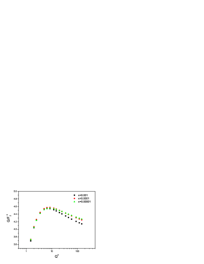
Figure 2: Plot of the ratio $G/F_{2}^{s}$ as a function of $Q^{2}$.

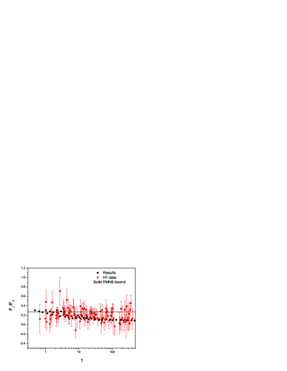
Figure 3: Ratio $F_{L}/F_{2}$ plotted as function of scaling variable $\tau$ compared with H1 data [1]. Straight line corresponds to the color dipole model bound [10].

In this paper, we obtain the ratio $G(x,Q^{2})/F_{2}^{s}(x,Q^{2})$ and $F_{L}(x,Q^{2})/F_{2}(x,Q^{2})$ and the proton structure function at NNLO analysis respectively. The analysis is performed in the range $10^{-5}\leq x\leq 10^{-2}$ and $1.5\leq Q^{2}\leq 150~{}GeV^{2}$. We should first extract the ratio $G/F_{2}^{s}$ in Fig.1 with $\tau$ variable where $\tau=\frac{Q^{2}}{Q_{0}^{2}}(\frac{x}{x_{0}})^{-\lambda}$. Here $Q_{0}^{2}=1~{}GeV^{2}$, $x_{0}=3.0\times 10^{-4}$ and $\lambda=\lambda_{s}$. The effective exponents for gluon and singlet distributions are defined with an exponent of $\lambda_{g}=0.424$ and $\lambda_{s}=0.327$ respectively [18]. These values are compatible with other results [19]. Also this ratio is plotted in Fig.2 with $Q^{2}$ at a certain representation value of fixed $x$.
In what follows the ratio $F_{L}(x,Q^{2})/F_{2}(x,Q^{2})$, with respect to Eqs.(16) and (19), is calculated and presented in Fig.3. In this figure the ratio of the structure functions compared with the H1 data [1] and with the result obtained by the color dipole model bound [10]. The error bars of the ratio $\frac{F_{L}}{F_{2}}$ are determined by the following form [11]

$$\Delta(\frac{F_{L}}{F_{2}})=\frac{F_{L}}{F_{2}}\sqrt{(\frac{\Delta F_{L}}{F_{L}})^{2}+(\frac{\Delta F_{2}}{F_{2}})^{2}},$$ (27)

where $\Delta F_{L}$ and $\Delta F_{2}$ are collected from the H1 experimental data in Ref.[1]. The good agreement between this method and the experimental data indicates that our results has a bound asymptotic behavior and it is compatible with the color dipole model bound.
In Ref.[3] the measured structure functions $F_{L}(x,Q^{2})$ for $Q^{2}\leq 35~{}GeV^{2}$ with total uncertainties below $0.3$ and $Q^{2}=45~{}GeV^{2}$ below $0.4$ are presented. The ratio $R(=\frac{F_{L}}{F_{2}-F_{L}})$ is found at $R=0.260{\pm}0.050$ which this value is constant at the region $7.10^{-5}<x<2.10^{-3}$ and $3.5\leq Q^{2}\leq 45GeV^{2}$. We know that the color dipole model has been described for virtual photon-proton scattering at low $x$ and low $Q^{2}$ values. In color dipole model the ratio $R$ lead to the bound $R\leq 0.372$ [7]. This value decrease when another approaches were developed to describe the dipole-proton cross section, such as IIM and B-SAT. Where the first one is a model based on the colour glass condensate approach to the high parton density regime and the another one is a model with the generalised impact parameter dipole saturation respectively [9]. In Ref.[24] ZEUS Collaboration is shown that the overall value of $R$ from both the unconstrained and constrained fits is $R=0.105^{+0.055}_{-0.037}$ in wide range of $Q^{2}$ values ($5\leq Q^{2}\leq 110~{}GeV^{2}$). In both the DGLAP and the dipole models the structure function $F_{L}$ and the ratio of the structure functions can be calculated. It is thus of interest to compare predictions of the different models with the data. For high $Q^{2}>10~{}GeV^{2}$, theses models agree with the data but for lower $Q^{2}$ values, there is a significant difference between the predictions.
Indeed authors of Ref.[11] have shown that for realistic dipole-proton cross-section the bound is reduced from $0.27$ to $0.22$. With respect to this method we can see from Fig.3 which the ratio structure functions lie below the EMNS bound at moderate and high values of $\tau$, and it is comparable with the EMNS bound at low values of $\tau$. In this region the data indicate a decrease of the ratio $\frac{F_{L}}{F_{2}}$ for small values of $Q^{2}$, as we do not expect for evolution equation predicted with respect to the singlet and gluon distribution behavior. This behavior allows us to speculate that there may be a need for QCD resummations beyond the conventional DGLAP equations or the need for non-linear evolution equations which take account of gluon recombination and the possibility of gluon saturation. Such effects can be described by non-linear evolution equations including higher-twist corrections at low -$x$ values [25-26]. The expectation is that such terms are important for the longitudinal structure function but not for the structure function $F_{2}$.
Indeed the introduction of higher-twist terms is one possible way to extend the DGLAP framework to low $Q^{2}$ values. Such terms have been introduced at low-$x$ values since, for the kinematics of HERA, low $Q^{2}$ is only accessed at low $x$. To better illustrate our calculations at low $Q^{2}$, we added a higher twist term in the description of the structure functions, for HERA data on deep inelastic scattering, at low $x$ and low $Q^{2}$ values. It can be clearly seen that our predictions with respect to the higher twist (HT) analyses are comparable with data at this region. The leading twist perturbative QCD predictions of the structure functions $F_{2}$ and $F_{L}$ augment by a simple higher twist term such that

$$F_{2}^{HT}=F_{2}^{DGLAP}(1+\frac{A_{2}}{Q^{2}}),$$

$$F_{L}^{HT}=F_{L}^{DGLAP}(1+\frac{A_{L}}{Q^{2}}),$$ (28)

where $A^{HT}_{2}=0.12~{}\pm~{}0.07~{}GeV^{2}$ and $A^{HT}_{L}=5.5~{}\pm~{}0.6~{}GeV^{2}$ are free parameters at NNLO [25-26]. Using the HT terms in Eqs.16 and 19, we can evaluate the HT corrections to the ratio $G/F_{2}^{s}$ and $F_{L}/F_{2}$ as we have

$$\mathrm{Eq.(16)} \Rightarrow \lambda_{gs}D_{qg}(x,Q^{2})K^{2}(x,Q^{2})\frac{1}{1+A^{HT}_{2}/Q^{2}}$$ (29)

$$+[\lambda_{gs}C_{qq}(x,Q^{2})-A_{gg}(x,Q^{2})]K(x,Q^{2})$$

$$-(1+A^{HT}_{2}/Q^{2})B_{gq}(x,Q^{2})=0,$$

and

$$\mathrm{Eq.(19)} \Rightarrow \frac{F_{L}(x,Q^{2})}{F_{2}(x,Q^{2})}=\frac{1}{1+A^{HT}_{L}/Q^{2}}\{(1+A^{HT}_{2}/Q^{2})$$ (30)

$$[C_{L,q}(x,\alpha_{s}(Q^{2})){\otimes}x^{\lambda_{s}}]+<e^{2}>K(x,Q^{2})$$

$$[C_{L,g}(x,\alpha_{s}(Q^{2})){\otimes}x^{\lambda_{g}}]\}.$$

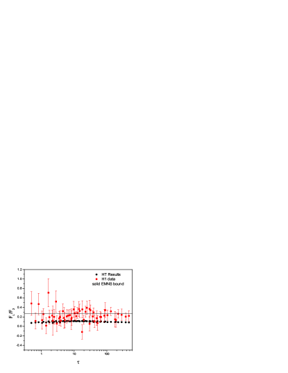
Figure 4: The HT data of the ratio plotted as function of scaling variable $\tau$ compared with H1 data [1]. Straight line corresponds to the color dipole model bound [10].

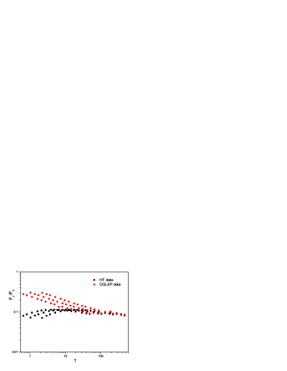
Figure 5: The DGLAP and HT data for the ratio plotted as function of $\tau$.

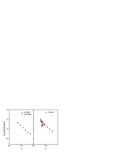
Figure 6: The proton structure function $F_{2}(x,Q^{2})$ for $Q^{2}=20~{}GeV^{2}$ compared with H1 data [1, 4] where accompanied with total errors.

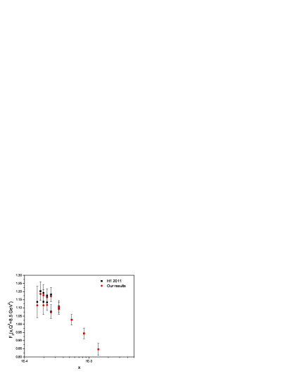
Figure 7: The proton structure function $F_{2}(x,Q^{2})$ for $Q^{2}=8.5~{}GeV^{2}$ compared with H1 data [3] where accompanied with total errors.

The results are shown in Fig.4. In this figure the HT predictions of the ratio $\frac{F_{L}}{F_{2}}$ presented on the H1 measurement, where a decrease of the ratio for small $Q^{2}$ values is observable. Comparison of the DGLAP data with HT data are shown in Fig.5.
Having checked that the ratio method obtained reproduced satisfactorily the existing DIS reduced cross section on the electron-proton collisions in upper $x$ domain at fixed $Q^{2}$ values. We shall now use it to make predictions for these values as expected there are no data for electron- proton collisions in this region. The results are depicted in Table I. In this table we compared results with Ref.4 data and obtained the starting $x-Q^{2}$ points as this method can be prediction data at extrapolation points . These results are comparable with literature as accompanied with total errors. In figure 6, the proton structure function have been shown and compared at $Q^{2}=20~{}GeV^{2}$ with H1 2001 and H1 2014 data [1,4] respectively. These figures indicates that the obtained results from present analysis based on DGLAP bound are in good agreements with the ones obtained by HERA data. A comparison has also been shown at $Q^{2}=8.5~{}GeV^{2}$ in figure 7 and compared with H1 2011 data [3] as accompanied with total errors. We see that all predictions are consistent with the large $y$ data.

.6 4. Heavy flavor contribution

As our further research activities we hope to study the ratio of structure functions to get an analytical solutions for heavy quark contributions of the structure functions. When the virtual photon interacts indirectly with a gluon in the proton then a heavy quark pair produced via the direct boson-gluon fusion processes. At low-$x$ this behavior is related to the growth of gluon distribution via the $g\rightarrow q_{H}\overline{q}_{H}~{}(H=c,b)$ transition [27-28]. Then the perturbative predictions for $F_{L}(x,Q^{2})$ at the $N_{f}=3$ light quark flavor sector and heavy contribution can be written as

$$x^{-1}F_{L}=C_{L,ns}{\otimes}q_{ns}+\frac{2}{9}(C_{L,q}{\otimes}q_{s}+C_{L,g}{\otimes}g)+x^{-1}F_{L}^{H}.$$

Also the heavy quark contribution to the total structure functions is $F_{2}(x,Q^{2})=F_{2}^{\mathrm{light}}+F_{2}^{\mathrm{Heavy}}$ where ‘light’ refers to the common $u;d;s$ (anti)quarks and gluon initiated contributions at fixed flavor number scheme. The heavy quark contributions at small-$x$ are given by

$$F_{k}^{H}(x,Q^{2}) = \frac{Q^{2}\alpha_{s}(\mu^{2})}{4\pi^{2}m^{2}_{H}}\int_{ax}^{1}\frac{dy}{y}yg(y,\mu^{2})e^{2}_{H}\{C_{k,g}^{(0)}$$ (32)

$$+4\pi\alpha_{s}(\mu^{2})[C_{k,g}^{(1)}+\overline{C}_{k,g}^{(1)}\ln\frac{\mu^{2}}{m^{2}_{H}}]+...\}$$

$$,~{}(k=2,L).$$

Here $e_{H}$ denotes the heavy charge and $m_{H}$ denotes the heavy quark mass [2]. The lower limit of integration is given by $y_{min}=ax=(1+4\frac{m_{H}^{2}}{Q^{2}})x$ and the mass factorization scale $\mu$ which has been put equal to the renormalization scale is assumed to be either $\mu^{2}=4m^{2}_{H}$ or $\mu^{2}=4m^{2}_{H}+Q^{2}$.
Now discuss the bound for the ratio $F_{L}/F_{2}$ for $n_{f}=3+\mathrm{Heavy}$, as

$$\frac{F_{L}^{\mathrm{light}+c}}{F_{2}^{\mathrm{light}+c}} = \frac{F_{L}^{N_{f}=3}+F_{L}^{c}}{F_{2}^{N_{f}=3}+F_{2}^{c}}$$ (33)

$$=\frac{F_{L}^{N_{f}=3}/F_{2}^{N_{f}=3}+F_{L}^{c}/F_{2}^{N_{f}=3}}{1+F_{2}^{c}/F_{2}^{N_{f}=3}},$$

when $m_{c}^{2}<\mu^{2}<m_{b}^{2}$ and

$$\frac{F_{L}^{\mathrm{light}+c+b}}{F_{2}^{\mathrm{light}+c+b}} = \frac{F_{L}^{N_{f}=3}+F_{L}^{c}+F_{L}^{b}}{F_{2}^{N_{f}=3}+F_{2}^{c}+F_{2}^{b}}$$

$$=\frac{F_{L}^{N_{f}=3}/F_{2}^{N_{f}=3}+F_{L}^{c}/F_{2}^{N_{f}=3}+F_{L}^{b}/F_{2}^{N_{f}=3}}{1+F_{2}^{c}/F_{2}^{N_{f}=3}+F_{2}^{b}/F_{2}^{N_{f}=3}},$$

when $m_{b}^{2}<\mu^{2}<m_{t}^{2}$. The ratio $\frac{F_{L}^{N_{f}}}{F_{2}^{N_{f}}}$ not only mentioned earlier in Eq.(19) for $N_{f}=4$ but also it will be consider here for $N_{f}=3$.
The ratio of the heavy flavor structure functions are described by a convolution between the gluon distribution and the heavy Wilson coefficients as we have

$$\frac{F_{k}^{H}}{F_{2}^{N_{f}=3}} = \frac{G(x,\mu^{2})}{F_{2}^{N_{f}=3}}\{C_{k,g}^{H}(x,\frac{Q^{2}}{\mu^{2}})\otimes x^{\lambda_{g}}\}$$

$$=K(x,Q^{2})[\mathrm{Eq.16~{}for~{}N_{f}=3}]\{C_{k,g}^{H}(x,\frac{Q^{2}}{\mu^{2}})\otimes x^{\lambda_{g}}\}.$$

In Table II the effects of heavy quarks on the ratio of structure functions are considered. We observe that the bottom quark effect on the ratio is negligible in the wide range of $Q^{2}$ values. In the present analysis we use $m_{c}=1.3~{}GeV$ and $m_{b}=4.5~{}GeV$, therefore

$$\frac{F_{L}^{\mathrm{light}+c+b}}{F_{2}^{\mathrm{light}+c+b}}{\simeq}\frac{F_{L}^{\mathrm{light}+c}}{F_{2}^{\mathrm{light}+c}}.$$ (36)

In Table III we observe that the bound is changed when the inclusion charm mass effects is going in the bound. The charm effects in the bound of ratio show that in the wide range of $Q^{2}$ values we have this behavior as

$$\frac{F_{L}}{F_{2}}|_{{N_{f}=3+c}}~{}{\leq}~{}\frac{F_{L}}{F_{2}}|_{{N_{f}=4}}.$$ (37)

We note that the ratio $F_{L}/F_{2}$ in $N_{f}=3+c$ is approximately equivalent to the ratio in $N_{f}=4$ at high-$Q^{2}$ values. A comparison of the various contributions to the ratio shows that for low-$Q^{2}$ values the charm quark contribution in the ratio is about $12\%$ or less. Therefore the charm effect in the bound decrease as $Q^{2}$ increases. Indeed the ratio bound is lower than EMNS bound when the charm mass effects are taken into account.

.7 5. Conclusion

In this paper we have found that there is in general an analytical relation between the gluon distribution function and singlet structure function at low $x$ region into the effective exponents. The ratio of the structure functions into the DGLAP evolution equations at small $x$ at NNLO analysis is studied and compared with EMNS bound in this region. Results are comparable with the experimental data and they are lower than EMNS bound at high-$Q^{2}$ values. Our results are very close to the bounds for low-$Q^{2}$ values as we have discussed the meaning of these findings from the points of view of higher twist terms added to the structure functions. Having checked that this model gives a good description of the ratio $F_{L}/F_{2}$ then we predict $F_{2}(x,Q^{2})$ with respect to the reduced cross section measured in HERA collisions. We observed that the general solutions are comparable with the available experimental data. Finally we discussed the charm quark effects in bounds at high and low-$Q^{2}$ values.

.8 Appendix A

The explicit forms of the functions $A_{gg}(x,Q^{2})$, $B_{gq}(x,Q^{2})$, $C_{qq}(x,Q^{2})$ and $D_{qg}(x,Q^{2})$ are defined by

$$A_{gg}(x,Q^{2}) = P_{gg}(x,\alpha_{s}(Q^{2})){\otimes}x^{\lambda_{g}}$$

$${\equiv}{\int_{x}^{1}}dzP_{gg}(z,\alpha_{s}(Q^{2})){z}^{\lambda_{g}},$$

$$B_{gq}(x,Q^{2}) = P_{gq}(x,\alpha_{s}(Q^{2})){\otimes}x^{\lambda_{s}}$$

$${\equiv}{\int_{x}^{1}}dzP_{gq}(z,\alpha_{s}(Q^{2})){z}^{\lambda_{s}},$$

$$C_{qq}(x,Q^{2}) = P_{qq}(x,\alpha_{s}(Q^{2})){\otimes}x^{\lambda_{s}}$$

$${\equiv}{\int_{x}^{1}}dzP_{qq}(z,\alpha_{s}(Q^{2})){z}^{\lambda_{s}},$$

$$D_{qg}(x,Q^{2}) = P_{qg}(x,\alpha_{s}(Q^{2})){\otimes}x^{\lambda_{g}}$$ (38)

$${\equiv}{\int_{x}^{1}}dz2N_{f}P_{qg}(z,\alpha_{s}(Q^{2})){z}^{\lambda_{g}}.$$

where the strong coupling constant $\alpha_{s}$ and splitting functions up to NNLO are given in Ref.[14].

.9 References

1. V. Andreev et al. [H1 Collab.], Eur. Phys. J. C74(2014)2814.
2. H. Abramowicz et al. [H1 and ZEUS Collab.], Eur. Phys. J. C 75(2015)580.
3. F.D. Aaron et al. [H1 Collaboration], phys.Lett.B665, 139(2008); Eur.Phys.J.C71,1579(2011).
4. C.Adloff et al. [H1 Collaboration], Eur.Phys.J.C21, 33(2001).
5. V.Tvaskis et al., Phys.Rev.C97, 045204(2018).
6. N.N.Nikolaev and B.G.Zakharov, Z.Phys.C49, 607(1991); Z.Phys.C53, 331(1992).
7. C.Ewerz and O.Nachtmann, Phys.Lett.B648, 279(2007).
8. C.Ewerz, A. von Manteuffel and O.Nachtmann, Phys.Rev.D77, 074022(2008).
9. K.Golec-Biernat and W$\mathrm{\ddot{u}}$sthoff, Phys.Rev.D59, 014017(1999); E. Iancu, K. Itakura, and S. Munier, Phys. Lett. B590, 199(2004); H. Kowalski, L.Motyka, and G.Watt, Phys. Rev. D74, 074016(2006).
10. C.Ewerz et al., Phys.lett.B720, 181(2013).
11. M.Niedziela and M.Praszalowicz, Acta Phys.Polon. B46, 2019(2015).
12. Yu.L.Dokshitzer, Sov.Phys.JETP 46, 641(1977); G.Altarelli and G.Parisi, Nucl.Phys.B 126, 298(1977); V.N.Gribov and L.N.Lipatov, Sov.J.Nucl.Phys. 15, 438(1972).
13. G.Altarelli and G.Martinelli, Phys.Lett. B76, 89(1978).
14. G. R. Boroun and B. Rezaei, Eur. Phys. J. C73, 2412(2013); G. R. Boroun and B. Rezaei, Eur. Phys. J. C72(2012)2221.
15. S.Shoeibi, et al., Phys.Rev.D7, 074013 (2018); H.Khanpour et al., Eur.Phys. J.C78, 7(2018); S.M. Mossavi Nejad et al., Phys.Rev.C94, 045201(2016); F.Taghavi-Shahri et al., Phys.Rev.D93, 114024 (2016); H.Khanpour et al., Phys.Rev.C95, 035201(2017); J.Sheibaniet al., Phys.Rev.C98, 045211(2018).
16. G.R.Boroun Phys.Rev.C97, 015206 (2018); B.Rezaei and G.R.Boroun, arXiv:1811.02785(2018).
17. A. Vogt et al., Nucl. Phys. B691(2004)129.
18. P.D.B.Collins, Cambridge University Press, Cambridge (1977).
19. N. N. Nikolaev and W. Sch fer, Phys. Rev. D 74, 014023 (2006); E.Gotsman et al., arXiv:1712.06992(2017); H.Kowalski et al., arXiv:1707.014460(2017).
20. G. R. Boroun, Eur. Phys. J. A50, 69(2014).
21. M. Devee and J. K. Sarma, Eur. Phys. J. C72, 2036(2012).
22. L. Machahari and D.K.Choudhury, Eur.Phys.J.A54, 69(2018).
23. S. Moch et al., Phys. Lett. B606, 123(2005).
24. H.Abromowicz et al. [ZEUS Collaboration], Phys.Rev.D9, 072002(2014).
25. A.M.Cooper-Sarkar, arXiv:1605.08577v1 [hep-ph] 27 May 2016; I.Abt et.al., arXiv:1604.02299v2 [hep-ph] 11 Oct 2016.
26.F.D. Aaron et al. [H1 Collaboration], Eur.Phys.J. C63, 625(2009).
27. N.N.Nikolaev and V.R.Zoller, Phys.Atom.Nucl73, 672(2010); A. Y. Illarionov and A. V. Kotikov, Phys.Atom.Nucl. 75, 1234 (2012); N.Ya.Ivanov, and B.A.Kniehl, Eur.Phys.J.C59, 647(2009); L.P.Kaptari et al., arXiv:1812.00361[hep-ph](2018).
28. G.R.Boroun, B.Rezaei, JETP,Vol.115, No.7, PP.427 (2012); Nucl.Phys.B857, 143(2012); Eur.Phys.J.C72, 2221 (2012); EPL100,41001(2012); Nucl.Phys.A929, 119(2014); G.R.Boroun, Nucl.Phys.B884, 684(2014).

Table 1: The proton structure function determined based on the reduced cross section data that accompanied with total errors.

$Q^{2}(GeV^{2})$	$x$	$y$	$\widetilde{\sigma}$	$\Delta(\%)$	$F_{2}$(Ref.4)	$F_{2}$
2	0.0000327	0.675	0.805	7.4	—-	0.911
2	0.0000500	0.442	0.823	3.5	0.851	0.859
2.5	0.0000409	0.675	0.899	7.4	—-	1.009
2.5	0.0000500	0.552	0.859	3.7	0.909	0.921
3.5	0.0000573	0.675	0.897	7.0	—-	0.955
3.5	0.0000800	0.483	0.925	2.9	0.964	0.971
5	0.0000818	0.675	1.019	6.6	—-	1.118
5	0.000130	0.425	1.015	2.4	1.043	1.045
8.5	0.000139	0.675	1.097	4.9	—-	1.186
8.5	0.000200	0.470	1.152	2.9	1.193	1.189
12	0.000161	0.825	1.226	5.8	—-	1.377
12	0.000197	0.675	1.269	3.5	—-	1.362
12	0.000320	0.415	1.217	2.0	1.249	1.243
15	0.000201	0.825	1.255	5.2	—-	1.399
15	0.000246	0.675	1.361	3.3	—-	1.454
15	0.000320	0.519	1.283	2.4	1.342	1.328
20	0.000268	0.825	1.313	5.2	—-	1.451
20	0.000328	0.675	1.383	2.7	—-	1.470
20	0.000500	0.443	1.285	2.0	1.324	1.313
25	0.000335	0.825	1.379	5.9	—-	1.515
25	0.000410	0.675	1.371	2.6	—-	1.452
25	0.000500	0.553	1.345	2.4	1.417	1.393
35	0.000574	0.675	1.473	2.7	—-	1.553
35	0.000800	0.484	1.354	2.2	1.405	1.386

Figure 1: Plot of the ratio $G/F_{2}^{s}$ vis $\tau$.

Table 2: The ratio $F_{k}^{H}/F_{2}$ determined in the case $N_{f}=3$ for different values of $Q^{2}$.

$Q^{2}(GeV^{2})$	$F_{2}^{b}/F_{2}$	$F_{L}^{b}/F_{2}$	$F_{2}^{c}/F_{2}$	$F_{L}^{c}/F_{2}$
2	0.00008	0.0000005	0.013	0.0008
20	0.0016	0.00009	0.079	0.015
200	0.012	0.002	0.130	0.025
400	0.015	0.003	0.138	0.025

Table 3: The ratio $F_{L}/F_{2}$ determined in the case $N_{f}=3$ and $N_{f}=3+\mathrm{charm}$ and compared with the case $N_{f}=4$ for different values of $Q^{2}$.

$Q^{2}(GeV^{2})$	$F_{L}/F_{2}|_{N_{f}=3}$	$F_{L}/F_{2}|_{N_{f}=3+c}$	$F_{L}/F_{2}|_{N_{f}=4}$
1.5	0.275	0.273	0.305
2	0.247	0.245	0.281
4	0.192	0.189	0.229
10	0.142	0.143	0.174
20	0.116	0.122	0.144
50	0.093	0.104	0.116
90	0.083	0.096	0.103
120	0.078	0.092	0.097
150	0.075	0.090	0.093
200	0.071	0.086	0.088