Neutron gas and pairing

Abstract

We study the emergence of neutron gas effects in the description of nuclei with large neutron excess within the Bardeen-Cooper-Schrieffer approach. We consider Ni and Sn isotopes where, in the literature, these effects have been found. We investigate the role of the single particle states with positive energy generating the neutron gas, and we find that the contribution of these states is numerically irrelevant for the various observables that we evaluate.

I Introduction

The study of exotic nuclei close to the neutron-drip line has generated great interest in these last years. For these systems, uncommon nuclear properties have been predicted and some of them have been experimentally identified Gade and et al. (2008); Sorlin and Porquet (2008); Wienholtz and et al. (2013); Steppenbeck and et al. (2013).

The theoretical description of these nuclei with a large neutron excess requires an accurate treatment of pairing correlations. Among the various approaches built to handle these correlations, one of the most used is that based on the Bardeen-Cooper-Schrieffer (BCS) theory Bohr et al. (1958); Rowe (1970); Ring and Schuck (1980); Suhonen (2007). In this approach, the nucleon-nucleon pairing interaction modifies the occupation probabilities of a set of single particle (s.p.) states generated within a mean-field (MF) model.

Despite the fact that the MF+BCS approach is widely utilized to study nuclei throughout the whole nuclear chart, some questions have been raised on its reliability in the description of neutron rich nuclei. These doubts, in the literature, have been summarized under the name of neutron, or particle, gas problem Dobaczewski et al. (1984); Dobaczewski et al. (1996a, b); Dobaczewski (1999).

To clarify the origin and the details of this problem, let us consider the one-body density matrix (OBDM) defined as Arias de Saavedra et al. (2007)

$$\rho({\bf r},{\bf r}^{\prime})\,=\,\frac{A}{\langle\Psi|\Psi\rangle}\int{\rm d}^{3}r_{2}\,\cdots{\rm d}^{3}r_{A}\,\Psi^{*}({\bf r},{\bf r}_{2},\cdots,{\bf r}_{A})\,\Psi({\bf r}^{\prime},{\bf r}_{2},\cdots,{\bf r}_{A})\,,$$ (1)

where we have indicated with $\Psi$ the eigenstates of the hamiltonian describing a finite system of $A$ interacting nucleons. In the ground state of a bound nucleus, the nucleons are localized in space, and, therefore, the OBDM verifies the conditions

$$\lim_{{\bf r}\rightarrow\infty}\rho({\bf r},{\bf r}^{\prime})\,=\,\lim_{{\bf r}^{\prime}\rightarrow\infty}\rho({\bf r},{\bf r}^{\prime})\,=\,0\,.$$ (2)

In the MF approach the many-body hamiltonian is simplified: it can be written as a sum of non-interacting s.p. hamiltonians and the many-body wave functions can be expressed as Slater determinants of eigenstates $\phi_{\alpha}({\bf r})$ of these s.p. hamiltonians. In this case, the OBDM assumes the form:

$$\rho^{\rm MF}({\bf r},{\bf r}^{\prime})\,=\,\sum_{\alpha}\,{(v_{\alpha}^{\rm MF})^{2}}\,\phi^{*}_{\alpha}({\bf r})\,\phi_{\alpha}({\bf r}^{\prime})\,\Theta(\epsilon_{\rm F}-\epsilon_{\alpha})\,,$$ (3)

where we have indicated with $\epsilon_{\rm F}$ the Fermi energy, with ${(v_{\alpha}^{\rm MF})^{2}}$ and $\epsilon_{\alpha}$, respectively, the occupation probability and the energy of the s.p. state $\phi_{\alpha}({\bf r})$, and with $\Theta(\alpha)$ the step function. In a MF model all the states up to the Fermi surface are fully occupied, ${(v_{\alpha}^{\rm MF})^{2}}=1$ if $\epsilon_{\alpha}\leq\epsilon_{\rm F}$, and those above it are completely empty, ${(v_{\alpha}^{\rm MF})^{2}}=0$ if $\epsilon_{\alpha}>\epsilon_{\rm F}$.

If the set of s.p. states is obtained in Hartree-Fock (HF) calculations, a variational procedure that consists in finding the energy minimum by modifying the s.p. wave functions is performed. The values of the occupation probabilities remain unaltered. Since the $\phi_{\alpha}$ states below the Fermi surface, i.e. those involved in the sum in Eq. (3), are bound, they are localized in space and, consequently, the boundary conditions of Eq. (2) are still satisfied.

In the BCS approach, the pairing acts on the MF picture by changing the values of the occupation probabilities, while the s.p. wave functions are not modified. The OBDM is given by the expression

$$\rho^{\rm BCS}({\bf r},{\bf r}^{\prime})\,=\,\sum_{\alpha}\,{(v_{\alpha}^{\rm BCS})^{2}}\,\phi^{*}_{\alpha}({\bf r})\,\phi_{\alpha}({\bf r}^{\prime})\,.$$ (4)

It is worth noting that, at variance with the MF expression (3), in Eq. (4) the sum does not have an upper limit. This means that, in principle, all the s.p. wave functions contribute to $\rho^{\rm BCS}$, even those in the continuum which have an oscillating behavior at the boundaries. Under these circumstances, compliance with the conditions (2) cannot be guaranteed for $\rho^{\rm BCS}$ and this is the source of the neutron gas problem.

This problem is absent in Hartree-Fock-Bogoliubov (HFB) theory, the other widely used approach which treats pairing correlations Ring and Schuck (1980). In this case, the variational principle is applied by changing both s.p. wave functions and occupation probabilities at once. The OBDM obtained in the HFB theory can be written as

$$\rho^{\rm HFB}({\bf r},{\bf r}^{\prime})\,=\,\sum_{\alpha}\,{(v_{\alpha}^{\rm HFB})^{2}}\,\zeta^{*}_{\alpha}({\bf r})\,\zeta_{\alpha}({\bf r}^{\prime})\,,$$ (5)

formally equivalent to the BCS density given in Eq. (4). However, in this case, the wave functions $\zeta_{\alpha}({\bf r})$ belong to the so-called “canonical basis” which, by construction, are limited in space. For this reason in HFB calculations the boundary properties of Eq. (2) are always fulfilled.

Summarizing, we can say that the BCS theory considers the presence of free nucleons even in the nuclear ground state. In Refs. Dobaczewski et al. (1984); Dobaczewski et al. (1996a, b); Dobaczewski (1999) it has been pointed out that this feature, in neutron rich nuclei, affects the values of the neutron distribution radii, which appear to be too large with respect to those found in HFB calculations, and also the asymptotic behavior of the OBDMs showing long distance tails abnormally high. These facts have been considered as evidences of the neutron gas problem.

Even though these considerations would induce us to abandon the MF+BCS approach in favour of the HFB one, there are some nice features of the former approach that make it still widely utilized. It is easier to solve the BCS equations than those of the HFB theory, the physical interpretation of the results is more direct and the many-body wave functions are more handily usable to calculate nuclear excited states as, for example, within the Quasi-Particle Random Phase Approximation (QRPA) theory.

Furthermore, in our experience, we used the MF+BCS approach to study various nuclei in different regions of the nuclear chart Anguiano et al. (2014, 2015, 2016); De Donno et al. (2017) and we never encountered problems related to the presence of neutron gas. This result was quite astonishing, and induced us to study the quantitative relevance of this problem in order to test the reliability of the MF+BCS approach and define the limits of validity in its application.

We have carried out our investigation by comparing results obtained with both MF+BCS and HFB approaches by using various types of nucleon-nucleon and pairing interactions. We present here the results that we have obtained for those isotopes considered in Refs. Dobaczewski et al. (1984); Dobaczewski et al. (1996a, b); Dobaczewski (1999) where the neutron gas problem was identified.

Since the quantitative relevance of the neutron gas effects is the subject of our investigation, we discuss with some detail in Sec. II those aspects of our calculations related to their numerical stability. In Sec. III, we compare our results to those found in the literature Dobaczewski et al. (1984); Dobaczewski et al. (1996a, b); Dobaczewski (1999). First we consider neutron radii and density distributions in Ni and Sn isotopes. To verify the quantitative effects of the neutron gas in other observables, we present the proton elastic scattering cross sections calculated for the ¹⁵⁰Sn nucleus. We summarize our results in Sec. IV and we conclude that, from the quantitative point of view, the neutron gas problem is irrelevant and MF+BCS calculations are reliable in all the regions of the nuclear chart table.

II Details of the calculations

The aim of our study is the evaluation of the quantitative relevance of the effects induced by the neutron gas in MF+BCS calculations. For this reason, the numerical reliability of the computational methodologies adopted to solve the various equations defined by the model is an essential ingredient of our investigation. Therefore, in this section, we present in detail all the key ingredients of our calculations and we discuss the implications of the various inputs either of physics or numerical type.

In the present work, we have considered only spherical nuclei. For each of them a MF s.p. basis has been generated by solving HF equations. By exploiting the spherical symmetry of the system, the HF equations have been expressed as integro-differential non-linear equations depending only on a single variable, the distance from the center of coordinates, $r$. We have defined a maximum value, ${R_{\rm box}}$, of this distance, and in this position we have imposed infinite well boundary conditions. The value of ${R_{\rm box}}$ is one of the numerical inputs of our approach and depends on the size of the nucleus investigated.

The HF equations are solved iteratively, by considering only the s.p. wave functions with s.p. energies $\epsilon_{\alpha}\leq\epsilon_{\rm F}$. The numerical solution of these equations is obtained by using the plane wave expansion technique developed in Refs. Guardiola and Ros (1982); Guardiola et al. (1982). The number of plane waves considered in the expansion is equal to the number of mesh points employed to describe the $r$ space up to ${R_{\rm box}}$. This is the second, numerical, input of our approach and we have found that a mesh size of the order of $0.1\,$fm is enough to ensure the numerical stability of the HF results for the nuclei studied. This technique allows a treatment of the non-local Fock-Dirac term of the HF equations without any approximation.

In our procedure, when the minimum of the binding energy is found, and for this purpose we have chosen a convergence value of $1\,$eV, the Hartree and the Fock-Dirac potential terms Ring and Schuck (1980), built with the s.p. wave functions with $\epsilon_{\alpha}\leq\epsilon_{\rm F}$, are used to calculate also the s.p. wave functions and energies of the states above the Fermi surface. Because of the infinite well boundary conditions, the s.p. spectra are discrete, even for energies larger than zero. While the bound s.p. states are extremely stable against the choice of the ${R_{\rm box}}$ value (we observe a change in the value of the s.p. energy of about one part on a million for a 20% change of ${R_{\rm box}}$), the s.p. states with positive energies are very sensitive to it. It is worth pointing out that this affects all the theories making use of the full set of HF, or more in general MF, s.p. states because all of them have to deal with the “discretized continuum” part of the s.p. spectrum.

In our approach, the BCS equations are solved by means of an iterative procedure and by using standard numerical methods Suhonen (2007). The configuration space we have considered is composed by the set of discrete s.p. wave functions, with both negative and positive energies, generated by the previously described HF calculations. The value of the box size required for the integrations in $r$-space is the same as that employed in the HF calculations. The only new input is the maximum value of the energy of the s.p. states considered, ${\epsilon_{\rm max}}$, which determines the size of the configuration space.

In the present study, the effective nucleon-nucleon interaction that we have considered is a finite-range force of Gogny type, specifically in its D1S parameterization. This is the most traditional, and widely used, Gogny force, and its parameters have been chosen to fit experimental values of binding energies and charge root mean square (rms) radii belonging to a large body of nuclei in all the regions of the nuclear chart Berger et al. (1991). We have consistently used this interaction in both steps of our calculations, HF and BCS. As is it clearly discussed in Ref. Dechargé and Gogny (1980), the finite-range feature of this interaction induces a natural cut in the coupling to high energy s.p. states due to pairing. This avoids to insert in the theory additional physics inputs, such as a specific pairing interaction related to the size of the s.p. configuration space Dobaczewski et al. (1984); Dobaczewski et al. (1996a, b).

				$\epsilon_{\rm max}$ (MeV)
nucleus		$R_{\rm box}$ (fm)		8	10	12
22O		10		3.006	3.007	3.007
		12		3.008	3.008	3.008
		14		3.010	3.008	3.008
86Ni		20		4.535	4.535	4.535
		22		4.544	4.544	4.543
		24		4.550	4.550	4.550
150Sn		23		5.289	5.290	5.291
		25		5.294	5.296	5.298
		27		5.301	5.304	5.306

Table 1: Neutron rms radii, expressed in fm, for the ²²O, ⁸⁶Ni and ¹⁵⁰Sn isotopes, obtained in HF(D1S)+BCS(D1S) calculations for different values of the parameters $R_{\rm box}$ and $\epsilon_{\rm max}$. The underlined values are those obtained by considering the values of $R_{\rm box}$ and $\epsilon_{\rm max}$ used in our standard calculations.

We have studied the numerical stability of the neutron rms radii values obtained in our HF+BCS calculations against the changes in the values of the parameters $R_{\rm box}$ and $\epsilon_{\rm max}$. We show in Table 1 the values of these radii for the nuclei ²²O, ⁸⁶Ni and ¹⁵⁰Sn which have a large neutron excess and have been selected to be representative of three different regions of the nuclear chart. In the table, we have underlined the values obtained in our standard calculations, i. e. those where we have verified the convergence of all the quantities obtained in BCS, such as pairing gaps, quasi-particle energies, occupation probabilities, etc. The other values shown in the table have been obtained by varying ${R_{\rm box}}$ and ${\epsilon_{\rm max}}$. The largest relative differences with respect to the standard values are below 0.2%. We have also checked that the neutron densities obtained for a given $R_{\rm box}$ and the three values of $\epsilon_{\rm max}$ shown in the table do not change significantly. Henceforth, we have indicated as HF(D1S)+BCS(D1S) the calculations carried out with $\epsilon_{\rm max}=10\,$MeV, and with a value of $R_{\rm box}$, obviously different for each nucleus investigated, but properly selected to guarantee the convergence of the results.

In the next sections we shall compare our HF(D1S)+BCS(D1S) results with those of a standard HFB calculation using the D1S interaction and collected in the public compilation of Ref. Hilaire and Girod . We have labelled these as reference results and indicated them as HFB^ref(D1S).

For a further comparison, we have carried out HFB calculations with the D1S interaction by using the code HFBAXIAL Robledo (2002). We have labelled HFB(D1S) the corresponding results. In this approach, the HFB equations are solved by making an expansion on a harmonic oscillator basis. In this case, we have investigated the convergence of the results with respect to the number of expansion terms, $N_{\rm ho}$, which plays a role analogous to that of $R_{\rm box}$ in our HF(D1S)+BCS(D1S) calculations.

To analyze the effects due to the range of the interaction used in the HFB approach, a further benchmark comparison has been carried out with the results obtained with the Skyrme interaction SLy5 Chabanat et al. (1998). For these calculations, which we have labelled HFB(SLy5), the code HFBRAD has been used Bennaceur and Dobaczewski (2005). As is often the case in HFB when a zero-range effective nucleon-nucleon interaction is used Dobaczewski et al. (1984); Dobaczewski et al. (1996a, b); Bennaceur and Dobaczewski (2005), the force that we have considered in the pairing sector is not SLy5. We have adopted a volume pairing field that follows the shape of the nuclear density, and we have considered the input variables selected for the test run in Ref. Bennaceur and Dobaczewski (2005). In HFBRAD the HFB equations are solved in $r$-space, we have used an integration step of $0.1\,$fm, and we have studied the convergence of the results with respect to the values of $R_{\rm box}$.

III Results

III.1 Neutron rms radii and densities of Ni isotopes

Neutron rms radii of Ni isotopes with large neutron excess have been investigated in the past in connection with the emergence of the neutron gas problem Dobaczewski et al. (1996a). In Fig. 1 we show the results obtained for the even-even Ni isotopes with $A$ varying from 50 to 90 (i. e., the neutron number $N$ varying from 22 to 62). In panel (a) we compare our HF(D1S)+BCS(D1S) results calculated by using two different values of the box size, specifically $R_{\rm box}=12\,$fm (solid green diamonds) and $20\,$fm (solid red triangles), with the reference values HFB^ref(D1S) (solid black squares). In the inset, we show the corresponding relative differences, which are well below 1%, in absolute value, except for $R_{\rm box}=20$ fm and $N>58$ where they slowly increase with $N$ up to about $4\%$ for ⁹⁰Ni. A similar difference between HF+BCS and HFB calculations using the SIII Skyrme interaction was found by Grasso et al. Grasso et al. (2001).

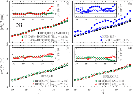
Figure 1: Neutron rms radii for the Ni isotopes. In all the panels, the reference values taken from the AMEDEE database Hilaire and Girod are indicated by the solid black squares. In panel (a), solid green diamonds and solid red triangles show the HF(D1S)+BCS(D1S) results, with $R_{\rm box}=12$ and $20\,$fm, respectively. In panel (b), open and solid blue circles indicate the results of Ref. Dobaczewski et al. (1996a) corresponding, respectively, to HFB and HF+BCS calculations carried out with the SkP Skyrme interaction. In panel (c), open green diamonds and open red triangles indicate the results of HFB calculations carried out with the code HFBRAD Bennaceur and Dobaczewski (2005) by using the SLy5 Skyrme interaction and $R_{\rm box}=12$ and $20\,$fm, respectively. In panel (d) open green diamonds and open red triangles show HFB results obtained with the D1S interaction by using the code HFBAXIAL Robledo (2002) with $N_{\rm ho}=8$ and $17$, respectively. In the insets we show the relative differences with the reference results. The values indicated by the solid blue circles in the inset of panel (b) are divided by 3 in order to fit in the scale of the figure.

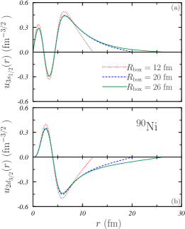
Figure 2: Wave functions of the neutron $3s_{1/2}$ (a) and $2d_{3/2}$ (b) s.p. states for the ⁹⁰Ni isotope obtained in our HF(D1S) calculations, with $R_{\rm box}=12$ (dotted red lines), 20 (dashed blue lines) and $26\,$fm (solid green lines).

The results of panel (a) should be directly compared with those of panel (b) where we show the neutron rms radii of Ref. Dobaczewski et al. (1996a), obtained by using the Skyrme SkP interaction. In this panel, the open blue circles indicate the HFB(SkP) results and the solid blue circles those of the HF(SkP)+BCS(SkP) calculations. The relative differences between the results of Ref. Dobaczewski et al. (1996a) and the reference values (indicated as in panel (a) with the solid black squares) are shown in the inset. While the HFB(SkP) results differ from the HFB^ref(D1S) by $\sim 2\%$ at most, in the case of the HF(SkP)+BCS(SkP) the relative difference is above $15\%$ for $N=62$ (or $A=90$), more than three times larger than our result for $R_{\rm box}=20\,$fm. These relative differences are also rather large, well above 10%, for the isotopes with $N=38-46$ ($A=66-74$) while our HF(D1S)+BCS(D1S) results are very close to the HFB^ref(D1S) data, independently of the value of $R_{\rm box}$.

The large disagreement between the HF(SkP)+BCS(SkP) and HFB(SkP) neutron rms radii shown in Fig. 1(b) has been considered as an evidence of the neutron gas problem Dobaczewski et al. (1996a). On the other hand, also the, much smaller, increase in the neutron rms radii, starting from the ⁸⁶Ni isotope, of our HF(D1S)+BCS(D1S) calculations for $R_{\rm box}=20\,$fm with respect to the results found for $R_{\rm box}=12\,$fm, could be interpreted as indication of such neutron gas effects. However, to a large extent, this is due to a lack of numerical convergence. In fact, a similar situation is observed in the panel (c) of Fig. 1 where the complete sequence of Ni neutron rms radii obtained within a HFB(SLy5) calculation are shown for $R_{\rm box}=12$ (open green diamonds) and $20\,$fm (open red triangles). In this case, for the ⁹⁰Ni nucleus, the differences between both results and the reference values reached $\sim 2\%$. However, this effect cannot be associated to a neutron gas effect because these are HFB calculations.

Since the results shown in Fig. 1(c) have been obtained with the zero-range SLy5 Skyrme interaction, we wondered wether the lack of convergence pointed out above could be due to the zero-range features of the interaction. To clarify this problem we have carried out HFB(D1S) calculations by using the HFBAXIAL Robledo (2002) with $N_{\rm ho}=8$ and 17 expansion terms. The comparison between these results and those of Ref. Hilaire and Girod is presented in the panel (d) of Fig. 1 with open green diamonds and open red triangles, respectively. Again, a difference of about $3\%$ is observed between the results of the two calculations for the heavier Ni isotopes. These results indicate that, independently of the interaction (zero or finite range) utilized, the theoretical approach adopted (HFB or HF+BCS) and the numerical method used to solve the equations (expansion in a harmonic oscillator basis or direct solution of the equations in $r$ space) the observed behavior for nuclei with large neutron excess is a matter of convergence.

To have a better insight on the possible emergence of neutron gas effects in the heaviest Ni isotopes investigated, we have analyzed the $3s_{1/2}$ and $2d_{3/2}$ neutron s.p. states in ⁸⁶Ni, ⁸⁸Ni, and ⁹⁰Ni. In our HF(D1S) calculation the $3s_{1/2}$ level is the last fully occupied neutron s.p. state in ⁸⁶Ni, while the $2d_{3/2}$ is being filled up in the other two isotopes. The radial wave functions of these two s.p. states for ⁹⁰Ni are shown in Fig. 2 for three different values of $R_{\rm box}$. We recall that these s.p. wave functions are not changed by BCS.

In both cases, the wave functions calculated with $R_{\rm box}=12\,$fm, represented by the dotted red lines, tend sharply to zero when $r$ approximates $12\,$fm in a manner that does not correspond to the physically expected exponentially decaying tail, which, on the other hand, is more closely approached by the other two curves. We have obtained similar results for the ⁸⁶Ni and ⁸⁸Ni isotopes.

The unphysical asymptotic behavior at $R_{\rm box}=12\,$fm is a symptom of a lack of numerical stability of the calculations. We present in Table 2 the HF(D1S) s.p. energies, $\epsilon_{\alpha}$, and the BCS(D1S) occupation probabilities, $(v_{\alpha}^{\rm BCS})^{2}$, of the two neutron s.p. states that we are discussing. In these three Ni isotopes the $3s_{1/2}$ state is bound, while the $2d_{3/2}$ state has a positive energy, i. e. it is in the “discretized” continuum. Despite of that, the convergence of the results is evident in both cases, though it is necessary to use, at least, $R_{\rm box}\sim 20\,$fm to reach a reasonable numerical stability. These results indicate that the $2d_{3/2}$ is a quasi-bound s.p. state.

		86Ni			88Ni			90Ni
s.p. state	$R_{\rm box}$ (fm)	$\epsilon_{\alpha}$ (MeV)	$(v_{\alpha}^{\rm BCS})^{2}$		$\epsilon_{\alpha}$ (MeV)	$(v_{\alpha}^{\rm BCS})^{2}$		$\epsilon_{\alpha}$ (MeV)	$(v_{\alpha}^{\rm BCS})^{2}$
$3s_{1/2}$	12	$-0.420$	$0.982$		$-0.585$	$0.962$		$-0.786$	$1.000$
	20	$-0.668$	$1.000$		$-0.775$	$0.989$		$-0.872$	$1.000$
	26	$-0.673$	$0.999$		$-0.766$	$0.990$		$-0.864$	$0.999$
$2d_{3/2}$	12	$0.834$	$0.010$		$0.554$	$0.494$		$0.265$	$1.000$
	20	$0.546$	$0.000$		$0.371$	$0.501$		$0.200$	$1.000$
	26	$0.502$	$0.001$		$0.363$	$0.494$		$0.204$	$0.981$

Table 2: HF s.p. energies, $\epsilon_{\alpha}$, and BCS occupation probabilities, $(v_{\alpha}^{\rm BCS})^{2}$, of the $3s_{1/2}$ and $2d_{3/2}$ neutron s.p. states for the ⁸⁶Ni, ⁸⁸Ni and ⁹⁰Ni isotopes, calculated with the D1S interaction for various values of the parameter $R_{\rm box}$. In these calculations we have considered $\epsilon_{\rm max}=10\,$MeV.

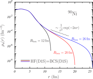
Figure 3: Neutron density distributions for the ⁹⁰Ni nucleus obtained in our HF(D1S)+BCS(D1S) calculations. Solid black, red and blue curves correspond, respectively, to $R_{\rm box}=12$, 20, and $26\,$fm. In all these calculations we have chosen $\epsilon_{\rm max}=10\,$MeV. The dashed straight line indicates the expected behavior of the density, according to Eq. (6).

In Fig. 3 we show the neutron density of the ⁹⁰Ni isotope calculated with HF(D1S)+BCS(D1S) for $R_{\rm box}$=12 (black curve), 20 (red curve) and 26 fm (blue curve). The dashed line indicates the expected asymptotic behavior

$$\rho_{\rm n}(r)\,\sim\,\displaystyle\frac{1}{r^{2}}\exp(-2\kappa r)\,,$$ (6)

where $\kappa=\sqrt{|E_{\rm min}-\lambda|2m_{\rm n}/\hbar^{2}}$. Here $E_{\rm min}=0.330\,$MeV is the value of the quasi-particle energy of the state defining the Fermi level for neutrons, the $2d_{3/2}$ in this case, and $\lambda=0.522\,$MeV is the BCS chemical potential. As it can be seen, this behavior is well reproduced at large $r$-values and no evidence of neutron gas effects is found.

III.2 Neutron rms radii and densities of Sn isotopes

Several Sn isotopes have been studied in the literature in connection with the neutron gas problem: abnormally high tails of their neutron densities Dobaczewski et al. (1996b) and huge growths of the neutron rms radii Dobaczewski et al. (1984); Ono et al. (2010) were considered as its signature.

We present in Table 3 the values of the rms radii of the neutron distributions corresponding to various even-even Sn isotopes, focussing on the convergence of the results in the three types of calculations that we have carried out. We have selected those Sn isotopes with spherical shape. The only exceptions are the ¹⁵⁰Sn and ¹⁶⁰Sn nuclei for which the HFB calculations of Ref. Hilaire and Girod indicate a small deformation. We have included them in our investigation because they have been specifically considered in the study of the neutron gas problem Dobaczewski et al. (1996b). In any case, we have carried out deformed HFB(D1S) calculations with the HFBAXIAL code and we have verified that the neutron rms radii values obtained for these two nuclei differ from those found in the spherical case by less than $0.04\%$.

		HF(D1S)+BCS(D1S)					HFB(D1S)					HFB(SLy5)
		$R_{\rm box}$ (fm)					$N_{\rm ho}$					$R_{\rm box}$ (fm)
nucleus		10	15	20	25		8	11	14	17		10	15	20	25
140Sn		4.93	4.98	4.98	4.98		4.97	4.97	4.99	4.99		5.00	5.05	5.05	5.05
142Sn		4.96	5.04	5.06	5.07		5.00	5.01	5.03	5.04		5.04	5.09	5.09	5.09
144Sn		5.02	5.04	5.04	5.04		5.04	5.05	5.07	5.08		5.07	5.13	5.13	5.13
146Sn		5.02	5.07	5.07	5.07		5.07	5.09	5.11	5.12		5.10	5.17	5.18	5.18
150Sn		5.10	5.24	5.28	5.30		5.14	5.16	5.18	5.20		5.17	5.25	5.25	5.26
160Sn		5.27	5.41	5.44	5.44		5.27	5.30	5.33	5.35		5.30	5.42	5.43	5.43
164Sn		5.31	5.45	5.48	5.49		5.31	5.35	5.38	5.41		5.35	5.47	5.49	5.49
166Sn		5.32	5.47	5.49	5.50		5.33	5.38	5.41	5.43		5.38	5.50	5.51	5.51
168Sn		5.34	5.48	5.50	5.51		5.35	5.40	5.43	5.45		5.40	5.52	5.53	5.53
170Sn		5.35	5.49	5.51	5.52		5.37	5.42	5.45	5.47		5.42	5.54	5.55	5.55
172Sn		5.36	5.50	5.52	5.52		5.39	5.44	5.47	5.49		5.44	5.56	5.57	5.57

Table 3: Neutron rms radii for various Sn isotopes calculated with HF(D1S)+BCS(D1S), with HFB(D1S), by using the HFBAXIAL code, and with HFB(SLy5), by using the HFBRAD code, approaches. The convergence with the corresponding values of $R_{\rm box}$ or $N_{\rm ho}$ is analyzed. The HF(D1S)+BCS(D1S) calculations have been carried out with $\epsilon_{\rm max}=10\,$MeV.

The results of Table 3 indicate the numerical stability of all our calculations for ${R_{\rm box}}$ values larger than 20 fm or $N_{\rm ho}$ larger than 14. In addition, the results obtained in the three approaches show a good agreement, with relative differences smaller than $2\%$. We do not observe any anomaly related to our HF(D1S)+BCS(D1S) results, which again do not show neutron gas effects.

Our results disagree with those of Ref. Dobaczewski et al. (1984) where it is shown that the neutron rms radii of the ¹²⁰Sn and ¹⁶⁰Sn nuclei grow with $R_{\rm box}$ in HF+BCS calculations, while remain almost constant in HFB. The relative differences between the results of the two calculations, carried out with $R_{\rm box}=25\,$fm, are about 6% and 20%, respectively, for the two Sn isotopes. Similar results are presented in Ref. Ono et al. (2010) where it is shown that the values of the neutron rms radii obtained in the HF+BCS approach grow with the increasing number of oscillator shells $N_{\rm ho}$ used in the calculation.

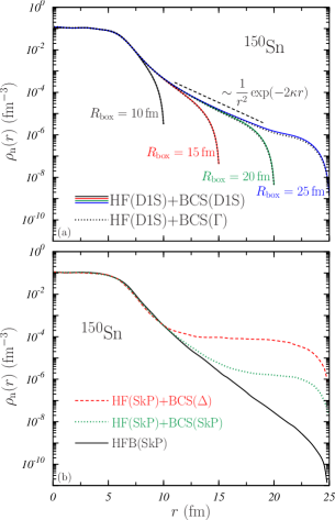
Figure 4: Neutron density distributions for the ¹⁵⁰Sn nucleus. In panel (a), the densities obtained in our HF(D1S)+BCS(D1S) calculations are shown by solid curves for $R_{\rm box}=10$ (black), 15 (red), 20 (green) and $25\,$fm (blue). The dotted black curves indicate the HF(D1S)+BCS($\Gamma$) results obtained for various $R_{\rm box}$ values. In all these calculations we have used $\epsilon_{\rm max}=10\,$MeV. The dashed straight line indicates the expected asymptotic behavior of the density, according to Eq. (6). In panel (b), we show the densities presented in Figs. 14 and 19 of Ref. Dobaczewski et al. (1996b). The HFB(SkP) density (solid black curve) is compared to those obtained in HF(SkP)+BCS($\Delta$) (dashed red curve) and HF(SkP)+BCS(SkP) (dotted green curve) calculations.

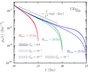
Figure 5: Neutron density distributions for the ¹⁵⁰Sn nucleus obtained in our HF(D1S)+BCS(D1S) calculations for $R_{\rm box}=15$ (red lines), 20 (green lines) and $25\,$fm (blue lines) by using $\epsilon_{\rm max}=10\,$MeV. Solid, dotted, dashed-dotted and dashed curves include all s.p. states with occupation probabilities $(v_{\alpha}^{\rm BCS})^{2}$ larger than 0, $10^{-4}$, $10^{-3}$ and $10^{-2}$, respectively. The dashed straight line indicates the expected asymptotic behavior of the density, according to Eq. (6).

We have analyzed the neutron density distributions of various Sn isotopes. As example of this investigation, we present in Fig. 4 the results obtained for ¹⁵⁰Sn, one of the isotopes studied in Ref. Dobaczewski et al. (1996b) to show the appearance of the neutron gas problem. The full lines in the panel (a) indicate the results of our HF(D1S)+BCS(D1S) calculations for different values of $R_{\rm box}$ from 10 to $25\,$fm. The dashed straight line shows the expected asymptotic behavior defined in Eq. (6), with $E_{\rm min}=0.561\,$MeV, corresponding to the neutron $3p_{1/2}$ s.p. level, and $\lambda=-0.304\,$MeV. This behavior is approximately reproduced at large $r$-values, independently of the ${R_{\rm box}}$ value. Our density distributions do not show any neutron gas effect.

The curves shown in panel (b) of Fig. 4 have been adapted from Figs. 14 and 19 of Ref. Dobaczewski et al. (1996b). They correspond to calculations that were carried out by using the Skyrme SkP interaction Dobaczewski et al. (1984). In comparison with the HFB(SkP) density (solid black line), the HF+BCS distributions (dashed red and dotted green curves) show large asymptotic tails that are extremely sensitive to the interaction used for the pairing field. The dotted green curve shows the result obtained when the SkP interaction is used consistently in both the HF and BCS parts of the calculation. If in the pairing channel the SkP force is substituted by a contact interaction with strength $\Delta$, the tail of the density distribution increases by more than one order of magnitude, as it is shown by the dashed red curve.

The results of Refs. Dobaczewski et al. (1984); Dobaczewski et al. (1996b) indicate a large sensitivity of the tails of the neutron density distributions to the interaction used in the BCS calculations. We have investigated if our results also show the same kind of sensitivity and if the neutron gas effects could appear when a zero-range interaction is utilized instead of a finite-range force. To clarify this point we have carried out BCS calculations with a $\delta-$contact interaction of the type

$$V({\bf r},{\bf r}^{\prime})\,=\,\Gamma\,\delta({\bf r}-{\bf r}^{\prime})$$ (7)

together with the HF(D1S) set of s.p. energies and wave functions. We have labelled HF(D1S)+BCS($\Gamma$) the corresponding results. The value of ${\epsilon_{\rm max}}$ is the same adopted in our usual HF(D1S)+BCS(D1S) calculations. The strength $\Gamma$ in Eq. (7) has been chosen to reproduce the average HF(D1S)+BCS(D1S) gap value,

$$\overline{\Delta}\,=\,\displaystyle\frac{\displaystyle\sum_{\alpha}\,(v_{\alpha}^{\rm BCS})^{2}\,\Delta_{\alpha}}{\displaystyle\sum_{\alpha}\,(v_{\alpha}^{\rm BCS})^{2}}\,.$$ (8)

In the previous equation $\Delta_{\alpha}$ indicates the BCS gap of the corresponding quasiparticle state.

The results of these calculations are shown in the panel (a) of Fig. 4 by the dotted black curves. These density distributions are very similar to the HF(D1S)+BCS(D1S) ones and do not show any indication of the presence of the neutron gas. This is also confirmed by the fact that the values of the neutron rms radii differ from those given in Table 3 by less than 0.1% , at maximum, which is the case of $R_{\rm box}=25\,$fm. We have obtained similar results for all the Sn isotopes investigated.

A careful observation of Fig. 4(a) indicates that the density obtained with $R_{\textrm{box}}=25\,$fm has a small hump in the region above $20\,$fm. To understand the source of this behavior, we have studied the relative importance of the s.p. states contributing to this density distribution, i. e. to the diagonal part of the OBDM defined in Eq. (4). As each s.p. wave function is weighted by its occupation probability $(v^{\textrm{BCS}}_{\alpha})^{2}$, we have surmised that the hump could be generated by the presence of s.p. states with very small occupation probabilities. For this reason, we have calculated the density distribution by selecting s.p. states with $(v^{\textrm{BCS}}_{\alpha})^{2}>v_{\rm cut}^{2}$.

The results of this study are presented in Fig. 5 where the densities obtained with $v_{\rm cut}^{2}=10^{-4}$ (dotted lines), $v_{\rm cut}^{2}=10^{-3}$ (dashed dotted lines) and $v_{\rm cut}^{2}=10^{-2}$ (dashed lines) are compared with those of Fig 4(a), which correspond to $v_{\rm cut}^{2}=0$ (full lines). These results indicate that the hump at large $r$ values is clearly due to the contribution of s.p. states with very small occupation probabilities. The effect becomes larger with increasing $R_{\textrm{box}}$, as it is evident for the results corresponding to $R_{\textrm{box}}=25\,$fm. It is also worth pointing out that, in this case, the densities obtained with $v_{\rm cut}^{2}=10^{-3}$ or $10^{-2}$ verify much better the expected asymptotic behavior indicated in the figure by the black dashed straight line.

We have further investigated the relevance of the s.p. states with small occupation probabilities, by comparing our HF(D1S)+BCS(D1S) calculations for different values of $v_{\rm cut}^{2}$ with the HFB(SLy5) results obtained by using the HFBRAD code. In order to make a fair comparison we have renormalized our HF(D1S)+BCS(D1S) density distributions to the correct number of nucleons. In all cases, $R_{\textrm{box}}=25\,$fm has been considered.

Figure 6: Ratios between the neutron densities generated by our HF(D1S)+BCS(D1S) calculations, with $R_{\rm box}=25$ and $\epsilon_{\rm max}=10\,$MeV, and that obtained in a HFB(SLy5) calculation carried out with HFBRAD. Solid, dotted, dashed-dotted and dashed curves include, in the HF+BCS calculations, all s.p. states with occupation probabilities $(v_{\alpha}^{\rm BCS})^{2}$ larger than 0, $10^{-4}$, $10^{-3}$ and $10^{-2}$, respectively. The neutron rms radii obtained in the HF(D1S)+BCS(D1S) calculations are given in the inset.

In Fig. 6 we show the ratio between the HF(D1S)+BCS(D1S) densities, obtained by using the prescription above described for different values of $v_{\rm cut}^{2}$, and that of the HFB(SLy5) calculation. These ratios remain close to 1 up to about $15\,$fm and grow for larger $r$ values. The strong reduction of the ratio observed for $r\geq 20\,$fm when $v^{2}_{\rm cut}=10^{-2}$ and $10^{-3}$, shows the relevance of s.p. states with small occupation probability. In the inset of the figure, we also present the values of the corresponding neutron rms radii, which coincide with those obtained before the renormalisation of the densities. The relative difference among these values is $0.2\%$ at most, similar to the differences found between the neutron rms radii shown in Table 3. It is worth mentioning that the results obtained for the rms neutron radii of some Sn isotopes by Del Estal et al. in a BCS calculation, considering all s.p. states with positive energies or just those corresponding to quasi-bound states show the same relative differences Del Estal et al. (2001).

III.3 Proton elastic cross sections

The results we have discussed so far indicate that our HF+BCS calculations do not show the large neutron gas effects mentioned in Refs. Dobaczewski et al. (1984); Dobaczewski et al. (1996a, b); Dobaczewski (1999); Ono et al. (2010). On the other hand, we have found that at large $r$ values, s.p. states with small occupation probability slightly modify the expected behavior of the density distributions. Slightly means that these modifications are several order of magnitude smaller than the maximum values of the distributions, and in the figures we emphasize them by using a logarithmic scale. In this section we investigate the relevance of these modifications of the neutron density distributions at large $r$ values in the calculations of other observables.

A first answer to this question is already provided by the results of Table 3 showing that the neutron rms radii are extremely stable against the increase of the $R_{\textrm{box}}$ values. This means that the s.p. states generating the small hump observed at large $r$ are irrelevant in the calculation of these radii.

We have also studied the possible effects of these states on the differential cross section for proton elastic scattering off ¹⁵⁰Sn. We have chosen this nucleus since, in Ref. Dobaczewski et al. (1996b), shows large neutron gas effects. The calculations of the cross sections have been done by adopting a rather simple optical potential generated by folding the corresponding total matter density, i. e. the sum of the proton and neutron densities, with a contact nucleon-nucleon potential:

$$V({\bf r},{\bf r}^{\prime})\,=\,-V_{0}\,\delta({\bf r}-{\bf r}^{\prime})\,.$$ (9)

We have chosen the strength value as $V_{0}=50\,$MeV.

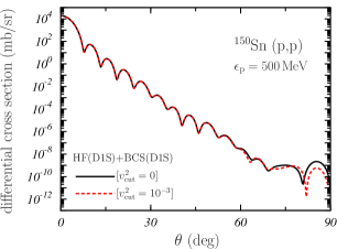
Figure 7: Differential cross sections for elastic scattering of $500\,$MeV protons off ¹⁵⁰Sn nucleus. The optical potential used in the calculations has been obtained by folding the nucleon-nucleon potential defined in Eq. (9) with the matter densities generated in our HF(D1S)+BCS(D1S) approach, with $R_{\rm box}=25\,$fm and $\epsilon_{\rm max}=10\,$MeV. The solid black curve has been obtained with a matter density calculated by considering all the BCS s.p. states, while the dashed red curve shows the results obtained by using a, renormalized, matter density where only the s.p. states with BCS occupation $(v_{\alpha}^{\rm BCS})^{2}>10^{-3}$ have been taken into account.

The results obtained are shown in Fig. 7 for a proton incident energy of $500\,$MeV. In this calculation the matter densities have been obtained by using the s.p. wave functions obtained in our HF(D1S)+BCS(D1S) with ${R_{\rm box}}=25\,$fm and ${\epsilon_{\rm max}}=10\,$MeV. The solid black line indicates the result obtained by considering the full set of BCS s.p. wave functions, while the dashed red curve that obtained by considering $v^{2}_{\textrm{cut}}>10^{-3}$, and, of course, properly renormalizing the density. The two curves are almost overlapping up to a scattering angle of about $60\,$degrees. Some differences occur above this value where the differential cross section is 14 order of magnitude smaller than the maximum obtained at $\theta=0$. We have checked that, for incident energies smaller than 400 MeV, the corresponding curves overlap up to $90\,$degrees.

IV Summary and conclusions

From the theoretical point of view, BCS calculations are affected by neutron gas effects that are instead absent, by construction, in the HFB approach. These effects are due to the s.p. states with positive energies and we have studied their quantitative relevance by comparing the results of HF+BCS and HFB calculations carried out with various interactions and different numerical techniques.

We have not found any remarkable evidence of the neutron gas problem in all the observables analyzed. The contribution of the largest part of the s.p. states with positive energy is quantitatively irrelevant due to the fact that their occupation probabilities are very small.

We have also excluded that the use of a zero-range interaction in the pairing sector could enhance the effect of the neutron gas.

We have pointed out that a proper choice of the input parameters ensures a good numerical convergence of the values of the neutron rms radii.

We have investigated the role of the s.p. states with small occupation probabilities in the neutron density distributions and we have found that they produce a small hump at large distances from the nuclear center. This effect is due to accumulated contributions of a large number of these s.p. states. This enhancement in the density is, however, orders of magnitude smaller than those claimed in the literature as a neutron gas evidence.

These results indicate the reliability of the HF+BCS approach in the description of nuclei with large neutron excess.