Abstract

An integrable semi-discretization of complex and multi-component coupled dispersionless systems via Lax pairs is presented. A Lax pair is proposed for the complex sdCD system. We derive the Lax pair for the multi-component sdCD system through generalizing the $2\times 2$ Lax matrices to the case of $2^{N}\times 2^{N}$ Lax matrices. A Darboux transformation (DT) is applied to the complex and multi-component sdCD systems and is used to compute soliton solutions of the systems. It is also shown that the soliton solutions of the semi-discrete systems reduce to the continuous systems by applying continuum limit.

PACS: 02.30.Ik, 05.45.Yv
Keywords: Discrete Integrable systems, solitons, Darboux transformation

1 Introduction

Integrable discrete nonlinear equations defined on a lattice points rather than a continuum space-time, play an important role in the field of applied mathematics and nonlinear science. Generically, they admit many solutions known as soliton solutions. Due to solitonic behavior, integrable discrete systems become very compelling from a physical point of view. Such systems are not only useful in the study of numerical scheme but they also serve as physical models in which space-coordinates are defined on lattice points and time is taken as continuous. Examples are found in various disciplines of science such as nonlinear lattices, plasma physics, statistical mechanics and optical fibers etc. [1]-[7].

In the last couple of decades, dispersionless or quasiclassical limits of integrable equations and hierarchies have received much attention by researchers since they arise in the analysis of several problems in applied mathematics and physics from the theory of quantum fields and conformal maps on the complex plane [8]-[17]. In [15], some authors proposed a set of coupled dispersionless (CD) integrable system given by

$$\partial_{x}\partial_{t}q+2\partial_{x}rr = 0,$$ (1.1)

$$\partial_{x}\partial_{t}r-2\partial_{x}qr = 0.$$ (1.2)

where $q\equiv q(x,\;t)$ and $r\equiv r(x,\;t)$ are real functions of $x$ and $t$. The system (1.1)-(1.2) is called dispersionless because of not containing the dispersion term rather than arising as a semi-classical limit. A generalized version of the CD system was introduced by the same authors [16] and is given by

$$\partial_{x}\partial_{t}q+\partial_{x}(rs) = 0,$$ (1.3)

$$\partial_{x}\partial_{t}r-2\partial_{x}qr = 0,$$ (1.4)

$$\partial_{x}\partial_{t}s-2\partial_{x}qs = 0,$$ (1.5)

where $s\equiv s(x,t)$ is a real function of $x$ and $t$. The inverse scheme of the set of equations (1.3)-(1.5) is given by

$$\partial_{x}\Psi = U\Psi=-\dot{\imath}\lambda^{-1}\left(\begin{array}[]{cc}\partial_{x}q&\partial_{x}r\\ \partial_{x}s&-\partial_{x}q\end{array}\right)\Psi,$$ (1.8)

$$\partial_{t}\Psi = V\Psi=\left[\left(\begin{array}[]{cc}0&-r\\ s&0\end{array}\right)+\dot{\imath}\lambda\left(\begin{array}[]{cc}\frac{1}{2}&0\\ 0&-\frac{1}{2}\end{array}\right)\right]\Psi.$$ (1.13)

For $s=\bar{r}$ (where $\bar{r}$ represent complex conjugate of $r$), we get the complex CD system [17]. Physically CD system describes the interaction of current-fed string in a certain external magnetic field. CD system and complex CD system have been shown to be gauge equivalent to the sine-Gordon equation and Pohlmeyer-Lund-Regge model [18], [19]. Most recently, the link of the motion of space curves to the real and complex CD system and to the real and complex short-pulse equations has been established via hodograph transformation. Further, the connection is shown to be made clear between the real (complex) CD system and real (complex) short-pulse equations and also with the two-component Kadomtsew-Petviashvili (KP) hierarchy [20]. In past years, the CD and complex CD systems, their generalization to a system based on non-abelian Lie group and its non-commutative extension have been studied and proved to be completely solvable by inverse scattering method, Darboux transformation and with the help of other methods of generating solutions [15]-[17], [21]-[24].

Along with continuous coupled dispersionless system, its discrete version also preserves the integrability of the system. In [25]-[26], Vinet and Yu presented a discretization of the CD and generalized CD system and obtained soliton solutions via Hirota bilinear method. In [27]-[29], Darboux transformations are used to discretize the CD system and their generalizations. Meanwhile the behavior of soliton solutions have also been investigated. In the present work, we present a semi-discretization of the complex CD system via Lax pair. We shall also study an integrable semi-discritization of multi-component generalization of the complex CD system

$$\partial_{x}\partial_{t}q+\partial_{x}\left(\sum_{j=1}^{N}|r^{(j)}|^{2}\right)=0,$$ (1.14)

$$\partial_{x}\partial_{t}r^{(j)}-2qr^{(j)}=0,\quad j=1,\;2,\;3,\;...,\;N.$$ (1.15)

The multi-component complex CD system (1.14)-(1.15) proposed in [30] and the soliton solutions were investigated by means of Hirota bilinear method.

The paper is structured as follows. In section 2, we present an integrable semi-discretization of the complex CD system via Lax representation. We then extend the $2\times 2$ Lax matrices for the case of $2^{N}\times 2^{N}$ Lax matrices and obtain a multi-component generalization of sdCD system. We also reduce both complex sdCD and multi-component sdCD system to their respective continuous counterparts by applying continuum limit. In section 3, we define Darboux transformation (DT) for the multi-component complex sdCD system and obtain multisoliton solutions. Further, we present quasideterminant solutions of the multi-component sdCD system. In section 4, we present soliton solutions for the complex and 2-component complex sdCD system.

2 Lax pair representation

We start with the Lax pair of the complex sdCD system which is a set of differential-difference equations where space is taken as one dimensional lattice and time is taken as continuous given by

$$\Psi_{n+1} = \mathcal{L}_{n}\Psi_{n}=\left(\begin{array}[]{cc}1-\dot{\imath}\lambda^{-1}(q_{n+1}-q_{n})&-\dot{\imath}\lambda^{-1}(r_{n+1}-r_{n})\\ -\dot{\imath}\lambda^{-1}(\bar{r}_{n+1}-\bar{r}_{n})&1+\dot{\imath}\lambda^{-1}(q_{n+1}-q_{n})\end{array}\right),$$ (2.3)

$$\frac{d}{dt}\Psi_{n} = \mathcal{M}_{n}\Psi_{n}=\left(\begin{array}[]{cc}\frac{\dot{\imath}\lambda}{2}&-r_{n}\\ \bar{r}_{n}&-\frac{\dot{\imath}\lambda}{2}\end{array}\right),$$ (2.6)

where $n$ represents discrete index and $\bar{r}_{n}$ represents the complex conjugate of $r_{n}$ and $\lambda$ is a spectral parameter. The zero-curvature condition $\frac{d}{dt}\mathcal{L}_{n}+\mathcal{L}_{n}\mathcal{M}_{n}-\mathcal{M}_{n+1}\mathcal{L}_{n}=0$ yields the complex sdCD system

$$\frac{d}{dt}(q_{n+1}-q_{n})+\left(\left|r_{n+1}\right|^{2}-\left|r_{n}\right|^{2}\right) = 0,$$ (2.7)

$$\frac{d}{dt}(r_{n+1}-r_{n})-(r_{n+1}+r_{n})(q_{n+1}-q_{n}) = 0.$$ (2.8)

The Lax pair for the multi-component generalization of the complex sdCD system is obtained by extending the $2\times 2$ Lax pair matrices to the case of $2^{N}\times 2^{N}$ Lax matrices. The Lax pair for the multi-component sdCD system is expressed as

$$\Psi_{n+1} = \mathcal{L}_{n}\Psi_{n}=\left(\mathcal{J}+\lambda^{-1}(\mathcal{U}_{n+1}-\mathcal{U}_{n})\right)\Psi_{n},$$ (2.9)

$$\frac{d}{dt}\Psi_{n} = \mathcal{M}_{n}\Psi_{n}=\left(\mathcal{V}_{n}+\lambda\mathcal{V}_{0}\right)\Psi_{n},$$ (2.10)

where $\mathcal{J},\;\mathcal{U}_{n},\;\mathcal{V}_{n}$ and $\mathcal{V}_{0}$ are the $2^{N}\times 2^{N}$ block matrices given by

$$\mathcal{J}=\left(\begin{array}[]{cc}I&O\\ O&I\end{array}\right),\quad\mathcal{U}_{n}=-\dot{\imath}\left(\begin{array}[]{cc}\mathcal{Q}_{n}&\mathcal{R}_{n}\\ \mathcal{S}_{n}&-\mathcal{Q}_{n}\end{array}\right),\quad\mathcal{V}_{n}=\left(\begin{array}[]{cc}O&-\mathcal{R}_{n}\\ \mathcal{S}_{n}&O\end{array}\right),\quad\mathcal{V}_{0}=\left(\begin{array}[]{cc}\frac{\dot{\imath}}{2}I&O\\ O&-\frac{\dot{\imath}}{2}I\end{array}\right),$$ (2.11)

where $\mathcal{Q}_{n},\mathcal{R}_{n}$ and $\mathcal{S}_{n}=\mathcal{R}_{n}^{{\dagger}}$ (here ${\dagger}$ in the superscript denotes Hermitian conjugation) are the $2^{N-1}\times 2^{N-1}$ block matrices and $O,\;I$ are the $2^{N-1}\times 2^{N-1}$ null and unit matrices, respectively. The compatibility condition of the Lax pair (2.9)-(2.10) gives the matrix complex sdCD system

$$\frac{d}{dt}(\mathcal{U}_{n+1}-\mathcal{U}_{n})+(\mathcal{U}_{n+1}-\mathcal{U}_{n})\mathcal{V}_{n}-\mathcal{V}_{n+1}(\mathcal{U}_{n+1}-\mathcal{U}_{n})=O.$$ (2.12)

By substituting the expression of $\mathcal{U}_{n}$ and $\mathcal{V}_{n}$ from (2.11) into (2.12), we obtain

$$\frac{d}{dt}(\mathcal{Q}_{n+1}-\mathcal{Q}_{n})+\mathcal{R}_{n+1}\mathcal{S}_{n+1}-\mathcal{R}_{n}\mathcal{S}_{n} = O,$$ (2.13)

$$\frac{d}{dt}(\mathcal{R}_{n+1}-\mathcal{R}_{n})-(\mathcal{Q}_{n+1}-\mathcal{Q}_{n})\mathcal{R}_{n}-\mathcal{R}_{n+1}(\mathcal{Q}_{n+1}-\mathcal{Q}_{n}) = O.$$ (2.14)

In the case, where we define the matrix variables $\mathcal{Q}_{n},\;\mathcal{R}_{n}$ in terms of scalar dependent variables $q_{n},\;r_{n}$, i.e. $\mathcal{Q}_{n}\equiv q_{n},\;\mathcal{R}_{n}\equiv r_{n}$, one can reduce the matrix complex sdCD system (2.13)-(2.14) to the complex sdCD system (2.7)-(2.8), and when the matrices $\mathcal{Q}_{n}$ and $\mathcal{R}_{n}$ take the form

$$\mathcal{Q}_{n}^{(2)}=q_{n}I_{2\times 2},\quad{\mathcal{R}_{n}^{(2)}}=\left(\begin{array}[]{c:c}r_{n}^{(1)}&r_{n}^{(2)}\\ \hdashline-\bar{r}_{n}^{(2)}&\bar{r}_{n}^{(1)}\end{array}\right)_{2\times 2},$$ (2.17)

$$\mathcal{Q}_{n}^{(3)}=q_{n}I_{4\times 4},\quad\mathcal{R}_{n}^{(3)}=\left(\begin{array}[]{c:c}\begin{array}[]{cc}r_{n}^{(1)}&r_{n}^{(2)}\\ -\bar{r}_{n}^{(2)}&\bar{r}_{n}^{(1)}\end{array}&\begin{array}[]{cc}r_{n}^{(3)}&0\\ 0&r_{n}^{(3)}\end{array}\\ \hdashline\begin{array}[]{cc}-\bar{r}_{n}^{(3)}&0\\ 0&-\bar{r}_{n}^{(3)}\end{array}&\begin{array}[]{cc}\bar{r}_{n}^{(1)}&-r_{n}^{(2)}\\ \bar{r}_{n}^{(2)}&r_{n}^{(1)}\end{array}\end{array}\right)_{4\times 4},$$ (2.28)

$$\mathcal{Q}_{n}^{(4)}=q_{n}I_{8\times 8},$$ (2.29)

$$\mathcal{R}_{n}^{(4)}=\left(\begin{array}[]{c:c}\begin{array}[]{cccc}r_{n}^{(1)}&r_{n}^{(2)}&0&0\\ -\bar{r}_{n}^{(2)}&\bar{r}_{n}^{(1)}&0&0\\ 0&0&r_{n}^{(1)}&r_{n}^{(2)}\\ 0&0&-\bar{r}_{n}^{(2)}&\bar{r}_{n}^{(1)}\end{array}&\begin{array}[]{cccc}r_{n}^{(3)}&0&r_{n}^{(4)}&0\\ 0&r_{n}^{(3)}&0&r_{n}^{(4)}\\ -\bar{r}_{n}^{(4)}&0&\bar{r}_{n}^{(3)}&0\\ 0&-\bar{r}_{n}^{(4)}&0&\bar{r}_{n}^{(3)}\end{array}\\ \hdashline\begin{array}[]{cccc}-\bar{r}_{n}^{(3)}&0&r_{n}^{(4)}&0\\ 0&-\bar{r}_{n}^{(3)}&0&r_{n}^{(4)}\\ -\bar{r}_{n}^{(4)}&0&-r_{n}^{(3)}&0\\ 0&-\bar{r}_{n}^{(4)}&0&-r_{n}^{(3)}\end{array}&\begin{array}[]{cccc}\bar{r}_{n}^{(1)}&-r_{n}^{(2)}&0&0\\ \bar{r}_{n}^{(2)}&r_{n}^{(1)}&0&0\\ 0&0&\bar{r}_{n}^{(1)}&-r_{n}^{(2)}\\ 0&0&\bar{r}_{n}^{(2)}&r_{n}^{(1)}\end{array}\end{array}\right)_{8\times 8},$$ (2.48)

we get multi-component complex sdCD system. By substituting the expressions of (2.17)-(2.29) into the set of equations (2.13)-(2.14), we obtain respectively, the 2-component, 3-component and 4-component complex sdCD system. The 2-component complex sdCD is

$$\frac{d}{dt}(q_{n+1}-q_{n})+\sum_{j=1}^{2}\left(|r_{n+1}^{(j)}|^{2}-|r_{n}^{(j)}|^{2}\right)=0,$$ (2.49)

$$\frac{d}{dt}(r_{n+1}^{(j)}-r_{n}^{(j)})-(r_{n+1}^{(j)}+r_{n}^{(j)})(q_{n+1}-q_{n})=0,\quad j=1,\;2.$$ (2.50)

The 3-component complex sdCD system is

$$\frac{d}{dt}(q_{n+1}-q_{n})+\sum_{j=1}^{3}\left(|r_{n+1}^{(j)}|^{2}-|r_{n}^{(j)}|^{2}\right)=0,$$ (2.51)

$$\frac{d}{dt}(r_{n+1}^{(j)}-r_{n}^{(j)})-(r_{n+1}^{(j)}+r_{n}^{(j)})(q_{n+1}-q_{n})=0,\quad j=1,\;2,\;3.$$ (2.52)

Similarly, $N$-component complex sdCD system is given by

$$\frac{d}{dt}(q_{n+1}-q_{n})+\sum_{j=1}^{N}\left(|r_{n+1}^{(j)}|^{2}-|r_{n}^{(j)}|^{2}\right)=0,$$ (2.53)

$$\frac{d}{dt}(r_{n+1}^{(j)}-r_{n}^{(j)})-(r_{n+1}^{(j)}+r_{n}^{(j)})(q_{n+1}-q_{n})=0,\quad j=1,\;...,\;N.$$ (2.54)

In general, the expressions of the $2^{N-1}\times 2^{N-1}$ matrices $\mathcal{Q}_{n}^{(N)}$ and $\mathcal{R}_{n}^{(N)}$ are

$$\mathcal{Q}_{n}^{(N)}=q_{n}I_{2^{N-1}\times 2^{N-1}},\quad\mathcal{R}_{n}^{(N)}=\left(\begin{array}[]{c:c}\mathbb{R}_{n}^{(1)}&\mathbb{R}_{n}^{(2)}\\ \hdashline\mathbb{R}_{n}^{(3)}&\mathbb{R}_{n}^{(4)}\end{array}\right),$$ (2.57)

where $\mathbb{R}_{n}^{(j)}$ ($j=1,\;2,\;3,\;4$) are all $2^{N-2}\times 2^{N-2}$ square block matrices, and $\mathbb{R}_{n}^{(4)}=(\mathbb{R}_{n}^{(1)})^{{\dagger}},\;\mathbb{R}_{n}^{(3)}=-(\mathbb{R}_{n}^{(2)})^{{\dagger}}$. The matrices $\mathbb{R}_{n}^{(1)}$ and $\mathbb{R}_{n}^{(2)}$ are given by

$$\mathbb{R}_{n}^{(1)}=\left(\begin{array}[]{ccccc}\mathbb{X}_{n}^{(1)}&&&\text{\Huge O}&\\ &\mathbb{X}_{n}^{(1)}&&&\\ &&\ddots&&\\ &&&\mathbb{X}_{n}^{(1)}&\\ &\text{\Huge O}&&&\mathbb{X}_{n}^{(1)}\end{array}\right),\quad\mathbb{R}_{n}^{(2)}=\left(\begin{array}[]{c:c}\mathbb{Y}_{n}^{(1)}&\mathbb{Y}_{n}^{(2)}\\ \hdashline\mathbb{Y}_{n}^{(3)}&\mathbb{Y}_{n}^{(4)}\end{array}\right),$$ (2.58)

where $\mathbb{Y}_{n}^{(4)}=(\mathbb{Y}_{n}^{(1)})^{{\dagger}},\;\mathbb{Y}_{n}^{(3)}=-(\mathbb{Y}_{n}^{(2)})^{{\dagger}}$ are all square block matrices which take values in the following form

$$\mathbb{Y}_{n}^{(1)}=\left(\begin{array}[]{cccc}\mathbb{X}_{n}^{(2)}&&&\text{\Huge O}\\ &\mathbb{X}_{n}^{(2)}&&\\ &&\ddots&\\ \text{\Huge O}&&&\mathbb{X}_{n}^{(2)}\end{array}\right),\;\mathbb{Y}_{n}^{(2)}=\left(\begin{array}[]{ccccc}\mathbb{X}_{n}^{(3)}&\mathbb{O}&\ldots&\mathbb{X}_{n}^{(N-1)}&\mathbb{X}_{n}^{(N)}\\ \mathbb{O}&\mathbb{X}_{n}^{(3)}&\ldots&-\mathbb{X}_{n}^{(N)}&\mathbb{X}_{n}^{(N-1)}\\ \vdots&\vdots&\ddots&\vdots&\vdots\\ -\mathbb{X}_{n}^{(N-1)}&\mathbb{X}_{n}^{(N)}&\ldots&\mathbb{X}_{n}^{(3)}&\mathbb{O}\\ -\mathbb{X}_{n}^{(N)}&-\mathbb{X}_{n}^{(N-1)}&\ldots&\mathbb{O}&\mathbb{X}_{n}^{(3)}\end{array}\right),$$ (2.68)

$$\mathbb{O}=\left(\begin{array}[]{cc}0&0\\ 0&0\end{array}\right),\quad\mathbb{X}_{n}^{(1)}=\left(\begin{array}[]{cc}r_{n}^{(1)}&r_{n}^{(2)}\\ -\bar{r}_{n}^{(2)}&\bar{r}_{n}^{(1)}\end{array}\right),\quad\mathbb{X}_{n}^{(j)}=\left(\begin{array}[]{cc}r_{n}^{(j+1)}&0\\ 0&r_{n}^{(j+1)}\end{array}\right),$$ (2.75)

$$\qquad\qquad\qquad\qquad\qquad\qquad\qquad\qquad\qquad\qquad\qquad j=2,\;3,\;...,\;N-1.$$ (2.76)

Substituting (2.57) and (2.76) into the set of equations (2.13)-(2.14), we obtain $N$-component complex sdCD system (2.53)-(2.54). Equations (2.7)-(2.8) and (2.53)-(2.54) represents respectively, an integrable semi-discrete (discrete in space-coordinate) analogue of the complex and multi-component complex sdCD system. They can be reduced to the continuous complex and multi-component complex CD systems by applying continuum limit. For this, let us define $\lim_{\delta\rightarrow 0}\frac{f_{n+1}-f_{n}}{\delta}=f_{x}$, where $\delta$ is the lattice parameter in space-direction. Applying this to equations (2.53)-(2.54), one can obtain multi-component complex CD system given by

$$\partial_{x}\partial_{t}q+\partial_{x}\left(\sum_{j=1}^{N}|r^{(j)}|^{2}\right)=0,$$ (2.77)

$$\partial_{x}\partial_{t}r^{(j)}-2qr^{(j)}=0,\quad j=1,\;2,\;3,\;...,\;N.$$ (2.78)

For $N=1$, the set of equations (2.77)-(2.78) reduce to the usual complex CD system

$$\partial_{x}\partial_{t}q+\partial_{x}|r|^{2}=0,$$ (2.79)

$$\partial_{x}\partial_{t}r-2qr=0.$$ (2.80)

3 Darboux transformation

Darboux transformation (DT) is one of solution generating technique in soliton theory that allow us to express the solutions for a given integrable equation in simple explicit form [32]-[37]. In this section, we construct the DT of the multi-component complex sdCD system (2.13)-(2.14).

In what follows, we shall apply a DT to the solutions of the Lax pair and the solutions of the multi-component complex sdCD system and then express in terms of quasideterminents. Let us define a new solution $\Psi_{n}^{[1]}$ to the Lax pair (2.9)-(2.10) which is related to the old solution $\Psi_{n}$ by means of $2^{N}\times 2^{N}$ matrix $\mathcal{D}_{n}(t;\;\lambda)$ called the Darboux matrix. The one-fold DT on the solution to the Lax pair is given by

$$\Psi_{n}^{[1]}=\mathcal{D}_{n}(t;\;\lambda)\Psi_{n}=\left(\lambda\mathcal{I}-\Xi_{n}\right)\Psi_{n}.$$ (3.1)

In the present case, $\mathcal{I}$ is a $2^{N}\times 2^{N}$ unit matrix and $\Xi_{n}$ is an invertible $2^{N}\times 2^{N}$ matrix, to be determined. The new solution $\Psi_{n}^{[1]}$ satisfies the same Lax pair i.e.

$$\Psi_{n+1}^{[1]} = \mathcal{L}_{n}^{[1]}\Psi_{n}^{[1]}=\left(\mathcal{J}^{[1]}+\lambda^{-1}(\mathcal{U}_{n+1}^{[1]}-\mathcal{U}_{n}^{[1]})\right)\Psi_{n}^{[1]},$$ (3.2)

$$\frac{d}{dt}\Psi_{n}^{[1]} = \mathcal{M}_{n}^{[1]}\Psi_{n}^{[1]}=\left(\mathcal{V}_{n}^{[1]}+\lambda\mathcal{V}_{0}^{[1]}\right)\Psi_{n}^{[1]}.$$ (3.3)

By substituting the expression of $\Psi_{n}^{[1]}$ from (3.1) into Lax pair equations (3.2)-(3.3), we obtain DT on the matrices $\mathcal{U}_{n},\;\mathcal{V}_{n},\;\mathcal{J}$ and $\mathcal{V}_{0}$

$$\mathcal{U}_{n}^{[1]} = \mathcal{U}_{n}-\Xi_{n},$$ (3.4)

$$\mathcal{V}_{n}^{[1]} = \mathcal{V}_{n}+\left[\mathcal{V}_{0},\;\Xi_{n}\right],$$ (3.5)

$$\mathcal{J}^{[1]} = \mathcal{J},\quad\mathcal{V}_{0}^{[1]}=\mathcal{V}_{0},$$ (3.6)

with the conditions on the matrix $\Xi_{n}$ arising due to the Darboux covariance as follows

$$\left(\Xi_{n+1}-\Xi_{n}\right)\Xi_{n} = \left(\mathcal{U}_{n+1}-\mathcal{U}_{n}\right)\Xi_{n}-\Xi_{n+1}\left(\mathcal{U}_{n+1}-\mathcal{U}_{n}\right),$$ (3.7)

$$\frac{d}{dt}\Xi_{n} = \left[\mathcal{V}_{n},\;\Xi_{n}\right]+\left[\mathcal{V}_{0},\;\Xi_{n}\right]\Xi_{n}.$$ (3.8)

Now we construct the matrix $\Xi_{n}$ in terms of solutions to the Lax pair (2.9)-(2.10). For this we proceed as follows:

Define $2^{N}$ distinct constant parameters $\lambda_{1},\;\lambda_{2},\;...,\;\lambda_{2^{N}}$ such that for each $\lambda_{j}$ we have a peculiar column vector solution $\left|f^{(j)}\right\rangle_{n}=\Psi(\lambda_{j})\left|e_{j}\right\rangle$ (where $\left|e_{j}\right\rangle$ is a constant column vector) to the Lax pair (2.9)-(2.10). For $\lambda=\lambda_{j}$ ($j=1,\;2,\;...,\;2^{N}$), we write

$$\left|f^{(j)}\right\rangle_{n+1} = \left|f^{(j)}\right\rangle_{n}+\lambda^{-1}_{j}\left(\mathcal{U}_{n+1}-\mathcal{U}_{n}\right)\left|f^{(j)}\right\rangle_{n},$$ (3.9)

$$\frac{d}{dt}\left|f^{(j)}\right\rangle_{n} = \mathcal{V}_{n}\left|f^{(j)}\right\rangle_{n}+\lambda_{j}\mathcal{V}_{0}\left|f^{(j)}\right\rangle_{n}.$$ (3.10)

Define $2^{N}\times 2^{N}$ constant eigenvalue matrix with entries $\lambda_{j}$ i.e. $\Lambda=\text{diag}(\lambda_{1},\;...,\;\lambda_{2^{N}})$, and construct an invertible $2^{N}\times 2^{N}$ matrix $\mathcal{F}_{n}$ as

$$\mathcal{F}_{n}=\left(\Psi_{n}(\lambda_{1})\left|e_{1}\right\rangle,\;...,\;\Psi_{n}(\lambda_{2^{N}})\left|e_{2^{N}}\right\rangle\right)=\left(\left|f^{(1)}\right\rangle_{n},\;...,\;|f^{(2^{N})}\rangle_{n}\right),$$ (3.11)

so that the Lax pair (2.9)-(2.10) with the particular matrix $\mathcal{F}_{n}$ as solution, can be written as

$$\mathcal{F}_{n+1} = \mathcal{F}_{n}+\left(\mathcal{U}_{n+1}-\mathcal{U}_{n}\right)\mathcal{F}_{n}\Lambda^{-1},$$ (3.12)

$$\frac{d}{dt}\mathcal{F}_{n} = \mathcal{V}_{n}\mathcal{F}_{n}+\mathcal{V}_{0}\mathcal{F}_{n}\Lambda.$$ (3.13)

Further we check that the choice of the matrix $\Xi_{n}=\mathcal{F}_{n}\Lambda\mathcal{F}_{n}^{-1}$ satisfy the conditions (3.7)-(3.8) as imposed by Darboux covariance. This can be checked by a direct computation as follows

$$\left(\Xi_{n+1}-\Xi_{n}\right)\Xi_{n} = \mathcal{F}_{n+1}\Lambda\mathcal{F}_{n+1}^{-1}\mathcal{F}_{n}\Lambda\mathcal{F}_{n}^{-1}-\mathcal{F}_{n}\Lambda\mathcal{F}_{n}^{-1}\mathcal{F}_{n}\Lambda\mathcal{F}_{n}^{-1}$$ (3.14)

$$+ \mathcal{F}_{n+1}\Lambda\mathcal{F}_{n}^{-1}\mathcal{F}_{n}\Lambda\mathcal{F}_{n}^{-1}-\mathcal{F}_{n+1}\Lambda\mathcal{F}_{n+1}^{-1}\mathcal{F}_{n+1}\Lambda\mathcal{F}_{n}^{-1},$$

$$= \left(\mathcal{F}_{n+1}\Lambda\mathcal{F}_{n}^{-1}-\mathcal{F}_{n}\Lambda\mathcal{F}_{n}^{-1}\right)\mathcal{F}_{n}\Lambda\mathcal{F}_{n}^{-1}-\mathcal{F}_{n+1}\Lambda\mathcal{F}_{n+1}^{-1}\left(\mathcal{F}_{n+1}\Lambda\mathcal{F}_{n}^{-1}-\mathcal{F}_{n}\Lambda\mathcal{F}_{n}^{-1}\right),$$

$$= \left(\mathcal{U}_{n+1}-\mathcal{U}_{n}\right)\Xi_{n}-\Xi_{n+1}\left(\mathcal{U}_{n+1}-\mathcal{U}_{n}\right),$$

$$\frac{d}{dt}\Xi_{n} = \left(\frac{d\mathcal{F}_{n}}{dt}\right)\Lambda\mathcal{F}_{n}^{-1}-\mathcal{F}_{n}\Lambda\mathcal{F}_{n}^{-1}\left(\frac{d\mathcal{F}_{n}}{dt}\right)\mathcal{F}_{n}^{-1},$$ (3.15)

$$= \left(\mathcal{V}_{n}\mathcal{F}_{n}+\mathcal{V}_{0}\mathcal{F}_{n}\Lambda\right)\Lambda\mathcal{F}_{n}^{-1}-\mathcal{F}_{n}\Lambda\mathcal{F}_{n}^{-1}\left(\mathcal{V}_{n}\mathcal{F}_{n}+\mathcal{V}_{0}\mathcal{F}_{n}\Lambda\right)\mathcal{F}_{n}^{-1},$$

$$= \left[\mathcal{V}_{n},\;\Xi_{n}\right]+\left[\mathcal{V}_{0},\;\Xi_{n}\right]\Xi_{n}.$$

So the conditions (3.7) and (3.8) are satisfied. Hence we have established that one-fold DT to the solutions of the Lax pair and the solutions of the multi-component complex sdCD system can be expressed as

$$\Psi_{n}^{[1]} = \mathcal{D}_{n}(t;\;\lambda)\Psi_{n}=(\lambda\mathcal{I}-\mathcal{F}_{n}\Lambda\mathcal{F}_{n}^{-1})\Psi_{n},$$ (3.16)

$$\mathcal{U}_{n}^{[1]} = \mathcal{U}_{n}-\mathcal{F}_{n}\Lambda\mathcal{F}_{n}^{-1}.$$ (3.17)

The one-fold DT $\Psi_{n}^{[1]}$ and $\mathcal{U}_{n}^{[1]}$ can be written in terms of quasideterminants and then by $K$-times iteration process, one can obtain the $K$-fold DT by using the properties of quaisdeterminants. For the Darboux matrix $\mathcal{D}_{n}(t;\;\lambda)=\lambda\mathcal{I}-\mathcal{F}_{n}\Lambda\mathcal{F}_{n}^{-1}$, equations (3.16) and (3.17) can be expressed as

$$\Psi_{n}^{[1]} = {D_{n}(t;\;\lambda)}\Psi_{n}=\lambda\Psi_{n}-\mathcal{F}_{n}\Lambda\mathcal{F}_{n}^{-1}\Psi_{n},$$ (3.22)

$$= \lambda\Psi_{n}+\left|\begin{array}[]{cc}\mathcal{F}_{n}&\Psi_{n}\\ \mathcal{F}_{n}\Lambda&\framebox{$O$}\end{array}\right|=\left|\begin{array}[]{cc}\mathcal{F}_{n}&\Psi_{n}\\ \mathcal{F}_{n}\Lambda&\framebox{$\lambda\Psi_{n}$}\end{array}\right|,$$

$$\mathcal{U}_{n}^{[1]} = \mathcal{U}_{n}-\mathcal{F}_{n}\Lambda\mathcal{F}_{n}^{-1},$$ (3.25)

$$= \mathcal{U}_{n}+\left|\begin{array}[]{cc}\mathcal{F}_{n}&I\\ \mathcal{F}_{n}\Lambda&\framebox{$O$}\end{array}\right|.$$

For $\Lambda=\Lambda_{k}$ $\left(k=1,\;2,\;...,\;K\right)$, one can write one-fold DT $\Psi_{n}^{[1]}$ to $K$-fold DT on the solution by an iteration process, so that the $K$-fold DT $\Psi_{n}^{[K]}$ can be expressed as

$$\Psi_{n}^{[K]} = \left|\begin{array}[]{ccccc}\mathcal{F}_{n,\;1}&\mathcal{F}_{n,\;2}&\cdots&\mathcal{F}_{n,\;K}&\Psi_{n}\\ \mathcal{F}_{n,\;1}\Lambda_{1}&\mathcal{F}_{n,\;2}\Lambda_{2}&\cdots&\mathcal{F}_{n,\;K}\Lambda_{K}&\lambda\Psi_{n}\\ \vdots&\vdots&\ddots&\vdots&\vdots\\ \mathcal{F}_{n,\;1}\Lambda^{K}_{1}&\mathcal{F}_{n,\;2}\Lambda^{K}_{2}&\cdots&\mathcal{F}_{n,\;K}\Lambda^{K}_{K}&\framebox{$\lambda^{K}\Psi_{n}$}\end{array}\right|.$$ (3.30)

Similarly the $K$-fold DT on the matrix $\mathcal{U}_{n}$ is

$$\mathcal{U}_{n}^{[K]}=\mathcal{U}_{n}+\left|\begin{array}[]{ccccc}\mathcal{F}_{n,\;1}&\mathcal{F}_{n,\;2}&\cdots&\mathcal{F}_{n,\;K}&O\\ \mathcal{F}_{n,\;1}\Lambda_{1}&\mathcal{F}_{n,\;2}\Lambda_{2}&\cdots&\mathcal{F}_{n,\;K}\Lambda_{K}&O\\ \vdots&\vdots&\ddots&\vdots&\vdots\\ \mathcal{F}_{n,\;1}\Lambda_{1}^{K-1}&\mathcal{F}_{n,\;2}\Lambda_{2}^{K-1}&\cdots&\mathcal{F}_{n,\;K}\Lambda_{K}^{K-1}&I\\ \mathcal{F}_{n,\;1}\Lambda_{1}^{K}&\mathcal{F}_{n,\;2}\Lambda_{2}^{K}&\cdots&\mathcal{F}_{n,\;K}\Lambda_{K}^{K}&\framebox{$O$}\end{array}\right|.$$ (3.31)

It appears to be more convenient to express the equation (3.31) in the following way

$$\mathcal{U}_{n}^{[K]} = \mathcal{U}_{n}+\Theta_{n}^{[K]},$$ (3.32)

where $2^{N}\times 2^{N}$ matrix $\Theta_{n}^{[K]}$ is a quasiedeterminant given by

$$\Theta_{n}^{[K]}=\left|\begin{array}[]{cc}\mathcal{F}_{n}&\mathcal{E}^{(K)}\\ \mathcal{\widehat{F}}_{n}&\framebox{$O$}\end{array}\right|,$$ (3.33)

where $\mathcal{E}^{(K)}$ are $2^{N}K\times 2^{N}$ and $\mathcal{\widehat{F}}_{n},\;\mathcal{F}_{n}$ are the $2^{N}\times 2^{N}K,\;2^{N}K\times 2^{N}K$ matrices respectively, i.e.

$$\mathcal{E}^{(K)} = \left(\begin{array}[]{cccc}O&O&\cdots&I\end{array}\right)^{T},$$ (3.35)

$$\mathcal{\widehat{F}}_{n} = \left(\begin{array}[]{cccc}\mathcal{F}_{n,\;1}\Lambda^{K}_{1}&\mathcal{F}_{n,\;2}\Lambda^{K}_{2}&\cdots&\mathcal{F}_{n,\;K}\Lambda^{K}_{K}\end{array}\right),$$ (3.37)

$$\mathcal{F}_{n} = \left(\begin{array}[]{cccc}\mathcal{F}_{n,\;1}&\mathcal{F}_{n,\;2}&\cdots&\mathcal{F}_{n,\;K}\\ \mathcal{F}_{n,\;1}\Lambda_{1}&\mathcal{F}_{n,\;2}\Lambda_{2}&\cdots&\mathcal{F}_{n,\;K}\Lambda_{K}\\ \vdots&\vdots&\ddots&\vdots\\ \mathcal{F}_{n,\;1}\Lambda^{K-1}_{1}&\mathcal{F}_{n,\;2}\Lambda^{K-1}_{2}&\cdots&\mathcal{F}_{n,\;K}\Lambda^{K-1}_{K}\\ \end{array}\right).$$ (3.42)

The matrix elements of the matrix $\Theta_{n}^{[K]}$ can be computed as

$$\left({\Theta}_{n}^{[K]}\right)_{ij} = \left(\left|\begin{array}[]{cc}\mathcal{F}_{n}&\mathcal{E}^{(K)}\\ \mathcal{\widehat{F}}_{n}&\framebox{$O$}\end{array}\right|\right)_{ij}=\left|\begin{array}[]{cc}\mathcal{F}_{n}&\mathcal{E}^{(K)}_{j}\\ (\mathcal{\widehat{F}}_{n})_{i}&\framebox{$0$}\end{array}\right|,\quad i\neq j,$$ (3.47)

$$\left({\Theta}_{n}^{[K]}\right)_{ij} = \left(\left|\begin{array}[]{cc}\mathcal{F}_{n}&\mathcal{E}^{(K)}\\ \mathcal{\widehat{F}}_{n}&\framebox{$O$}\end{array}\right|\right)_{ii}=\left|\begin{array}[]{cc}\mathcal{F}_{n}&\mathcal{E}^{(K)}_{i}\\ (\mathcal{\widehat{F}}_{n})_{i}&\framebox{$0$}\end{array}\right|,\quad i=j.$$ (3.52)

where $(\mathcal{\widehat{F}}_{n})_{i}$ indicates the $i$-th row of $\mathcal{F}_{n}$ and $(\mathcal{E}^{(K)})_{j}$ represents $j$-th column of $\mathcal{E}^{(K)}$ respectively. From the set of equations (3.32)-(3.52) one can compute explicit expressions of the DT on the scalar solutions of the complex and multi-component sdCD systems.

4 Soliton solutions

In this section, we consider the complex and 2-component complex sdCD system respectively and obtain one, two and three-soliton solutions. In order to generate soliton solutions, let us take matrix valued seed solution as

$$\mathcal{Q}_{n+1}-\mathcal{Q}_{n}=\left(\begin{array}[]{c:c}\varrho I&O\\ \hdashline O&\varrho I\end{array}\right),\quad\mathcal{R}_{n}=\left(\begin{array}[]{c:c}O&O\\ \hdashline O&O\end{array}\right),$$ (4.1)

where $\varrho$ is a non-zero real constant, so the matrix valued solution $\Psi_{n}$ to the Lax pair (2.9)-(2.10) can be written as

$$\Psi_{n}=\left(\begin{array}[]{c:c}\mathbb{A}_{n}(\lambda)&O\\ \hdashline O&\mathbb{B}_{n}(\lambda)\end{array}\right)$$ (4.2)

where $\mathbb{A}_{n}(\lambda)=\left(1-\dot{\imath}\varrho\lambda^{-1}\right)^{n}e^{\frac{\dot{\imath}\lambda}{2}t}I_{2^{N-1}\times 2^{N-1}}$ and $\mathbb{B}_{n}(\lambda)=\left(1+\dot{\imath}\varrho\lambda^{-1}\right)^{n}e^{-\frac{\dot{\imath}\lambda}{2}t}I_{2^{N-1}\times 2^{N-1}}$. By using properties of quasideterminants in the Darboux matrix, we obtain one-, two- and three-fold DT on the solutions of the complex and 2-component complex sdCD systems in terms of ratios of simple determinants.

4.1 Complex sdCD system

For a complex sdCD system, we have $\mathcal{Q}_{n}=q_{n}$ and $\mathcal{R}_{n}=r_{n}$ the matrix $\mathcal{U}_{n}$ takes the form

$$\mathcal{U}_{n}=-\dot{\imath}\left(\begin{array}[]{cc}q_{n}&r_{n}\\ \bar{r}_{n}&-q_{n}\end{array}\right).$$ (4.3)

The matrix $\mathcal{F}_{n}$ for the complex sdCD system has the form

$$\mathcal{F}_{n}=\left(\left|f^{(1)}\right\rangle_{n},\;\left|f^{(2)}\right\rangle_{n}\right)=\left(\begin{array}[]{cc}f^{(1)}_{n,\;11}&f^{(2)}_{n,\;12}\\ f^{(1)}_{n,\;21}&f^{(2)}_{n,\;22}\end{array}\right),$$ (4.4)

so that particular matrix solutions $\mathcal{F}_{n,\;k}$ to the Lax pair (2.3)-(2.6) at the eigenvalue matrices $\Lambda_{k}$ are written as

$$\mathcal{F}_{n,\;k}=\left(\begin{array}[]{cc}f^{(2k-1)}_{n,\;11}&f^{(2k)}_{n,\;12}\\ f^{(2k-1)}_{n,\;21}&f^{(2k)}_{n,\;22}\end{array}\right),\quad\Lambda_{k}=\left(\begin{array}[]{cc}\lambda_{2k-1}&0\\ 0&\lambda_{2k}\end{array}\right),\quad k=1,\;2,\;...,\;K.$$ (4.5)

And the $2\times 2$ matrix $\Theta_{n}^{(K)}$ is

$$\Theta_{n}^{(K)}=\left(\begin{array}[]{cc}\Theta^{(K)}_{n,\;11}&\Theta^{(K)}_{n,\;12}\\ \Theta^{(K)}_{n,\;21}&\Theta^{(K)}_{n,\;22}\end{array}\right)=\left|\begin{array}[]{cc}\mathcal{F}_{n}&\mathcal{E}^{(K)}\\ \mathcal{\widehat{F}}_{n}&\framebox{$O$}\end{array}\right|.$$ (4.6)

In the present case, $\mathcal{E}^{(K)}$ are $2K\times 2$ and $\mathcal{\widehat{F}}_{n},\;\mathcal{F}_{n}$ are the $2\times 2K,\;2K\times 2K$ matrices respectively. From the equations (3.32) and (4.3) with (4.6), the $K$-fold DT on the scalar fields $q_{n}$ and $r_{n}$ are given by

$$q_{n}^{[K]} = q_{n}+\dot{\imath}\Theta^{(K)}_{n,\;11},$$ (4.7)

$$r_{n}^{[K]} = \dot{\imath}\Theta^{(K)}_{n,\;12}.$$ (4.8)

For one soliton $K=1$, we have

$$\mathcal{E}^{(1)}=\left(\begin{array}[]{cc}1&0\\ 0&1\end{array}\right),\quad\mathcal{F}_{n,\;1}=\left(\begin{array}[]{cc}f^{(1)}_{n,\;11}&f^{(2)}_{n,\;12}\\ f^{(1)}_{n,\;21}&f^{(2)}_{n,\;22}\end{array}\right),\quad\Lambda_{1}=\left(\begin{array}[]{cc}\lambda_{1}&0\\ 0&\lambda_{2}\end{array}\right),$$ (4.9)

so that the matrices $\mathcal{F}_{n}$ and $\widehat{\mathcal{F}}_{n}$

$$\mathcal{F}_{n}=\mathcal{F}_{n,\;1}=\left(\begin{array}[]{cc}f^{(1)}_{n,\;11}&f^{(2)}_{n,\;12}\\ f^{(1)}_{n,\;21}&f^{(2)}_{n,\;22}\end{array}\right),\quad\widehat{\mathcal{F}}_{n}=\mathcal{F}_{n,\;1}\Lambda_{1}=\left(\begin{array}[]{cc}\lambda_{1}f^{(1)}_{n,\;11}&\lambda_{2}f^{(2)}_{n,\;12}\\ \lambda_{1}f^{(1)}_{n,\;21}&\lambda_{2}f^{(2)}_{n,\;22}\end{array}\right).$$ (4.10)

Therefore, the matrix element $\Theta^{(1)}_{n,\;11}$ in the matrix $\Theta^{(1)}_{n}$ can be computed as

$$\Theta_{n,\;11}^{(1)} = \left|\begin{array}[]{cc}\mathcal{F}_{n}&\mathcal{E}^{(1)}_{1}\\ \mathcal{(}{\widehat{F}}_{n})_{1}&\framebox{$O$}\end{array}\right|=\left|\begin{array}[]{ccc}f^{(1)}_{n,\;11}&f^{(2)}_{n,\;12}&1\\ f^{(1)}_{n,\;21}&f^{(2)}_{n,\;22}&0\\ \lambda_{1}f^{(1)}_{n,\;11}&\lambda_{2}f^{(2)}_{n,\;12}&\framebox{$0$}\end{array}\right|,$$ (4.16)

$$= -\frac{\det\left(\begin{array}[]{cc}\lambda_{1}f^{(1)}_{n,\;11}&\lambda_{2}f^{(2)}_{n,\;12}\\ f^{(1)}_{n,\;21}&f^{(2)}_{n,\;22}\end{array}\right)}{\det\left(\begin{array}[]{cc}f^{(1)}_{n,\;11}&f^{(2)}_{n,\;12}\\ f^{(1)}_{n,\;21}&f^{(2)}_{n,\;22}\end{array}\right)}=-\frac{\lambda_{1}f^{(1)}_{n,\;11}f^{(2)}_{n,\;22}-\lambda_{2}f^{(1)}_{n,\;21}f^{(2)}_{n,\;12}}{f^{(1)}_{n,\;11}f^{(2)}_{n,\;22}-f^{(1)}_{n,\;21}f^{(2)}_{n,\;12}}.$$ (4.21)

Let us take $f^{(2)}_{n,\;22}=\bar{f}^{(1)}_{n,\;11},\;f^{(2)}_{n,\;12}=-\bar{f}^{(1)}_{n,\;21}$ and $\lambda_{2}=\bar{\lambda}_{1}$, we obtain

$$\Theta_{n,\;11}^{(1)}=-\frac{\lambda_{1}|f^{(1)}_{n,\;11}|^{2}+\bar{\lambda}_{1}|f^{(1)}_{n,\;21}|^{2}}{|f^{(1)}_{n,\;11}|^{2}+|f^{(1)}_{n,\;21}|^{2}}.$$ (4.22)

Similarly

$$\Theta_{n,\;12}^{(1)}=\frac{(\bar{\lambda}_{1}-\lambda_{1})f^{(1)}_{n,\;11}|\bar{f}^{(1)}_{n,\;21}}{|f^{(1)}_{n,\;11}|^{2}+|f^{(1)}_{n,\;21}|^{2}}.$$ (4.23)

For $\Lambda_{1}=\text{diag}(\lambda_{1},\;\bar{\lambda}_{1})$, we have the particular matrix solution $\mathcal{F}_{n,\;1}$ to the Lax pair (2.3)-(2.6) as

$$\mathcal{F}_{n,\;1}=\left(\begin{array}[]{cc}f^{(1)}_{n,\;11}&-\bar{f}^{(1)}_{n,\;21}\\ f^{(1)}_{n,\;21}&\bar{f}^{(1)}_{n,\;11}\end{array}\right)=\left(\begin{array}[]{cc}\left(1-\dot{\imath}\varrho\lambda^{-1}_{1}\right)^{n}e^{\frac{\dot{\imath}\lambda_{1}}{2}t}&-\left(1-\dot{\imath}\varrho\bar{\lambda}^{-1}_{1}\right)^{n}e^{\frac{\dot{\imath}\bar{\lambda}_{1}}{2}t}\\ \left(1+\dot{\imath}\varrho\lambda^{-1}_{1}\right)^{n}e^{-\frac{\dot{\imath}\lambda_{1}}{2}t}&\left(1+\dot{\imath}\varrho\bar{\lambda}^{-1}_{1}\right)^{n}e^{-\frac{\dot{\imath}\bar{\lambda}_{1}}{2}t}\end{array}\right).$$ (4.24)

Now substituting equation (4.24) into equations (4.7)-(4.8) with (4.22)-(4.23) yields the one-soliton solution of the complex sdCD system, given by

$$q_{n}^{[1]} = q_{n}-\dot{\imath}\frac{\lambda_{1}\chi_{n}^{+}+\bar{\lambda}_{1}\chi_{n}^{-}}{\chi_{n}^{+}+\chi_{n}^{-}},$$ (4.25)

$$r_{n}^{[1]} = \dot{\imath}\frac{(\bar{\lambda}_{1}-\lambda_{1})\varphi_{n}^{+}}{\chi_{n}^{+}+\chi_{n}^{-}},$$ (4.26)

where

$$\chi_{n}^{+} = \left(1-\dot{\imath}\varrho\lambda^{-1}_{1}\right)^{n}\left(1+\dot{\imath}\varrho\bar{\lambda}^{-1}_{1}\right)^{n}e^{\frac{\dot{\imath}}{2}(\lambda_{1}-\bar{\lambda}_{1})t},\quad\chi_{n}^{-}=\left(1+\dot{\imath}\varrho\lambda^{-1}_{1}\right)^{n}\left(1-\dot{\imath}\varrho\bar{\lambda}^{-1}_{1}\right)^{n}e^{-\frac{\dot{\imath}}{2}(\lambda_{1}-\bar{\lambda}_{1})t},$$

$$\varphi_{n}^{+} = \left(1-\dot{\imath}\varrho\lambda^{-1}_{1}\right)^{n}\left(1-\dot{\imath}\varrho\bar{\lambda}^{-1}_{1}\right)^{n}e^{\frac{\dot{\imath}}{2}(\lambda_{1}+\bar{\lambda}_{1})t}.$$ (4.27)

The plot of the solutions is depicted in figure 1

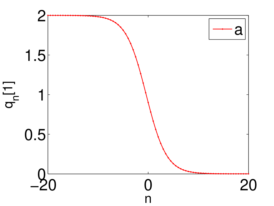
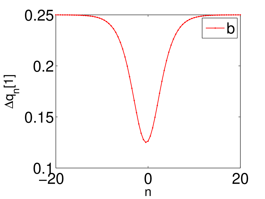
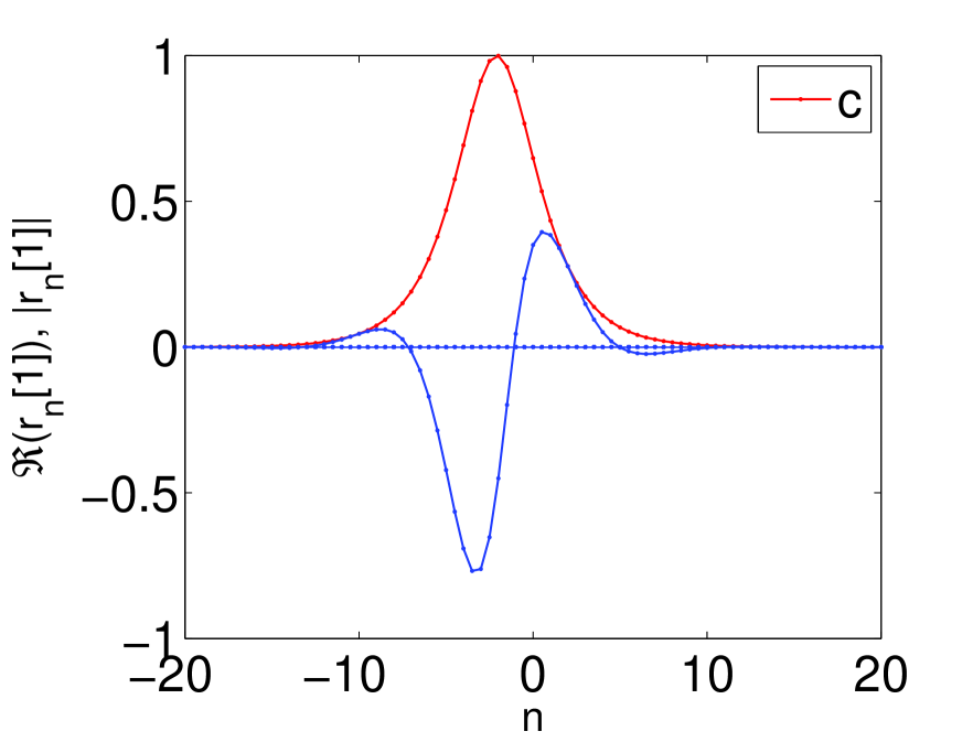
Figure 1: One-(kink and dark) soliton solutions in figures (a and b) respectively, with the choice of parameters $t=0.1,\;\varrho=0.25,\;\lambda_{1}=1+\dot{\imath}$ and in figure (c); red line: $|r_{n}[1]|$, blue line $\Re{(r_{n}[1])}$ with $t=1,\;\varrho=0.5,\;\lambda_{1}=1+\dot{\imath}$.

For two soliton, we take the matrices $\mathcal{E}^{(2)},\;\mathcal{F}_{n,\;1},\;\mathcal{F}_{n,\;2},\;\Lambda_{1}$ and $\Lambda_{2}$ to be

$$\mathcal{E}^{(2)}=\left(\begin{array}[]{cc}0&0\\ 0&0\\ 1&0\\ 0&1\\ \end{array}\right),$$ (4.32)

$$\mathcal{F}_{n,\;1}=\left(\begin{array}[]{cc}f^{(1)}_{n,\;11}&f^{(2)}_{n,\;12}\\ f^{(1)}_{n,\;21}&f^{(2)}_{n,\;22}\end{array}\right),\quad\mathcal{F}_{n,\;2}=\left(\begin{array}[]{cc}f^{(3)}_{n,\;11}&f^{(4)}_{n,\;12}\\ f^{(3)}_{n,\;21}&f^{(4)}_{n,\;22}\end{array}\right),$$ (4.37)

$$\Lambda_{1}=\left(\begin{array}[]{cc}\lambda_{1}&0\\ 0&{\lambda}_{2}\\ \end{array}\right),\quad\qquad\Lambda_{2}=\left(\begin{array}[]{cc}\lambda_{3}&0\\ 0&{\lambda}_{4}\\ \end{array}\right),$$ (4.42)

so that the matrices $\mathcal{F}_{n}$ and $\widehat{\mathcal{F}}_{n}$ become

$$\mathcal{F}_{n} = \left(\begin{array}[]{cc}\mathcal{F}_{n,\;1}&\mathcal{F}_{n,\;2}\\ \mathcal{F}_{n,\;1}\Lambda_{1}&\mathcal{F}_{n,\;2}\Lambda_{2}\end{array}\right)=\left(\begin{array}[]{c:c}\begin{array}[]{cc}f^{(1)}_{n,\;11}&f^{(2)}_{n,\;12}\\ f^{(1)}_{n,\;21}&f^{(2)}_{n,\;22}\end{array}&\begin{array}[]{cc}f^{(3)}_{n,\;11}&f^{(4)}_{n,\;12}\\ f^{(3)}_{n,\;21}&f^{(4)}_{n,\;22}\end{array}\\ \hdashline\begin{array}[]{cc}\lambda_{1}f^{(1)}_{n,\;11}&\lambda_{2}f^{(2)}_{n,\;12}\\ \lambda_{1}f^{(1)}_{n,\;21}&\lambda_{2}f^{(2)}_{n,\;22}\\ \end{array}&\begin{array}[]{cc}\lambda_{3}f^{(3)}_{n,\;11}&\lambda_{4}f^{(4)}_{n,\;12}\\ \lambda_{3}f^{(3)}_{n,\;21}&\lambda_{4}f^{(4)}_{n,\;22}\\ \end{array}\end{array}\right),$$ (4.55)

$$\widehat{\mathcal{F}}_{n} = \left(\begin{array}[]{cc}\mathcal{F}_{n,\;1}\Lambda_{1}^{2}&\mathcal{F}_{n,\;2}\Lambda_{2}^{2}\end{array}\right)=\left(\begin{array}[]{c:c}\begin{array}[]{cc}\lambda_{1}^{2}f^{(1)}_{n,\;11}&\lambda_{2}^{2}f^{(2)}_{n,\;12}\\ \lambda_{1}^{2}f^{(1)}_{n,\;21}&\lambda_{2}^{2}f^{(2)}_{n,\;22}\\ \end{array}&\begin{array}[]{cc}\lambda_{3}^{2}f^{(3)}_{n,\;11}&\lambda_{4}^{2}f^{(4)}_{n,\;12}\\ \lambda_{3}^{2}f^{(3)}_{n,\;21}&\lambda_{4}^{2}f^{(4)}_{n,\;22}\\ \end{array}\end{array}\right).$$ (4.62)

The two-fold DT on the scalar fields $q_{n}$ and $r_{n}$ is given by

$$q_{n}^{[2]} = q_{n}+\dot{\imath}\Theta^{(2)}_{n,\;11},$$ (4.63)

$$r_{n}^{[2]} = \dot{\imath}\Theta^{(2)}_{n,\;12},$$ (4.64)

where the matrix elements $\Theta^{(2)}_{n,\;11},\;\Theta^{(2)}_{n,\;12}$ can be computed as ratios of determinants

$$\Theta_{n,\;11}^{(2)} = \left|\begin{array}[]{cc}\mathcal{F}_{n}&\mathcal{E}^{(2)}_{1}\\ (\widehat{\mathcal{F}}_{n})_{1}&\framebox{$O$}\end{array}\right|=\left|\begin{array}[]{ccccc}f^{(1)}_{n,\;11}&f^{(2)}_{n,\;12}&f^{(3)}_{n,\;11}&f^{(4)}_{n,\;12}&0\\ f^{(1)}_{n,\;21}&f^{(2)}_{n,\;22}&f^{(3)}_{n,\;21}&f^{(4)}_{n,\;22}&0\\ \lambda_{1}f^{(1)}_{n,\;11}&\lambda_{2}f^{(2)}_{n,\;12}&\lambda_{3}f^{(3)}_{n,\;11}&\lambda_{4}f^{(4)}_{n,\;12}&1\\ \lambda_{1}f^{(1)}_{n,\;21}&\lambda_{2}f^{(2)}_{n,\;22}&\lambda_{3}f^{(3)}_{n,\;21}&\lambda_{4}f^{(4)}_{n,\;22}&0\\ \lambda_{1}^{2}f^{(1)}_{n,\;11}&\lambda_{2}^{2}f^{(2)}_{n,\;12}&\lambda_{3}^{2}f^{(3)}_{n,\;11}&\lambda_{4}^{2}f^{(4)}_{n,\;12}&\framebox{$0$}\end{array}\right|,$$ (4.72)

$$= -\frac{\det\left(\begin{array}[]{cccc}f^{(1)}_{n,\;11}&f^{(2)}_{n,\;12}&f^{(3)}_{n,\;11}&f^{(4)}_{n,\;12}\\ f^{(1)}_{n,\;21}&f^{(2)}_{n,\;22}&f^{(3)}_{n,\;21}&f^{(4)}_{n,\;22}\\ \lambda_{1}^{2}f^{(1)}_{n,\;11}&\lambda_{2}^{2}f^{(2)}_{n,\;12}&\lambda_{3}^{2}f^{(3)}_{n,\;11}&\lambda_{4}^{2}f^{(4)}_{n,\;12}\\ \lambda_{1}f^{(1)}_{n,\;21}&\lambda_{2}f^{(2)}_{n,\;22}&\lambda_{3}f^{(3)}_{n,\;21}&\lambda_{4}f^{(4)}_{n,\;22}\end{array}\right)}{\det\left(\begin{array}[]{cccc}f^{(1)}_{n,\;11}&f^{(2)}_{n,\;12}&f^{(3)}_{n,\;11}&f^{(4)}_{n,\;12}\\ f^{(1)}_{n,\;21}&f^{(2)}_{n,\;22}&f^{(3)}_{n,\;21}&f^{(4)}_{n,\;22}\\ \lambda_{1}f^{(1)}_{n,\;11}&\lambda_{2}f^{(2)}_{n,\;12}&\lambda_{3}f^{(3)}_{n,\;11}&\lambda_{4}f^{(4)}_{n,\;12}\\ \lambda_{1}f^{(1)}_{n,\;21}&\lambda_{2}f^{(2)}_{n,\;22}&\lambda_{3}f^{(3)}_{n,\;21}&\lambda_{4}f^{(4)}_{n,\;22}\end{array}\right)}.$$ (4.81)

Similarly, the matrix elements $\Theta_{n,\;12}^{(2)}$ are

$$\Theta_{n,\;12}^{(2)} = -\frac{\det\left(\begin{array}[]{cccc}f^{(1)}_{n,\;11}&f^{(2)}_{n,\;12}&f^{(3)}_{n,\;11}&f^{(4)}_{n,\;12}\\ f^{(1)}_{n,\;21}&f^{(2)}_{n,\;22}&f^{(3)}_{n,\;21}&f^{(4)}_{n,\;22}\\ \lambda_{1}f^{(1)}_{n,\;11}&\lambda_{2}f^{(2)}_{n,\;12}&\lambda_{3}f^{(3)}_{n,\;11}&\lambda_{4}f^{(4)}_{n,\;12}\\ \lambda_{1}^{2}f^{(1)}_{n,\;11}&\lambda_{2}^{2}f^{(2)}_{n,\;12}&\lambda_{3}^{2}f^{(3)}_{n,\;11}&\lambda_{4}^{2}f^{(4)}_{n,\;12}\end{array}\right)}{\det\left(\begin{array}[]{cccc}f^{(1)}_{n,\;11}&f^{(2)}_{n,\;12}&f^{(3)}_{n,\;11}&f^{(4)}_{n,\;12}\\ f^{(1)}_{n,\;21}&f^{(2)}_{n,\;22}&f^{(3)}_{n,\;21}&f^{(4)}_{n,\;22}\\ \lambda_{1}f^{(1)}_{n,\;11}&\lambda_{2}f^{(2)}_{n,\;12}&\lambda_{3}f^{(3)}_{n,\;11}&\lambda_{4}f^{(4)}_{n,\;12}\\ \lambda_{1}f^{(1)}_{n,\;21}&\lambda_{2}f^{(2)}_{n,\;22}&\lambda_{3}f^{(3)}_{n,\;21}&\lambda_{4}f^{(4)}_{n,\;22}\end{array}\right)}.$$ (4.90)

By substituting equations (4.72)-(4.90) into equations (4.63)-(4.64) respectively, we get the two-fold DT on the fields $q_{n}$ and $r_{n}$. Further, we use $f^{(2l)}_{n,\;22}=(-1)^{2l}\bar{f}^{(2l-1)}_{n,\;11},\;f^{(2l)}_{n,\;12}=(-1)^{2l-1}\bar{f}^{(2l-1)}_{n,\;21}$ and $\lambda_{2l}=\bar{\lambda}_{2l-1}$ where $l=1,\;2$ in equations (4.63) and (4.64) to obtain two-soliton solutions of the complex sdCD system. These solutions are plotted in figure 2

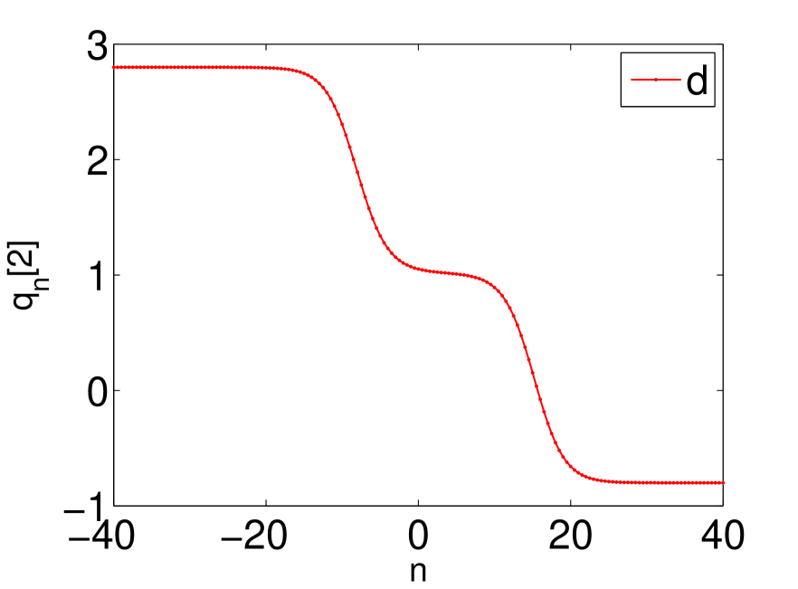
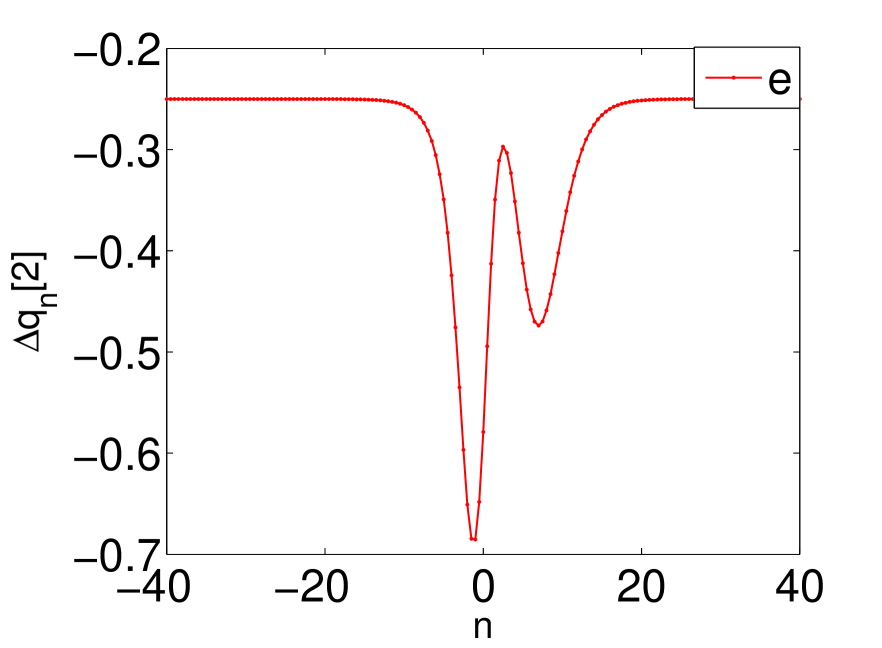
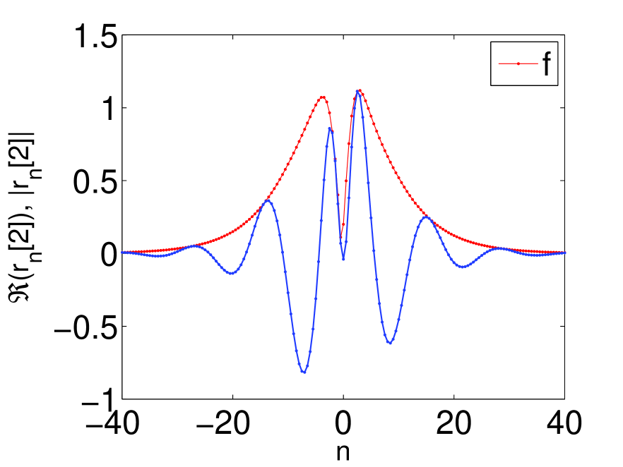
Figure 2: Two-(kink and dark) soliton solutions in figures (d and e) respectively, with the choice of parameters $t=1,\;\varrho=-0.25,\;\lambda_{1}=0.1+0.8\dot{\imath},\;\lambda_{2}=1-\dot{\imath}$ and in figure (f); red line: $|r_{n}[2]|$, blue line $\Re{(r_{n}[2])}$ with $t=0.1,\;\varrho=0.8,\;\lambda_{1}=1+\dot{\imath},\;\lambda_{2}=3-\dot{\imath}$.

To get three-soliton solution, we take three particular matrix solutions $\mathcal{F}_{n,\;k}$ with the eigenvalue matrices $\Lambda_{k}$ ($k=1,\;2,\;3$). With these particular solutions, we obtain three soliton solutions depicted in figure 3

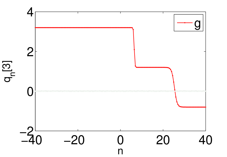
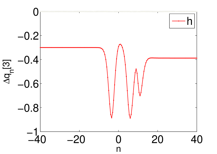
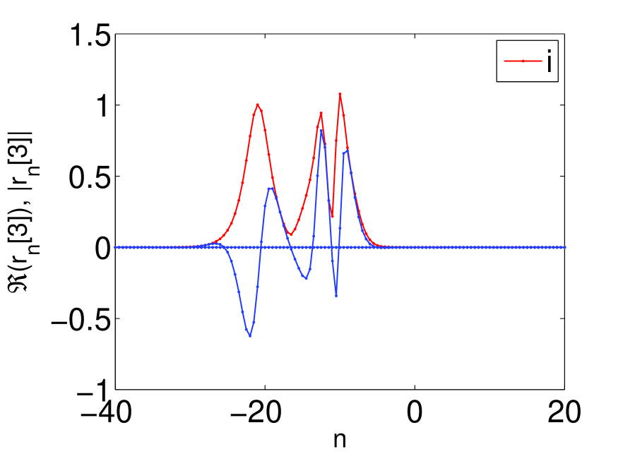
Figure 3: Three-kink solution in figure (g) with $t=20,\;\varrho=-1,\;\lambda_{1}=3+\dot{\imath},\;\lambda_{2}=1+\dot{\imath},\;\lambda_{3}=-0.1-\dot{\imath}$, dark soliton in (h) with $t=2,\;\varrho=-0.3,\;\lambda_{1}=0.3+\dot{\imath},\;\lambda_{2}=0.1-\dot{\imath},\;\lambda_{3}=-1-\dot{\imath}$ and in figure (i); red line: $|r_{n}[3]|$, blue line $\Re{(r_{n}[3])}$ with $t=12,\;\varrho=0.6,\;\lambda_{1}=0.8-\dot{\imath},\;\lambda_{2}=0.5+\dot{\imath},\;\lambda_{3}=-0.5-\dot{\imath}$.

Now, we would like to reduce the semi-discrete solutions of complex sdCD system to those of continuous solutions of the complex CD system by applying continuum limit. For this, replace $\varrho\rightarrow\delta\varrho$ and send $\delta$ to zero, then equations (4.25)-(4.26) respectively reduce to the form

$$q^{[1]} = q-\dot{\imath}\left(\lambda_{1R}+\dot{\imath}\lambda_{1I}\tanh a\right),$$ (4.91)

$$r^{[1]} = \lambda_{1I}e^{\dot{\imath}b}\textrm{sech}a,$$ (4.92)

where

$$a=-\lambda_{1I}\left(\frac{2\varrho}{\left|\lambda_{1}\right|^{2}}x+t\right),\qquad b=-\lambda_{1R}\left(\frac{2\varrho}{\left|\lambda_{1}\right|^{2}}x-t\right).$$ (4.93)

Equations (4.91)-(4.92) represents one-soliton solution of the complex CD system (2.79)-(2.80). Similarly, one can also find the two- and three soliton solutions of the complex CD system (2.79)-(2.80) by applying continuum the limit on the solutions as obtained for the complex sdCD system.

4.2 2-component complex sdCD system

For 2-component complex sdCD system, the $4\times 4$ matrix $\mathcal{U}_{n}$ takes the form

$$\mathcal{U}_{n}=-\dot{\imath}\left(\begin{array}[]{cccc}q_{n}&0&r_{n}^{(1)}&r_{n}^{(2)}\\ 0&q_{n}&-\bar{r}_{n}^{(2)}&\bar{r}_{n}^{(1)}\\ \bar{r}_{n}^{(1)}&-r_{n}^{(2)}&-q_{n}&0\\ \bar{r}_{n}^{(2)}&r_{n}^{(1)}&0&-q_{n}\end{array}\right).$$ (4.94)

The matrix $\Theta_{n}^{(K)}$ in equation (3.33) becomes

$$\Theta_{n}^{(K)}=\left(\begin{array}[]{c:c}\begin{array}[]{cc}\Theta^{(K)}_{n,\;11}&\Theta^{(K)}_{n,\;12}\\ \Theta^{(K)}_{n,\;21}&\Theta^{(K)}_{n,\;22}\end{array}&\begin{array}[]{cc}\Theta^{(K)}_{n,\;13}&\Theta^{(K)}_{n,\;14}\\ \Theta^{(K)}_{n,\;23}&f^{(K)}_{n,\;24}\end{array}\\ \hdashline\begin{array}[]{cc}\Theta^{(K)}_{n,\;31}&\Theta^{(K)}_{n,\;32}\\ \Theta^{(K)}_{n,\;41}&\Theta^{(K)}_{n,\;42}\end{array}&\begin{array}[]{cc}\Theta^{(K)}_{n,\;33}&\Theta^{(K)}_{n,\;34}\\ \Theta^{(K)}_{n,\;43}&f^{(K)}_{n,\;44}\end{array}\end{array}\right)=\left|\begin{array}[]{cc}\mathcal{F}_{n}&\mathcal{E}^{(K)}\\ \mathcal{\widehat{F}}_{n}&\framebox{$O$}\end{array}\right|.$$ (4.95)

In this case, $\mathcal{E}^{(K)}$ are $4K\times 4$ and $\mathcal{\widehat{F}}_{n},\;\mathcal{F}_{n}$ are the $4\times 4K,\;4K\times 4K$ matrices respectively. From equations (3.32) and (4.94)-(4.95), the $K$-fold DT on the solutions of the 2-component complex sdCD system is given by

$$q_{n}^{[K]} = q_{n}+\dot{\imath}\Theta_{n,\;11}^{(K)},$$ (4.96)

$$r_{n}^{(1)[K]} = \dot{\imath}\Theta_{n,\;13}^{(K)},$$ (4.97)

$$r_{n}^{(2)[K]} = \dot{\imath}\Theta_{n,\;14}^{(K)},$$ (4.98)

The matrix valued solution $\Psi_{n}$ to the Lax pair of the 2-component sdCD system is written as

$$\Psi_{n}=\left(\begin{array}[]{c:c}\left(1-\dot{\imath}\varrho\lambda^{-1}\right)^{n}e^{\frac{\dot{\imath}\lambda}{2}t}I_{2\times 2}&O\\ \hdashline O&\left(1+\dot{\imath}\varrho\lambda^{-1}\right)^{n}e^{-\frac{\dot{\imath}\lambda}{2}t}I_{2\times 2}\end{array}\right)$$ (4.99)

To construct matrix $\mathcal{F}_{n}$ from a matrix solution $\Psi_{n}$, let us take columns i.e.,

$$\left|e_{1}\right\rangle = \left(\begin{array}[]{c}\epsilon_{1}\\ \epsilon_{2}\\ -1\\ 0\end{array}\right),\quad\left|e_{2}\right\rangle=\left(\begin{array}[]{c}\bar{\epsilon}_{2}\\ -\bar{\epsilon}_{1}\\ 0\\ 1\end{array}\right),$$ (4.108)

$$\left|e_{3}\right\rangle = \left(\begin{array}[]{c}1\\ 0\\ \bar{\epsilon}_{1}\\ -\epsilon_{2}\end{array}\right),\quad\left|e_{4}\right\rangle=\left(\begin{array}[]{c}0\\ 1\\ \bar{\epsilon}_{2}\\ \epsilon_{1}\end{array}\right),$$ (4.117)

where $\epsilon_{1},\;\epsilon_{2}$ are complex constants. For $\Lambda_{k}=\text{diag}(\lambda_{k},\;\lambda_{k},\;\bar{\lambda}_{k},\;\bar{\lambda}_{k}),\;k=1,\;2,\;...,\;K$, we have different particular matrix solutions as

$$\mathcal{F}_{n,\;k} = \left(\Psi_{n}\left|e_{1}\right\rangle,\;\Psi_{n}\left|e_{2}\right\rangle,\;\Psi_{n}\left|e_{3}\right\rangle,\;\Psi_{n}\left|e_{4}\right\rangle\right),$$ (4.122)

$$= \left(\begin{array}[]{cccc}\epsilon_{1}x(\lambda_{k})&\bar{\epsilon}_{2}x(\lambda_{k})&x(\bar{\lambda}_{k})&0\\ \epsilon_{2}x(\lambda_{k})&-\bar{\epsilon}_{1}x(\lambda_{k})&0&x(\bar{\lambda}_{k})\\ -\bar{x}(\lambda_{k})&0&\bar{\epsilon}_{1}\bar{x}(\bar{\lambda}_{k})&\bar{\epsilon}_{2}\bar{x}(\bar{\lambda}_{k})\\ 0&\bar{x}(\lambda_{k})&-\epsilon_{2}\bar{x}(\bar{\lambda}_{k})&\epsilon_{1}\bar{x}(\bar{\lambda}_{k})\end{array}\right),$$

where $x(\lambda_{k})=\left(1-\dot{\imath}\varrho\lambda^{-1}_{k}\right)^{n}e^{\frac{\dot{\imath}\lambda_{k}}{2}t}$ and $\bar{x}(\lambda_{k})=\left(1+\dot{\imath}\varrho\lambda^{-1}_{k}\right)^{n}e^{-\frac{\dot{\imath}\lambda_{k}}{2}t}$. To calculate soliton solutions explicitly of the 2-component sdCD system, we proceed as follows. For one soliton $K=1$, the matrices $\mathcal{E}^{(1)},\;\Lambda_{1},\;\mathcal{F}_{n},\;\widehat{\mathcal{F}}_{n}$ are given by

$$\mathcal{E}^{(1)}=I_{4}=\left(\begin{array}[]{cccc}1&0&0&0\\ 0&1&0&0\\ 0&0&1&0\\ 0&0&0&1\end{array}\right),$$ (4.127)

$$\mathcal{F}_{n}=\mathcal{F}_{n,\;1}=\left(\begin{array}[]{cccc}\epsilon_{1}x(\lambda_{1})&\bar{\epsilon}_{2}x(\lambda_{1})&x(\bar{\lambda}_{1})&0\\ \epsilon_{2}x(\lambda_{1})&-\bar{\epsilon}_{1}x(\lambda_{1})&0&x(\bar{\lambda}_{1})\\ -\bar{x}(\lambda_{1})&0&\bar{\epsilon}_{1}\bar{x}(\bar{\lambda}_{1})&\bar{\epsilon}_{2}\bar{x}(\bar{\lambda}_{1})\\ 0&\bar{x}(\lambda_{1})&-\epsilon_{2}\bar{x}(\bar{\lambda}_{1})&\epsilon_{1}\bar{x}(\bar{\lambda}_{1})\end{array}\right),\Lambda_{1}=\left(\begin{array}[]{cccc}\lambda_{1}&0&0&0\\ 0&\lambda_{1}&0&0\\ 0&0&\bar{\lambda}_{1}&0\\ 0&0&0&\bar{\lambda}_{1}\end{array}\right),$$ (4.136)

$$\widehat{\mathcal{F}}_{n}=\mathcal{F}_{n,\;1}\Lambda_{1}=\left(\begin{array}[]{cccc}\epsilon_{1}\lambda_{1}x(\lambda_{1})&\bar{\epsilon}_{2}\lambda_{1}x(\lambda_{1})&\bar{\lambda}_{1}x(\bar{\lambda}_{1})&0\\ \epsilon_{2}\lambda_{1}x(\lambda_{1})&-\bar{\epsilon}_{1}{\lambda}_{1}x(\lambda_{1})&0&\bar{\lambda}_{1}x(\bar{\lambda}_{1})\\ -\lambda_{1}\bar{x}(\lambda_{1})&0&\bar{\epsilon}_{1}\bar{\lambda}_{1}\bar{x}(\bar{\lambda}_{1})&\bar{\epsilon}_{2}\bar{\lambda}_{1}\bar{x}(\bar{\lambda}_{1})\\ 0&\lambda_{1}\bar{x}(\lambda_{1})&-\epsilon_{2}\bar{\lambda}_{1}\bar{x}(\bar{\lambda}_{1})&\epsilon_{1}\bar{\lambda}_{1}\bar{x}(\bar{\lambda}_{1})\end{array}\right).$$ (4.141)

By substituting (4.127) in (4.96), the one-fold DT $q_{n}[1]$ can be calculated as

$${q}_{n}[1] = q_{n}+(\Theta_{n}^{[1]})_{11}=q_{n}+\left|\begin{array}[]{cc}\mathcal{F}_{n,\;1}&\mathcal{E}^{(1)}_{1}\\ (\mathcal{\widehat{F}}_{n,\;1})_{1}&\framebox{$0$}\end{array}\right|,$$ (4.144)

$$= q_{n}+\left|\begin{array}[]{ccccc}\epsilon_{1}x(\lambda_{1})&\bar{\epsilon}_{2}x(\lambda_{1})&x(\bar{\lambda}_{1})&0&1\\ \epsilon_{2}x(\lambda_{1})&-\bar{\epsilon}_{1}x(\lambda_{1})&0&x(\bar{\lambda}_{1})&0\\ -\bar{x}(\lambda_{1})&0&\bar{\epsilon}_{1}\bar{x}(\bar{\lambda}_{1})&\bar{\epsilon}_{2}\bar{x}(\bar{\lambda}_{1})&0\\ 0&\bar{x}(\lambda_{1})&-\epsilon_{2}\bar{x}(\bar{\lambda}_{1})&\epsilon_{1}\bar{1}(\bar{\lambda}_{1})&0\\ \epsilon_{1}\lambda_{1}x(\lambda_{1})&\bar{\epsilon}_{2}\lambda_{1}x(\lambda_{1})&\bar{\lambda}_{1}x(\bar{\lambda}_{1})&0&\framebox{$0$}\end{array}\right|,$$ (4.150)

$$= q_{n}-\frac{\det\left(\begin{array}[]{cccc}\epsilon_{1}\lambda_{1}x(\lambda_{1})&\bar{\epsilon}_{2}\lambda_{1}x(\lambda_{1})&\bar{\lambda}_{1}x(\bar{\lambda}_{1})&0\\ \epsilon_{2}x(\lambda_{1})&-\bar{\epsilon}_{1}x(\lambda_{1})&0&x(\bar{\lambda}_{1})\\ -\bar{x}(\lambda_{1})&0&\bar{\epsilon}_{1}\bar{x}(\bar{\lambda}_{1})&\bar{\epsilon}_{2}\bar{x}(\bar{\lambda}_{1})\\ 0&\bar{x}(\lambda_{1})&-\epsilon_{2}\bar{x}(\bar{\lambda}_{1})&\epsilon_{1}\bar{x}(\bar{\lambda}_{1})\end{array}\right)}{\det\left(\begin{array}[]{cccc}\epsilon_{1}x(\lambda_{1})&\bar{\epsilon}_{2}x(\lambda_{1})&x(\bar{\lambda}_{1})&0\\ \epsilon_{2}x(\lambda_{1})&-\bar{\epsilon}_{1}x(\lambda_{1})&0&x(\bar{\lambda}_{1})\\ -\bar{x}(\lambda_{1})&0&\bar{\epsilon}_{1}\bar{x}(\bar{\lambda}_{1})&\bar{\epsilon}_{2}\bar{x}(\bar{\lambda}_{1})\\ 0&\bar{x}(\lambda_{1})&-\epsilon_{2}\bar{x}(\bar{\lambda}_{1})&\epsilon_{1}\bar{1}(\bar{\lambda}_{1})\end{array}\right)}.$$ (4.159)

Simplifying the above expression, we get

$${q}_{n}[1] = q_{n}-\dot{\imath}\frac{\lambda_{1}\left(|\epsilon_{1}|^{2}+|\epsilon_{2}|^{2}\right)\chi_{n}^{+}+\bar{\lambda}_{1}\chi_{n}^{-}}{\left(|\epsilon_{1}|^{2}+|\epsilon_{2}|^{2}\right)\chi_{n}^{+}+\chi_{n}^{-}}.$$ (4.160)

Similarly

$${r}_{n}^{(1)}[1] = \dot{\imath}\epsilon_{1}\frac{\left(\bar{\lambda}_{1}-\lambda_{1}\right)\varphi_{n}^{+}}{\left(|\epsilon_{1}|^{2}+|\epsilon_{2}|^{2}\right)\chi_{n}^{+}+\chi_{n}^{-}},$$ (4.161)

$${r}_{n}^{(2)}[1] = \dot{\imath}\bar{\epsilon}_{2}\frac{\left(\bar{\lambda}_{1}-\lambda_{1}\right)\varphi_{n}^{+}}{\left(|\epsilon_{1}|^{2}+|\epsilon_{2}|^{2}\right)\chi_{n}^{+}+\chi_{n}^{-}}.$$ (4.162)

where $\chi_{n}^{+},\;\chi_{n}^{-}$ and $\varphi_{n}^{+}$ are given in (4.27). Equations (4.160)-(4.162) represent one-soliton solution of the 2-component sdCD system (2.49)-(2.50). The plot of equations (4.160)-(4.162) has been sketched out as in the figures 4-5

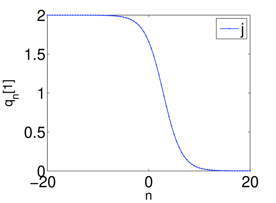
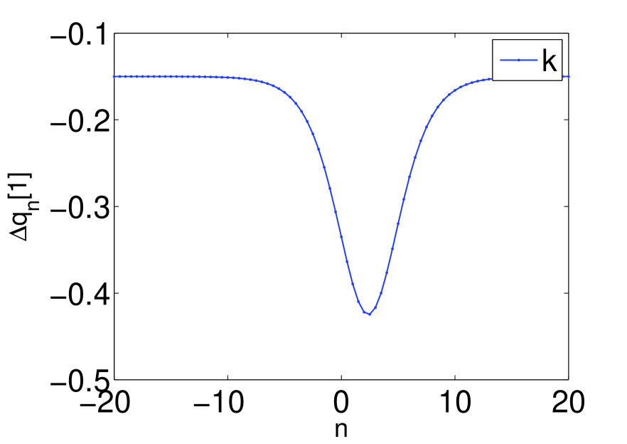
Figure 4: Kink and dark solutions in figures (j and k) with $t=0.1,\;\varrho=0.15,\;\lambda_{1}=0.3-\dot{\imath},\;\epsilon_{1}=1-\dot{\imath},\;\epsilon_{2}=1+\dot{\imath}$.

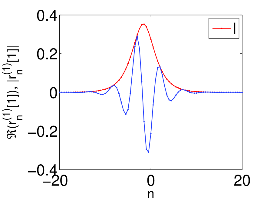
Figure 5: Bright and periodic solutions in figures (l and m); red line: $|r_{n}|$, blue line $\Re{(r_{n})}$ with $t=0.1,\;\varrho=0.8,\;\lambda_{1}=1-0.5\dot{\imath},\;\epsilon_{1}=1-\dot{\imath},\;\epsilon_{2}=1+\dot{\imath}$.

And the solutions obtained in equations (4.160)-(4.162) in the continuum limit can be written as

$$q^{[1]} = q-\dot{\imath}\left(\lambda_{1R}+\dot{\imath}\tanh\left(a+\ln\sqrt{\epsilon}\right)\right),$$ (4.163)

$$r^{(1)[1]} = \frac{\epsilon_{1}\lambda_{1I}e^{\dot{\imath}b}}{\sqrt{\epsilon}}\textrm{sech}\left(a+\ln\sqrt{\epsilon}\right),\quad r^{(2)[1]}=\frac{\bar{\epsilon}_{2}\lambda_{1I}e^{\dot{\imath}b}}{\sqrt{\epsilon}}\textrm{sech}\left(a+\ln\sqrt{\epsilon}\right),$$ (4.164)

where $\epsilon=|\epsilon_{1}|^{2}+|\epsilon_{2}|^{2}$. Equations (4.163)-(4.164) represents one-soliton solutions of the 2-component complex CD system.

5 Concluding remarks

In this paper, we have studied integrable discretization of complex and multi-component coupled dispersionless system. By writing down the Lax pair of the systems, we have computed one-, two- and three-soliton solutions of complex and 2-component complex coupled dispersionless system. We have also shown that, the solutions obtained for the complex and 2-component complex sdCD system reduced to the solutions of the respective continuous complex and 2-component complex CD system by applying continuum limit. The study can be further extended by investigating multicomponent and matrix generalizations of related integrable systems. An important example of such systems is the short pulse equation. We shall address these research problems in forthcoming work.

References

- [1] L. D. Faddeev, L. A. Takhtajan, Hamiltonian Methods in the Theory of Solitons (Springer-Verlag, Berlin, 1987).
- [2] M. J. Ablowitz, B. Prinari, A. D. Trubatch, Discrete and Continuous Nonlinear Schrödinger Systems. Cambridge University Press, Cambridge, 2004.
- [3] Y. B. Suris, The Problem of Integrable Discretization: Hamiltonian Approach. Basel, Birhauser, 2003.
- [4] B. Grammaticos, T. Tamizhmani, and Y. Kosmann-Schwarzbach, Discrete integrable systems, Lecture notes in Physics, 644, Springer-Verlag, Berlin, 2004.
- [5] D. Levi, P. Olver , Z. Thomova, and P. Winternitz, Symmetries and Integrability of Difference Equations, London Mathematical Society Lecture Notes series: 381, Cambridge University Press, 2011.
- [6] A. I. Bobenko and Y. B. Suris, Discrete Differential Geometry: Integrable Structure, Graduate Studies in Mathematics Volume 98, AMS, 2008.
- [7] H. W. A. Riaz, M. Hassan, On soliton solutions of multi-component semi-discrete short pulse equation, J. Phys. Commun. 2 (2018) 025005.
- [8] K. Takasaki, T. Takebe, Quasi-classical limit of Toda hierarchy and Winfinity symmetries, Lett. Math. Phys. 28 (1993) 165.
- [9] K. Takasaki, T. Takebe, Integrable hierarchies and dispersionless limit, Rev. Math. Phys. 7 (1995) 743.
- [10] K. Takasaki, Dispersionless Toda hierarchy and two-dimensional string theory, Commun. Math. Phys. 170 (1995) 743.
- [11] K. Takasaki, Dispersionless Toda hierarchy and two-dimensional string theory, Commun. Math. Phys. 170 (1995) 743.
- [12] M. Dunajski, Interpolating Dispersionless Integrable System, J. Phys. A 41, 315202 (2008) doi:10.1088/1751-8113/41/31/315202 [arXiv:0804.1234 [nlin.SI]].
- [13] E. V. Ferapontov and B. Kruglikov, Dispersionless integrable systems in 3D and Einstein-Weyl geometry, J. Diff. Geom. 97, no. 2, 215 (2014) [arXiv:1208.2728 [math-ph]].
- [14] B. Kruglikov and O. Morozov, Integrable dispersionless PDEs in 4D, their symmetry pseudogroups and deformations, Lett. Math. Phys. 105, no. 12, 1703 (2015). doi:10.1007/s11005-015-0800-z
- [15] K. Konno, H. Oono, New coupled integrable dispersionless equations, J. Phys. Soc. Jpn. 63 (1994) 477.
- [16] H. Kakuhata, K. Konno, A generalization of coupled integrable, dispersionless system, J. Phys. Soc. Jpn. 65, (1996) 340.
- [17] K. Konno, Integrable coupled dispersionless equations, Appl. Anal. 57 (1995) 209.
- [18] R. Hirota, S. Tsujimoto, Note on “New coupled integrable dispersionless equations”, J. Phys. Soc. Jpn. 63 (1994) 3533.
- [19] V. P. Kotlyarov, On equations gauge equivalent to the sine-Gordon and Pohlmeyer-Lund-Regge equations, J. Phys. Soc. Jpn. 63, (1994) 3535.
- [20] S. F. Shen, B. F. Feng, Y. Ohta, From the real and complex coupled dispersionless equations to the real and complex short pulse equations, Stud. Appl. Math 136 (2016) 64.
- [21] T. Alagesan, Y. Chung, K. Nakkeeran, Backlund transformation and soliton solutions for the coupled dispersionless equations, Chaos Solitons Fractals 21 (2004) 63.
- [22] M. Hassan, Darboux transformation of the generalized coupled dispersionless integrable system, J. Phys. A: Math. Theor. 42 (2009) 65203.
- [23] N. Mushahid, M. Hassan, A noncommutative coupled dispersionless system, Darboux transformation and explicit solutions, Mod. Phys. Lett. A 29 (2014) 1450206.
- [24] S. Y. Lou, G. F. Yu, A generalization of the coupled integrable dispersionless equations, Math. Meth. Appl. Sci. 39 (2016) 4025.
- [25] L. Vinet, G. F. Yu, Discrete analogues of the generalized coupled integrable dispersionless equations, J. Phys. A: Math. Theor. 46 (2013) 175205.
- [26] L. Vinet, G. F. Yu, On the discretization of the coupled integrable dispersionless equations , J. Nolinear. Math. Phys. 20 (2013) 106.
- [27] H. W. A. Riaz, M. Hassan, Darboux transformation of a semi-discrete coupled dispersionless integrable system, Commun. Nonlinear Sci. Numer. Simulat. 48 (2017) 387.
- [28] H. W. A. Riaz, M. Hassan, A discrete generalized coupled dispersionless integrable system and its multisoliton solutions, J. Math. Anal. Appl. 458 (2018) 1639.
- [29] H. W. A. Riaz, M. Hassan, Multi-component semi-discrete coupled dispersionless integrable system, its lax pair and Darboux transformation, Commun. Nonlinear Sci. Numer. Simulat. 61 (2018) 71.
- [30] Z. W. Xu, G. F. Yu, Z. N. Zhu, Soliton dynamics to the multi-component complex coupled integrable dispersionless equation, Commun. Nonlinear Sci. Numer. Simulat. 40 (2016) 28.
- [31] BF Feng, K. Maruno and Y. Ohta, Integrable semi discretization of a multi-component short pulse equation. J. Math. Phys. 56 (2015) 043502.
- [32] V. B. Matveev, M. A. Salle, Darboux Transformations and Solitons (Berlin: Springer, 1991).
- [33] C. Rogers, W. K. Schief, B cklund and Darboux transformations: geometry and modern applications in soliton theory, Cambridge Texts in Applied Mathematics, Cambridge University Press, Cambridge, 2002.
- [34] C. Gu, H. Hu and Z. Zhou, Darboux Transformations in Integrable Systems, Theory and their Applications to Geometry (Berlin: Springer, 2005).
- [35] H. W. A. Riaz, M. Hassan, Darboux transformation for a semidiscrete short-pulse equation, Theor. Math. Phys. 194 (2018) 360.
- [36] H. W. A. Riaz, M. Hassan, Generalized lattice Heisenberg magnet model and its quasideterminant soliton solutions, Theor. Math. Phys. 195 (2018) 665.
- [37] H. W. A. Riaz, M. Hassan, On soliton solutions of multi-component semi-discrete short pulse equation, J. Phys. Commun. 2 (2018) 025005.
- [38] I. Gelfand, V. Retakh, Determinants of matrices over noncommutative rings, Funct. Anal. Appl. 25 (1991) no. 2, 91-102.