The CARMENES search for exoplanets around M dwarfs

We use spectra from CARMENES, the Calar Alto high-Resolution search for M dwarfs with Exo-earths with Near-infrared and optical Echelle Spectrographs, to search for periods in chromospheric indices in 16 M0 to M2 dwarfs. We measure spectral indices in the H$\alpha$, the Ca ii infrared triplet (IRT), and the Na i D lines to study which of these indices are best-suited to find rotation periods in these stars. Moreover, we test a number of different period-search algorithms, namely the string length method, the phase dispersion minimisation, the generalized Lomb-Scargle periodogram, and the Gaussian process regression with quasi-periodic kernel. We find periods in four stars using H$\alpha$ and in five stars using the Ca ii IRT, two of which have not been found before. Our results show that both H$\alpha$ and the Ca ii IRT lines are well suited for period searches, with the Ca ii IRT index performing slightly better than H$\alpha$. Unfortunately, the Na i D lines are strongly affected by telluric airglow, and we could not find any rotation period using this index. Further, different definitions of the line indices have no major impact on the results. Comparing the different search methods, the string length method and the phase dispersion minimisation perform worst, while Gaussian process models produce the smallest numbers of false positives and non-detections.

1 Introduction

Magnetic activity in late-type dwarfs manifests itself in a plethora of observed phenomena originating in different stellar atmospheric layers. Some of these different activity indicators are coupled to the rotational variability of the star and can therefore be used to measure stellar rotation periods. Knowledge of the rotation period of a given star is crucial for an understanding of its magnetic activity, but also in the context of searches for exoplanets, since inhomogeneities such as spots in the photosphere or plages in the chromosphere in combination with stellar rotation can easily mimic a feigned planetary signal (see e.g. Hatzes, 2013).

The rotation period of a star can be measured using photometric data, using spots on its surface which cause cyclic variability of the light curve of the star while rotating with the star; for field M dwarf stars this method has been extensively used, for example by Díez Alonso et al. (2018); Newton et al. (2017); Suárez Mascareño et al. (2016); West et al. (2015); Irwin et al. (2011), and many others. Alternatively, spectral data can be used, such as index or equivalent width (EW) time series of chromospheric lines. Such index time series carry a rotational imprint if the emitting plage regions are not homogeneously distributed on the stellar surface (see e.g. Mittag et al., 2017; Suárez Mascareño et al., 2015). Traditionally, for such spectroscopic studies in solar-like dwarfs the Ca ii H and K doublet lines are used (Noyes et al., 1984). However, for M dwarfs these lines are hard to access since the pseudo-continuum is very low at these wavelengths, and therefore other spectral indices have been tested for correlation with Ca ii H and K or for use as rotation diagnostics. For example, Díaz et al. (2007) find that the Na i D index correlates with H$\alpha$ for the most active stars (Balmer lines in emission). Walkowicz & Hawley (2009) also find correlations between the Ca ii K and H$\alpha$ emissions for active stars, while for inactive or medium active stars (H$\alpha$ in absorption) the relation between the two indicators remains ambiguous. On the other hand, in the framework of cycle studies for M dwarf stars, Gomes da Silva et al. (2011) find a correlation between Ca ii H and K and Na i D also for less-active stars. Moreover, Martin et al. (2017) find a good correlation between Ca ii H and K and the infrared triplet (IRT) of this ion, located at (vacuum) wavelengths of 8500.35, 8544.44, and 8664.52 Å. A recent study by Schöfer et al. (2018), concentrating on M dwarfs using CARMENES (Quirrenbach et al., 2016) data, shows a correlation between H$\alpha$ and He i D₃ as well as the Ca ii IRT.

Besides the use of different spectral lines for the search of rotation periods, a variety of search methods are available; a comparison of 11 different period-search algorithms for photometric data and seven different object classes (e.g. eruptive, pulsating, rotating) was performed by Graham et al. (2013b), who find that the recovery of the signal strongly depends on the quality of the light curve and that especially for lower-quality light curves the signal recovery depends sensitively on the amplitude off the signal. The best-performing algorithm identified by Graham et al. (2013b) was a conditional entropy-based algorithm.

The purpose of this study is to explore the effects of using different spectral lines and search algorithms on finding rotation periods in M dwarfs. We use a large set of CARMENES high-resolution spectra of 16 relatively inactive early M dwarfs and use spectral indices of H$\alpha$, the Ca ii IRT, and Na i D. Moreover, we compare the following period-search algorithm: Generalized Lomb-Scargle (GLS) periodogram, the string length (SL) method, phase dispersion (PD) minimisation, and Gaussian process (GP) regression with quasi-periodic kernel. Our paper is structured as follows: in Sect. 2 we describe the data we have used, the stellar sample is described in Sect. 3, and in Sect. 4 we define the different activity indices. In Sect. 5 we give some details on the search algorithms that we use and present our results. Finally, a discussion and our conclusions are presented in Sects. 6 and 7, respectively.

2 Observations and data reduction

All spectra discussed in this paper were taken with the CARMENES spectrograph (Quirrenbach et al., 2016) at the 3.5-m Calar Alto telescope during guaranteed time observations for the radial-velocity exo-planet survey. The main scientific objective of CARMENES is the search for low-mass planets orbiting M dwarfs in their habitable zone. For that, the CARMENES consortium is conducting a 750-night survey, targeting $\sim$330 M dwarfs (Alonso-Floriano et al., 2015; Reiners et al., 2018). To date, CARMENES has obtained more than 10 000 high-resolution visible and near-infrared (NIR) spectra. The CARMENES spectrograph is a two-channel, fibre-fed spectrograph covering the wavelength range from 0.52 to 0.96 $\mu$m in the visual channel (VIS) and from 0.96 to 1.71 $\mu$m in the NIR channel with spectral resolution of R $\sim$ 94 600 in VIS and R $\sim$ 80 400 in NIR.

The CARMENES spectra were reduced using the CARMENES reduction pipeline and retrieved from the CARMENES data archive (Caballero et al., 2016b; Zechmeister et al., 2017). To simplify measurements we shifted all spectral lines to laboratory wavelength by correcting for barycentric and stellar radial-velocity shifts. Since we are not interested in high-precision radial-velocity measurements in our context, we use the mean radial velocity for each star as given in the Carmencita database (Caballero et al., 2016a) and used the python package helcorr of PyAstronomy to compute the barycentric shift.

We do not correct for telluric lines, which are normally weak in the vicinity of the H$\alpha$ and Ca ii IRT lines. We do however carefully select our reference bands, avoiding regions affected by telluric lines. Since the airglow of Na i D lines can be several times stronger than the stellar contribution and thus poses a serious challenge to analysis, we excluded the contaminated spectra (for more details see Sect. 4). The exposure times for our program stars vary from about 100 s for the brightest stars to a few hundred seconds, but are typically below 500 s.

3 The stellar sample

Our sample selection starts with all 95 dwarfs of spectral types from M0.0 to M2.0 observed by the CARMENES survey, for which we retrieved all available spectra as of 1 Feb 2018. In this study we investigate periodicity and period search algorithms and focus on early M dwarfs. Later M dwarfs show increasingly frequent flaring, which strongly affects the chromospheric emission lines studied here. Moreover, we limit the sample to stars with more than 50 CARMENES observations without flaring according to our criterion (Sect. 4.1). This choice ensures a mean sampling rate of less than or approximately one every 14 days (more than 50 observations in about 700 days). Nevertheless, the irregular sampling allows for additional studies of periods below the formal Nyquist limit. In our initial sample, only six stars have between 40 and 50 observations distributed over $700$ days and the majority of stars have less than 30 observations, which we consider insufficient for the period analysis. Thus, our selection leaves us with a final target sample of 16 stars of which nine have 100 or more observations.

In Table 1 we list the CARMENES identifier and a more common name, together with the number of spectra used for our period analysis. In addition, we provide relevant information retrieved from Carmencita (Caballero et al., 2016a), such as spectral type, rotational velocity, membership to kinematic populations, and, for nine of them, previously derived rotation periods from photometry or spectroscopy.

Notably, neither M2 nor halo stars fulfil our target-selection criteria. All target stars can be attributed to the thick-disc, disc, or young-disc populations. From CARMENES spectra, Reiners et al. (2018) deduced an upper limit of 2.0 km s^-1 to the rotational velocity of 11 stars, and measured $v\sin{i}$ of five M0.0 and M0.5 dwarfs (see also Jeffers et al. (2018)). For these five stars, we compute an estimated (maximum) rotation period $P_{\rm est}$ assuming an inclination of $90^{\circ}$ and using individual radii from Schweitzer et al. (2018), which are all between 0.57 and 0.64 $R_{\odot}$. These correspond well to a radius of 0.62 $R_{\odot}$ by Kaltenegger & Traub (2009), which is applicable to M0.0 V stars.

While most spectral observations are separated by at least one night, some spectra were obtained at shorter cadence on the same night for engineering purposes. The respective number of these additional densely sampled observations is also given in Table 1. Notable cases are GX And, HD 119850, BD+21 652, and Lalande 21185, for which $53$ %, $18$ %, $7.5$ %, and $7.5$ % of the available spectra were obtained in such single-night runs; these cases are discussed in some detail in Sect. 6.4.

Our sample consists of stars with low to modest activity as reflected in the H$\alpha$ line profiles. None of our sample stars show H$\alpha$ lines in true emission. The most active star is V2689 Ori, whose H$\alpha$ line is just below the level where it would go into emission. On the other hand, BD+21 652 exhibits the deepest H$\alpha$ absorption line and is therefore among the stars with the lowest activity of our sample. More details on the activity of our sample stars are provided in the following section.

Table 1: Properties of the sample stars.

Karmn	Name	No.	No.	Sp.	Ref.	Popc	$v\sin{i}$ d	$P_{\rm est}$	$P_{\rm lit}$	Refe
		spec.a	shortb	type	(SpT)		[km s-1]	[d]	[d]	($P_{\rm lit}$)
J00183+440	GX And	190	112	M1.0	AF15a	D	¡2.0	…	…	…
J01026+623	BD+61 195	68	2	M1.5	AF15a	YD	¡2.0	…	19.9$\pm$ 0.4, 18.4$\pm$ 0.7	DA18, SM17
J04290+219	BD+21 652	161	23	M0.5	Gra06	D	3.9 $\pm$1.4	8.3	25.4$\pm$ 0.3	DA18
J04376+528	BD+52 857	78	11	M0.0	Gra03	D	3.4 $\pm$0.6	8.5	…	…
J05314-036	HD 36395	87	7	M1.5	AF15a	D	¡2.0	…	33.8$\pm$ 0.6, 33.61	DA18, KS07
J05365+113	V2689 Ori	50	12	M0.0	Lep13	YD	3.8 $\pm$0.4	7.5	12.3$\pm$ 0.1, 12.02	DA18, Kir12
J09144+526	HD 79211	115	9	M0.0	AF15a	YD	2.3 $\pm$0.4	12.7	…	…
J09561+627	BD+63 869	57	7	M0.0	PMSU	YD	¡2.0	…	…	…
J10122-037	AN Sex	61	6	M1.5	PMSU	YD	¡2.0	…	21.6$\pm$ 0.2,21.56	DA18,Kir12
J11033+359	Lalande 21185	147	21	M1.5	AF15a	TD	¡2.0	…	48.0	No84
J11054+435	BD+44 2051A	100	7	M1.0	AF15a	TD-D	¡2.0	…	…	…
J13299+102	BD+11 2576	64	7	M0.5	PMSU	D	¡2.0	…	28.0$\pm$ 2.9	SM15
J13457+148	HD 119850	223	58	M1.5	PMSU	D	¡2.0	…	52.3$\pm$ 1.7	SM15
J16167+672S	HD 147379	124	4	M0.0	AF15a	YD	2.7 $\pm$0.2	11.6	…	…
J20533+621	HD 199305	133	2	M1.0	Lep13	D	¡2.0	…	…	…
J22565+165	HD 216899	203	14	M1.5	PMSU	TD	¡2.0	…	39.5$\pm$ 0.2, 37.5$\pm$ 0.1	DA18, SM15

AF15a: Alonso-Floriano et al. (2015); DA18: Díez Alonso et al. (2018); Gra03: Gray et al. (2003); Gra06: Gray et al. (2006); Kir12: Kirkpatrick et al. (2012); KS07: Kiraga & Stepien (2007); Lep13: Lépine et al. (2013); No84: Noyes et al. (1984); PMSU: Reid et al. (1995); SM15: Suárez Mascareño et al. (2015); SM17: Suárez Mascareño et al. (2018)
^a Total number of spectra used in the analysis.
^b Number of spectra obtained at short sub-day cadence.
^c All kinematic population designations are measured by Cortés-Contreras (2016): abbreviations: YD: young disc, D: disc, TD: thick disc, TD-D: thin-to-thick transition disc; there are no halo stars in our sample.
^d All rotational velocities are measured by Reiners et al. (2018) and are included in the catalogue of Jeffers et al. (2018).
^e No84 and SM15 determined spectroscopically, all other periods determined photometrically.

4 Indices and time series

To characterise the stellar activity state for each spectrum, we define activity indices following the method of Robertson et al. (2016). In particular, we use the mean flux density in a spectral band centred on the spectral feature (the so-called line band) and divide by the sum of the average flux density in two reference bands

$$I_{\rm line}=w\,\left(1-\frac{2\cdot\overline{F_{\rm line}}}{\overline{F_{\rm ref1}}+\overline{F_{\rm ref2}}}\right)\;.$$ (1)

Here, $w$ is the width of the line band, and $\overline{F_{\rm line}}$, $\overline{F_{\rm ref1}}$, and $\overline{F_{\rm ref2}}$ are the mean flux densities in the line and the two reference bands, respectively. The thus-defined index resembles a pseudo-EW (pEW) with the difference that we use the mean flux densities and not integrals.

To compute statistical errors for $I_{\rm line}$, we use the pipeline-generated errors on the flux density and a Monte Carlo simulation. Specifically, we compute the index 100 000 times for each line and each spectrum using flux density values randomly drawn from the error distribution and, thus, estimate the standard deviation of the respective index. We consider indices for H$\alpha$, Na i, and the Ca ii IRT. The line and reference bands used are provided in Table 2.

Table 2: Properties of the indices’ line and reference bands.

Line	Line band		Reference bands
	central	full	blue	red
	wavel.	width
	[Å]	[Å]	[Å]	[Å]
H$\alpha$	6564.62	1.6	6547.4 – 6557.9	6577.9 – 6586.4
Ca ii 1	8500.35	0.5	8476.3 – 8486.3	8552.4 – 8554.4
Ca ii 2	8544.44	0.5	8476.3 – 8486.3	8552.4 – 8554.4
Na i 1	5891.58	0.5	5870.0 – 5874.6	5910.0 – 5914.0
Na i 2	5897.56	0.5	5870.0 – 5874.6	5910.0 – 5914.0

We follow Robertson et al. (2016) and Gomes da Silva et al. (2011) in adopting a width $w$ of 1.6 Å for the (full) width of the H$\alpha$ line band. While this is insufficient during strong flares, when the line width can exceed 5 Å (Fuhrmeister et al., 2018), this situation does not occur among our sample of rather inactive stars. In Table 3 we give the medians of our H$\alpha$ index measurements, which are all positive (i.e. in absorption). Visual inspection shows that the H$\alpha$ line is in fact in absorption for all sample stars but V2689 Ori, where it shows weak emission in the wings alongside an absorption signature in the centre (see below).

For the Ca ii IRT lines we adopt 0.5 Å  for the width of the line band $w$ because the lines are narrower than the H$\alpha$ line. We expect the three components of the Ca ii IRT to behave similarly with respect to activity (e.g. Martin et al., 2017). Here we consider only the two bluest ones, which are located in the same échelle order of CARMENES. The resulting indices are referred to as $I_{\rm Ca,1}$ and $I_{\rm Ca,2}$.

We also compute activity indices for the Na i D doublet for which we fixed the width of the line band to be 0.5 Å. These indices are referred to as $I_{\rm Na,1}$ and $I_{\rm Na,2}$.

In the analysis of the sodium lines, airglow is a particular problem. To avoid airglow contamination we only use spectra in our period search for which the position of the Na i D airglow is at least 0.3 Å  away from the central wavelength of the stellar Na i D line. Since the airglow lines are narrow, we consider this sufficient to ensure an acceptably low level of airglow contamination in the line band. This procedure reduces the number of spectra considered for these lines (see Table 3).

4.1 Spectra taken during flares

A further problem in the period search are spectra whose indices are influenced by flares. To prevent contamination by flares in our period search, we identify those spectra possibly affected by flaring based on the $I_{\rm H\alpha}$ index. Specifically, we flag spectra with $I_{\rm H\alpha}$ lower than $0.7{\rm median}(I_{\rm{H}\alpha})$ as being affected. This remains a coarse classification criterion that is insensitive to smaller flares or spectra taken toward the end of a flare-decay phase. However, the lack of continuous time series renders flare detection rather difficult. In Table 1 we give the number of stellar spectra remaining after the exclusion of spectra affected by flaring. Additionally, we provide the number of identified flares in Table 3. Since the stars are all rather inactive, the flaring rate remains low and many stars show no detectable flare events during the observations according to our criterion. The only exception is V2689 Ori, the most active star in the sample, for which 14 out of 64 spectra were excluded due to possible flaring. We investigate the effect of this high exclusion rate in the period analysis (Sect. 6.4).

4.2 Scatter and correlation

We use the time series of the above-defined indices to further characterise the activity levels of our sample stars. In Table 3 we list the medians of the measured indices $I_{\rm{H}\alpha}$, $I_{\rm Ca,1}$, and $I_{\rm Na,1}$ for all stars. Our median H$\alpha$ indices are all positive, indicating that the stars are rather inactive.

In Fig. 1 we show the H$\alpha$ line of V2689 Ori and BD+44 2051A. While V2689 Ori is clearly the most active star in our sample, there are several candidates for the most inactive member. In terms of $I_{\rm Ca,1}$, Lalande 21285, BD+44 2051A, and GX And all show indistinguishable low activity states, i.e., the numerically largest value. The star with the deepest H$\alpha$ line is BD+21 652, which is also quite inactive according to $I_{\rm Ca,1}$. In both stars (cf., in Fig. 1) the H$\alpha$ lines remain relatively stable compared to more active M stars that show an H$\alpha$ emission line with considerable variations in amplitude and line shape on various timescales (Fuhrmeister et al., 2018).

For reference, the median value and median average deviations (MAD, see following paragraph) of $I_{\rm{H}\alpha}$ for the highly active star YZ CMi are $-7.2$ Å  and $0.6$ Å. The latter exceeds the highest value observed in our current sample by a factor of 20 (see Table 3).

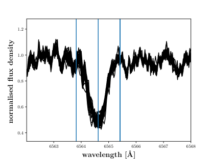
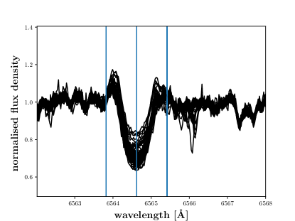
Figure 1: Two typical H$\alpha$ line profiles for our sample stars: BD+44 2051A (left panel), one of the least active stars and V2689 Ori (right panel), the most active star in our sample. All usable spectra of the two stars are shown to demonstrate that the chromospheric line shows relatively small variations. The vertical lines correspond to the borders of our central wavelength interval.

To quantify the scatter, we computed the median average deviations (MADs), which is a robust estimate somewhat similar to the standard deviation (Rousseeuw & Croux, 1993; Czesla et al., 2018), for H$\alpha$, the bluest line of the Ca ii IRT, and the blue Na i D line. The level of variability in the H$\alpha$ and the Ca ii IRT lines is well correlated and is consistent with low activity levels. In contrast, the correlation between the MADs of the Ca ii IRT and Na i D is non-significant. While the MAD(Na) is normally equal or lower than the MAD(Ca), for Lalande 21185 this is not the case. In general, H$\alpha$ shows the highest degree of variability, followed by the Ca ii IRT lines, while Na i D is the least variable.

To study the mutual relation between the behaviour of the individual activity indicators, we compute Pearson’s correlation coefficient obtained from the time series (with the flare spectra being excluded) and give the values in Table 3. Values not significant at the 1  % level are shown in square brackets. In particular, we relate $I_{\rm H\alpha}$ to $I_{\rm Ca,1}$ and $I_{\rm Na}$ and also investigate the correlation coefficient corresponding to the first and second Ca ii IRT lines and between the two lines of the Na i D doublet.

As expected, the indices of the individual Na i D doublet lines are correlated with each other; similarly, the two bluer Ca ii triplet lines are significantly correlated in all stars. The correlation between $I_{\rm{H}\alpha}$ and $I_{\rm Ca,1}$ is also strong for the majority of the sample stars and remains non-significant in only four of them, which are all among the least active according to their median $I_{\rm Ca,1}$ index. We attribute the lack of a significant correlation to the low level of variability in these stars and our resulting lack of sensitivity rather than a physical mechanism. All significant correlation coefficients are positive and rather large with seven exceeding $0.8$, which indicates a similar response of these two indices to changes in the activity level.

The rate of significant correlation coefficients between $I_{\rm{H}\alpha}$ and $I_{\rm Na,1}$ is lower compared to the previous comparison with $I_{\rm Ca,1}$. Only five stars show a significant correlation between these indices, and whenever it is significant, the coefficient is always lower than for the correlation between $I_{\rm{H}\alpha}$ and $I_{\rm Ca,1}$. While this result may also be partially explained by a lack of sensitivity, which would have to affect primarily the $I_{\rm Na,1}$ index, this argument is certainly inapplicable in the case of V2689 Ori, which shows detectable variability in all studied indices. We attribute the correlation coefficients with lower significance and the high rate of non-significant values to differences in chromospheric activity in the different line-formation regions, that is, the higher chromosphere in the case of H$\alpha$ and the lower chromosphere for the Na i D doublet (Andretta et al., 1997).

For the two stars AN Sex and V2689 Ori, for which we excluded the highest number of flaring spectra (4 and 14, respectively), we also computed the correlation coefficient between $I_{\rm{H}\alpha}$ and $I_{\rm Na,1}$ including the flaring spectra. In this case, we found significant correlation coefficients of $0.53$ for AN Sex and $0.79$ for V2689 Ori. This result is driven by the flare spectra and shows that strong changes in the activity level are similarly traced by both lines.

4.3 Alternative indices and robustness

To study the impact of the index definition on the results, we introduce alternative indices for the H$\alpha$ and the bluest Ca ii IRT line. This allows us to test, for example, whether or not the width of the central wavelength interval influences the period analysis. To this end, we define four alternative indices, which we dub A1–4. Specifically, we use (i) the pseudo equivalent width (pEW) of the H$\alpha$ line based on a central wavelength band of 6563.9 – 6565.5 Å, referred to in the following as A1 pEW; (ii) a pEW covering only the core from 6564.4 – 6564.85 Å  (A2 pEW); (iii) a pEW with broader central wavelength range of 6560 – 6570 Å  (the latter would account for flares – A3 pEW); and (iv) a pEW with variable central bandwidth which is defined by the foot points of the line (A4 pEW). For these pEW time series we used three-sigma clipping to exclude flares and other outliers.

The variable pEW measurements (A4 pEW) rely on locating the maxima and minima in the ranges 6563.6 to 6564.4 and 6564.85 to 6565.7 Å. The minimum values form the range for A4 pEW and the maximum values are used to calculate the pEW of the H$\alpha$ central reversal in stars that have H$\alpha$ in emission. All pEW(A1-A4) use the reference regions of 6550 to 6555 and 6576 to 6581Å, which are different from the reference regions used for $I_{\rm{H}\alpha}$. However, also for A1 to A4, none of the spectra were corrected for tellurics as the used regions have only very weak telluric lines. These weak lines have an influence on the resultant pEW, which is significantly less than the margin of error.

Of these alternative indices, A1 is most similar to $I_{\rm{H}\alpha}$; only the reference bands differ and the method of calculation (integral instead of mean).

Table 3: Measured activity properties of our sample stars.

Name	No.	No.	Median	Median	Median	Corr	Corr	Corra	Corrb	MAD	MAD	MAD
	spec	spec	($I_{\rm{H}\alpha}$)	($I_{\rm Ca,1}$)	($I_{\rm Na,1}$)	H$\alpha$ -	H$\alpha$ -	Ca -	Na -	H$\alpha$	Ca	Na
	Na D	flare	[Å]	[Å]	[Å]	Ca	Na	Ca	Na	[$10^{-2}$]	[$10^{-2}$]	[$10^{-2}$]
GX And	145	1	0.37	0.27	0.45	[-0.026]	[-0.144]	0.55	0.96	0.6	0.1	0.2
BD+61 195	37	3	0.31	0.18	0.40	0.96	0.60	0.99	0.87	3.0	0.7	0.4
BD+21 652	114	0	0.62	0.25	0.45	0.75	0.38	0.91	0.93	0.8	0.3	0.2
BD+52 857	58	0	0.52	0.20	0.43	0.83	[0.29]	0.96	0.85	1.4	0.5	0.3
HD 36395	65	1	0.46	0.21	0.42	0.96	0.37	0.98	0.87	2.9	0.8	0.4
V2689 Ori	35	14	0.16	0.08	0.41	0.91	[0.46]	0.96	0.88	3.0	0.8	0.2
HD 79211	53	0	0.51	0.20	0.43	0.73	[0.01]	0.97	0.78	1.1	0.4	0.2
BD+63 869	26	0	0.48	0.20	0.43	0.93	0.65	0.97	0.86	1.8	0.6	0.3
AN Sex	25	4	0.34	0.20	0.40	0.90	[0.09]	0.95	0.86	1.5	0.4	0.3
Lalande 21185	145	2	0.27	0.27	0.46	[-0.16]	[-0.12]	0.31	0.98	1.1	0.2	0.5
BD+44 2051A	99	1	0.33	0.27	0.46	[-0.09]	[-0.24]	0.83	0.86	1.1	0.3	0.3
BD+11 2576	19	2	0.48	0.25	0.43	0.42	[0.09]	0.87	0.75	1.1	0.2	0.1
HD 119850	107	0	0.45	0.26	0.43	[0.14]	[0.19]	0.86	0.81	1.3	0.2	0.1
HD 147379	71	0	0.60	0.23	0.44	0.89	0.35	0.98	0.45	0.8	0.3	0.1
HD 199305	90	2	0.46	0.23	0.43	0.66	[-0.05]	0.93	0.83	1.0	0.3	0.1
HD 216899	115	3	0.42	0.22	0.42	0.76	[-0.05]	0.91	0.94	1.5	0.3	0.3

Note: The Pearson correlation coefficients given in square brackets have a corresponding p-value higher than 0.01.
^a: The correlation between $I_{\rm Ca,1}$ (at 8500.35 Å) and $I_{\rm Ca,2}$ (at 8544.44 Å).
^b:The correlation between the indices of the two Na i D lines.

5 Period search

5.1 Methods

We use several methods to search for periodic variations in the the previously defined time series of activity indices. Since the CARMENES data are not evenly spaced, some widely used period-search algorithms, such as many variants of Fourier transforms (FT), are not applicable. Here we focus on the following methods: Generalized Lomb-Scargle (GLS) periodogram, phase dispersion (PD) minimisation, string length (SL) method, and Gaussian process (GP) modelling with quasi-periodic kernel – hereafter referred to as GP.

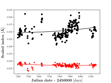
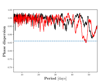
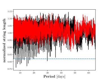
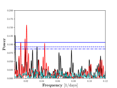
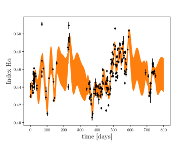
Figure 22: Results for HD 119850 as explained in Fig. 10.

Before the index time series are analysed, we detrend them (flare spectra excluded) using a second-order polynomial fit. This procedure yields a reasonable correction of long-term trends for most time series. A notable exception is the H$\alpha$ time series of HD 119850, which shows a complex evolution as shown in Fig. 22. This procedure also possibly suppresses periodic variations due to activity cycles on scales of years and beyond the observed timescale, to which we are therefore not sensitive. Detrending is not used for the GP analysis, for which it is not required.

Generally, we search for periods between 1 and 150 days, with the lower limit given by the observing scheme, which normally does not lead to more than one observation per night, and the upper limit suggested by the length of one observing block introduced by the seasonal visibility of the objects.

5.1.1 Generalized Lomb-Scargle periodogram

We use the generalized Lomb-Scargle (GLS) periodogram as implemented in PyAstronomy (Zechmeister & Kürster, 2009; Scargle, 1982; Lomb, 1976) to compute periodograms for the index time series of H$\alpha$, the bluest Ca ii IRT line, and the bluer Na i D line, adopting the normalisation to unity introduced by Zechmeister & Kürster (2009) in their Eq. 4. In the case of H$\alpha$, we consider the four different pEWs introduced in Sect. 4.3 to study the impact of the definition. Along with the periodograms, we derive false alarm probability (FAP) levels of 10, 5, and 1 % and also the window function. In our analysis, we consider only peaks with power values exceeding the 1 % FAP level. A typical example of a GLS periodogram is shown in Fig. 2 for the star V2689 Ori. While the main power peak of the H$\alpha$ time series is significant, the one for Ca ii IRT is not. Both agree well with the literature value for the period of 12.3 days (Díez Alonso et al., 2018). In H$\alpha$ a (non-significant) peak is seen also at half the frequency (or twice the period) indicating the importance of harmonics for this star.

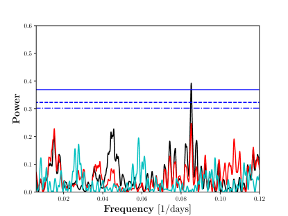
Figure 2: A representative GLS periodogram, here for the star V2689 Ori. While the horizontal dashed lines mark the 10 (blue/dot-dashed), 5 (blue/dashed), and 1 % FAP levels (blue/solid), the power is given in black for $I_{\rm H\alpha}$ and in red for $I_{\rm Ca,1}$. The cyan line denotes the window function.

5.1.2 Phase dispersion minimisation and string length method

The phase dispersion minimisation and string length methods are both based on phase folding the time series with a series of trial periods and analysing the folded time series. The basic idea is that the phased time series shows a well defined ‘curve’ only if the data are folded with the correct period that is also present in the data. This rather intuitive ansatz can be quantified by measuring (i) the length of the line connecting all data points, the so-called string length, $L$, (Dworetsky, 1983) or (ii) the variance of the folded time series estimated in several phase bins compared to the sample variance, $\Theta$ (Stellingwerf, 1978). Both quantities are minimised when the trial period matches the period of a signal. The advantage of both of these methods is that they do not rely on specific functional forms of the signal (such as sine waves in the case of GLS) or equidistant sampling.

To compute the phase dispersion minimisation (PDM) statistic, $\Theta$, as a function of a trial period, we use the implementation provided by PyAstronomy, which is based on the method introduced by Stellingwerf (1978). The investigated trial periods range from 1 to 150 days with an increment of 0.05 days. Each phase diagram is then divided into ten bins and three phase-shifted bin-sets are used to estimate $\Theta$.

For computing the string length, $L$, we fold the index time series with 20 000 trial periods between 1 and 150 days. Prior to folding, we re-scaled the data following the procedure by Dworetsky (1983). For each trial period, we compute the resulting string length and, finally, both $\Theta$ and $L$ are normalised by their median values to facilitate an easier comparison between the different indices used. We dub the resulting statistics $\Theta_{n}$ and $L_{n}$.

We applied both methods to investigate the index time series of H$\alpha$, the bluest Ca ii IRT line, and the blue Na i D line. To identify appropriate FAP levels, we applied a bootstrap procedure. In particular, we randomly shuffle the index time series 10 000 times, which should destroy any temporal coherence, and compute new values of $\Theta_{n}$ and $L_{n}$, respectively. Based on their resulting distributions, we defined 1 % FAP levels, which are tabulated for each star in Table 4 and are used as cut-off in our analysis.

To identify the significant periods, we visually inspected the diagrams and screened them for dips exceeding the previously defined cut-off. It appears that both methods are rather prone to aliasing, that is, they yield peaks at frequency multiples of the (unknown) true period, which complicates the interpretation of the resulting string length and phase dispersion diagrams. If more than one dip exceeding the 1 % FAP level was found, we picked the most pronounced and also report the second in strength. Only when a series of likely aliases was detected, did we opt for the smallest period in this series, even if this did not correspond to the peak with the highest formal significance. If this peak did not reach the 1 % FAP level we give it in square brackets in our results in Tables 5 and 6.

Table 4: Monte Carlo simulated values of string length or phase dispersion corresponding to 1 % FAP for each star.

Star	$L_{n}$ cut off	$\Theta_{n}$ cut-off
GX And	0.85	0.88
BD+61 195	0.69	0.70
BD+21 652	0.78	0.86
BD+52 857	0.70	0.73
HD 36395	0.74	0.77
V2689 Ori	0.65	0.60
HD 79211	0.78	0.79
BD+63 869	0.67	0.66
AN Sex	0.72	0.69
Lalande 21185	0.82	0.88
BD+44 2051A	0.73	0.77
BD+11 2576	0.72	0.69
HD 119850	0.82	0.86
HD 147379	0.76	0.83
HD 199305	0.77	0.84
HD 216899	0.81	0.88

As an example, we show the computed string length and the phase dispersion for V2689 Ori in Fig. 3. For this specific light curve the double, triple, and even quintuple of the known period of 12 days actually produce a lower string length than the true period. For Na i D the correct period is not found, while the alias corresponding to twice the actual period is detected. The string length and phase dispersion curves for all stars are found in the Appendix.

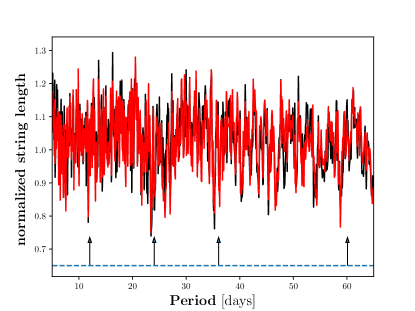
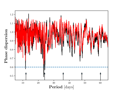
Figure 3: ”Representative string length (top) and phase dispersion (bottom) diagrams for the star V2689 Ori. The black line denotes the computed $L_{n}$ and $\Theta_{n}$ for $I_{\rm H\alpha}$, respectively. The red line denotes $L_{n}$ and $\Theta_{n}$ for $I_{\rm Ca,1}$, respectively. The blue dashed horizontal line denotes the 1 % FAP level below which a period would be significant. The arrows mark the photometrically measured period of 12.02 days (Kirkpatrick et al., 2012) and multiples.

5.1.3 Gaussian process regression with quasi-periodic kernel

A Gaussian process (GP) consists of sets of random variables of which any finite set has a joint normal distribution (Rasmussen & Williams, 2006). A GP is completely specified by a mean and a co-variance function, and the latter can be used to search for periodic variation. The actual distribution of the errors in the data is rarely known. Nonetheless, the assumption of normality is often very helpful and appropriate in data modelling (e.g. Jaynes, 2003), which makes GPs a highly valuable tool for data analysis. At the heart of GP modelling lies the chosen kernel function, which describes the co-variance of the data. The choice of kernel is essentially ad hoc and depends on the data to be modelled.

Rasmussen & Williams (2006) use the product of a squared exponential and a periodic kernel to model the temporal variation of the CO₂ concentration measured in Hawaii. Here the squared exponential term accounts for secular variation and the periodic term describes the seasonal modulation. The construction of the kernel is such that a decay away from strict periodicity is allowed.

Angus et al. (2018) use this kernel to model rotational stellar variability in photometric time series. Again, the kernel accounts for a periodic term, in this case caused by spot-induced variation, superimposed on a long-term secular evolution. The periodic term here accounts for spot-induced rotational variation while the squared exponential term models long-term changes in the activity state.

The main difficulty in GP modelling is due to the fact that the co-variance matrix of the data needs to be inverted many times; for large data sets containing thousands of data points this is a true challenge. For our analysis we use the python interface of the celerite algorithm, which is capable of highly efficiently carrying out a GP regression in one dimension (Foreman-Mackey et al., 2017). We use a co-variance function of the form

$$k(t_{n},t_{m})=\frac{a}{2+b}e^{-c\tau}\left[\cos\left(\frac{2\pi\tau}{P}\right)+(1+b)\right]+\delta_{nm}\sigma^{2}\;,$$ (2)

where $\tau=|t_{n}-t_{m}|$ and $t_{i}$ denotes the individual points on the time axis. This choice corresponds to the proposal by Foreman-Mackey et al. (2017) in their Eq. 56, extended by a “jitter” term, that is, additional, normally distributed white noise. The co-variance function requires that all of the parameters $a,b,c$, and $P$ are positive. The Foreman-Mackey et al. (2017) kernel is characterised by an exponential decay on timescale $\tau$ and includes a periodic term with a period, $P$, and a secular term. The amplitude of the co-variance and the relative impact of the periodic and secular terms are determined by combinations of the values of the parameters b and c. This Foreman-Mackey et al. (2017) kernel is similar (but not identical) to the one used by Rasmussen & Williams (2006) and Angus et al. (2018).

In our modelling, the four parameters $a,b,c$, and $P$ are varied to find the maximum of the likelihood function, which is accomplished using the “limited memory Broyden-Fletcher-Goldfarb-Shanno with box constraints” (L-BFGS-B) algorithm, an iterative optimisation algorithm belonging to the group of the quasi-Newton methods, as implemented in SciPy (Jones et al., 2001).

Some value for the period, $P$, will always maximise the likelihood; however, this does not automatically imply that it is reasonable to consider this value in a physical interpretation. This brings us into the realm of hypothesis testing. As an alternative to the periodic co-variance function as specified by Eq. 2, we can set up a hypothesis without any periodic behaviour. The periodic term in Eq. 2 is suppressed if the period $P$ is large or, for that matter, infinitely long. Taking the limit, Eq. 2 then becomes

$$k(t_{n},t_{m})=ae^{-c\tau}+\delta_{nm}\sigma^{2}\;.$$ (3)

The relative plausibility of these hypotheses is expressed by the posterior odds, which is equivalent to the Bayes factor if impartial prior odds are assumed. Evaluating the Bayes factor requires a numerical value for the marginal likelihoods to be obtained, which is usually a troublesome enterprise. However, it can be shown that the so-called Schwarz Criterion,

$$S=\max(\mathcal{\log\,L}_{1})-\max(\mathcal{\log\,L}_{2})-\frac{1}{2}d\log\,n,$$ (4)

which asymptotically approximates the Bayes factor (e.g. Kass & Raftery, 1995). Here, $\max(\log(\mathcal{L}))$ denotes the maximum of the (logarithm of the) likelihood function under the respective hypothesis, and $d$ represents the difference in dimensionality, which we take to be two in our case, and $n$ is the number of data points for the specific star. A value of about zero for $S$ translates into posterior odds of around one. In that case, the data provide similar support for both hypotheses. Positive $S$ indicates support for the periodic model in our case. At which point to accept the periodic hypothesis depends on the assumed loss associated with a false decision. We here adopt a conservative limit of $\log(S)=4.6$, which corresponds to posterior odds of $100:1$ in favour of the periodic term. In Tables 5 and 6 we report the resulting periods. Values in agreement with the results of other methods but unacceptable according to our criterion are given in square brackets. The $S$ values are provided in Table 7.

As an example, we show our GP modelling of the H$\alpha$ index time series of V2689 Ori along with the maximum-likelihood predictions for the mean and standard deviation in Fig. 4. Moreover we show in blue the best model prediction with the non-periodic kernel. This example demonstrates the ability of the model to account for more complicated long-term trends, which do not have to be removed before applying the method. In the Appendix we show similar graphs for all stars.

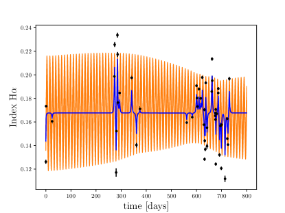
Figure 4: H$\alpha$ time index series of V2689 Ori (black data points) along with maximum a posteriori GP model prediction and standard deviation indicated by orange/light grey shade. In blue/dark grey the best GP model without periodic term.

5.2 Results

Naturally, the period search outcomes provided by the various techniques differ somewhat. We claim a solid detection of a periodic signal in a specific star, if we find the same period with at least four of the methods (SL, PD, GLS, GP, GLS and GP applied to the alternative index A1) allowing for a margin of 10 % in the numerical value of the period. A tentative period is reported in square brackets if the same period is found using three methods (allowing also for tentative detections given in brackets). Otherwise, we consider the signal to be non-significant.

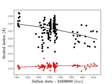
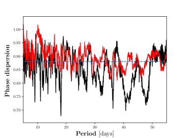
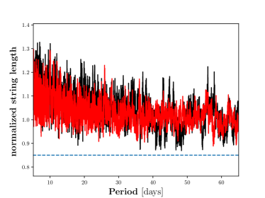
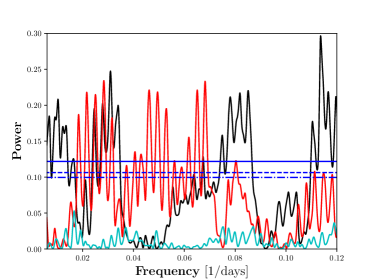
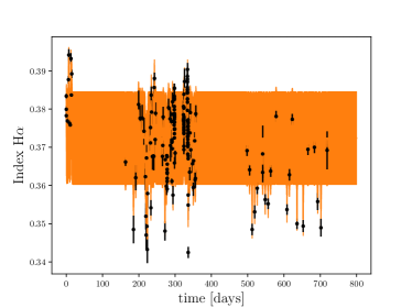
Figure 10: Results for GX And. Top left: Index time series in black dots for $I_{\rm{H}\alpha}$ and in red asterisks for scaled $I_{\rm Ca,1}$. The corresponding solid lines represent the best second-degree polynomial fit. Top right: Phase folded index time series of $I_{\rm{H}\alpha}$ (only present in case we found a period using H$\alpha$). Second row left: Phase dispersion minimisation. The black line denotes $\Theta$ computed for $I_{\rm{H}\alpha}$, while the red line denotes $\Theta$ for $I_{\rm Ca,1}$. The dashed horizontal line marks the 1 % FAP level. Second row right: String length method. Again, the black line denotes the string length $L$ for $I_{\rm{H}\alpha}$ and the red line is also the string length but computed for $I_{\rm Ca,1}$. Third row left: GLS periodogram with FAP levels of 10 %, 5 %, and 1 % in blue (dash-dotted, dashed, and solid), respectively. In the periodogram the black line denotes the normalised power calculated with $I_{\rm{H}\alpha}$, while the red line again is the power of $I_{\rm Ca,1}$, and the cyan line the window function. Third row right: Index time series of the H$\alpha$ indices with the GP best-fit model in orange and its standard deviation shaded in light orange.

According to this criterion, we report a solid detection of a periodic signal in four out of the 16 sample stars based on the H$\alpha$ index and in five stars using the Ca ii IRT index. The GLS periodogram and GP were applied to the line index and the alternative indices defined in Sect. 4.3 Our results are summarised in Table 5 for the H$\alpha$ indices and in Table 6 for the Ca ii IRT indices. We also give an error estimate for the mean periods computed as the standard deviation of the mean of the different methods. In addition to the found periods we give the difference $\delta P_{\rm lit}$ to the literature period values given in Table 1. In all cases, we find agreement between our periods and those previously reported to within 3$\sigma$. Corresponding to the GP modelling we give the Schwarz criterion $S$ in Table 7. For all of our sample stars using the H$\alpha$ line index we show the GLS periodogram, the string length and phase dispersion distributions, and the modelling of the GP in the Appendix (Figs. 10 to 25).

All measured periods using the H$\alpha$ and Ca ii IRT indices agree to within 2$\sigma$. This is also the case for the three stars HD 79211, AN Sex, and BD+11 2576 where we found tentative periods with both H$\alpha$ and the Ca ii IRT indices. Although many methods do not find the period with the demanded significance, the finding of the same period in two different indices strongly suggests that this is the correct period. The case is different for the stars BD+52 857 and HD 216899 where a tentative period is found only in the Ca ii IRT indices but not in the H$\alpha$ line indices. Nevertheless, the tentative period of HD 216899 is in agreement with the literature value.

For the stars HD 79211, BD+63 869, and HD 147379 we could derive previously unknown rotation periods, with HD 79211 being a tentative detection and HD 147379 being detected only in Ca ii IRT.

For the three stars BD+61 195, HD 36395, and BD+63 869 consideration of the H$\alpha$ and Ca ii indices and nearly all methods led to the individual period. For V2689 Ori and AN Sex the same applies, except that we found the same period or multiples thereof with all methods, and not every method reached the significance threshold (though gave the right period). These five stars are among the most active in our sample as measured by their median $I_{\rm Ca,1}$ index. Not surprisingly, they are also the most variable as, for example, measured by the MAD of $I_{\rm{H}\alpha}$. These stars are members of the young disc population with the only exception being HD 36395, which is classified as a thin disc member.

For GX And, Lalande 21185, and BD+44 2051A the algorithms in our analysis had the lowest success rate in finding periods. These three stars are the least active in the sample according to their median $I_{\rm Ca,1}$ index. Expectedly, they are also among the least variable ones as measured by the MADs of $I_{\rm Ca,1}$ and $I_{\rm{H}\alpha}$ (Table 3). All three stars are members of the disc or the thick-disc populations (Table 1). In contrast to the cases of Lalande 21185 and BD+44 2051A, our period search in GX And failed because it shows many formally significant periods instead of none. This behaviour is caused by the special temporal sampling with many observations taken on a single night and is discussed in more detail in Sect. 6.4.

For four stars with detected periods, we have also computed expected (maximum) periods from the rotational velocity (see Table 1). For V2689 Ori and HD 79211 the expected period is slightly smaller than the measured period. For HD 147379 we find twice the expected period, which could indicate that by using chromospheric indicators we actually detected an alias of the true period. In the case of BD+21 652, we recover the photometrically measured period, which is, however, about four times larger than the one based on the projected rotation velocity, which we attribute to the uncertainty of the $v\sin i$ value. Lowering $v\sin i$ by two standard errors reconciles the values, which appears statistically plausible.

The stars Lalande 21185 and HD 119850 have known spectroscopically determined periods, which we could not recover.

We attribute this to their low activity levels and the resulting low variability amplitudes. A spectroscopic rotation period has also been determined using the Ca H and K lines and the H$\alpha$ line for HD 216899 (Suárez Mascareño et al., 2015). For this star we find only a tentative period and this only in $I_{\rm Ca,1}$. Since the star is not as inactive as the preceding two, we are probably not limited by sensitivity in this case. Instead, a change in the surface spot configuration provides a possible explanation for the lack of a detection in our data set.

Table 5: Results of the different period search methods for each star using H$\alpha$.

Star	SL	PD	GLS	GP	GLS A1	GP A1	Found period	$\Delta P_{\rm lit}$
	[d]	[d]	[d]	[d]	[d]	[d]	[d]	[d]
GX And	94.9,86.4	many	many	…	many	…	no period	…
BD+61 195	18.9	18.8	18.8,18.3	18.8	18.9	18.8	18.8 $\pm$ 0.2	0.4, 1.1
BD+21 652	…	50.5	24.3,25.5,27.7	[24.5]	56.6,25.1	[25.0]	[25.3$\pm$ 1.1]	0.1
BD+52 857	…	…	28.3,23.8,22.2	…	16.5,19.9	…	no period	…
HD 36395	…	33.4	34.0	34.1	34.1,33.9	33.9	33.9 $\pm$ 0.4	0.1, 0.3
V2689 Ori	[11.8]	11.7, 23.4	11.8	11.8	12.2,11.7	11.7	11.8 $\pm$ 0.2	0.2, 0.5
HD 79211	…	52.3, [16.7]	23.6,33.3	[17.4]	16.5	[16.4]	[16.6 $\pm$ 0.5]	…
BD+63 869	17.8	17.8	17.8	17.8	17.7	17.8	17.9 $\pm$ 0.3	…
AN Sex	…	[21.4]	21.3	[21.7]	21.3,17.9	[19.4]	[20.1 $\pm$ 1.5]	1.5, 1.5
Lalande 21185	5.8,7.9	97.5	150	…	…	…	no period	…
BD+44 2051A	…	…	…	…	…	…	no period	…
BD+11 2576	30.7	30.7	[31.3]	[31.0]	…	…	[30.8 $\pm$ 0.3]	2.8
HD 119850	many	88.8	…	…	46.2,51.4	…	no period	…
HD 147379	…	73.2	…	[21.9]	20.8	[21.5]	no period	…
HD 199305	…	…	…	…	…	…	no period	…
HD 216899	…	89.2,39.1	…	…	18.3,19.2	…	no period	…

Table 6: Results of the different period search methods for each star using Ca ii IRT.

Star	SL	PD	GLS	GP	GLS A1	GP A1	Found period	$\Delta P_{\rm lit}$
	[d]	[d]	[d]	[d]	[d]	[d]	[d]	[d]
GX And	…	…	many	…	many	…	no period	…
BD+61 195	[18.9]	18.8	18.8,18.3,20.4	18.7	18.9	18.9	19.1$\pm$0.7	0.8,0.7
BD+21 652	137.2	27.6, 27.4	27.7 +sidemax	24.7	25.6	[25.4]	25.9$\pm$1.0	0.5
BD+52 857	…	69.9,22.0,15.8	22.2,23.8,28.3	16.7	30.3	[16.7]	[16.5$\pm$ 0.3]	…
HD 36395	33.4,34.2	34.1	34.3	34.3	34.5	34.3	34.1$\pm$ 0.5	0.3, 0.5
V2689 Ori	[11.8]	[11.7]	[11.8]	11.8	11.8	12.2	[11.9 $\pm$ 0.2]	0.4, 0.1
HD 79211	…	49.6,29.4	16.9,23.8	[19.3]	18.1	[17.1]	[17.4$\pm$1.0]	…
BD+63 869	17.8	17.7	17.8	17.9	17.7	17.8	17.8$\pm$ 0.1	…
AN Sex	…	21.3	21.3, 10.7	[21.9]	21.3,10.7	[22.0]	[21.1 $\pm$ 0.4]	0.5, 0.5
Lalande 21185	97.5	…	20.2	…	…	…	no period	…
BD+44 2051A	…	137.9	…	…	…	…	no period	…
BD+11 2576	…	30.1	[30.3,62.5]	…	[30.5]	[30.3]	[30.3$\pm$] 0.2	2.3
HD 119850	…	47.9	48.3	…	…	…	no period	…
HD 147379	…	20.9	21.3	21.6	21.3	21.4	21.4$\pm$ 0.4	…
HD 199305	…	53.1	…	…	…	…	no period	…
HD 216899	38.7	89.2,38.7,44.8	45.7	[40.1]	…	[40.6]	[39.2$\pm$0.4]	0.3,1.7

Table 7: Schwarz criterion $S$ for the GP modelling.

Star	$S_{I(H\alpha)}$	$S_{I({Ca\textsc{ii}})}$	SpEW(Hα)A1	SpEW(Ca)A1
GX And	-8.0	-6.4	-1.1	-2.9
BD+61 195	9.0	5.1	4.8	11.6
BD+21 652	-0.9	7.9	-0.5	3.2
BD+52 857	-5.5	4.8	-3.8	1.4
HD 36395	9.7	14.9	10.0	8.2
V2689 Ori	5.6	4.5	6.5	3.1
HD 79211	-4.6	-3.1	-1.8	1.4
BD+63 869	8.9	6.9	5.4	3.9
AN Sex	-4.1	-3.6	-2.6	-7.3
Lalande 21185	-3.2	-12.7	-4.8	-6.8
BD+44 2051A	-6.9	-3.8	-3.1	-3.1
BD+11 2576	-4.0	-3.0	-1.9	0.7
HD 119850	-5.5	-5.4	-5.2	-2.5
HD 147379	2.7	17.1	-0.2	14.8
HD 199305	-2.3	-2.9	-3.6	-4.9
HD 216899	-2.0	-1.5	-2.2	-1.2

In our analysis using GLS periodograms we also investigated the window function to identify frequencies with high power introduced by the temporal sampling of the observations. We did not find any significant peak in the power of the window function. The highest peak therein is around two days for many of our stars, which would lead to aliases around two days again for the found rotation periods. Therefore, the sampling seems to be no problem here.

While the period search based on the H$\alpha$ and Ca IRT lines provides encouraging results, the measurement of the rotation periods using the Na i D line indices turned out to be less successful. We elaborate on the possible reasons for this finding in Sect. 6.3. While the string length method and the phase dispersion minimisation perform worst for our sample, the GP modelling is the clear winner among the studied algorithms in terms of detection performance; see Sect. 6.7.

6 Discussion

6.1 Connection of activity properties to period finding

Since measurements of the rotation are only possible if the star exhibits a non-uniform pattern of H$\alpha$ or Ca ii plages that imprints itself in periodic variations in the EW of the chromospheric lines, it is not possible to measure rotation if the amplitude of these variations is not high enough. For the case of low- or medium-active stars the activity variations are not dominated by micro-flaring and other intrinsic variability, but should be dominated by plage evolution and rotation. Therefore the activity properties of the individual stars should provide some insight into whether or not it is probable that a period will be found.

Inspecting the median($I_{\rm Ca,1}$) we notice that for the seven stars with values of 0.21 or smaller there was always a period found (though for some stars only tentative or in only one index). For the four stars with values of 0.26 or higher we do not find a period. For the five stars with intermediate values, the situation is unclear. For the median($I_{\rm H\alpha}$), the situation is also unclear since it can vary quite a lot for the same values in median($I_{\rm Ca,1}$), which may be caused by different filling factors of plages and filaments. This is in line with the finding that for the three stars with the worst correlation between H$\alpha$ and Ca ii IRT indices we cannot establish a period.

Moreover, we could find a (tentative) period in all cases where the MAD(Ca) is 0.004 or higher. For the nine stars with a lower MAD(Ca) one may or may not find periods. Also, for the MAD(H$\alpha$) the situation is less clear but there is the tendency to find a period for high MAD(H$\alpha$), while for lower values finding a period becomes harder and harder. Interestingly the low correlation between H$\alpha$ and Ca ii IRT indices is only coupled to the lowest MAD in Ca ii as well as in H$\alpha$ only for GX And. If there is no variation, no correlation can be found either.

A period could be detected in all stars with a correlation between H$\alpha$ and Na i D. A correlation between these two lines, one formed in the upper chromosphere, the other in the lower chromosphere, may indicate plage configurations which are especially stable or of high contrast or both. For the low-activity stars in our sample it appears that a period is more likely to be found if the star is among the more active ones as measured by median($I_{\rm Ca,1}$), MAD(Ca), and MAD(H$\alpha$), since in these rather inactive stars the variability is probably dominated by rotational effects. In contrast, for the most active mid-type M dwarfs the opposite is expected, and the chances of finding a period are lower because flaring variability will dominate over rotational variability for these stars.

6.2 Comparing the width of the H$\alpha$ central wavelength band

Since the width of the H$\alpha$ line can vary a lot, different widths of the central waveband are used in the literature to account for this problem. We therefore investigate whether or not these different widths have an influence on the period finding.

In Fig. 5 we show a comparison using a GLS periodogram and no detrending of the data of BD+61 195. While the alternative pEW A1, the pEW with variable width A4, and the core pEW A2, all show high significance at the known period of $\sim$19 days, the pEW with the broadest central wavelength band (A3) does not. This lower performance of A3 is quite typical for the whole sample. Additionally it may lead to spurious peaks at periods higher than 100 days. A1 and A4 normally perform about equally well. The A2 core pEW shows quite different sensitivity to rotation and sometimes performs better, but also sometime much worse than the other two. This may be expected since it is more sensitive to smaller variations in H$\alpha$ which normally occur first in the core. This leads to a better performance of A2 in cases of variations caused by rotational modulation. We demonstrate this using the example of HD 119850 in Fig. 6. This star has a photometrically determined period of 52.3$\pm$ 1.3 days (Suárez Mascareño et al., 2015), but we do not find any period. The star is among the most inactive of our sample. We compare A2 and A1 with and without detrending. While using A1, the period is not found regardless of whether detrending is used, whereas in the A2 data a signal corresponding to the photometric period is clearly seen. Unfortunately, this does not work for the other very inactive stars, GX And, Lalande 21185, and BD+44 2051A.

Figure 5: Periodogram comparing the different central wavelength ranges of H$\alpha$ for BD+61 195. The pEW A1 is designated by the black line, the core pEW A2 is in green/dotted, the pEW with broad central wavelength range A3 is in cyan/dashed, and the pEW with variable width A4 is in red/dot-dashed. The horizontal blue lines show the FAP levels of 0.1 (dash-dotted), 0.05(dashed), and 0.01 (solid).

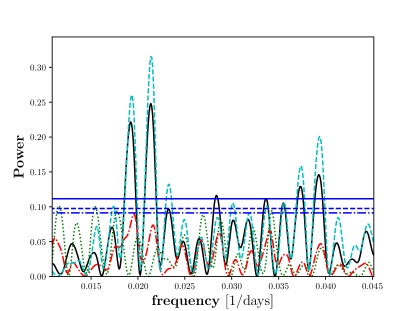
Figure 6: Periodogram comparing the central wavelength ranges of H$\alpha$ for HD 119850 and with and without detrending. The pEW with a width of 1.6 Å  is designated by the green/dotted line for no detrending and by the red/dash-dotted line in case of detrending. The pEW of the line core is in black/solid for no detrending and in cyan/dashed for detrending. The horizontal blue lines show the FAP levels of 0.1 (dash-dotted), 0.05 (dashed), and 0.01 (solid).

6.3 The Na i D lines

Besides H$\alpha$ and Ca ii, we considered the Na i D lines for our period search. For mid M dwarfs the Na i D lines are known to develop emission cores and are therefore clearly also sensitive to activity. A big obstacle in their usage for period analysis is the Na i D airglow lines. This terrestrial emission is variable in time and can be relatively strong. Therefore, we did not try to correct this emission, but we excluded all spectra from the analysis where the airglow may influence the central wavelength band of the Na i D line. Unfortunately this leads to rather small numbers of available spectra (see Table 3) for all stars where we found rotation periods besides BD+21 652. For this star the significance in the GLS periodogram for Na i D unfortunately stays below a FAP of 0.1 at the period found. One should nevertheless keep in mind that BD+21652 is a rather inactive star; in fact the most inactive star for which we could establish a period. Generally, the low correlation of H$\alpha$ and Na i D and the low MAD(Na) values may indicate that the Na i D line is not as sensitive to activity as H$\alpha$ and therefore could only be used for more active stars. For a more active star on the other hand, namely BD+61 195, where we have only 37 usable spectra for the Na i D periodogram computation, the highest peak is nearly significant as can be seen in Fig. 7. This may promise that for stars with higher activity level (as indicated e.g. by the MAD(Ca)) an analysis using Na i D can be accomplished once enough spectra not contaminated by airglow are available.

Figure 7: GLS periodogram for BD+61 195 comparing H$\alpha$ in black/solid, Ca ii IRT in red/dash-dotted, and Na i D in cyan/dashed. The horizontal blue lines show the FAP levels of 0.1 (dash-dotted) , 0.05 (dashed), and 0.01 (solid).

6.4 Influence of detrending, flaring activity, and multiple observations per night

The handling of detrending, flaring activity, and multiple observations per night is theoretically expected to potentially hinder the period search, since all three have a negative impact on the systematic ‘noise’ of the time series.

Regarding the detrending, it can be seen in Fig. 6 that detrending often leads to a higher significance of the period. In cases of weaker trends in the time series we do not, however, find an influence. Detrending may also lead to small shifts in the period, with the largest shift we found from 33.0 without to 34.2 days with detrending (in HD 36395). We conclude that detrending the data leads normally to an equally good or better performance of the GLS periodogram.

We want to make clear nonetheless that these trends removed by detrending are interesting in themselves as they may represent parts of activity cycles. Unfortunately the time baseline of the CARMENES data up to now is not long enough for a reasonable search of such long-period signals. If one looks at the index time series directly, striking examples of nearly linear trends in both $I_{H\alpha}$ and $I_{CaIRT,1}$ may be found in BD+52 857, BD+11 2576, and HD 147379, while BD+21 652, HD 36395, and V2689 Ori show more parabolic trends.

In the case of flaring one can test the sensitivity of the search algorithm with respect to outliers. For the star V2689 Ori we had to exclude a significant number (22 %) of spectra flagged as taken when the star was flaring. To infer how important the exclusion of such outliers is, we recomputed the period of the star using the different methods on the full index time series including the spectra flagged due to flaring activity. Surprisingly we could recover the period without problems. The string length and phase dispersion method both had the problem of heavy aliasing as when using the clipped index time series. The double period is found again significantly while even higher multiples and the period itself give lower significance. As an example we show the recomputed GLS in Fig. 8. Interestingly, the power computed including the spectra affected by flares shows a peak nearly as high as the power computed without them. For the Ca ii IRT this effect is even more remarkable since the highest peak becomes statistically significant with FAP ¡ 0.01 when including the flare spectra. This leads us to the hypothesis that for V 2689 Ori our flare criterion is not working well and instead a high amplitude in rotational variation triggers our flare criterion so that we exclude spectra not flaring but being the peaks in the rotational index time series. If one were to examine the index time series in Fig. 8 by eye, we would mark only three to four spectra as flaring – a number so low that we would expect the period search algorithms to work correctly despite these outliers.

Since V2689 Ori is our most active star and the only one where we flagged such a high number of spectra as flaring, we regard it a special case in our sample. However, this also leads to the conclusion that the flare criterion has to be defined with care.

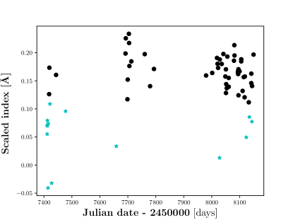
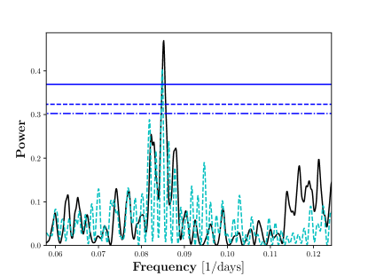
Figure 8: Influence of flaring spectra for V2689 Ori. Top: Index time series of $I(H\alpha)$ with (cyan) and without (black) flare-flagged spectra. Bottom: Comparison of the GLS with inclusion of flare-contaminated spectra (cyan/dashed) and without (black/solid). The horizontal blue lines show the FAP levels of 0.1 (dash-dotted) , 0.05 (dashed), and 0.01 (solid).

Having examined the influence of detrending and flaring, we now discuss multiple observations on single nights. Such observations may be problematic, if the star is intrinsically variable on short timescales and especially if the amplitude of these changes in the chromospheric lines are of the same order as the rotational changes. All stars have at least one night when more than one spectrum was taken as given in Table 1, but for most of the stars this is a minor aspect, and so intrinsic variability can again be seen as a small number of outliers. On the other hand, we have one extreme case in our sample: GX And with more than half of the spectra taken on only a few nights and up to 22 spectra taken on one night. Since for this star intra-night variations are easily noticed, the questions arises of whether this flickering has an amplitude hampering the period analysis. We therefore recomputed our period analysis after removing all spectra but one from each night with multiple observations, maintaining only the spectrum with the median H$\alpha$ index. Figure 9 shows the comparison between the analyses including multiple observations per night, and those using only single observations, for the GLS periodogram for GX And and for the more typically behaving star BD 21652 (which is nevertheless among the four stars with many multiple observations on single nights).

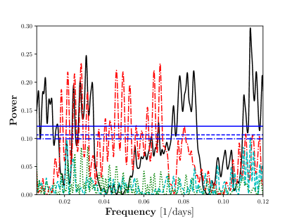
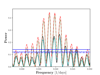
Figure 9: Influence of multiple spectra taken on one night on the GLS periodogram. Black/solid and red/dash-dotted denote the power for $I_{\rm{H}\alpha}$ and $I_{\rm Ca,1}$, respectively, including multiple spectra. Cyan/dashed and green/dotted denote the power for $I_{\rm{H}\alpha}$ and $I_{\rm Ca,1}$, respectively, excluding multiple spectra. The horizontal blue lines show the FAP levels of 0.1 (dash-dotted) , 0.05 (dashed), and 0.01 (solid). Top: The extreme case of GX And. Bottom: The typical case of BD 21652.

The GP is slightly more affected in analyses using multiple spectra from one night. For the majority of stars, the period stays the same or is only shifted by less than 5 % when the multi-observations are removed. Nevertheless, instead of the period of V2689 Ori, the threefold multiple is found and for the two stars BD 52857 and GX And significant periods of 21.8 and 46.2 days are measured if the multiple observations on single nights are excluded.

6.5 Comparison to other algorithms

There is ample literature on period searching and many algorithms have been introduced accordingly. Below, we discuss two variations of the methods tested here, which have shown promising results in previous studies.

The first is the conditional entropy (CE) algorithm by Graham et al. (2013a), which has been shown to perform well in a variety of astrophysical period-finding problems (Graham et al., 2013b). The CE algorithm belongs to the family of phase-folding algorithms and is thus related to the string length and the phase dispersion algorithms. The specific idea here is to arrange the data in a unity square of phase and normalised variation and quantify the degree of order in the resulting distribution via CE, which is to be minimized. We tested this algorithm on our $I_{\rm H\alpha}$ data using the same significance criterion as for the string length method. We were able to recover the periods of BD+61 195, HD 36395, and BD+63 869. We also found periods consistent with our previous results for BD+21 652, V2689 Ori, BD+11 2576, and HD 216899; however, these findings remained formally insignificant. Moreover, a significant period of 145 days was detected for Lalande 21185, which did not show up earlier in our analysis. The CE method clearly shows a sensitivity profile, that is similar but not identical to those of the string length and phase dispersion minimisation algorithms. On our data set, we found the performance of the CE method to be comparable to that of the string length and the phase dispersion algorithms. We note, however, that superior performance may still be achieved in other problems such as those studied by Graham et al. (2013b).

Secondly, we test the performance of a different quasi-periodic kernel in the GP modelling. In particular, we apply the kernel also adopted by Angus et al. (2018) in their periodicity study of Kepler light curves. Here we used the python module george, because this kernel cannot be combined with the fast matrix-inversion method applied by celerite. Based on the H$\alpha$ data and the alternative kernel, we could reproduce all periods found with celerite with the exception of those for V2689 Ori and AN Sex. Three periods identified tentatively using celerite, namely those for BD+21 652, HD 79211, and HD 147379, showed up as significant using the alternative kernel. Moreover, a significant period of 50.5 days was found for HD 119850, where we were not previously capable of assigning a period, although a spectroscopically determined period of 52.3 days is known (Suárez Mascareño et al., 2015). For the Ca ii IRT data the situation is similar: the period for HD 119850 was reproduced again, the periods for V2689 Ori and AN Sex were not found, for HD 216899 half the period showed up significantly, and for HD 36395 a period neither consistent with our previous results nor with the literature was found, which we consider likely spurious. Again, we conclude, that the results do not allow us to claim superiority for one or the other kernel. In fact, the two kernels perform similarly well but show an individual sensitivity profile on our data set.

At least as far as our data are concerned, the above results indicate that the concept behind the algorithm affects their performance more strongly than the details of their implementation. However, as shown for instance by Graham et al. (2013a), more pronounced differences may well show up when other data sets are studied. Therefore, we caution that this conclusion is not generally applicable.

6.6 Comparison to another CARMENES study

Schöfer et al. (2018) studied activity indicators for 332 M stars of the CARMENES sample. The main focus was on the question of which line indices could be used best as activity indicators and which ones are also suited for period searches. Therefore, using a GLS periodogram and different line/molecular indices in the optical and infrared a period search was conducted for 154 stars with known periods. More than 10 % of the known periods could be recovered using the molecular indices of TiO 7050 Å  and TiO 8430 Å, H$\alpha$, and the second line of the Ca ii IRT. The bluest and the reddest lines of the Ca ii IRT were used with less success, as were the Na i D lines and a number of other indices for chromospheric active lines. Nevertheless, a direct comparison to our study shows that of the four periods we found in H$\alpha,$ all were detected in the GLS periodogram and all were also found by Schöfer et al. (2018). For the blue line of the Ca ii IRT they recover periods for all stars where we also found periods besides BD+61 195. Therefore our results agree quite well with Schöfer et al. (2018) for the stellar sample used here, though they used a quite different definition of the activity indices with a  broad central wavelength range of 5 Å  in combination with the subtraction of the spectrum of an inactive star.

6.7 Comparison of the methods

To determine which of the methods used here works best, we counted (i) the false positive detections, which are either detections where no (tentative) period was assigned in the end or the values of the detected periods were not within 10 % of the assigned period (also counting double and half periods) and (ii) period non-detections where in the end a (tentative) period was assigned. The numbers of false positives and of non-detections can be found in Table 8. These numbers imply that the string length method and phase dispersion minimisation are the least powerful methods used in this study, whereas the GP is clearly the best. Moreover, we sum all non-detections with all methods in the H$\alpha$ line (which are 5) and compare them to Ca ii IRT (with a sum of 6 non-detections). These numbers are almost equal. We do the same with the false positives and find that the sum using the H$\alpha$ line is 17, while using the Ca ii IRT line index one finds a sum of 13. Therefore, the Ca ii IRT index seems to perform slightly better in the period search, but these numbers are dominated by the less powerful methods. For the GP, whether one activity indicator is better than another is totally unclear because they both perform very well, that is, without incorrectly predicted periods and with all periods being found.

Table 8: Numbers of false positives and non-detections for the different methods.

Method	False positive		Period not found
	H$\alpha$	Ca ii IRT	H$\alpha$	Ca ii IRT
SL	3	2	4	5
PD	6	4	0	0
GLS	4	5	0	0
GP	0	0	0	0
GLS A1	4	2	1	1
GP A1	0	0	0	0

7 Conclusions

Out of the more than 10 000 high-resolution spectra that CARMENES have obtained so far, we compiled a list of 1861 spectra from 16 stars with low to moderate activity without strong flaring and with at least 50 observations per star. We define five spectral chromospheric indices: for H$\alpha$ at 6564.6 Å, Ca ii at 8500.35 and 8544.44 Å, and Na i at 5891.58 and 5897.56 Å, and measure them in each spectrum, allowing us to construct 80 spectroscopic time series, five for each of the 16 targets, to which different period search methods were applied: the generalized Lomb-Scargle periodogram, the phase dispersion minimisation, the string length method, and the Gaussian process regression with quasi-periodic kernel .

We have determined rotation periods for four stars in our sample using H$\alpha$ and for five stars using the Ca ii IRT; in addition, we found tentative periods for another four and five stars using those respective lines. We did not find any fast rotator in our sample, V2689 Ori being the fastest rotator with $P_{\rm rot}$ = 11.9 d. Nor did we find any especially slow rotators with $P_{\rm rot}>$ 100 d.

Two photometrically known periods, namely of HD 119850 and Lalande 21185, could not be recovered. This can be explained by their low amplitude variations as measured by the MAD.

Comparing the different period search methods we conclude that the string length method and the phase dispersion minimisation are the weakest methods applied here, leading to the highest numbers of false positives and non-detections compared to the other methods. While the generalized Lomb-Scargle periodogram performs slightly better than these two methods, GP modelling clearly leads to the fewest false positives and non-detections. We therefore recommend this method for period searches in chromospheric emission line indices for M dwarfs. Furthermore, GP modelling confers the additional advantage that the long-term variations do not have to be subtracted. For all other methods, we suggest to double check results applying different methods or indices.

Likewise, the indices of the Na i D lines are not well suited for period searches for two reasons: first, these lines are affected by strong and highly variable airglow, which either needs a large effort to correct or leads to the exclusion of many spectra. Second, the Na i D lines seem to be less sensitive to variability, and therefore the amplitudes of variability are lower, which means the periods are more difficult to recover. The use of the H$\alpha$ or Ca ii IRT indices leads to similar results in most cases. However, the $I_{{Ca\textsc{ii}},1}$ index leads to slightly more (tentative) period detections and also to fewer false positives with the weaker methods. This indicates that the Ca ii IRT lines can be recommended for rotation measurements, as was also found by Mittag et al. (2017) for late F to mid K dwarfs.

Appendix A Graphical display of period search for each star

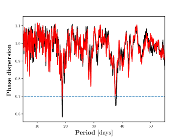
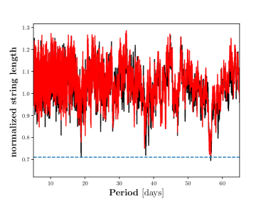
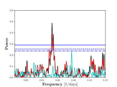
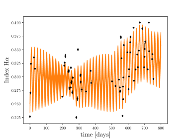
Figure 11: Results for BD+61 195 as explained in Fig. 10.

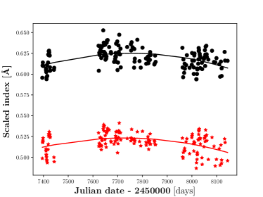
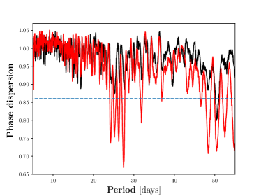
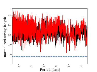
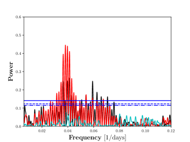
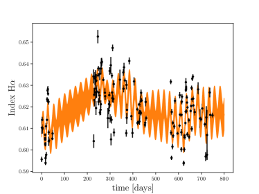
Figure 12: Results for BD+21 652 as explained in Fig. 10.

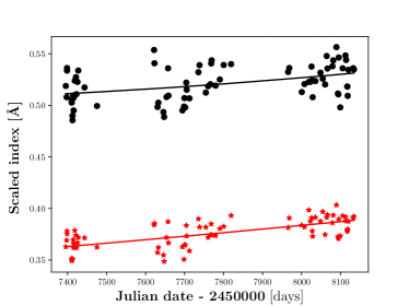
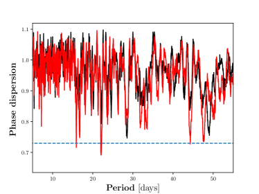
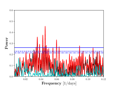
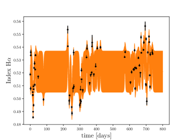
Figure 13: Results for BD+52 857 as explained in Fig. 10.

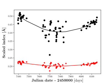
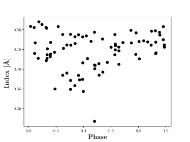
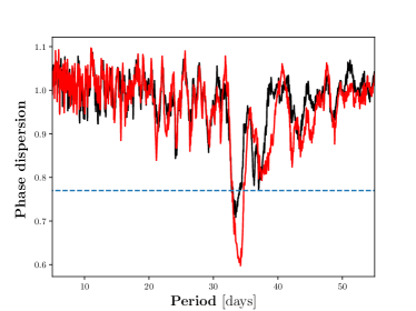
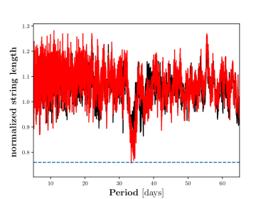
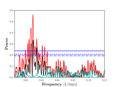
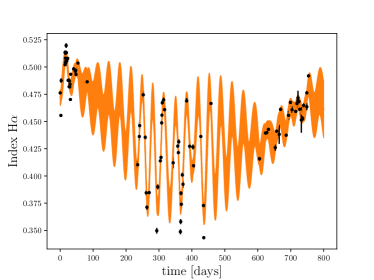
Figure 14: Results for HD 36395 as explained in Fig. 10.

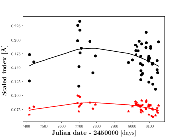
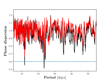
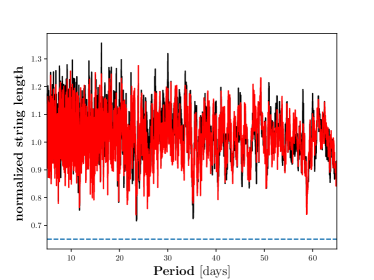
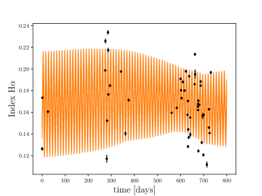
Figure 15: Results for V2689 Ori as explained in Fig. 10.

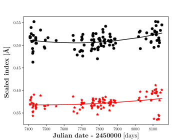
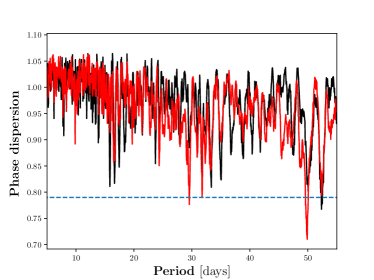
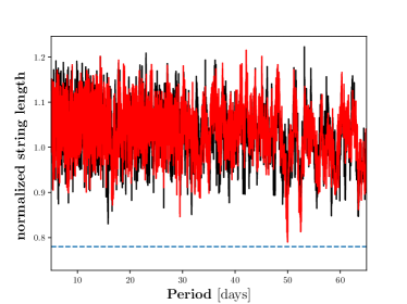
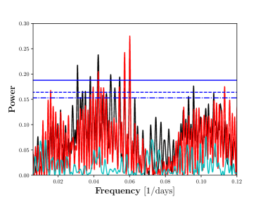
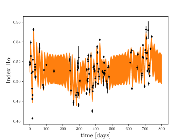
Figure 16: Results for HD 79211 as explained in Fig. 10.

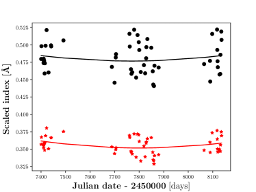
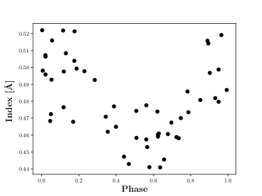
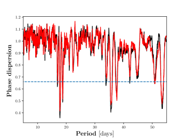
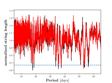
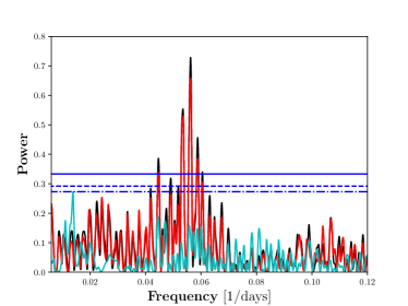
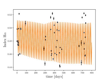
Figure 17: Results for BD+63 869 as explained in Fig. 10.

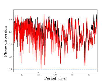
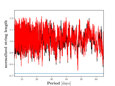
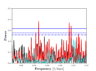
Figure 18: Results for AN Sex as explained in Fig. 10.

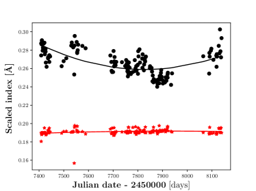
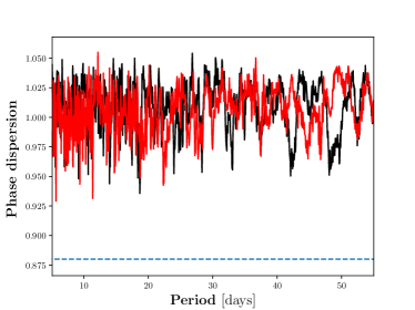
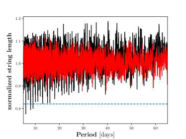
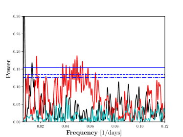
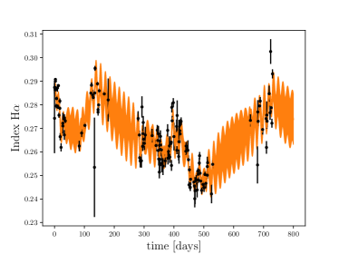
Figure 19: Results for Lalande 21185 as explained in Fig. 10.

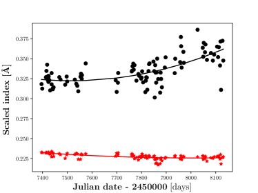
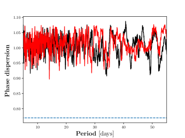
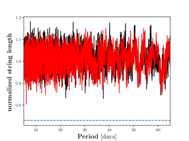
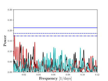
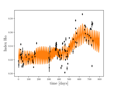
Figure 20: Results for BD+44 2051A as explained in Fig. 10.

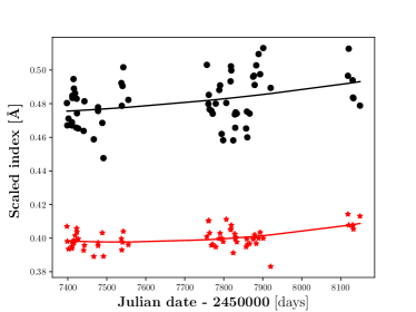
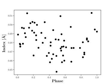
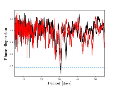
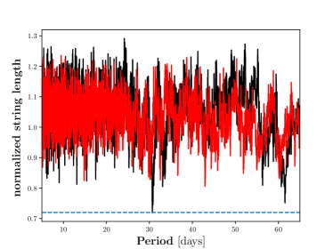
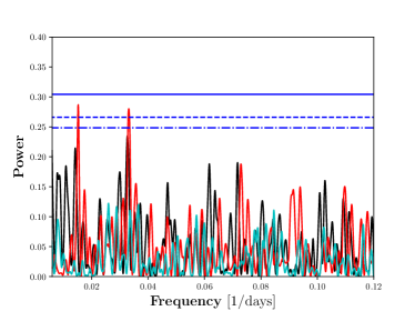
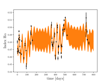
Figure 21: Results for BD+11 2576 as explained in Fig. 10.

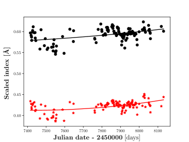
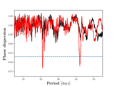
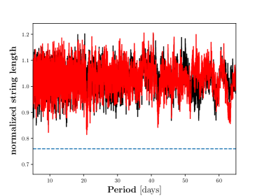
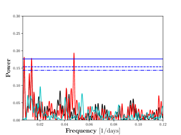
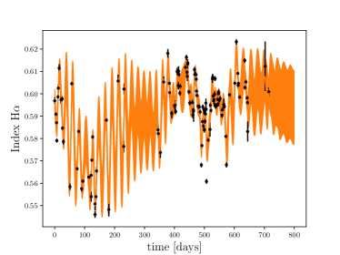
Figure 23: Results for HD 147379 as explained in Fig. 10.

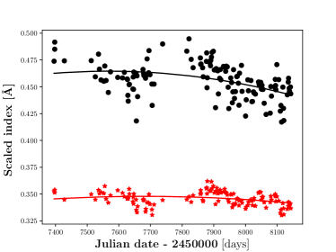
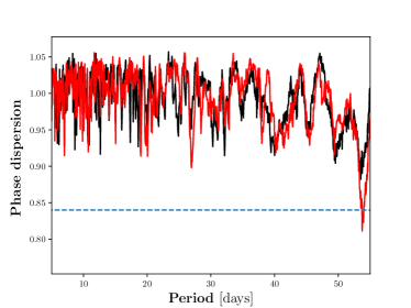
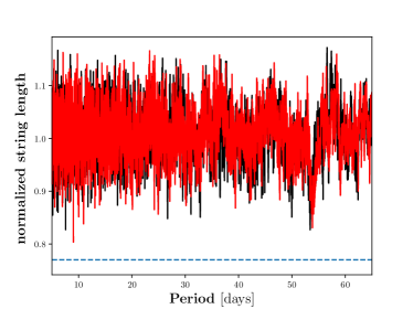
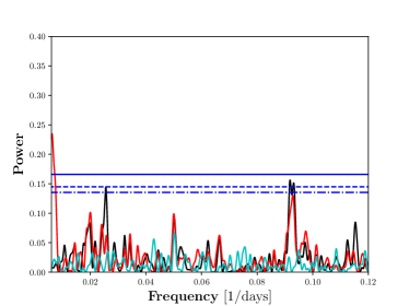
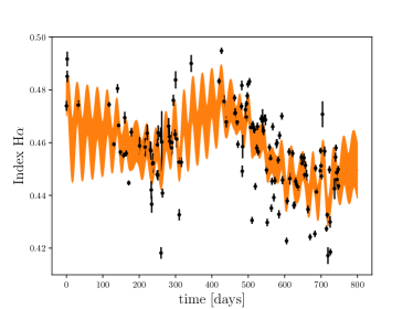
Figure 24: Results for HD 199305 as explained in Fig. 10.

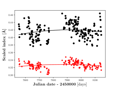
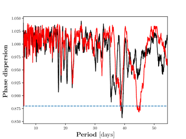
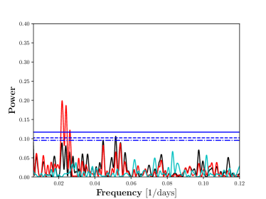
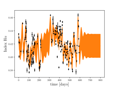
Figure 25: Results for HD 216899 as explained in Fig. 10.