Extended stream functions for dynamics of Bose-Einstein condensations:
Snake instability of dark soliton in ultra-cold atoms as an example

Abstract

In this paper, we formulate extended stream functions (ESFs) to describe the dynamics of Bose-Einstein condensations in the two-dimensional space. The ordinary stream function is applicable only for stationary and incompressible superfluids, whereas the ESFs can describe the dynamics of compressible and non-stationary superfluids. The ESFs are composed of two stream functions, i.e., one describes the compressible density modulations and the other the incompressible rotational superflow. As an application, we study the snake instability of the dark soliton in a rectangular potential in detail by the ESFs.

I Introduction

In the past decade, ultracold atomic systems are one of the most actively studied fields in physics. It is expected that these systems can be a quantum simulator for various models in quantum physics qsimu . Another aim to study ultracold atoms is to search for new quantum phenomena whose existence is theoretically predicted. These example are the supersolid that has both a diagonal solid order and an off-diagonal superfluid order SS , bosonic analog of fractional quantum Hall effect FQHE , etc. Because of their versatility and controllability, atomic gas systems are used for study on dynamics of Bose-Einstein condensates (BEC), in particular, formation and destruction of topological excitations such as vortices. Detailed study on such dynamical process was given in Refs. vortex1 ; vortex2 ; vortex3 ; vortex4 , and it shed a light on the dynamics of vortices, which is a long standing problem since the late 19th hydro .

In this paper, we focus on two-dimensional (2D) BEC and superfluidity (SF). Recently, vortex dynamics in annular and cylindrical BEC was studied by using stream function of the SF stF1 ; stF2 . In these systems, incompressible and irrotational stationary states of the SF can be analytically studied by the stream function. In order to extend the stream-function formalism to compressible, irrotational and non-stationary fluid, a pair of stream functions are needed. That is, one describes rotational flow, and the other compressible component of flow. We call them extended stream functions (ESFs) in this paper. As we show in the rest of this paper, the ESFs, in our definition, are numerically obtained without any difficulties and they are quite useful for detailed study on SF dynamics.

The present paper is organized as follows. In Sec. II, we introduce the ESFs, and their relation to the Gross-Pitaevskii equation (GPE) is explained. In order to verify the reliability and accuracy of the practical manipulation to obtain the incompressible and irrotational components of SF flow from the ESFs, we apply our formalism for an annular SF. By a sudden quench of an synthetic magnetic field, a homogeneous BEC becomes unstable, and vortex formation takes place. We describe this evolution of the BEC by the ESFs and compare the results with those obtained directly from the solution to the GPE. In Sec. III, we apply the ESFs formalism for certain typical phenomenon of the SF instability. As an example, we study the time evolution of a dark soliton DS1 ; DS2 ; DS3 located in the center of a rectangular potential BV . This dark soliton exhibits a snake instability and the central empty region changes its shape, and vortices and antivortices are generated there. We show that the ESFs clearly describe this process of the destruction of the dark soliton and formation of vortex-antivortex chain. Section IV is devoted for conclusion.

II Extended stream functions

As we explained in introduction, we mostly study the BEC in the ultra-cold bosonic atoms by solving the GPE,

$$(i-\gamma){\partial\psi\over\partial t} = -{1\over 2}\nabla^{2}\psi+V(r)\psi+g|\psi|^{2}\psi$$ (1)

$$-\bar{\mu}\psi-\omega L_{z}\psi,$$

where $\gamma$ is a phenomenological dissipation parameter, $V(r)$ is potential, $g$ is the coupling constant for the repulsion, and $\bar{\mu}$ is the chemical potential. We have put the atomic mass $m=1$, and also the Planck constant is set $\hbar=1$. For example, the unit of time $t=1$ corresponds to $7.94$ ms for ⁸⁷Rb confined by the 2D harmonic trap with $\omega_{\bot}=20.1\times 2\pi$ Hz vortex4 . We use this energy scale and the unit of time as well as the normalization, such as $\int dxdy|\psi|^{2}=1$, in the rest of present study. For the system under a rotation, $\omega$ is the angular velocity of the rotation and $L_{z}$ is the angular momentum in the $z$-direction. We are in the co-moving frame of the atoms in Eq. (1). In the rest of this work, we solve the GPE in Eq. (1) for specific $V(r)$, initial conditions, etc, and study the dynamics of the BEC in detail. To this end, we introduce the ESFs. The ESFs are applicable for various physical systems with flow. In this paper, we use them for study on SF of ultra-cold atoms.

In the previous works using the ordinary stream function, incompressible and stationary BEC is considered stF1 ; stF2 . For compressible and non-stationary flows of SF, the continuity equation is given as follows,

$${\partial\rho\over\partial t}+\nabla\cdot(\rho\vec{v})=0,$$ (2)

where $\rho\equiv|\psi|^{2}$ and $\vec{v}\equiv{1\over 2i\rho}(\psi^{\ast}\nabla\psi-\psi\nabla\psi^{\ast})=\nabla\theta$ with $\psi=|\psi|e^{i\theta}$. For incompressible and stationary BEC, the continuity equation, Eq. (2), reduces $\nabla\cdot\vec{v}=0$. Therefore in 2D systems, the velocity $\vec{v}$ can be expressed as follows by using a function $\chi(\vec{r})$, which is called stream function,

$$v_{x}=-{\partial\chi\over\partial y},\;\;v_{y}={\partial\chi\over\partial x},$$ (3)

where $\vec{r}=(x,y)$. On the other hand by the velocity potential $\Phi(\vec{r})$, the velocity $\vec{v}$ is expressed as

$$v_{x}={\partial\Phi\over\partial x},\;\;v_{y}={\partial\Phi\over\partial y}.$$ (4)

Then, it is useful to introduce the complex potential such as $F(z)\equiv\chi(z)+i\Phi(z)$, where $z$ is the complex coordinate $z=x+iy$. From Eqs. (3) and (4), it is obvious that $F(z)$ satisfies the Cauchy-Riemann condition. As a result, problems with various boundary conditions can be connected by a conformal mapping.

In this work, we generalize the above stream function in order to study the compressible and non-stationary quantum flows, $\vec{j}={1\over 2i}(\psi^{\ast}\nabla\psi-\psi\nabla\psi^{\ast})$. To this end, we introduce a pair of stream functions, $\tilde{\chi}(\vec{r},t)$ and $\tilde{\Phi}(\vec{r},t)$, the ESFs. The flow $\vec{j}$ is composed of the incompressible and irrotational (compressible) parts, i.e.,

$$\vec{j}=\rho\nabla\theta=(\rho\nabla\theta)_{i}+(\rho\nabla\theta)_{c}\equiv\vec{j}_{i}+\vec{j}_{c},$$ (5)

where $(\rho\nabla\theta)_{i}$ and $(\rho\nabla\theta)_{c}$ stand for the incompressible and irrotational components of the flow, respectively. Each of the above components is repressed by the ESFs as follows,

$$(\rho\nabla\theta)_{i}=\hat{z}\times\nabla\tilde{\chi},\;\;(\rho\nabla\theta)_{c}=\nabla\tilde{\Phi},$$ (6)

where $\hat{z}$ is the unite vector in the $z$-direction. The following equalities are easily verified,

$$\nabla\times\vec{j}=\Delta\tilde{\chi},\;\;\nabla\cdot\vec{j}=\Delta\tilde{\Phi}.$$ (7)

The continuity equation (2) is expressed as,

$${\partial\rho\over\partial t}+\Delta\tilde{\Phi}=0.$$ (8)

It should be remarked here that the ESFs $\tilde{\chi}$ and $\tilde{\Phi}$ include the density $\rho$ in their definition, and therefore they are well defined for configurations including vortices. Furthermore for the system confined by a trap potential $V(r)$, the BEC has boundaries at which the density vanishes. This means that no boundary conditions are needed to obtain $\tilde{\chi}$ and $\tilde{\Phi}$ as we see later on.

From the definition Eq. (6), typical profiles of $\tilde{\chi}$ and $\tilde{\Phi}$ that correspond the flows $j_{i}$ and $j_{c}$ as shown in Fig. 1. These profiles are useful to understand what the numerical calculations of $\tilde{\chi}$ and $\tilde{\Phi}$ indicate in the later discussion.

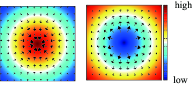
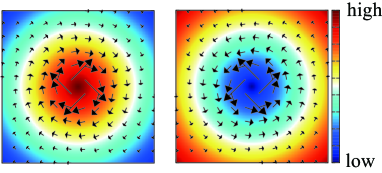
Figure 1: Typical profiles of the ESFs, and compressible and incompressible flows of the BEC. $\tilde{\Phi}$ in upper panels (the compressible component), and $\tilde{\chi}$ (the rotational incompressible component) in lower panels. Arrows indicate flow of each component.

As we show in the rest of the present paper, the ESFs describe detailed behavior of the BEC in a transparent way. In the practical calculation, we obtain $\tilde{\chi}$ and $\tilde{\Phi}$ from the current $\vec{j}(x,y,t)=\vec{j}(\vec{r},t)$ by using the Fourier/inverse-Fourier transformations,

$$\tilde{\chi} = -F^{-1}\Big{[}{1\over k^{2}_{x}+k^{2}_{y}}F[\nabla\times\vec{j}]\Big{]},$$

$$\tilde{\Phi} = -F^{-1}\Big{[}{1\over k^{2}_{x}+k^{2}_{y}}F[\nabla\cdot\vec{j}]\Big{]},$$ (9)

where $F$ and $F^{-1}$ denote the operator of the Fourier and inverse-Fourier transformations, respectively.

In order to verify the utility of the ESFs and reliability of the numerical manipulations of the present formalism, we studied the sudden quench dynamics of BEC confined in a 2D torus, which was studied in the previous works. Abrupt application of an artificial magnetic field renders homogeneous BEC unstable. To see how the BEC evolves in the process, we solve the GPE in Eq. (1). For the numerical calculation, we used the following parameters; $\gamma=0.03$, $V(r)=30(r-4)^{2}$, $g=1000$, $\omega=0\to 1.9$, and the time and spatial meshes for the calculation are $dx,dy=0.05$ and $dt=0.005$, respectively.

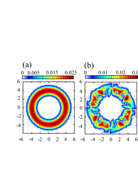
Figure 2: (a) Evolution of BEC density $\rho$ in a torus after the sudden quench of the external magnetic field. ($t=10$.) (b) Surface ripples propagating the along the surface appear. ($t=14$.) (c) Stable vortex lattice forms. ($t=100$.)

Evolution of the SF is as follows vortex4 . First, surface ripples propagating along the surface appear and then, they gradually develop into vortex cores, and finally vortices enter into the BEC and a vortex lattice forms. See Fig. 2. We compared the current $\vec{j}(\vec{r},t)$ obtained directly from the numerical solutions of the GPE and that obtained through the ESFs, $\tilde{\chi}(\vec{r},t)$ and $\tilde{\Phi}(\vec{r},t)$, in the final stage (the stage (c) in Fig. 2), and found that these two calculations are in good agreement.

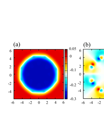
Figure 3: ESFs (a) $\tilde{\chi}$ and (b) $\tilde{\Phi}$ in the final stage of the BEC evolution after the sudden quench (the stage (c) in Fig. 2). The incompressible component flow described by $\tilde{\chi}$ circulates around the torus. On the other hand, the compressible component $\tilde{\Phi}$ has a pair of source and drain corresponding to each vortex.

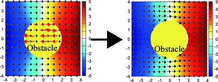
Figure 4: ESFs in the vicinity of an obstacle such as a vortex. The incompressible component described by $\tilde{\chi}$ is not influenced by the obstacle, whereas the compressible component $\tilde{\Phi}$ generates counter-flow to cancel the $\tilde{\chi}$-flow inside of the obstacle.

It is quite instructive to see how the ESFs describe the process of vortex lattice formation in the above quench dynamics. In Fig. 3, we first show the ESFs $\tilde{\chi}(\vec{r})$ and $\tilde{\Phi}(\vec{r})$ for the vortex lattice BEC that formed at the final stage of the evolution. Profile of $\tilde{\chi}(\vec{r})$ shows that $\tilde{\chi}(\vec{r})$ is a smooth function and a steady counter-clockwise SF flow exists inside of the torus. Behavior of $\tilde{\chi}(\vec{r})$ is not influenced substantially by the existence of the vortices as it describes the incompressible (rotational) component of the SF flow. On the other hand, $\tilde{\Phi}(\vec{r})$ exhibits an interesting profile. High and low-$\tilde{\Phi}$ regions always appear in a pair, and we call this configuration dimer. Around the locations of vortex, a pair of dimer forms, and in the regions between dimers $\tilde{\Phi}\sim 0$. Schematic picture of this $\tilde{\Phi}$ configuration in the vicinity of an obstacle (e.g., vortex) is shown in Fig. 4. It shows that the compressible component $\vec{j}_{c}$ cancels the flow of the incompressible component $\vec{j}_{i}$ inside of the obstacle. As a result, the SF density inside of the obstacle is kept vanishing as $\rho\nabla\theta=\vec{j}=\vec{j}_{c}+\vec{j}_{i}\simeq 0$.

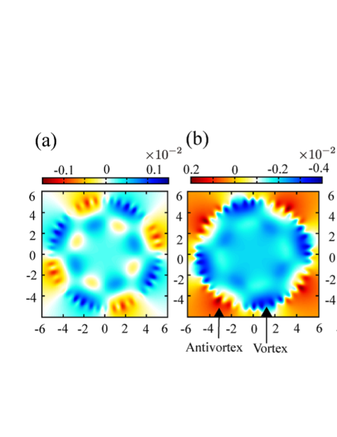
Figure 5: ESF $\tilde{\chi}$ in the process after the quench. (a) Surface ripples propagating along the surface appear first. ($t=10$.) (b) Vortex and antivortex are generated in a pair inside the torus. ($t=11$.) (c) Only vortices remain in the torus. SF flows are circulating in the surface of the torus. ($t=12$.)

Finally, we see how the BEC develops towards the stable state in Fig. 2 by the stream function $\tilde{\chi}(\vec{r},t)$. First, surface instability after the sudden quench generates vortex and antivortex in the both sides of the boundary as show in Fig. 5. Then, the calculations of $\tilde{\chi}(\vec{r},t)$ show that vortices move into the BEC whereas antivortices leave for the outside of the BEC. The incompressible current $\vec{j}_{i}$ flows counter-clock wise in the BEC via the effect of the synthesized magnetic field.

In the following section, we shall study the instability of the dark soliton and formation of snake soliton by using the ESFs.

III Extended stream functions and snake instability of dark soliton

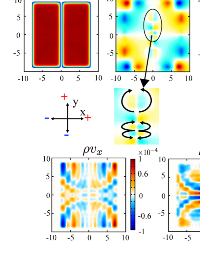
Figure 6: BEC density $\rho$, ESFs $\tilde{\chi}$ and $\tilde{\Phi}$, and velocity in the first stage of the destruction process of the dark soliton located at the center of the potential. ($t=3.0$.) The arrows indicate the incompressible and compressible components of the SF velocity. The velocity exhibits strong dependence of the $y$-coordinate, and it induces a primordial movement of the snake instability to the second stage.

In this section, as an example of the dynamical behavior of BEC described by the ESFs, we study the instability of a dark soliton located in the center of a rectangular confinement potential. In GPE in Eq. (1), we put $\omega=0$ and

$$V(x,y)=\left\{\begin{array}[]{ccr}0,&(|x|<8,|y|<9)\\ 100,&(\mbox{otherwise}).\end{array}\right.$$ (12)

The initial configuration at $t=0$ is produced by imprinting the dark soliton profile on the homogeneous BEC state such as $\psi_{0}(x)=n_{0}\tanh(\mu x)$ with constants $n_{0}$ and $\mu$ DSWF . We study how this dark soliton evolves by the ESFs.

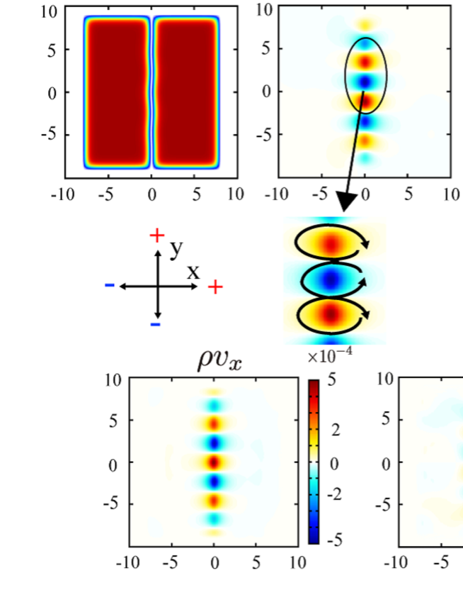
Figure 7: BEC density $\rho$, ESFs $\tilde{\chi}$ and $\tilde{\Phi}$, and velocity in the second stage of the destruction process of the dark soliton located at the center of the potential. ($t=20.1$.) The arrows indicate the incompressible and compressible components of the SF velocity. The velocity exhibits a strong dependence of the $y$-coordinate.

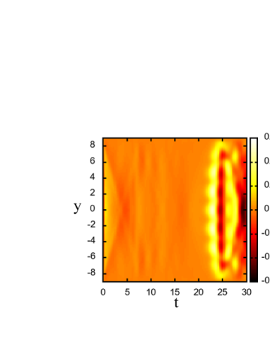
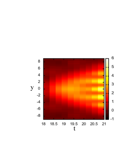
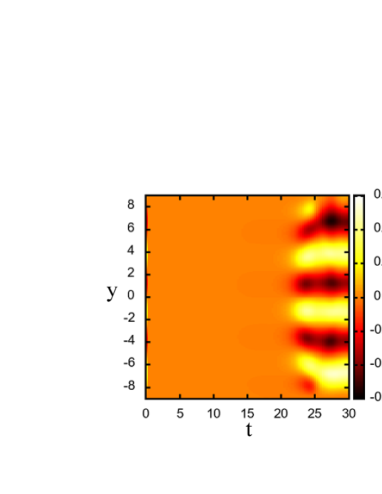
Figure 8: Upper panels: BEC flow $Q(y,t)$ in Eq. (19) that measures amount of SF-density flow from $y=-9$ to $y$. Lower panels: BEC flow through the $x=0$ line, $R(y,t)$, in Eq. (20) that measures amount of the incompressible SF flow from $y=-9$ to $y$. The both results indicate the snake instability to the stage 2.

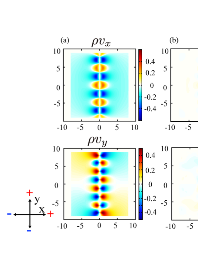
Figure 9: Vortex-antivortex configurations. (a) The flow profiles obtained by the analytical expression in Eq. (21). (b) That obtained by the numerical simulation in the process of the snake instability of the dark soliton. These two are rather similar, but the configuration (b) has nontrivial flows only in the central region. This comes from the fact that the configuration (b) forms in the process of the dark soliton instability.

The continuity equation is given as follows,

$${\partial(\rho_{0}(\vec{r})+\delta\rho(\vec{r},t))\over\partial t} = {\partial\delta\rho(\vec{r},t)\over\partial t}$$

$$= -\nabla\cdot\vec{j}(\vec{r},t)$$

$$= -\nabla\cdot((\rho_{0}(\vec{r})+\delta\rho(\vec{r},t))\delta\vec{v}(\vec{r},t)),$$

where $\rho_{0}(\vec{r})=\psi^{2}_{0}(x)$. On the other hand by using the ESFs,

$$(\rho_{0}(\vec{r})+\delta\rho(\vec{r},t))\delta\vec{v}(\vec{r},t)=\nabla\tilde{\Phi}+\hat{z}\times\nabla\tilde{\chi}.$$ (14)

By substituting $\rho_{0}(\vec{r})=\psi^{2}_{0}(x)$ into Eq. (14) and ignoring term such as $\nabla\delta\rho\times\delta\vec{v}$, we obtain

$$\Delta\tilde{\chi}(\vec{r},t) = 2n_{0}^{2}\mu{\tanh(\mu x)\over\cosh^{2}(\mu x)}\delta v_{y}(\vec{r},t)$$ (15)

$$+(\rho_{0}(\vec{r})+\delta\rho(\vec{r},t))\nabla\times\delta\vec{v}.$$

In the second term on the RHS of Eq. (15), for a configuration of vortex at $\vec{r}=\vec{r}_{0}$, $\nabla\times\delta\vec{v}\propto\delta(\vec{r}_{0})$. However in this case, $(\rho_{0}(\vec{r}_{0})+\delta\rho(\vec{r}_{0},t))\simeq 0$, and therefore this term is negligibly small. Similarly for $\tilde{\Phi}(\vec{r},t)$,

$$\Delta\tilde{\Phi}(\vec{r},t) = 2\mu n_{0}^{2}{\tanh(\mu x)\over\cosh^{2}(\mu x)}\delta v_{x}(\vec{r},t)$$

$$+n_{0}^{2}\tanh^{2}(\mu x)\nabla\cdot\delta\vec{v}(\vec{r},t)+\delta\rho\nabla\cdot\delta\vec{v}(\vec{r},t).$$

For the first stage of the evolution with $t\ll 1$, the numerical calculations of $\rho(\vec{r},t)$, $\tilde{\chi}(\vec{r},t)$ and $\tilde{\Phi}(\vec{r},t)$, etc. by using Eq. (9) are shown in Fig. 6. The BEC is approximately symmetric under $x\to-x$,

$$\delta\rho(x,y,t)\simeq\delta\rho(-x,y,t),$$

$$\delta v_{x}(x,y,t)\simeq-\delta v_{x}(-x,y,t),$$ (17)

$$\delta v_{y}(x,y,t)\simeq\delta v_{y}(-x,y,t).$$ (18)

In this case, $\tilde{\chi}(\vec{r},t)$ is anti-symmetric under $x\to-x$, as observed by the numerical calculation in Fig 6. Furthermore, the numerical calculations in Fig. 6 show that $\delta v_{y}$ in the region $x\sim 0$ has strong $y$ dependence as the both compressive and incompressible components do. On the other hand on the line $x=0$, $\delta v_{x}=0$, whereas ${\partial\delta v_{x}\over\partial x}\neq 0$ by the incompressible component, and therefore the second term on the RHS of Eq. (III) contributes to $\Delta\tilde{\Phi}(\vec{r},t)$ in the small but finite $x$ region. The relatively large $\nabla\cdot\delta\vec{v}$ induces a density modulation $\delta\rho$ through Eq. (III) and the continuity equation Eq. (8). This is a primordial movement of the snake instability.

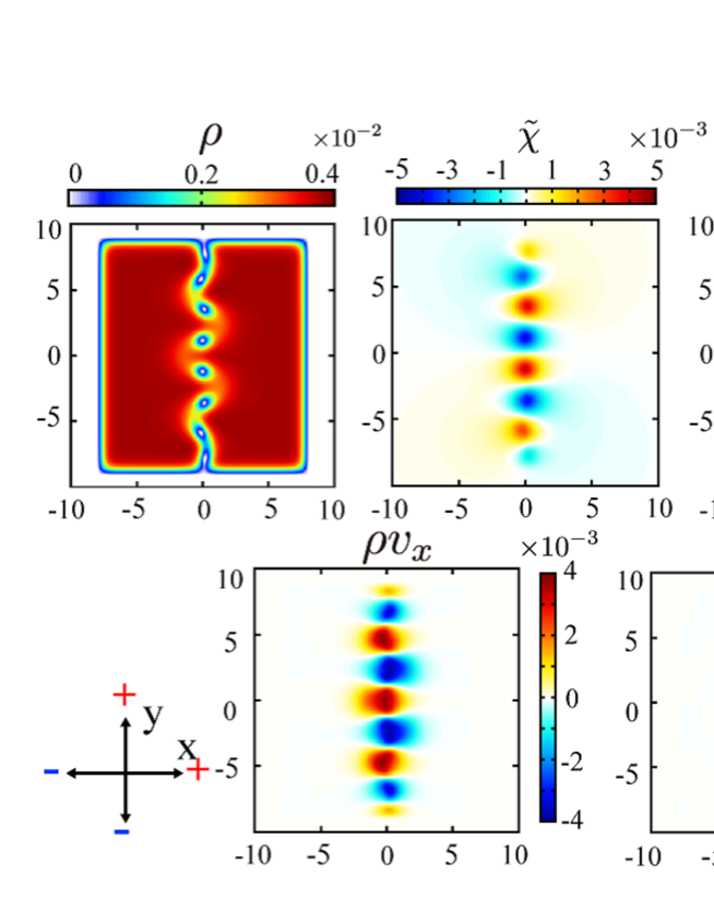
Figure 10: BEC density $\rho$, ESFs $\tilde{\chi}$ and $\tilde{\Phi}$, and velocity in the third stage of the destruction process of the dark soliton located at the center of the potential. ($t=23.4$.) The velocity exhibits a strong dependence of the $y$-coordinate.

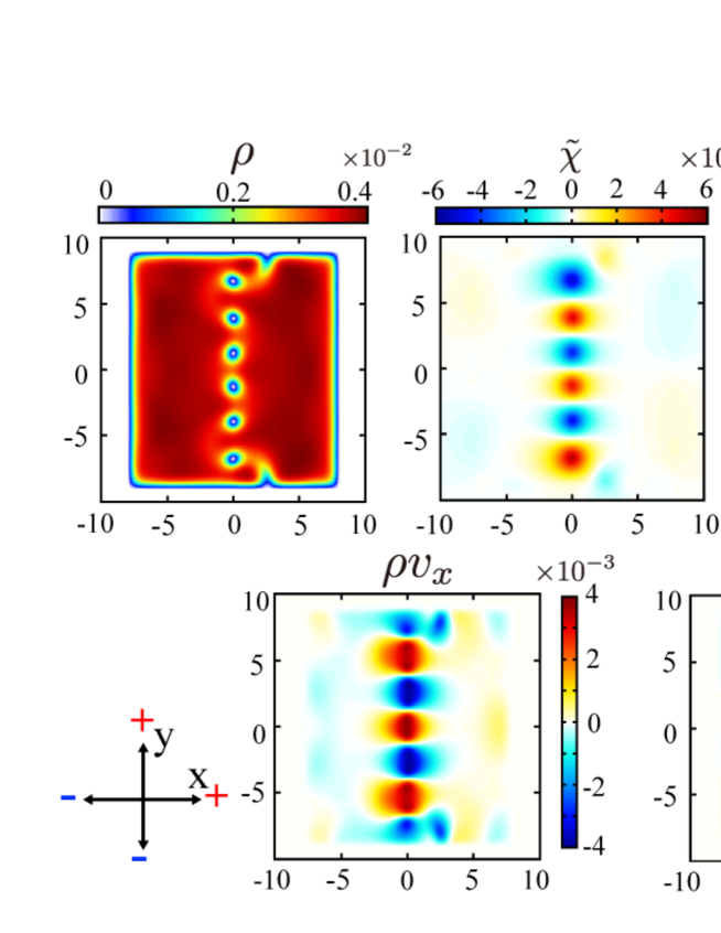
Figure 11: BEC density $\rho$, ESFs $\tilde{\chi}$ and $\tilde{\Phi}$, and velocity in the fourth stage of the destruction process of the dark soliton located at the center of the potential. ($t=27.0$.) Isolated vortex droplets form and this fourth stage is stable against the pair annihilation of vortex and antivortex.

In the second stage of the evolution, the numerical results of the ESFs in Fig. 7 reveal that $\delta v_{x}$ comes from both the compressible and incompressible flows, whereas $\delta v_{y}$ from the compressible component. As $\tilde{\Phi}$ in Fig. 7 shows, the central empty line slightly deforms to a meandering line by the density flow explained above.

By the numerical simulation, we observed that the second stage is a meta-stable state. It is interesting to see how it forms from the BEC in the first stage. In Fig. 8, we show the incompressible SF density flow at $t$, $Q(y,t)$, defined by

$$Q(y,t) = \int^{y}_{y_{0}}\rho(0,y^{\prime},t)\vec{v}(0,y^{\prime},t)\cdot\hat{y}dy^{\prime}$$ (19)

$$= \tilde{\Phi}(0,y,t)-\tilde{\Phi}(0,y_{0},t),$$

where $\hat{y}$ in the unit vector in the $y$-direction, and we put $y_{0}=-9$. From the calculations in Fig. 8, it is seen that a density modulation starts to form at the center of the dark soliton ($y\simeq 0$) at $t\sim 18$ and then it spreads in the $y$-direction. Similarly, we show the SF incompressible flow in Fig. 8, $R(y,t)$, which is defined as

$$R(y,t) = \int^{y}_{y_{0}}\rho(0,y^{\prime},t)\vec{v}(0,y^{\prime},t)\cdot\hat{x}dy^{\prime}$$ (20)

$$= \tilde{\chi}(0,y,t)-\tilde{\chi}(0,y_{0},t).$$

$R(y,t)$ shows that the snake instability is enhanced by the incompressible SF flow as well as the incompressible flow.

It is also interesting to see how the vortices and antivortices form in the central-meandering low-density region in the second stage. To observation this, we calculate the SF current generated by vortices and antivortices by employing analytic functions as a reference. For example, the flow in a typical vortex-antivortex configuration is given as,

$$\rho v_{x}=\tanh^{2}(\mu x)\Big{(}\sum_{i=1}^{8}{-s_{i}(y-y_{i})\over x^{2}+(y-y_{i})^{2}}\Big{)},$$

$$\rho v_{y}=\tanh^{2}(\mu x)\Big{(}\sum_{i=1}^{8}{s_{i}(x-x_{i})\over x^{2}+(y-y_{i})^{2}}\Big{)}$$ (21)

where the vortices and antivortices are located alternatively at $(x_{i},y_{i})$ with $x_{i}=0$ and $y_{i}=8,6,3.6,1.25,-1.25,-3.6,-6$ and $-8$, and the vorticity $s_{i}$ is given by $s_{i}=(-)^{i}$. Configuration of the above flow (21) is shown in Fig. 9, which exhibits a qualitative similar profile to that in Fig. 7 in the central region, but the configuration given by Eq. (21) has a nontrivial flows in the wider region compared to the results in Fig. 7. This difference comes from the fact that vortex configuration in Fig. 7 have just formed in the second stage, and therefore the region far apart from the central region is not influenced by the vortex formation.

The density flow in Fig. 7 continues after the second stage, and then the empty line in the central region of the SF splits into smaller lines and droplets. This is the third stage in Fig. 10. This behavior continues to the fourth stage in Fig. 11, in which a line of droplets form. Each droplet corresponds to vortex or antivortex as the ESF, $\tilde{\chi}(\vec{r},t)$, indicates. That is, vortices and antivortices align in a straight line alternatively. We observed that this fourth stage is rather long-lived, even though a pair annihilation of vortex and antivortex is possible.

IV Conclusion

In this work, we introduced the ESFs to describe dynamics of non-stationary and compressible SF. To this end, two components of the ESFs, $\tilde{\chi}$ and $\tilde{\Phi}$, are necessary. By the definition of the ESFs, vortices can be described with regular $\tilde{\chi}$ and $\tilde{\Phi}$, and also specific boundary conditions are not necessary in the confinement potential problems. We showed the numerical methods to obtain the ESFs, and applied the ESFs to the sudden quench of SF in the torus by applying a synthetic magnetic field. We found good agreement between the results obtained by our methods and those by the direct calculations from the solutions to the GP equation.

Then, we applied our methods to detailed study on the snake instability of the dark soliton in the rectangular potential. We found that there exist four typical stages in the process, and clarified dynamics of the SF flow in the whole process of the instability towards the meta-stable state with vortex droplets.

We hope that the ESFs given in the present work are useful for study on various dynamics of SF. This problem is under study, and we hope that results will be reported in the near future.

References

- (1) M. Lewenstein, A. Sanpera, and V. Ahufinger, Ultracold Atoms in Optical Lattices: Simulating Quantum Many-body Systems (Oxford University Press, 2012).
- (2) G. G. Batrouni, R. T. Scalettar, G. T. Zimanyi,and A. P. Kampf, Phys. Rev. Lett. 74, 2527 (1995); K. Góral, L.Santos, and M. Lewenstein, Phsy. Rev. Lett. 88, 170406 (2002); V. W. Scarola and S. Das Sarma, Phys. Rev. Lett. 95, 033003 (2005); C. Menotti, C. Trefzger, and M. Lewenstein, Phys.Rev. Lett. 98, 235301 (2007); K.-K. Ng and Y.-C. Chen, Phys.Rev. B. 77, 052506 (2008); I. Danshita and C.A.R. Sa de Melo, Phys. Rev. Lett. 103, 225301 (2009); B. Capogrosso-Sansone, C. Trefzger, M. Lewenstein, P. Zoller, and G. Pupillo, Phys. Rev. Lett. 104, 125301 (2010); K.-K. Ng, Phys.Rev. B. 82, 184505 (2010); H. Ozawa and I. Ichinose, Phys.Rev. A. 86, 015601 (2012).
- (3) A. Sorensen, E. Demler and M. Lukin, Phys. Rev. Lett.94.086803 (2005); M. Hafezi, A. Sorensen, E. Demler and M. Lukin, Phys. Rev. A 76, 023613 (2007); M. O. Oktel, M. Nita, and B. Tanatar, Phys. Rev. B 75, 045133 (2007); R. O. UmucalIlar and E. J. Mueller, Phys. Rev. A 81, 053628 (2010); Y. Kuno, K. Shimizu, and I. Ichinose, Phys. Rev. A 95, 013607 (2017); R. Bai, S. Bandyopadhyay, S. Pal, K. Suthar, and D. Angom Phys. Rev. A 98 023606 (2018).
- (4) S. Sinha and Y. Castin, Phys. Rev. Lett. 87, 190402 (2001).
- (5) M. Tsubota, K. Kasamatsu, and M. Ueda, Phys. Rev. A 65, 023603 (2002); K.Kasamatsu, M. Tsubota, and M. Ueda, ibid. 67, 033610 (2003).
- (6) N. G. Parker, R. M. W. van Bijnen, and A. M. Martin, Phys. Rev. A 73, 061603(R) (2006).
- (7) A. Kato, Y. Nakano, K. Kasamatsu, and T. Matsui, Phys. Rev. A 84, 053623 (2011).
- (8) H. Lamb, Hydrodynamics, 6th. ed. (Dover Publication, New York, 1945).
- (9) L.A. Toikka and K.-A. Suominen, Phys. Rev. A 93, 053613 (2016).
- (10) N.-E. Guenther, P. Massignan, and A. L. Fetter, Phys. Rev. A 96, 063608 (2017).
- (11) P. G. Kevrekidis, D. J. Frantzeskakis, and R. Carretero-González, Emergent Nonlinear Phenomena in Bose-Einstein Condensates (Springer, New York, 2008).
- (12) D. J. Frantzeskakis, J. Phys. A: Math. Theor. 43, 213001 (2010).
- (13) P. G. Kevrekidis, D. J. Frantzeskakis, and R. Carretero-González, The Defocusing Nonlinear Schrëdinger Equation (Society for Industrial and Applied Mathematics, Philadelphia, PA, 2015).
- (14) A. L. Gaunt, T. F. Schmidutz, I. Gotliborych, R. P. Smith, and Z. Hadzibabic, Phys. Rev. Lett. —bf 110, 200406 (2013).
- (15) G. Verma, U. D. Rapol, and R. Nath, Phys. Rev. A 95, 043618 (2017).