Coarse-Grained Methods for Heterogeneous Vesicles with Phase-Separated Domains:
Elastic Mechanics of Shape Fluctuations, Plate Compression, and Channel Insertion.

We develop coarse-grained particle approaches for studying the elastic mechanics of vesicles with heterogeneous membranes having phase-separated domains. We perform simulations both of passive shape fluctuations and of active systems where vesicles are subjected to compression between two plates or subjected to insertion into narrow channels. Analysis methods are developed for mapping particle configurations to continuum fields with spherical harmonics representations. Heterogeneous vesicles are found to exhibit rich behaviors where the heterogeneity can amplify surface two-point correlations, reduce resistance during compression, and augment vesicle transport times in channels. The developed methods provide general approaches for characterizing the mechanics of coarse-grained heterogeneous systems taking into account the roles of thermal fluctuations, geometry, and phase separation.

1 Introduction

Biological membranes consist of complex heterogeneous mixtures of different lipid species, proteins, and other small molecules [1, 2, 3]. Membrane heterogeneity is important to organize cellular structures and mechanical responses [4, 5, 6, 7, 8]. This includes the insertion, assembly, and activation of membrane-proteins such as channels, receptors, or anchoring sites of the cytoskeleton [3, 9, 10, 11, 12]. Phase domains also play a role in the initiation of the formation of buds and endocytosis [13, 14, 15, 16, 17], and in the local control of diffusivity [18, 19, 20, 8], fluidity [4], or bending moduli [15, 21, 7]. For applications and as model physical systems, synthetic soft membranes also have been introduced consisting of self-assembled particles with phases that can form sheets and other structures  [22, 23, 24, 25].

Heterogeneous membranes can exhibit rich behaviors and geometries arising from the phase-separated domains [15, 5, 26]. For spherical vesicles, phase separation kinetics and surface transport have been studied experimentally in [15, 5, 27]. To better understand the mechanics of heterogeneous membranes, we develop coarse-grained simulation approaches and analysis methods. We consider the case of vesicles with phase-separated domains having different preferred curvatures. Simulations are performed to study the impact of heterogeneity both on passive shape fluctuations and on vesicles subjected to active deformations. To characterize mechanical responses, analysis methods are developed for mapping particle configurations to continuum surface representations. Lebedev sampling and spherical harmonic expansions are used to develop spectral analysis methods for studying passive shape fluctuations and other geometric changes.

To investigate active deformations, simulation and analysis methods are developed for vesicles subjected to compression between two plates and subjected to insertion into narrow channels. We find heterogeneous vesicles can exhibit mechanical responses differing significantly from the homogeneous case. For heterogeneous vesicles, the phase domains are found to amplify surface two-point correlations. For vesicle compression, it is found that the phase-domains can rearrange to accommodate curvature in membrane bending to reduce energetic costs. In channel insertion and transport, the heterogeneity is found to have mixed effects depending on the circumstances which can either decrease or increase insertion and transport times.

There have been many continuum mechanics and coarse-grained methods developed for investigating multi-component membranes. At the continuum mechanics level, these include [28, 29, 30, 31, 32, 33, 34]. At the coarse-grained level, there are models of different levels of detail. Models incorporating some structure of the individual lipids include [35, 36, 37, 38, 39, 40] and implicit-solvent models [41, 42, 43, 44, 45, 36]. Models at a more coarse-grained level employing a single-bead to describe a cluster of lipids include [46, 47, 48, 49, 50]. Related models and methods for use in dynamic studies have been developed in [51, 52, 50, 53, 54]. In general, coarser models have the advantage of computationally facilitating access to larger length and time scales, but with the trade-off with the level of physical resolution at small scales [55, 56].

As a basis for our computational studies, we use the single-bead implicit-solvent coarse-grained model of Yuan et al. [47]. In this approach, the membrane is modeled by a collection of orientable beads having an additional director degree of freedom. For biological membranes, the beads can be thought of as representing small patches of lipids and their orientation as taking into account on a coarse-grained level the collective molecular-level orientation order within the patch. For synthetic colloidal membranes, the director-bead model can be interpreted as capturing the effective physical interactions of distinct colloidal particles that are orientable and with the sterics handled by spherical repulsive interactions. In our work, we use the molecular dynamics simulation framework referred to as Large-scale Atomic/Molecular Massively Parallel Simulator (LAMMPS) [57]. Related to [58] and our prior work [59], we develop stochastic time-step integration methods.

We also develop and implement custom analysis tools mapping particle configurations to continuum fields for characterizing behaviors of the models. The particle-based methods, combined with our analysis tools, yield approaches that can avoid some of the cumbersome aspects of continuum formulations, which often require formulations drawing on differential geometry and development of numerical discretizations [60, 53, 54]. In this way, we are able to handle similar geometric contributions and physical phenomena for the phase-separation and mechanics. Much of the modeling is then deferred to the particle-level resolution and parametrization. Our analysis tools provide general methods for relating such particle-based approaches to continuum-level concepts.

To quantitatively characterize our coarse-grained models and simulation results, we develop spectral analysis methods based on the continuum mappings. The vesicle shape is characterized using spherical harmonics expansions of the mapping operator constructed using Lebedev quadratures [61, 62, 63]. Results from statistical mechanics are used to analyze the passive shape fluctuations to estimate elastic bending moduli and other properties. This is studied when varying the vesicle size and phase concentrations.

In Section 2, the coarse-grained model and numerical methods are discussed. In Section 3, the simulation approaches are discussed. In Section 4, the spectral analysis methods are discussed. In Section 5, the results are discussed for the simulations of active deformations when vesicles are subjected to compressed between two plates or subjected to insertion into channels. The results show a few mechanisms by which phase-separated domains can impact the mechanical responses of heterogeneous vesicles relative to the homogeneous case. The developed approaches also can be used to study other experimental measurements and simulations for phenomena within heterogeneous membranes.

2 Coarse-Grained Approach

2.1 Single-Bead Coarse-Grained Model for Heterogeneous Membranes

We investigate the mechanics of heterogeneous vesicles at the level of coarse-grained models and continuum mechanics. As a mesoscopic description of the phase separation and mechanics, we utilize the single-bead coarse-grained model of Yuan et al. [47]. In this approach, the membrane is modeled by a collection of orientable spherical beads that have both a translational degree of freedom $\mathbf{r}_{i}$ for the center-of-mass location and a rotational degree of freedom $\mathbf{n}_{i}$ for the direction of orientation.

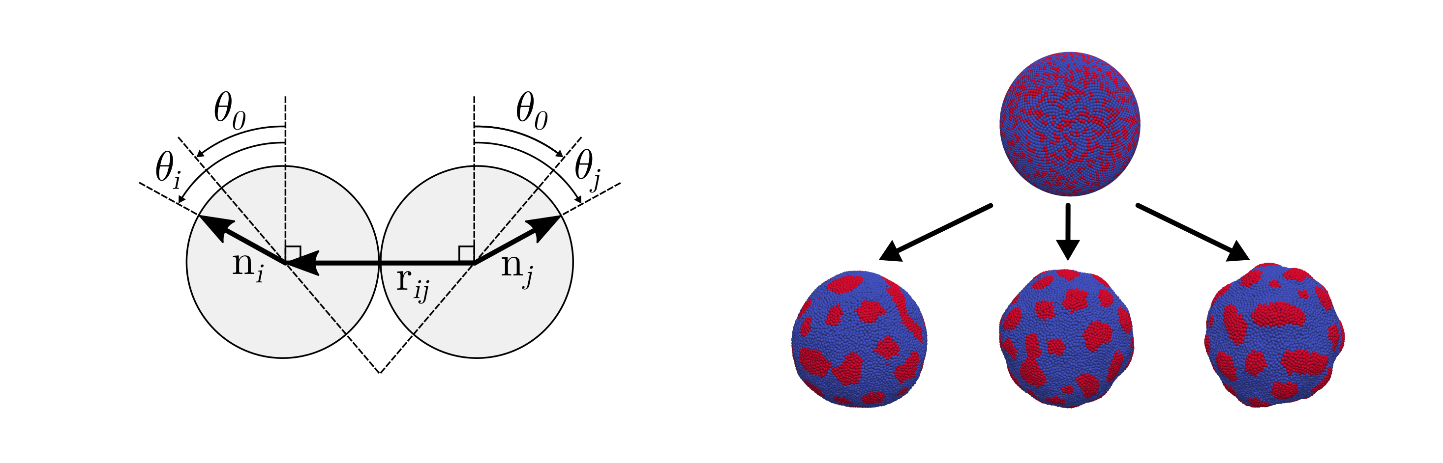
Figure 1: Coarse-grained particles and their interactions. The particles are at locations $\mathbf{r}_{i}$ and $\mathbf{r}_{j}$. The interactions depend on both the relative displacement $\mathbf{r}_{ij}$ and the orientations $\mathbf{n}_{i}$, $\mathbf{n}_{j}$. The $\theta_{i}$, $\theta_{j}$ give the in-plane angles. The interaction energy is given in equation (1), with minimization occurring when $|\mathbf{r}_{ij}|=\left(2\right)^{1/6}\sigma$ and $\theta_{i}=\theta_{j}=\theta_{0}$ (left). These interactions can have different affinities and preferred curvatures to drive phase-separation and shape changes in heterogeneous vesicles (right)

For lipid membranes, the beads can be thought of representing at the coarse-grained level a small patch of lipids with the orientation $\mathbf{n}_{i}$ serving as the local order parameter for the collective alignment of lipid molecules within the patch. This allows at the coarse-grained level to account for molecular interactions arising from hydrophilic-hydrophobic effects driving membrane assembly [64]. One could also interpret the model as a representation for a colloidal membrane with the beads representing individual colloidal particles having orientation-dependent interactions and spherical sterics. In either case, the orientation degrees of freedom $\mathbf{n}_{i}$ provide an important way to capture broken symmetries in the physical system that drive assembly of two-dimensional membrane sheets.

The parameters and quantities are referenced to the non-dimensional Lennard-Jones (LJ) characteristic scales $(\epsilon,\sigma,m)$. These are energy $\epsilon$, length $\sigma$, and mass $m$. We use characteristic time-scale $\tau\sim\sqrt{m\sigma^{2}/\epsilon}$. As in dimensional analysis, in this way our simulations reflect behaviors of all realizable physical systems in the equivalence class that are dynamically symmetric with respect to the characteristic LJ references. For instance, one can convert our results for the coarse-grained system to particular physical units by taking $\sigma$ to be the length-scale of a cluster of lipids, $m$ to be the mass of a cluster of lipids, and $\epsilon$ based on the temperature (thermal energy) of the system. To account for the interactions between two beads at location $\mathbf{r}_{i}$ and $\mathbf{r}_{j}$, unit vectors are introduced to account for the orientation $\mathbf{n}_{i}$ and $\mathbf{n}_{j}$. The relative displacement between the two beads is denoted by $\mathbf{r}_{ij}=\mathbf{r}_{i}-\mathbf{r}_{j}$. In these interactions, the beads have a preferred angle of alignment, which we denote by $\theta_{0}$. The interaction energy is minimized when $\theta_{i}=\theta_{j}=\theta_{0}$. The interactions between beads is illustrated in Figure 1.

To account for interactions between pairs of beads, a potential energy $U$ is used that depends on both the relative positions and orientations. This has the general form

$$U(\mathbf{r}_{ij},\mathbf{n}_{i},\mathbf{n}_{j})=\begin{dcases}u_{R}(r)+[1-\phi(\mathbf{s})]\epsilon,\quad r<r_{b}\\ u_{A}(r)\phi(\mathbf{s}),\quad r_{b}<r<r_{c},\end{dcases}$$ (1)

where $\mathbf{s}=(\mathbf{\hat{r}}_{ij},\mathbf{n}_{i},\mathbf{n}_{j})$. The $u_{R}$ is a repulsive potential and $u_{A}$ is an attractive potential with $\phi$ mediating the transition between these behaviors. The $\phi$ is taken to depend on the relative orientations of the beads as

$$\phi(\mathbf{\hat{r}}_{ij},\mathbf{n}_{i},\mathbf{n}_{j})=1+\mu[a(\mathbf{\hat{r}}_{ij},\mathbf{n}_{i},\mathbf{n}_{j})-1],$$ (2)

where

$$a=(\mathbf{n}_{i}\times\mathbf{\hat{r}}_{ij})\cdot(\mathbf{n}_{j}\times\mathbf{\hat{r}}_{ij})-\sin\theta_{0}(\mathbf{n}_{j}-\mathbf{n}_{i})\cdot\mathbf{\hat{r}}_{ij}-\sin^{2}\theta_{0}.$$ (3)

The repulsive steric interactions $u_{R}$ are modeled by a 4-2 Lennard-Jones (LJ) potential energy

$$u_{R}(r)=\epsilon\bigg{[}\Big{(}\frac{r_{b}}{r}\Big{)}^{4}-2\Big{(}\frac{r_{b}}{r}\Big{)}^{2}\bigg{]},\hskip 14.22636ptr\leq r_{b},$$ (4)

with $u_{R}(r)=0$ for $r>r_{b}$. The value $r_{b}=\sqrt[6]{2}\sigma$ is used for the effective size of a bead. The attractive interactions $u_{A}$ are modeled by the potential energy

$$u_{A}(r)=-\epsilon\cos^{2\zeta}\bigg{[}\frac{\pi}{2}\frac{(r-r_{b})}{(r_{c}-r_{b})}\bigg{]},\hskip 14.22636ptr_{b}<r<r_{c}.$$ (5)

The parameter $\zeta$ allows for tuning the range of the particle attractive forces. The $\epsilon$ controls the strength of the bead-bead interactions and in general is chosen differently according to the different bead interaction pairings. The interactions are truncated at the critical cut-off length $r_{c}=2.6\sigma$.

The $u_{R}$ potential models repulsion between the beads with a preferred separation distance given by a weak long-range attraction similar to a Lennard-Jones potential. The $u_{A}$ potential models a stronger attraction chosen to have a wide energy-well which allows for beads to exchange cohesively within the sheet promoting fluid-like behaviors. The $u_{A}$ potential captures the long-range interactions arising in hydrophobic-hydrophilic effects [64]. Further discussions on how fluid-phases arise in membranes, and the roles of such potentials in coarse-grained models, can be found in the works by Farago [41] and Deserno et al. [43]. A summary of the key parameters of the model is given in Table 1. The default values used throughout the simulation studies are given in Table 2.

Parameter	Description
$r_{b}$	Distance for LJ minimum.
$r_{c}$	Force cutoff distance.
$\zeta$	Repulsive strength exponent.
$\epsilon$	Interaction strength.
$\theta_{0}$	Preferred relative orientation.
$\mu$	Strength of orientation penalty.

Table 1: Parameters of the coarse-grained model. The values for the pairwise interactions are given in Table 2.

2.2 Stochastic Time-Step Integrator

The simulations of the membrane are performed in the canonical NVT ensemble, where there is a constant number of particles $N$, fixed volume $V$, and constant temperature $T$ [65, 66]. We use the Langevin dynamics

$$m\frac{d\mathbf{v}}{dt}=\mathbf{F},\;\frac{d\mathbf{r}}{dt}=\mathbf{v},\;I\frac{d\mathbf{w}}{dt}=\mathbf{t},\;\frac{d\mathbf{q}}{dt}=\mathbf{w},$$ (6)

where

$$\mathcal{F}=[\mathbf{F},\mathbf{t}]=\mathbf{F}_{U}+\mathbf{F}_{F}+\mathbf{F}_{T}.$$ (7)

The $\mathbf{r}$ denotes the collective bead positions and $\mathbf{v}$ the collective bead velocities. The $m$ is the mass and $I$ plays a role similar to the moment of inertia. The $\mathbf{w}$ is the tangential velocity of the directors, and $\mathbf{q}$ is the collection of quaternion [67] vectors for the rotational description of the orientation of the beads. The $\mathbf{F}$ is the force. The $\mathbf{t}$ are the forces associated with the director degrees of freedom, similar to a torque. While the director forces will sometimes be referred to as torques for brevity, these quantities technically would require additional cross-products.

The $\mathbf{F}_{U}=-\nabla_{\mathbf{r},\mathbf{n}}U$ denotes force from the potential $U$ in equation (1) with collective gradient with respect to both the translational and rotational degrees of freedom. Expressions are given for computing forces and torques in Appendix A. The friction $\mathbf{F}_{F}$ is modeled by the forces $\mathbf{F}_{F}=[\mathbf{F}_{F}^{transl},\mathbf{F}_{F}^{rot}]$. The $\mathbf{F}_{F}^{transl}=-({M}/{\nu_{r}})\mathbf{v}$ involving $M$ for the mass of a particle and $\nu_{r}$ for the decay timescale. Similarly, $\mathbf{F}_{F}^{rot}=-({I}/{\nu_{n}})\mathbf{w}$ involving $I$ for the director mass moment and $\nu_{n}$ for the decay time-scale. The thermal fluctuations contribute through the stochastic force $\mathbf{F}_{T}=[\mathbf{F}_{T}^{transl},\mathbf{F}_{T}^{rot}]$, which represents interactions with the solvent and other implicit degrees of freedom when the temperature is $T$. The thermal forces have strength determined by fluctuation-dissipation balance [65]. The translational thermal forcing is $\mathbf{F}_{T}^{transl}(t)\sim\sqrt{k_{B}TM}\xi(t)$, and the rotational thermal forcing is $\mathbf{F}_{T}^{rot}(t)\sim\sqrt{k_{B}TI}\tilde{\xi}(t)$. Formally, the $\xi(t)$ and $\tilde{\xi}(t)$ are independent white-noise Gaussian processes [68] with $\langle\xi(t)\xi(t^{\prime})\rangle=\delta(t-t^{\prime})$ and $\langle\tilde{\xi}(t)\tilde{\xi}(t^{\prime})\rangle=\delta(t-t^{\prime})$. This gives the stochastic update of the system.

We develop these Langevin thermostats and associated inertial stochastic time-step integrators for both the translational and rotational degrees of freedom. Our approach shares similarities with Velocity-Verlet integrators [66], in which half-time steps are used to update the velocity $\mathbf{v}$ and angular velocity $\boldsymbol{\omega}$. These are then used to update  the translational and orientational configuration degrees of freedom $\mathbf{r},\mathbf{n}$. While the presence of the friction and thermostatting forces no longer give dynamics with strict time-reversibility, using the Verlet-like integrator does still help with the contributions of the conservative terms and with numerical stability [66].

Our stochastic time-step integrator has three main stages. The first stage updates over a half time step the momentum associated with the translational degrees of freedom. The second stage updates over the full time step the translational degrees of freedom. The third stage updates the rotational degrees of freedom. The forces and torques are recomputed with the momentum of the translational and rotational degrees of freedom updated over the remaining half time step. The friction and stochastic terms contribute during updates as part of the forces and effective torques. The translational degrees of freedom are updated using

$$\begin{aligned} \mathbf{v}^{n+\frac{1}{2}}=\mathbf{v}^{n}+\frac{\Delta t}{2}\mathbf{a}^{n},\;\;\;\;\mathbf{r}^{n+1}=\mathbf{r}^{n}+\Delta t\mathbf{v}^{n+\frac{1}{2}}\end{aligned}.$$ (8)

The rotational degrees of freedom are updated using

$$\begin{aligned} \mathbf{w}^{n+\frac{1}{2}}=\mathbf{w}^{n}+\frac{\Delta t}{2}\mathbf{A}^{n},\;\;\;\;\boldsymbol{\omega}^{n+\frac{1}{2}}\leftarrow\mathbf{w}^{n+\frac{1}{2}},\quad\mathbf{\hat{n}}^{n}\leftarrow\mathbf{q}^{n},\\ \mathbf{\hat{n}}^{*,n+1}=\mathbf{\hat{n}}^{n}+\Delta t(\boldsymbol{\omega}^{n+\frac{1}{2}}\times\mathbf{\hat{n}}^{n}),\;\;\;\;\mathbf{\hat{n}}^{n+1}=\frac{\mathbf{\hat{n}}^{*,n+1}}{\lvert\mathbf{\hat{n}}^{*,n+1}\rvert},\;\;\;\;\mathbf{q}^{n+1}\leftarrow\mathbf{\hat{n}}^{n+1}.\end{aligned}$$ (9)

The momentum is updated using

$$\begin{aligned} \mathbf{v}^{n+1}=\mathbf{v}^{n+\frac{1}{2}}+\frac{\Delta t}{2}\mathbf{a}^{n+1},\;\;\;\;\mathbf{w}^{n+1}=\mathbf{w}^{n+\frac{1}{2}}+\frac{\Delta t}{2}\mathbf{A}^{n+1}\end{aligned}.$$ (10)

The $\mathbf{\hat{n}}$ denotes the collection of orientation director vectors associated with the beads. The $\mathbf{a}^{n}={\mathbf{F}^{n}}/{M}$ denotes the acceleration of the beads, where $\mathbf{F}^{n}$ is the force from equation (7). The $M$ is the mass of the beads. The angular acceleration is denoted by $\mathbf{A}^{n}=\mathbf{t^{n}}/I$, where the $\mathbf{t}^{n}$ are the forces associated with the director degrees of freedom, similar to a torque from equation (7). The $I$ plays a role similar to the moment of inertia. The $\omega$ denotes the angular velocity tangent the directors obtained from the rate of change of the quaternions $\mathbf{w}$. Each of these updates use the forces and torques acting on the system at time ${n+1/2}$ to obtain $\mathbf{a}^{n+1}$, $\mathbf{A}^{n+1}$.

The thermal fluctuations contribute through the stochastic force $\mathbf{F}_{T}=[\mathbf{F}_{T}^{transl},\mathbf{F}_{T}^{rot}]$, which represents interactions with the solvent and other implicit degrees of freedom when the temperature is $T$. The thermal forces have strength determined by fluctuation-dissipation balance [65]. In the discretization in time, we use $\xi(t_{n})\approx\zeta_{n}$ where $\zeta_{n}$ are Gaussian variates with mean $0$ and covariance $\langle\zeta_{n}\zeta_{m}\rangle=\delta_{mn}/\Delta{t}$, where $\Delta{t}$ is the time-step and $\delta_{mn}$ the Kronecker $\delta$-function. This contributes to the discrete stochastic updates of the system each time-step.

To validate the models, comparisons were made with statistical mechanics for the Maxwellians of the rotational and translational velocities [65]. For further validation, we observed the domain interface lengths follow the inverse power law $L\sim t^{-\alpha}$, where we find $0.2\leq\alpha\leq 0.3$. It was observed that stalling can occur for the domain coarsening in a manner positively correlated with the interaction parameter $\theta_{hc,hc}$ defined in Table 2. It was found the cross-species well-depth needed to be reduced in order to help drive phase-separation in our models. Our results are consistent with previous simulation results in [69]. We implemented the single-bead models by introducing custom stochastic time-step integrators and force interaction laws within the molecular dynamics software LAMMPS [57, 59].

3 Simulation Approach

3.1 Parametrization

To obtain stable vesicles exhibiting phase separation in a fluid phase membrane, we performed exploratory simulation studies over the parameters. To model phase separation we introduced a weight for the interactions between the high-curvature ($hc$) beads and the lower-curvature base ($b$) phase. The weight factor used was $0.65$. To characterize the relative concentration of the high-curvature phase, the percentage $n_{hc}$ is reported for the beads representing the phase relative to the total number of beads. For all of our simulations, default base-line parameters are given in Table 2.

Pair	$\theta_{0}$	$\mu$	$\zeta$	$\epsilon$
b,b	0.0	6.0	4.0	1.0
b,hc	$\theta_{hc,hc}$	3.0	4.0	0.65
hc,hc	$\theta_{hc,hc}$	6.0	4.0	1.0

Table 2: Parameters for the coarse-grained model. The values are expressed in terms of the Lennard-Jones (LJ) characteristic scales. The $b$ refers to the base-phase and $hc$ the high-curvature phase. Parameters for lipid-lipid interactions are given for each pair of phases.

For the Langevin thermostat our base-line default parameters are given in Table 3.

$k_{B}T$	$\nu_{r}$	$\nu_{n}$	$M$	$I$
0.23$\epsilon$	1$\tau$	3.333$\tau$	0.523$m$	0.523$m\sigma^{2}$

Table 3: Parameters for the Langevin thermostat. The values are expressed in terms of the Lennard-Jones (LJ) characteristic scales.

3.2 Vesicle Assembly and Equilibration

The vesicles were assembled by developing a geometric generator for spheres based on Spherical Fibonacci Point Sets (SFPS) [70, 71]. As an initial configuration, each bead was placed at the locations of the SFPS with the bead orientation matching the outward normal of the sphere. To equilibrate the system, the vesicle was treated initially as homogeneous and simulations were run under the Langevin thermostat over a long trajectory. During these simulations, the beads both diffused and mixed within the membrane structure, and in some instances spontaneously ejected or inserted into the membrane surface. After the equilibration stage, simulation studies were performed to investigate more complex phenomena.

To investigate phase separation, the system was started with an equilibrated homogeneous vesicle. Some of the identities of the beads were then changed to represent the high-curvature phase. This allowed the system to evolve from a stable configuration under the interaction potentials of the two-phase system discussed in Section 2. The membrane structures remained stable throughout all of the simulations. It was found there was not significant loss of beads within the two-phase membrane structures, other than the explicit budding events.

4 Mapping Particle Configurations to Continuum Fields:
Spherical Harmonics Representations

To investigate the coarse-grained vesicle structures, we introduce techniques to map collective particle configurations to a continuum description. Our continuum representations allow for using approaches from differential geometry and statistical mechanics to characterize the membrane shape and mechanical properties.

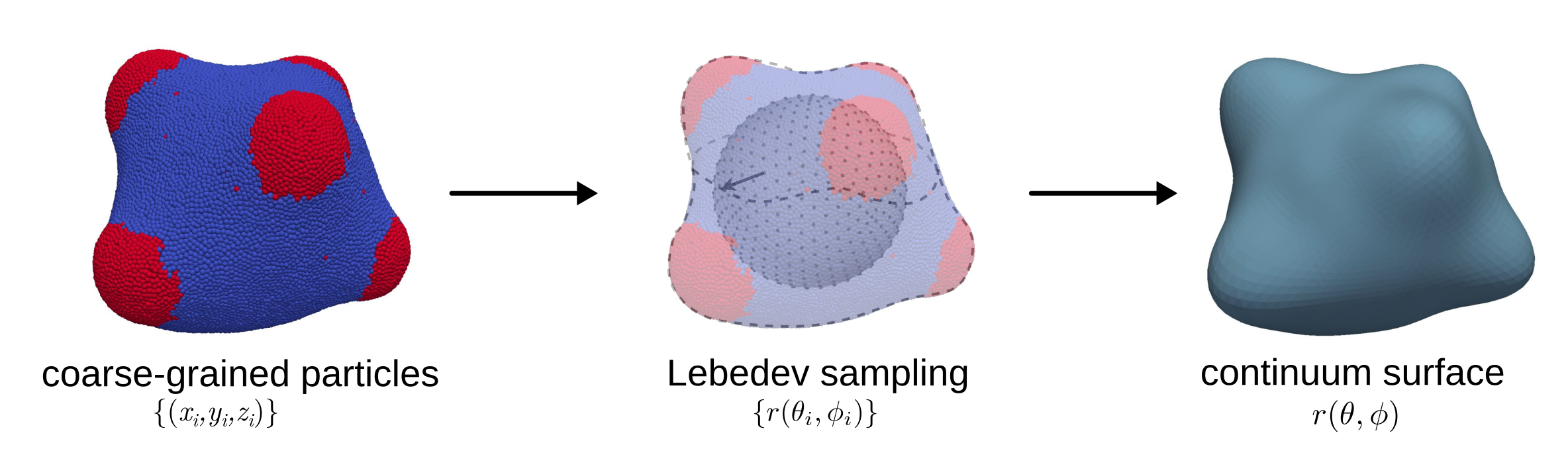
Figure 2: Mappings to the continuum representations. The collective configurations of the particles $\{(x_{i},y_{i},z_{i})\}$ are mapped to continuum representations using spherical harmonics expansions for the radial shape functions $r(\theta,\phi)$ in equation 11. Results are shown for $n=590$ Lebedev quadrature points for harmonics with degree $\ell\leq 21$.

4.1 Continuum Surface Representations: Spherical Harmonics Expansions

We represent the membrane surface in terms of the position function $\boldsymbol{r}(\theta,\phi)=r(\theta,\phi)\hat{\mathbf{e}}(\theta,\phi)\sigma$. The $\theta$ denotes the polar angle and $\phi$ the azimuthal angle for the spherical coordinate chart, $\hat{\mathbf{e}}(\theta,\phi)$ denotes the corresponding vector on the unit sphere, and $\sigma$ denotes our length-scale. The radial component $r$ of the function is expanded in spherical harmonics as

$$r(\theta,\phi;\boldsymbol{a})=\sum_{\ell,\hskip 2.84544pt|m|\leq\ell}a_{\ell m}Y_{\ell}^{m}(\theta,\phi),\;\;\;\;a_{\ell m}=\int_{\boldsymbol{r}}r(\theta,\phi)(Y_{\ell}^{m}(\theta,\phi))^{*}d\Omega.$$ (11)

The $Y_{\ell}^{m}$ denotes the spherical harmonic of degree $\ell$ and order $m$. The superscript $*$ denotes the complex conjugate. The $a_{\ell m}$ and expression in equation (11) gives the expansion coefficients for $r(\theta,\phi)$ in spherical harmonics. This can be viewed as the $L_{2}$-inner product $a_{\ell m}=\langle r(\theta,\phi),Y_{\ell}^{m}(\theta,\phi)\rangle_{L_{2}}$ over the sphere surface.

To approximate in practice the integration over the surface of the sphere and the inner-product, we use Lebedev quadratures [62, 61]. The Lebedev quadratures provide weights $w_{k}$ and nodal locations $\mathbf{x}_{k}$ to sample scalar functions $f$ on the spherical surface to approximate integrals as

$$\int f(\mathbf{x})d\Omega\sim\sum_{k=1}^{m}w_{k}f(\mathbf{x}_{k}).$$ (12)

The Lebedev quadratures have a number of desirable properties that include a high-order of accuracy and a more symmetric distribution of nodal samples than uniform latitude-longitude based methods [63, 60, 62].

We estimate the radial function $r(\theta_{k},\phi_{k})$ as $\tilde{r}_{k}$ using the coarse-grained beads comprising the membrane surface. This is computed using $\tilde{r}_{k}$ of a ray generated by the angles $(\theta_{k},\phi_{k})$. This is associated with the $k^{th}$ Lebedev quadrature node on the unit sphere. The coordinates of the closest bead to this ray is used on the surface. These calculations used $590$ Lebedev quadrature points to capture spherical harmonics of degree $\ell\leq 21$. The equation (11) is approximated by the discrete sum

$$\tilde{a}_{\ell m} =\sum_{k}w_{k}\tilde{r}_{k}.$$ (13)

The $w_{k}$ denotes the Lebedev quadrature weight associated with the $k^{th}$ node [62]. Equation 13 provides through the spherical harmonics expansion a continuum representation of the membrane surface geometry.

Our particle-to-continuum mapping is demonstrated in Figure 2. Here, the configuration is sampled from a two-phase membrane and the shape is reconstructed using the continuum representation based on spherical harmonics. Our approaches also can be used for the related problem of capturing the leading-order spherical harmonic modes representing other fields and hydrodynamic flows on surfaces of vesicles, see [63, 53, 54, 72, 60].

4.2 Bending Elasticity of Homogeneous Membranes

We consider the elasticity theory for homogeneous membranes introduced by Helfrich [73] and Canham [74] based on local mean and spontaneous curvatures. The free energy $E$ associated with membrane shape is

$$E[\boldsymbol{r}] =\int_{\boldsymbol{r}}\frac{k_{c}}{2}[2H(\theta,\phi;\boldsymbol{a})+c_{0}]^{2}dA+\lambda\int_{\boldsymbol{r}}dA.$$ (14)

The $k_{c}$ denotes the bending rigidity, $H$ the mean curvature, $c_{0}$ the spontaneous curvature, $dA$ the infinitesimal vesicle surface area, and $\lambda$ the tensile stress, serving as a Lagrange multiplier to maintain constant area.

We linearize the free energy in equation (14) in the case of vanishing spontaneous curvature $c_{0}=0$ around the reference configuration of a sphere and expand in spherical harmonics. In this case, the tensile stress term does not play a role in the second variation [75]. The free energy can be expressed in terms of spherical harmonics as

$$\tilde{E}[\mathbf{r}]=\tilde{E}[\{a_{\ell m}\}]=\frac{k_{c}}{2r_{0}^{2}}\sum_{\ell,m}|a_{\ell m}|^{2}\left[\ell(\ell+2)(\ell^{2}-1)\right].$$ (15)

The $a_{\ell m}$ denote the spherical harmonic expansion coefficients of the shape discussed in Section 4.1.

For physical vesicles comprised of molecular or particle constituents, the thermal undulations are modeled in equation (15) and [76] only up to the leading spherical harmonic modes above the molecular length-scales. Since the material is not a pure continuum, this results in aliasing artifacts in the harmonics description and for sufficiently small vesicles can result in what manifests as effective enhancement of the amplitudes of the fluctuations of harmonic modes.

Using the linearized theory of equation (15) to estimate a bending rigidity $k_{c}$ can then lead to an under-estimate of the mechanical rigidity. Helfrich derived correction terms to account for higher-order contributions in [76] giving the size-dependent effective bending rigidity

$$k_{c}^{\prime}=k_{c}-\frac{k_{B}T}{8\pi}\log{M}.$$ (16)

For spherical geometries, the $M$ represents half the number of amphilic molecules of a lipid bilayer membrane or more generally the number $N$ of particles comprising a leaflet of the membrane surface. The term involving $M$ can be viewed as an entropic contribution capturing neglected degrees of freedom of the system in the linearized elasticity theory such as higher-order contributions in the free energy [76]. The molecular parameter $M=N\approx\kappa 4\pi r_{0}^{2}$ is proportional to the area of the membrane surface. The equation (16) can be expressed as

$$\beta k_{c}^{\prime} =K-C\log{r_{0}},$$ (17)

where $\beta^{-1}=k_{B}T$. Within Helfrich’s theory for the area corrections of the linearized elasticity when treating vesicles as quasi-spherical [76], the coefficients would be $K=\beta k_{c}-\frac{1}{8\pi}\log{(\kappa 4\pi)}$ and $C={1}/{4\pi}$.

We expect more generally for other entropic effects to contribute to the elastic bending modulus with a similar scaling as equation (17). This would correspond to other values of $K$ and $C$. We show in Section 5.2 that such a scaling theory can be used with fit values of $K$ and $C$ to characterize how the estimated bending rigidity varies with the size of our coarse-grained vesicles.

4.2.1 Spherical Harmonics Conventions and Scale Separation

In practice, we have found it convenient to perform analysis using a real-valued spherical harmonics basis $X_{\ell}^{m}$, $Z_{\ell}^{m}$ expressed as $Y_{\ell}^{m}=X_{\ell}^{m}+iZ_{\ell}^{m}$ with $a_{\ell m}=\frac{1}{2}(x_{\ell m}-iz_{\ell m})$ for $m>0$ and $x_{\ell m},z_{\ell m}\in\mathbb{R}$. Since the membrane surface function is always real-valued, we have in the spherical harmonics representation that $a_{\ell m}=a_{\ell m}^{*}$, which requires that $x_{\ell m}=x_{l-m}$ and $z_{\ell m}=-z_{\ell-m}$. This allows us to express the radial function as

$$r(\theta,\phi) =\sum_{\ell=0}^{\infty}\sum_{m:-\ell\leq m\leq\ell}a_{\ell m}Y_{\ell}^{m}=\sum_{\ell=0}^{\infty}\big{[}a_{\ell,0}Y_{\ell}^{0}+\mkern-15.0mu\sum_{m:1\leq m\leq\ell}x_{\ell m}X_{\ell}^{m}+z_{\ell m}Z_{\ell}^{m}\big{]}.$$ (18)

This yields a real-valued basis comprised of $Y_{\ell}^{m}$ for $m=0$ and $X_{\ell}^{m}$, $Z_{\ell}^{m}$ for $\ell>0$, $m>0$. This has corresponding expansion coefficients $a_{\ell,0}$, $x_{\ell m}$ and $z_{\ell m}$ similar to [60, 72]. This can be related to our spherical harmonics expansion coefficients $a_{\ell m}$ by

$$a_{\ell m}=\begin{dcases}\frac{1}{2}(x_{\ell m}-iz_{\ell m}),&m>0\\ a_{\ell,0},&m=0\\ \frac{1}{2}(x_{\ell,|m|}-iz_{\ell,|m|}),&m<0.\end{dcases}$$ (19)

When considering the continuum mechanics which arises from the collective mechanics associated with the molecular interactions, it is important to consider the length-scales associated with the observed responses. This is especially important when length-scales approach molecular scales reaching the limits of a purely continuum interpretation. In the spectral analysis this corresponds to considering the length-scales associated with the different modal responses. To help with such interpretations, we develop relations between the key parameters to characterize spherical harmonics expansions and related spectral analysis.

Consider the characteristic length-scale of the particle/molecular interactions, which we denote by $d$. For our coarse-grained vesicle models, this is taken to be the bead size $d=\sigma$. For spherical harmonics expansions, this gives the critical wave-length associated with continuum responses of the system. One can think of the length $d$ as that of a small arc that is drawn along the equator of a sphere of radius $r_{0}$. For a quasi-spherical vesicle, the spherical harmonics expansion of equation (11) can be used to estimate the radius as $r_{0}={a_{00}}/{\sqrt{4\pi}}$. The $a_{00}$ is the coefficient of the constant mode. In spherical coordinates, the azimuthal angle is given by $\phi=d/r_{0}$. The spherical harmonic $Y_{\ell}^{m}$ has azimuthal angle dependence through the term $e^{im\phi}$. This has the largest spatial frequency when $m=\pm\ell$, giving the smallest wave-length resolved as $\lambda_{\ell}\sim r_{0}/m\sim r_{0}/\ell$.

In practice, for correspondence with continuum mechanics we should consider modes $\ell$ with $\lambda_{\ell}\gtrsim d$. When $d=\sigma$ is the bead size, we see this scaling analysis indicates that the local molecular or particle-level contributions start to dominate the spherical harmonics expansion when the harmonic degree $\ell$ is on the scale $\ell\sim r_{0}/d\sim r_{0}/\sigma$. This suggests the modes with $\ell\lesssim r_{0}/\sigma$ capture most significantly the responses of the system at the level of continuum mechanics. For larger degrees $\ell\gtrsim r_{0}/\sigma$, the modal responses depend more directly on signatures of the local molecular level interactions and noise. To relate the exhibited behaviors of our vesicles to continuum mechanics we shall focus on modal responses with $\ell\lesssim r_{0}/\sigma$.

4.2.2 Spectral Analysis of Passive Shape Fluctuations and Bending Elasticity

We use the passive thermal fluctuations of the vesicle shape to obtain information about the elastic bending modulus. From equilibrium statistical mechanics, the shape fluctuations are governed by the Gibbs-Boltzmann distribution

$$\rho[\{a_{\ell m}\}]=\frac{1}{Z}\exp\left(-E[\{a_{\ell m}\}]/k_{B}{T}\right),$$ (20)

where $Z$ represents the canonical partition function. Using the free energy of equation (15), the shape modes of $\rho[\{a_{\ell m}\}]$ have a Gaussian distribution with mean zero and variance

$$\mbox{Var}[a_{\ell m}]=\langle a_{\ell m}^{2}\rangle=\frac{r_{0}^{2}}{\beta k_{c}}\left[\ell(\ell+2)(\ell^{2}-1)\right]^{-1}.$$ (21)

The covariance between different modes is zero with $\mbox{Cov}[a_{\ell m},a_{\ell^{\prime}m^{\prime}}]=\langle a_{\ell m}a_{\ell^{\prime}m^{\prime}}\rangle=0$, where $\ell\neq\ell^{\prime}$, $m\neq m^{\prime}$. As $\ell$ becomes large, the variance scales as $\mbox{Var}[a_{\ell m}]\sim\ell^{-4}$. The equation (21) can be used to estimate the bending rigidity $k_{c}$ from the passive fluctuations of the vesicle.

In practice, we use the real-valued basis expansion of equation (18). We track $\text{Var}[a_{\ell,0}]$, $\text{Var}[x_{\ell m}]$ and $\text{Var}[z_{\ell m}]$ with $\ell>0$, $m>0$. When $\text{Cov}[x_{\ell m},z_{\ell m}]=0$, the variance can be expressed as

$$\text{Var}[a_{\ell m}]=\begin{dcases}\text{Var}[a_{\ell,0}],&m=0\\ \frac{1}{4}(\text{Var}[x_{\ell,|m|}]+\text{Var}[z_{\ell,|m|}]),&m\neq 0.\end{dcases}$$ (22)

When the variances are uncoupled for the different harmonic orders $m$, as in the elasticity theory of Section 4.2, averaging can be used to obtain

$$\langle a_{\ell}^{2}\rangle:=\frac{1}{2\ell+1}\sum_{|m|\leq\ell}\langle a_{\ell m}^{2}\rangle.$$ (23)

For spherical geometries in the basis expansion of Section 4.1, the mean is zero $\langle a_{\ell m}\rangle=0$ for $\ell\neq 0$. The bending rigidity $k_{c}$ is estimated by using a linear regression in $\log$-space with the estimator

$$\log{\langle a_{\ell}^{2}\rangle}=b-m\log{\left[\ell(\ell+2)(\ell^{2}-1)\right]}.$$ (24)

The $b=\log{(2r_{0}^{2}/\beta k_{c})}$ and $m=1$. In practice, the effective bending rigidity $k_{c}^{\prime}$ is estimated from equation (17). In Section 5.2, we showed that the empirical data exhibits the expected logarithmic scaling for the parameter values of $K$ and $C$ obtained from fitting simulations varying the vesicle size $r_{0}$.

5 Results

5.1 Phase Separation in Heterogeneous Vesicles

The heterogeneity of biological membranes and synthetic soft materials can play a significant role in shaping the geometry and in mechanical responses [15, 77, 2, 27, 25]. For both homogeneous and heterogeneous vesicles, we study how the mechanics depends on the concentration ratio and preferred curvatures of the phases. A few behaviors exhibited in our simulations are shown in Figure 3.

In our models the phase separation is driven primarily by the different species affinities, even when the preferred curvatures are the same. As the preferred curvature of the second phase is increased, it is found that the coarsening dynamics can stall given competition with curvature effects. The vesicles appear to exhibit meta-stable domains related to the elastic energy associated with the formation of bulged phase-separated domains. This results in a bending elasticity for the vesicle which presents a sufficiently large energy barrier inhibiting domains from further growth and merging during fluctuations. As the preferred curvature increases further, the coarsening dynamics were found to proceeds until a critical size, after which daughter vesicles bud from the vesicle. A few instances of these behaviors seen in our simulations are shown in Figure 3.

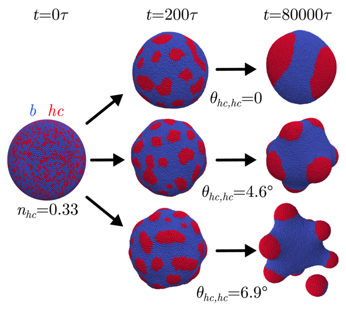
Figure 3: The preferred curvatures and phase separation are shown for a few cases. The phase preferred curvatures can impact coarsening and the vesicle shape. The top has matched curvatures between phases with $\theta_{hc,hc}\sim 0$ and the middle has intermediate differences. The bottom shows large differences where domains can form buds and daughter vesicles. The simulations consisted of $8000$ beads with $n_{hc}=0.33$, $k_{b}T=0.20\epsilon$, $\mu_{b,b}=3.0$, and $\mu_{b,hc}=6.0$.

In the case of a significant line tension, as opposed to a preferred curvature contrast, there can still be formation of buds or highly curved sub-domains. The parametrizations are considered where the line tensions are not sufficiently large to overcome the local bending energy. While the particle interactions are related in the coarse-grained potential, it is the local preferred curvature terms in the energy that drive the resulting geometry of our vesicles. For spherical topologies, the phase-separation will tend to proceed with the formation of two meta-stable domains at polar regions with the base phase in-between. This results in a large energy barrier inhibiting further merging into a single domain. In the intermediate regime with $\theta_{hc,hc}\sim 4.6$, the preferred curvature difference stalls the coarsening to yield many distinct sub-domains. We investigate both the passive shape fluctuations and mechanical responses to active deformations in Section 5.2– 5.5.

5.2 Homogeneous Vesicles and Size-Dependence of the Bending Elasticity

As a baseline for our studies, we first consider for homogeneous vesicles how their passive shape fluctuations and mechanical responses depend on the vesicle size.

In Helfrich [76], theory was developed for small vesicles predicting that the effective bending elasticity observed from shape fluctuations can depend significantly on the vesicle size. The coarse-grained models are used to further investigate the role of the vesicle size. We investigate the bending elasticity of homogeneous vesicles based on passive shape fluctuations using the methods developed in Section 4.2.2. The mechanical responses are considered over the range of sizes from $1255$ beads with $r_{0}\sim 9\sigma$ to $20088$ beads with $r_{0}\sim 36\sigma$. The surface area fluctuations are found to be less than $0.05\%$ for all sizes. For our coarse-grained vesicles, we show the scaling of the variances of the spherical harmonic modal responses $a_{\ell m}$ with degree $\ell$ in Figure 4.

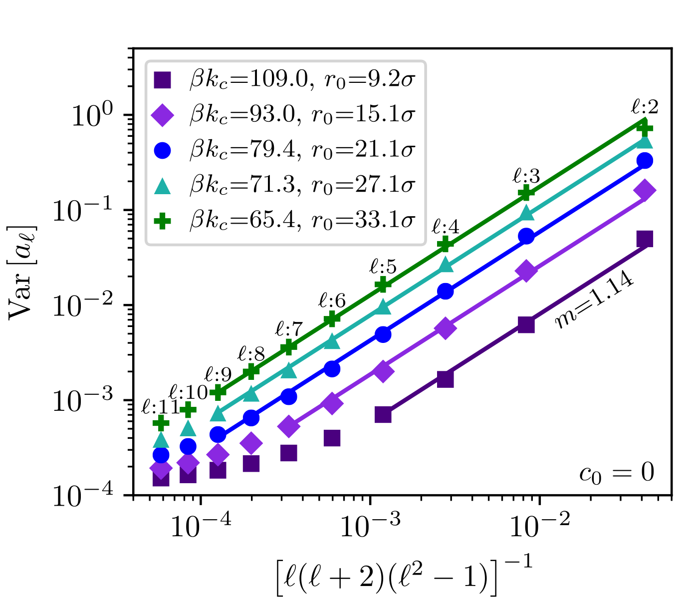
Figure 4: The fluctuation spectrum of vesicles of different sizes. For passive shape fluctuations mapped to harmonic modes of degree $\ell$, the variances are in good agreement with the continuum elasticity theory in equations(16), 23, and predictions by Helfrich [75]. Results are for $1000$ time-samples averaged over $5$ runs for each vesicle size.

The modes are averages over order $m$ as presented in equation (23). The linearized continuum elasticity theory predicts a scaling of $\mbox{Var}[a_{\ell m}]\sim\left[\ell(\ell+2)(\ell^{2}-1)\right]^{-1}$. While holding the particle interaction parameters fixed for the coarse-grained model, we find the estimated elastic bending modulus decreases as the size of the vesicle increases, see Figure 4.

For the linearized elasticity theory, entropy correction terms were derived for estimating the bending rigidity when varying the vesicle size [76]. The correction terms account for entropic contributions neglected in linear expansions. Our results show a similar trend with our coarse-grained vesicles having mechanical responses that exhibit a scaling similar to equation (17). The estimated bending modulus is shown in log-space as the vesicle size is varied, see Figure 5. We find a good fit is obtained for the scaling theory with the regression parameters $K=186.08$ and $C=34.70$ in equation (17).

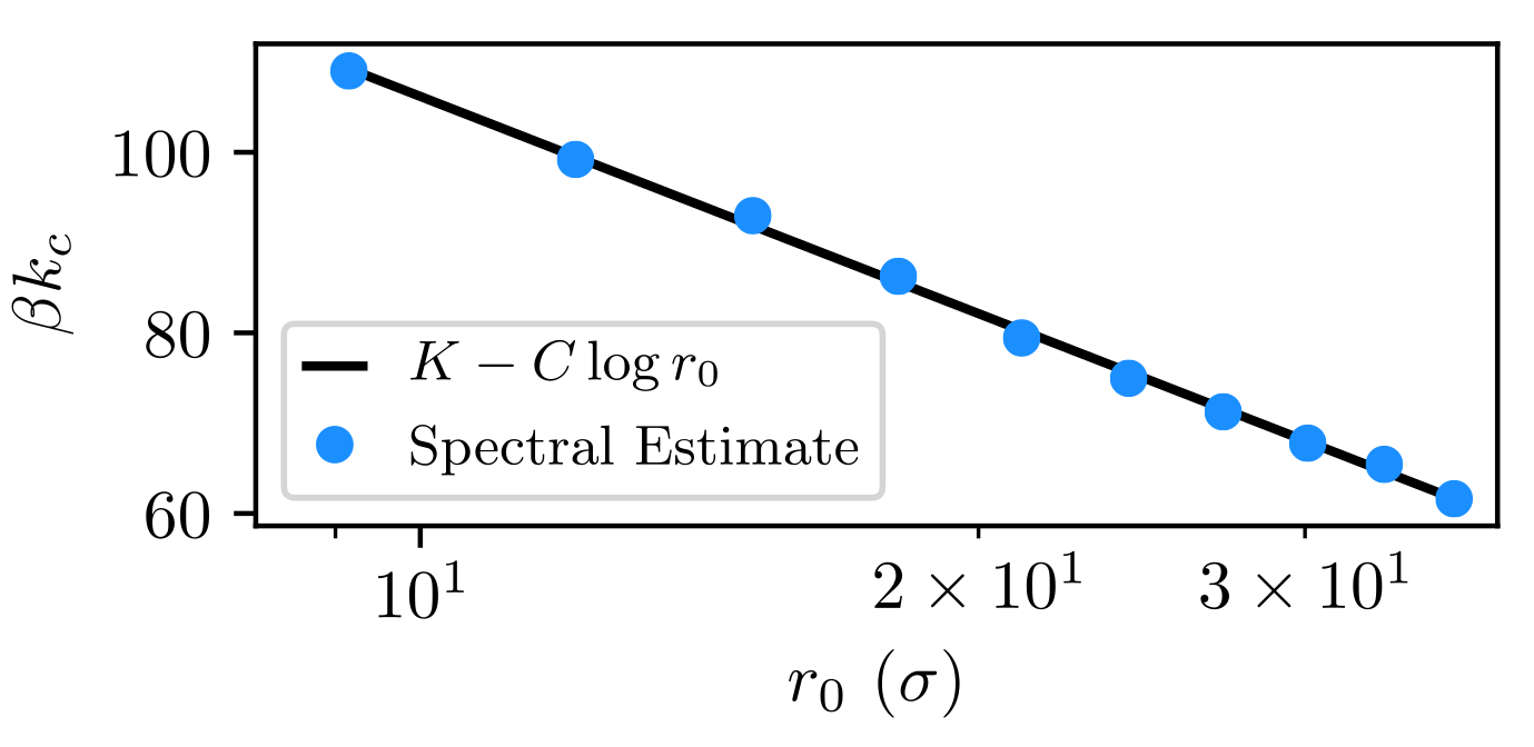
Figure 5: The bending elasticity for vesicles of different sizes. Shown is the elastic bending modulus exhibiting logarithmic scaling similar to the correction terms derived in Helfrich [75] and equation 16. The fitting parameters are $K=186.08$ and $C=34.70$.

5.3 Shape Fluctuations of Heterogeneous Vesicles

Heterogeneous vesicles are found to exhibit interesting spatial-correlations associated with sub-domain mechanics. This couples modes and makes traditional spectral analysis challenging. As an alternative we make comparisons using real-space two-point correlation functions of the undulations of the membrane surface for heterogeneous and homogeneous vesicles. The case is considered where heterogeneity occurs at scales comparable to the vesicle size. The shape fluctuations are characterized by the two-point correlations $\psi$ associated with the radial shape function $r(\theta,\phi)$.

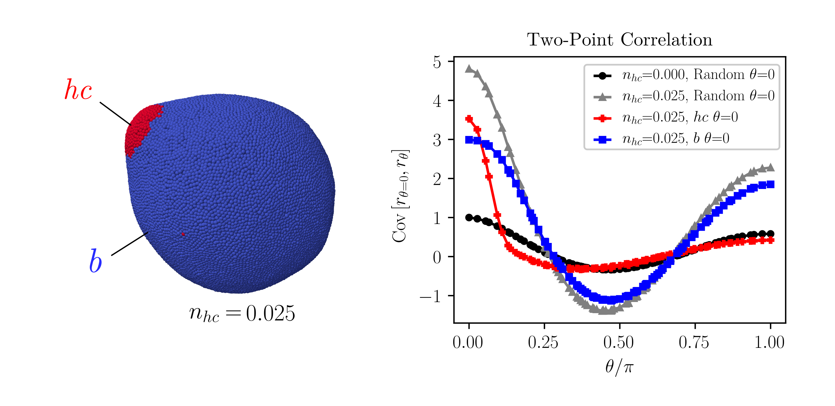
Figure 6: The surface two-point correlations are shown for the radial shape function $r(\theta,\phi)$ for homogeneous $n_{hc}=0$ and heterogeneous vesicles $n_{hc}>0$. The cases correspond to when the base-point is chosen (i) as any location at random on the surface, denoted “Random $\theta=0$”, (ii) to be within a high-curvature domain of phase $hc$, denoted “$hc\,\,\theta=0$”, and (iii) to be any point of the base phase $b$, denoted by “$b\,\,\theta=0$”. The base-point is taken to have coordinate $\theta=0$. Sampling was performed for $5$ random base-beads for 100 time-samples averaged over $5$ simulations runs. Results are normalized in scale by the variance at $\theta=0$ of the homogeneous vesicle.

The correlations are computed by choosing a base point for which the radial component is correlated with other points on the vesicle surface. There are three cases for choosing base-points, (i) as any location at random on the surface, denoted “Random $\theta=0$”, (ii) to be within a high-curvature domain of phase $hc$, denoted “$hc\,\,\theta=0$”, and (iii) to be any point of the base phase $b$, denoted by “$b\,\,\theta=0$”. The base-point is taken to have coordinate $\theta=0$. The case (i) is used primarily for homogeneous vesicles. The cases (i) and (ii) is used for the heterogeneous vesicles. The main difference is in case (ii) the base point is chosen within one of the phase-separated domains. This captures fluctuations within and in the vicinity of the domains of the vesicle. The results are normalized in scale by the variance at $\theta=0$ of the homogeneous vesicle.

In more detail, to obtain $\psi$ the chosen base-point can be thought of as being at the north pole of the vesicle with angles $(\theta_{0},\phi_{0})=(0,0)$. In practice, this is achieved by applying a rotation to the vesicle to transform it into this standard orientation. The base-point radial coordinate is then correlated with the other points of the vesicle at the polar angles $\theta$ by averaging the results over the azimuthal angle $\phi$. For the given case (i)–(iii) of base-point, this gives the two-point correlation function $\psi=\mbox{Cov}[r_{\theta=0}r_{\theta}]$. In practice, we approximate this by the estimator $\tilde{\psi}=1/N\sum_{i=1}^{N}r_{\theta=0}^{[i]}r_{\theta}^{[i]}-\bar{r}_{\theta=0}\bar{r}_{\theta}$. The $r_{\theta=0}^{[i]}$ is the $i^{th}$ sample of the base-point. The $r_{\theta}^{[i]}$ is the $i^{th}$ sample of the radius for any point with polar angle $\theta$. This is averaged over a sampling of base points consistent with one of the cases (i)–(iii). The $\bar{r}_{\theta}$ denotes the empirical mean of the radius of the points with polar angle $\theta$. Results for homogeneous vesicles with $n_{hc}=0.0$ and heterogeneous vesicles with $n_{hc}=0.025$ are shown in Figure 6.

It is found the two-point correlations for case (i) for both homogeneous and heterogeneous vesicles exhibit a strong negative correlation at around $\theta=\pi/2$. A strong positive correlation is also found at around $\theta=\pi$. These angles and correlations indicate significant ellipsoidal shape fluctuations in the overall geometry of the vesicles. This behavior also is seen to persist when also considering correlations at a base-point chosen in the base phase $b$, case (iii). When the base-points are chosen within the high-curvature domain of phase $hc$ (case (ii)), more complicated behaviors arise. The base-point plays an important role, since within the $hc$ regions it is sensitive to the local mechanics of the phase-separated domains. For the base-points in the $b$ regions characterizes locally the base-phase with more distant coupling to the phase domain mechanics. The correlations appear to be strongest within the high-curvature domain with relatively weak correlations with the regions of the base phase $b$, see Figure 6. The correlation functions are normalized by the $n_{hc}=0.0$ surface variance at $\theta=0$, $\mbox{Var}[r_{\theta=0}]=0.38$.

Our results for two-point correlations show some of the challenges inherent in developing estimators for the bending elasticity from a spectral analysis of shape fluctuations of heterogeneous vesicles. The heterogeneity breaks spatial symmetries resulting in coupling between spectral modes posing challenges for theory and analysis. Also, the phase domains can be of a comparable scale to the vesicle posing further issues. The phase domains have different local mechanical properties and can diffuse during fluctuations, undergo rearrangements, or merge. As an alterative for heterogeneous vesicles, we perform further simulations to actively drive deformations of the vesicles to better understand their mechanics and the roles of the phase domains.

5.4 Compression of Heterogeneous Vesicles: Mechanical Responses

In the molecular biology of cells, a central challenge is to understand the mechanisms by which cells sense and transduce mechanical stimuli into biochemical signals [78, 79, 3]. This includes both passive and active mechanical responses of cellular and sub-cellular structures [80, 81, 82, 13]. The coupling of chemical kinetics and mechanics is also important in the self-assembly and mechanical responses of synthetic soft materials [83, 84, 82, 25]. With the aim of understanding general principles, laboratory experiments and simulations have been performed with model physical systems. In [85], giant liposomes have been compressed between parallel plates to investigate force compression curves of the lipid membrane and in the presence or absence of an actin cortex. In [86], coarse-grained studies were performed for the relaxation times of homogeneous vesicles compressed by Atomic Force Microscopic (AFM) to obtain dependence on the applied force of the time-scale for stress relaxation.

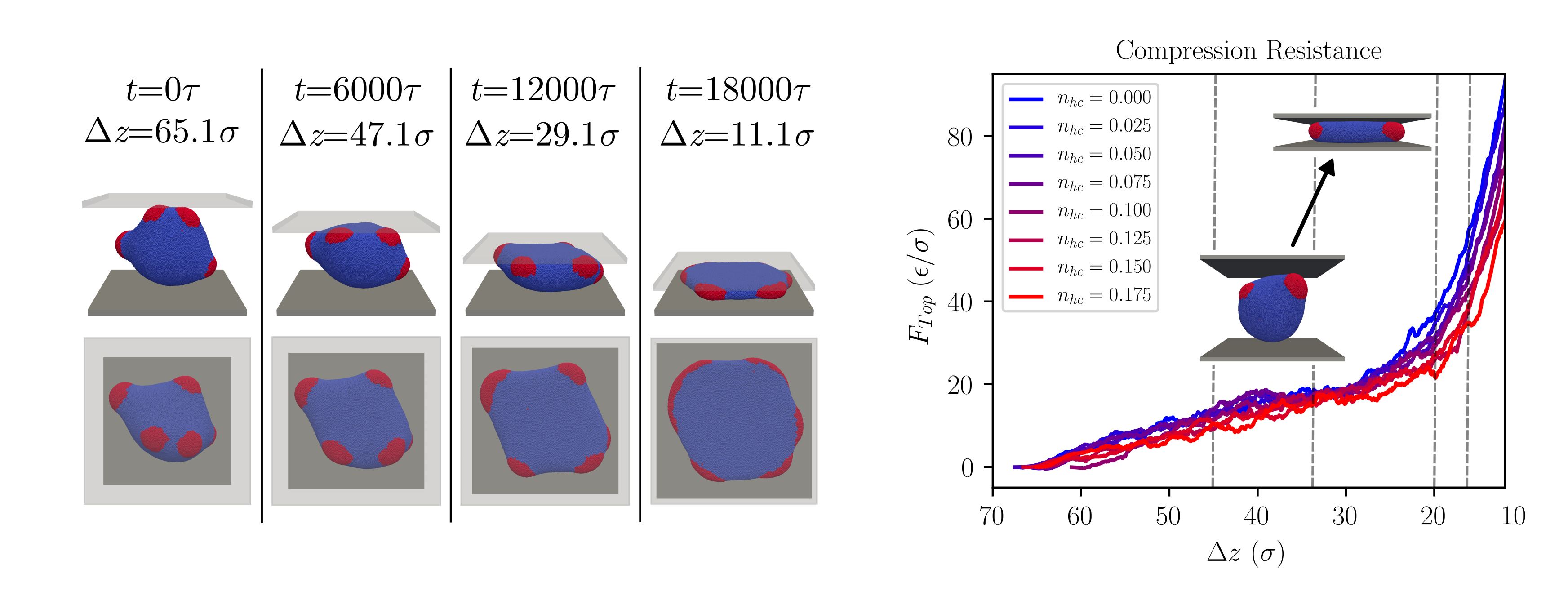
Figure 7: The compression forces of the deforming heterogeneous vesicles. A sample multi-phase vesicle is shown during different stages of compression when $n_{hc}=0.175$ (left). For vesicles with different phase mixtures $n_{hc}$, the resisting forces are shown (right). For the dashed lines at compressions $\Delta{z}=45\sigma,\Delta{z}=33\sigma$, $\Delta{z}=20\sigma$, and $\Delta{z}=16\sigma$, the force is compared for the different phase concentrations in Figure 9.

We perform studies to probe the mechanics of heterogeneous vesicles by compressing them between flat plates. A collection of representative meta-stable coarse-grained vesicles are used having varying levels of concentration for a high-curvature species. Vesicles of the type discussed in Section 5.1 are used with $\theta_{hc,hc}=5.73^{\circ}$. The specific concentrations considered are $n_{hc}=0.025k$, where $k=0,1,2,...,7$. The $n_{hc}$ gives the percentage of high-curvature species in the membrane. Our equilibrated non-spherical vesicles have a size characterized by the expansion coefficient $a_{00}$ for the harmonic mode $Y_{0}^{0}$ as in Section 4.2.1. Our vesicles have similar characteristic radius $r_{0}$ ranging from $r_{0}\sim 30.1\sigma$ for $n_{hc}=0.0$ to $r_{0}\sim 28.9\sigma$ for $n_{hc}=0.175$. Vesicles are compressed by moving a top wall downward toward a stationary wall below. The top wall is moved at a constant speed of $v=0.003\sigma/\tau$. The steric particle-wall interactions are modeled by a 9-3 LJ-potential with depth $\epsilon_{\text{wall}}=0.01\epsilon$ with length-scale $\sigma_{\text{wall}}=\sigma$. The particle-wall force is computed using the approach in Appendix B.

During compression, the high-curvature phase domains rearrange to be parallel to the walls around the free perimeter of the flattening vesicle, see Figure 7. For heterogeneous structures arising in cell biology, the rearrangement of such protruding domains could provide potential mechanisms for mechanosensing large compressive deformations. During most of the compression, the homogeneous and heterogeneous vesicles take on overall ellipsoidal-like shape with similar $Y$ modes. However, the shape mode $x_{22}$ differs significantly for the heterogeneous case given the role of the phase domains, see Figure 8. While the overall shapes following similar trends, the heterogeneous vesicles can accommodate better the stresses associated with the large deformations by rearrangement of the high-curvature preferring domains towards the areas of larger curvature. This results in a lower energetic cost for the deformation and smaller resistance forces since the high-curvature domains rearrange to occupy bending regions at their preferred curvatures, see Figure 9 and Figure 7.

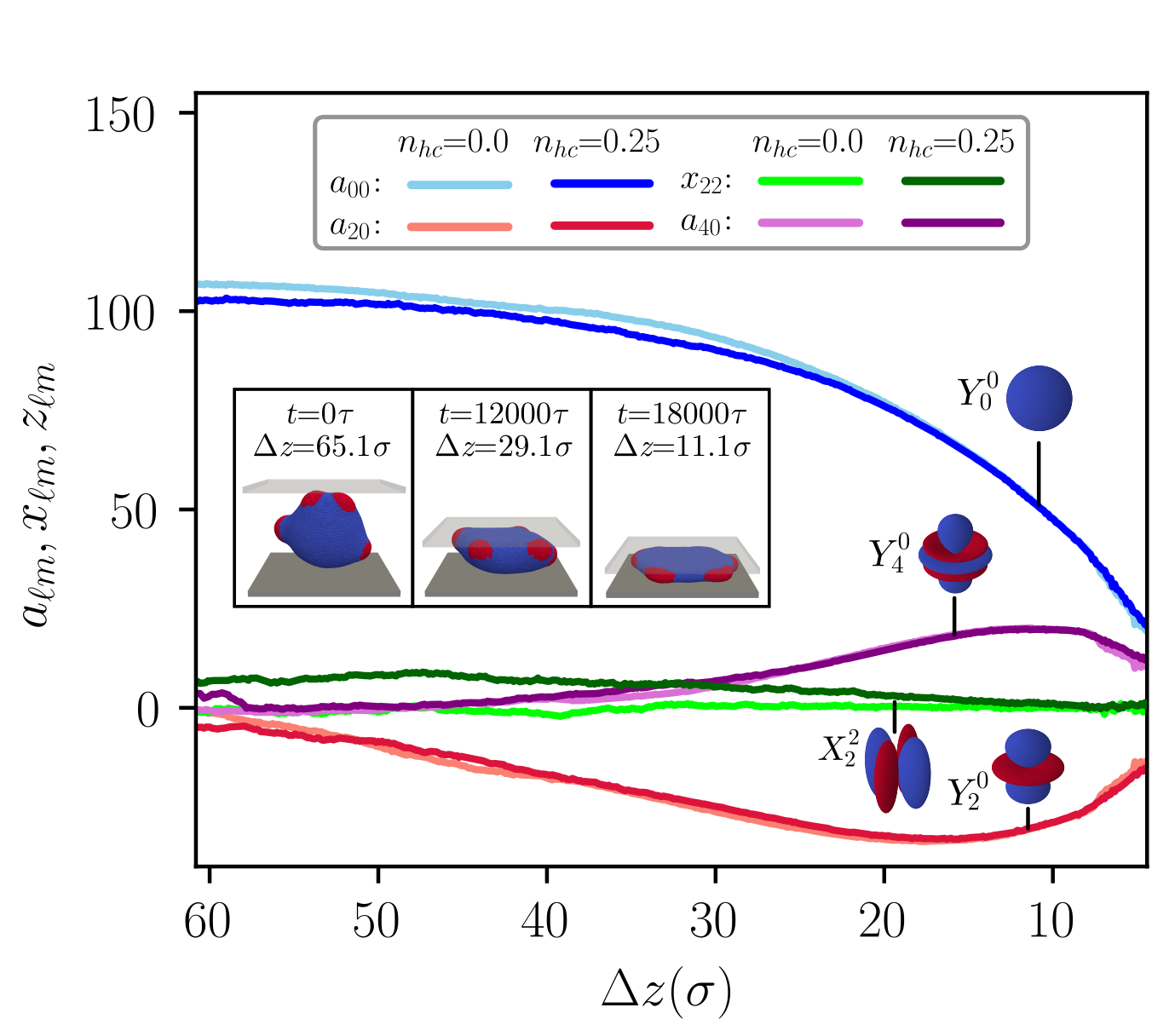
Figure 8: The shape changes and domain rearrangements during compression. For vesicles with $n_{hc}=0$ and $n_{hc}=0.175$, the shape changes are characterized by select spherical harmonic modes with coefficients $a_{00}$, $a_{20}$, $x_{22}$, and $a_{40}$. These correspond to the real-valued harmonics shown as radial shapes with blue for positive and red for negative values for $Y_{0}^{0}$, $Y_{2}^{0}$, $X_{2}^{2}$, and $Y_{4}^{0}$.

We investigate the resisting forces the vesicles exert on the walls as the level of heterogeneity increases in Figure 9. It is found the resisting forces the vesicle exerts on the walls decreases as the level of heterogeneity increases. As the compression becomes larger, and the shape more pancake-like, both the high-curvature domains and base phase deform significantly. A significant decrease occurs in the resisting force for the heterogeneous vesicles as the concentration of the high-curvature species increases, see Figure 9. These results show some of the ways in which the phase-separated domains can contribute to mechanical responses of heterogeneous vesicles.

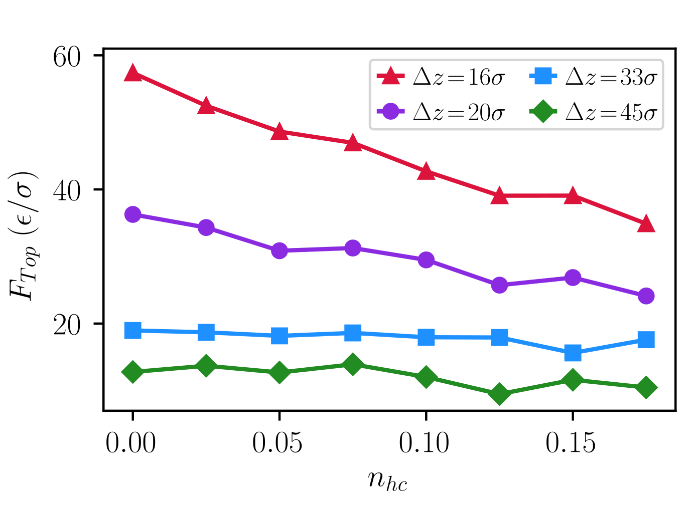
Figure 9: The compression forces of the deforming heterogeneous vesicles. Shown is the $z$-component of the resistance force when varying the concentration $n_{hc}$. The $\Delta{z}$ indicates the wall-separation distance.

5.5 Insertion and Transport of Heterogeneous Vesicles within Channels

The mechanics and kinetics of heterogeneous structures inserting into small capillaries, pores, or channels play an important in cellular processes and microfluidic devices [87, 88, 89]. Toward understanding general principles, model physical systems have been studied [90, 91]. In [90], a microfluidics model system was developed to investigate the role of elastic mechanics of red blood cells in traversing micro-capillaries when in healthy states and when in diseased states, such as malaria which has increased rigidity. In [91], the permeation of homogeneous vesicles through narrow pores was studied with an emphasis on the roles of surface adhesion, elasticity, and surface tension on the pressure differences required to drive transport through pores.

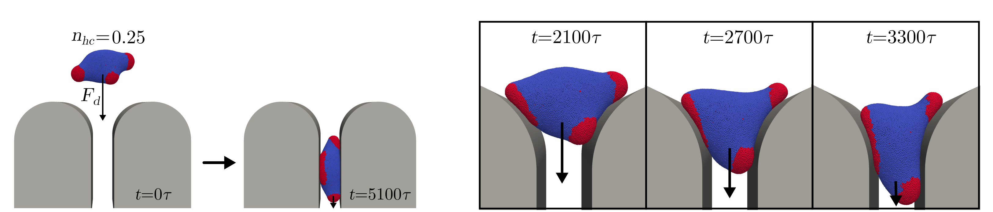
Figure 10: Heterogeneous vesicles inserting into channels. Vesicles experience a constant pressure load force $\boldsymbol{F}_{d}=-(0.015\epsilon/\sigma)\hat{\boldsymbol{z}}$ that drives insertion and transport within slit-like channels. The channels have wall-separation distance $30\sigma$ with an entrance smoothed by a cylinder having radius $50\sigma$ (left). The vesicle significantly deforms and rearranges phase domains during insertion into the channel opening (right). Results for vesicle transit times are shown in Figure 12.

We investigate the behaviors of heterogeneous vesicles when inserted and transported within slit-like channels. The vesicle kinetics of insertion and transport are studied when varying the concentration of the high-curvature phase. The hydrodynamics is treated as a simplified model with a constant drag and pressure force acting on all particles of the vesicle. This is motivated by the hypothesis that as opposed to flow the insertion process is driven primarily by surface pressures of the incompressible fluid transmitted over the membrane surface of the vesicles. Other approaches, such as fluctuating hydrodynamics methods incorporating more detailed fluid mechanics could also be used to extend our coarse-grained model as in [59]. The driving force is taken to be $\boldsymbol{F}_{d}=-(0.015\epsilon/\sigma)\hat{\boldsymbol{z}}$. The channel geometry consists of two plates with separation distance $30\sigma$. The channel entrance is smoothed by two cylinders, both of radius $50\sigma$. At the start, vesicles have effective radii ranging from $r_{0}\sim 30.1\sigma$ for $n_{hc}=0.0$ to $r_{0}\sim 26.0\sigma$ for $n_{hc}=0.3$, as determined from the $a_{00}$ basis-expansion coefficient corresponding to spherical harmonic mode $Y_{0}^{0}$. The channel and some typical configurations of the vesicles before, during, and after insertion are shown in Figure 10.

We compare for homogeneous and heterogeneous vesicles how the different concentrations of the high-curvature phase impact the distance $z(t)$ the vesicles are transported within the channel over time duration $t$. The distance of the homogeneous vesicle is denoted by $z_{0}(t)$. We report the lag-distance $\Delta{z}_{lag}=z(t;n_{hc})-z_{0}(t)$ between the position $z(t;n_{hc})$ of the heterogeneous vesicle and the homogeneous case. The trials are averaged over $10$ random initial orientations for each vesicle. We report our results in Figure 12.

It was found the heterogeneous vesicles had longer transport times and larger variances in the channel insertion studies. These vesicles enter the channel through a combination of rearrangement of the phase domains, further deformation-driven phase coarsening, and changes in the shape. Since the vesicles have non-spherical shapes, the initial orientations when encountering the channel entrance also can play a role, see Figure 10. From our discrete-to-continuum mappings these shape changes were quantified in terms of modes in Figure 11. Relative to the homogeneous case, we found there were significant differences seen in the shapes during the insertion phase. By the time $t=3900\tau$, all of the vesicles were fully inserted within the channel and took on similar overall ellipsoidal shapes. For heterogeneous vesicles, this combination of effects were found to lead to significant differences in transport times and insertion kinetics relative to the homogeneous case, see Figs. 10–12.

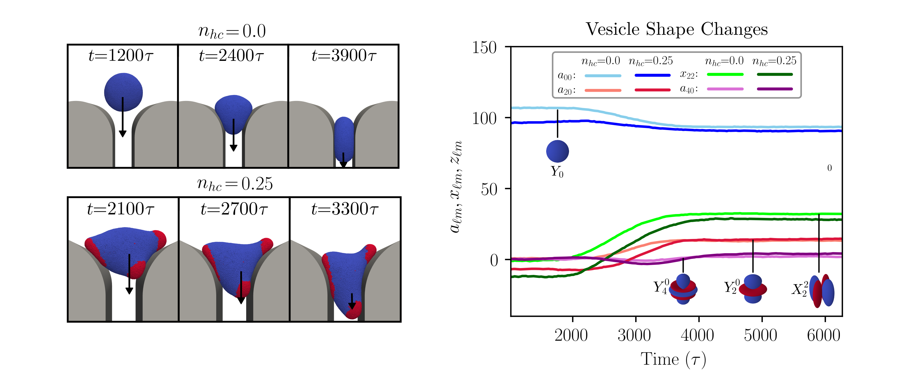
Figure 11: The vesicle shape changes during insertion into channels. The changes are compared for a heterogeneous vesicle relative to the homogeneous case (left). The changes in shape of vesicles is characterized using the spherical harmonics with coefficients $a_{00}$, $a_{20}$, $x_{22}$, and $a_{40}$. The harmonics are shown as radial functions with blue positive and red negative for the modes $Y_{0}^{0}$, $Y_{2}^{0}$, $X_{2}^{2}$, and $Y_{4}^{0}$ (right)

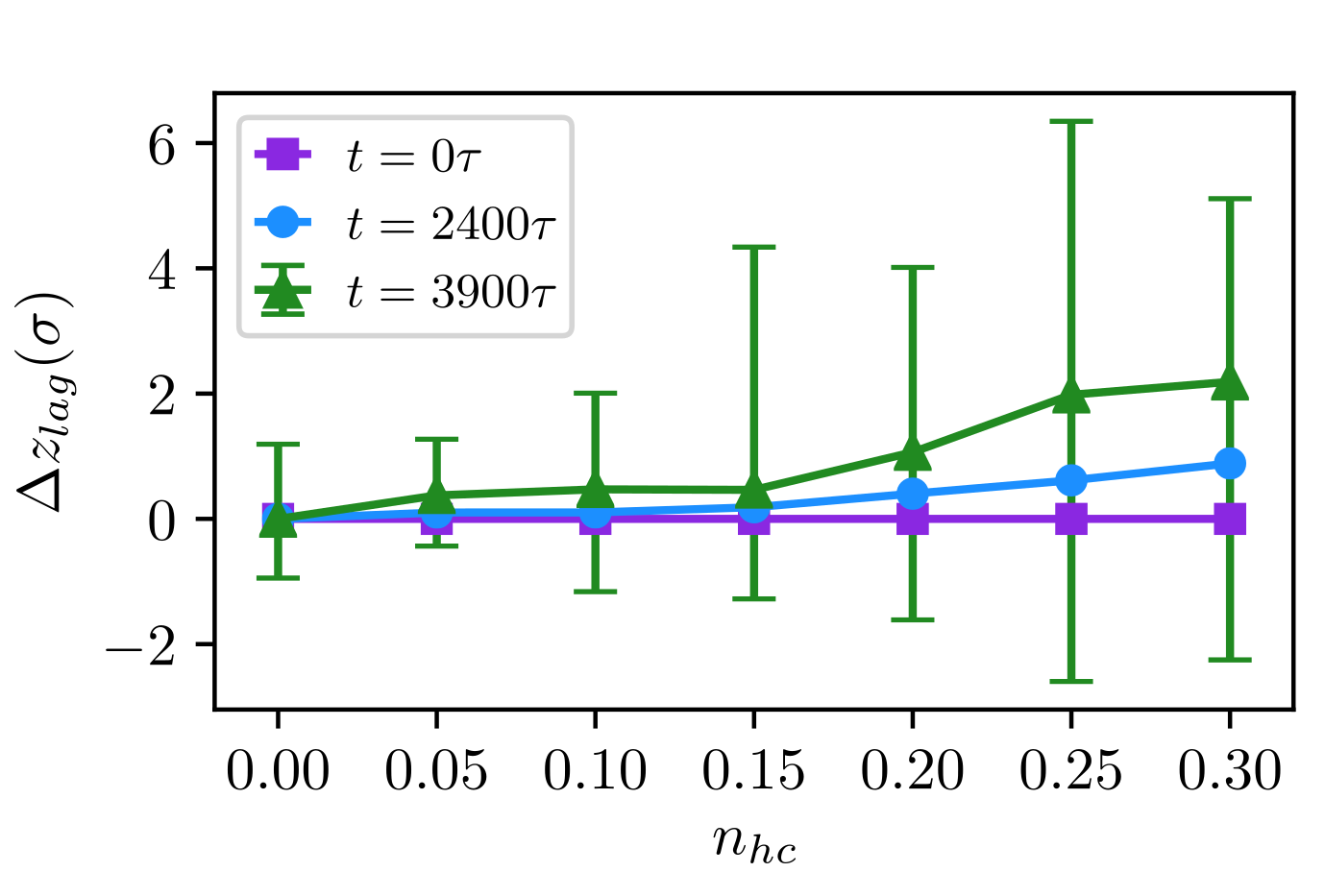
Figure 12: The vesicle shape changes during insertion into channels. For vesicles with different phase mixtures $n_{hc}$, the distance $z(t)$ is shown for how far a vesicle has traveled down the channel by time $t$. The lag-distance $\Delta{z}_{lag}=z(t;n_{hc})-z_{0}(t)$ is reported for the position $z(t;n_{hc})$ of the heterogeneous vesicle compared with the homogeneous case $z_{0}(t)$. Results are averaged over $10$ simulations for vesicles with random initial orientations. For the case $t=3900\tau$, when all vesicles were fully inserted into the channel, bars are shown indicating the range of the smallest and largest lags observed over the trials.

It was interesting that while the heterogeneous vesicles could better accommodate deformations during compression incurring a lower energetic cost, they still took more time on average to insert into channels. This appears to be a consequence of the sequential nature of the insertion process. During insertion only the leading part of the vesicle is initially subjected to deformation. Depending on the initial vesicle orientation and arrangement of the phase domains, this could delay insertion, given the need for phase domains to rearrange to accommodate the deformations required for full insertion into the channel. This is seen in the large variability of the insertion times, with the heterogeneous case sometimes occurring more rapidly or much more slowly than the homogeneous case, see Figure 12. The simulation results for the heterogeneous vesicles show how many of the behaviors differ significantly relative to their homogeneous counter-parts.

6 Conclusions

Heterogeneous vesicles with membranes having phase-separated domains can exhibit interesting mechanical responses and other behaviors differing significantly from homogeneous vesicles. Our coarse-grained simulation and analysis methods allow for better understanding the roles played by the phase-separated domains both in passive shape fluctuations and during active deformations. Our discrete-to-continuum mapping methods and spherical harmonics approaches allow for relating configurations in coarse-grained descriptions to corresponding continuum fields providing quantitative characterizations. For shape fluctuations when varying the vesicle sizes, we showed how this could be used to make comparisons with theory based on continuum mechanics. We further showed the phase-separated domains break rotational symmetries resulting in passive shape fluctuations and two-point correlations having enhanced amplitude and variability relative to the homogeneous case. We also showed how our approaches can be used to probe mechanical responses when subjected to more active deformations. When compressing vesicles between two plates, we found the high-curvature phases can rearrange to accommodate bending stresses by distributing near the most curved edges of the compressing vesicle. For studies of vesicle insertion into channels, we further found that the heterogeneity can have mixed results. When the orientation of the vesicle had the ellipsoidal major axis aligned with the channel, we found heterogeneous vesicles can insert rapidly. However, when the orientation is orthogonal, we found delays can arise from deformations and rearrangements of the phase-separated domains during vesicle insertion into the channel. This manifested as significant variability in transport times. These results suggest a few novel mechanisms by which membrane heterogeneity can augment membrane mechanics and kinetics. Our introduced methods provide ways to quantitatively characterize these differences. Our methods provide general approaches for further investigations of phenomena within heterogeneous membranes taking into account the roles played by phase separation, thermal fluctuations, geometry, and mechanics. Our results show that the presence of even a modest number of phase-separated domains in heterogeneous membranes can significantly augment their mechanical responses relative to the homogeneous case.

Appendix A Gradients of the Energy $U(\mathbf{r}_{ij},\mathbf{n}_{i},\mathbf{n}_{j})$

The detailed expressions are given for each of the gradients of the potential energy with respect to the translational $\mathbf{r}$ and rotational $\mathbf{n}_{i}$ degrees of freedom contributing in equation1. These gradients can be expressed as

$$\nabla_{\mathbf{r}_{i}}U = \begin{cases}\nabla_{\mathbf{r}_{i}}u_{R}(r)-\epsilon\mu\nabla_{\mathbf{r}_{i}}a&\quad r<r_{b}\\ \phi\nabla_{\mathbf{r}_{i}}u_{A}(r)+u_{A}(r)\mu\nabla_{\mathbf{r}_{i}}a&\quad r_{b}<r<r_{c}\end{cases}$$ (25)

$$\nabla_{\mathbf{n}_{i}}U = \begin{cases}-\epsilon\mu\nabla_{\mathbf{n}_{i}}a&\quad r<r_{b}\\ u_{A}(r)\mu\nabla_{\mathbf{n}_{i}}a&\quad r_{b}<r<r_{c}\end{cases}$$ (26)

$$\nabla_{\mathbf{r}_{i}}u_{R}(r) = -\frac{4\epsilon}{r_{b}}\bigg{[}\Big{(}\frac{r_{b}}{r}\Big{)}^{5}-\Big{(}\frac{r_{b}}{r}\Big{)}^{3}\bigg{]}\mathbf{\hat{r}}_{ij}$$ (27)

$$\nabla_{\mathbf{r}_{i}}u_{A}(r) = \frac{\epsilon\pi\zeta}{(r_{c}-r_{b})}\cos^{2\zeta-1}(\xi)\sin(\xi)\mathbf{\hat{r}}_{ij},\quad\xi=\frac{\pi}{2}\frac{(r-r_{b})}{(r_{c}-r_{b})}$$ (28)

$$\nabla_{\mathbf{r}_{i}}a = \frac{1}{r}\big{[}2(\mathbf{n}_{i}\cdot\mathbf{\hat{r}}_{ij})(\mathbf{n}_{j}\cdot\mathbf{\hat{r}}_{ij})\mathbf{\hat{r}}_{ij}-(\mathbf{n}_{i}\cdot\mathbf{\hat{r}}_{ij})\mathbf{n}_{j}-(\mathbf{n}_{j}\cdot\mathbf{\hat{r}}_{ij})\mathbf{n}_{i}$$

$$- \sin\theta_{0}\big{(}\mathbf{n}_{j}-\mathbf{n}_{i}-[(\mathbf{n}_{j}-\mathbf{n}_{i})\cdot\mathbf{\hat{r}}_{ij}]\mathbf{\hat{r}}_{ij}\big{)}\big{]}$$

$$\nabla_{\mathbf{n}_{i}}a = \mathbf{n}_{j}-(\mathbf{n}_{j}\cdot\mathbf{\hat{r}}_{ij}-\sin\theta_{0})\mathbf{\hat{r}}_{ij}.$$ (30)

Appendix B Computing the Wall-Force: Resistance of Vesicles to Compression

For compression of the vesicles between the two walls, we compute the effective wall-force, related to the pressure, exerted by the vesicle on the walls. Consider the geometry of a wall $w$ spanning the $xy$-plane at $z=z_{w}$. Let $z_{i}$ denote the $z$-position of the $i^{th}$ particle. Consider the free-energy of the particle-wall interaction $U_{w}(z_{i}-z_{w})$, which in our studies is a 9-3 LJ-potential. The force exerted by the $i^{th}$ particle on the wall is given by $\tilde{F}_{w,i}=-\nabla_{z_{w}}U_{w}(z_{i}-z_{w})$. For our studies of compression, we sum over all of the vesicle’s particles with $|z_{i}-z_{w}|<2.5\sigma$ to obtain the total particle-wall force

$$F_{w}=-\sum_{i}\nabla_{z_{w}}U_{w}(z_{i}-z_{w}).$$ (31)

In our studies, the bottom wall is stationary, so we use the wall separation $z=z_{Top}-z_{Bottom}$ to parameterize the force $F_{Top}(z)$. We use this approach to compute the reported resisting forces when compressing homogeneous and heterogeneous vesicles between the planar walls in Section 5.4.

References

- [1] S.. Singer and Garth L. Nicolson “The Fluid Mosaic Model of the Structure of Cell Membranes” In Science 175.4023, 1972, pp. 720–731 URL: http://www.sciencemag.org/content/175/4023/720.abstract
- [2] D. Lingwood and K. Simons “Lipid Rafts As a Membrane-Organizing Principle” In Science 327, 2010, pp. 46–50 DOI: 10.1126/science.1174621
- [3] B. Alberts et al. “Molecular Biology of the Cell” Garland Publishing, 2002
- [4] Florly S. Ariola et al. “Membrane Fluidity and Lipid Order in Ternary Giant Unilamellar Vesicles Using a New Bodipy-Cholesterol Derivative” In Biophysical Journal 96, 2009, pp. 2696–2708 DOI: 10.1016/j.bpj.2008.12.3922
- [5] Sarah L. Veatch and Sarah L. Keller “Separation of Liquid Phases in Giant Vesicles of Ternary Mixtures of Phospholipids and Cholesterol” In Biophysical Journal 85, 2003, pp. 3074–3083 DOI: 10.1016/s0006-3495(03)74726-2
- [6] Stefan Semrau, Timon Idema, Thomas Schmidt and Cornelis Storm “Membrane-mediated interactions measured using membrane domains” In Biophysical journal 96.19527649 The Biophysical Society, 2009, pp. 4906–4915 URL: https://www.ncbi.nlm.nih.gov/pmc/PMC2712058/
- [7] Yoshihisa Kaizuka and Jay T. Groves “Bending-mediated superstructural organizations in phase-separated lipid membranes” In New Journal of Physics 12.9, 2010, pp. 095001 URL: http://stacks.iop.org/1367-2630/12/i=9/a=095001
- [8] François Quemeneur et al. “Shape matters in protein mobility within membranes” In Proceedings of the National Academy of Sciences 111.14 National Acad Sciences, 2014, pp. 5083–5087
- [9] A.. Lee “Lipid–protein interactions in biological membranes: a structural perspective” In Biochimica et Biophysica Acta (BBA) - Biomembranes 1612.1, 2003, pp. 1–40 URL: http://www.sciencedirect.com/science/article/pii/S0005273603000567
- [10] Michael Edidin “The State of Lipid Rafts: From Model Membranes to Cells” In Annu. Rev. Biophys. Biomol. Struct. 32.1 Annual Reviews, 2003, pp. 257–283 DOI: 10.1146/annurev.biophys.32.110601.142439
- [11] A.. Lee “Annular events: lipid-protein interactions” In Trends in Biochemical Sciences 2.10, 1977, pp. 231–233 URL: http://www.sciencedirect.com/science/article/pii/0968000477901177
- [12] Gary J. Doherty and Harvey T. McMahon “Mediation, Modulation, and Consequences of Membrane-Cytoskeleton Interactions” In Annual Review of Biophysics 37.1 Annual Reviews, 2008, pp. 65–95 URL: http://dx.doi.org/10.1146/annurev.biophys.37.032807.125912
- [13] Tomas Kirchhausen “Clathrin” In Annual Review of Biochemistry 69.1 Annual Reviews, 2000, pp. 699–727 URL: http://dx.doi.org/10.1146/annurev.biochem.69.1.699
- [14] H.G. Döbereiner et al. “Budding and fission of vesicles” In Biophysical Journal 65.4, 1993, pp. 1396–1403 URL: http://www.sciencedirect.com/science/article/pii/S0006349593812037
- [15] Tobias Baumgart, Samuel T Hess and Watt W Webb “Imaging coexisting fluid domains in biomembrane models coupling curvature and line tension” PMID: 20636098 In Nature 425.6960, 2003, pp. 801–832 URL: https://www.nature.com/articles/nature02013
- [16] Harvey T. McMahon and Jennifer L. Gallop “Membrane curvature and mechanisms of dynamic cell membrane remodelling” In Nature 438 Nature Publishing Group, 2005, pp. 590 URL: https://doi.org/10.1038/nature04396
- [17] G. Oster, H. Moore and A. Goldbeter “The budding of membranes” In Cell to Cell Signalling Academic Press, 1989, pp. 171–187 URL: http://www.sciencedirect.com/science/article/pii/B9780122879609500204
- [18] Touko Apajalahti et al. “Concerted diffusion of lipids in raft-like membranes” In Faraday Discuss. 144 The Royal Society of Chemistry, 2010, pp. 411–430 URL: http://dx.doi.org/10.1039/B901487J
- [19] Jay T. Groves, Raghuveer Parthasarathy and Martin B. Forstner “Fluorescence Imaging of Membrane Dynamics” In Annu. Rev. Biomed. Eng. 10.1 Annual Reviews, 2018, pp. 311–338 DOI: 10.1146/annurev.bioeng.10.061807.160431
- [20] Jonas Korlach, Tobias Baumgart, Watt W. Webb and Gerald W. Feigenson “Detection of motional heterogeneities in lipid bilayer membranes by dual probe fluorescence correlation spectroscopy” In Biochimica et Biophysica Acta (BBA) - Biomembranes 1668.2, 2005, pp. 158–163 URL: http://www.sciencedirect.com/science/article/pii/S0005273604003116
- [21] Rebecca D. Usery et al. “Membrane Bending Moduli of Coexisting Liquid Phases Containing Transmembrane Peptide” In Biophysical Journal 114.9, 2018, pp. 2152–2164 URL: http://www.sciencedirect.com/science/article/pii/S0006349518303953
- [22] Edward Barry and Zvonimir Dogic “Entropy driven self-assembly of nonamphiphilic colloidal membranes” In Proceedings of the National Academy of Sciences 107.23 National Academy of Sciences, 2010, pp. 10348–10353 DOI: 10.1073/pnas.1000406107
- [23] A.. Dinsmore et al. “Colloidosomes: Selectively Permeable Capsules Composed of Colloidal Particles” In Science 298, 2002, pp. 1006–1009 DOI: 10.1126/science.1074868
- [24] Tobias Bollhorst, Kurosch Rezwan and Michael Maas “Colloidal capsules: nano- and microcapsules with colloidal particle shells” In Chem. Soc. Rev. 46, 2017, pp. 2091–2126 DOI: 10.1039/C6CS00632A
- [25] Prerna Sharma et al. “Hierarchical organization of chiral rafts in colloidal membranes” In Nature 513 Nature Publishing Group, a division of Macmillan Publishers Limited. All Rights Reserved., 2014, pp. 77 URL: https://doi.org/10.1038/nature13694
- [26] Sangwoo Kim and Sascha Hilgenfeldt “Heterogeneous vesicles: an analytical approach to equilibrium shapes” In Soft Matter 11.46, 2015, pp. 8920–8929
- [27] KyuHan Kim, Siyoung Q. Choi, Joseph A. Zasadzinski and Todd M. Squires “Interfacial microrheology of DPPC monolayers at the air-water interface” In Soft Matter 7, 2011, pp. 7782–7789 DOI: 10.1039/C1SM05383C
- [28] Reinhard Lipowsky and Rumiana Dimova “Domains in membranes and vesicles” In Journal of Physics: Condensed Matter 15.1, 2003, pp. S31 URL: http://stacks.iop.org/0953-8984/15/i=1/a=304
- [29] Frank Juilcher and Reinhard Lipowsky “Domain-induced budding of vesicles” In PRL 70.19 American Physical Society, 1993, pp. 2964–2967 URL: https://link.aps.org/doi/10.1103/PhysRevLett.70.2964
- [30] D Andelman, T Kawakatsu and K Kawasaki “Equilibrium Shape of Two-Component Unilamellar Membranes and Vesicles” In Europhysics Letters (EPL) 19.1 IOP Publishing, 1992, pp. 57–62 DOI: 10.1209/0295-5075/19/1/010
- [31] M Laradji, H Guo, M Grant and M J Zuckermann “Dynamics of phase separation in the presence of surfactants” In Journal of Physics A: Mathematical and General 24.11 IOP Publishing, 1991, pp. L629–L635 DOI: 10.1088/0305-4470/24/11/010
- [32] P.. Kumar and Madan Rao “Shape Instabilities in the Dynamics of a Two-Component Fluid Membrane” In Phys. Rev. Lett. 80 American Physical Society, 1998, pp. 2489–2492 DOI: 10.1103/PhysRevLett.80.2489
- [33] David H. Boal and Madan Rao “Topology changes in fluid membranes” In Phys. Rev. A 46 American Physical Society, 1992, pp. 3037–3045 DOI: 10.1103/PhysRevA.46.3037
- [34] Md. Kamal, Antara Pal, V.. Raghunathan and Madan Rao “Phase behavior of two-component lipid membranes: Theory and experiments” In Phys. Rev. E 85 American Physical Society, 2012, pp. 051701 DOI: 10.1103/PhysRevE.85.051701
- [35] Siewert J. Marrink et al. “The MARTINI Force Field: Coarse Grained Model for Biomolecular Simulations” PMID: 17569554 In The Journal of Physical Chemistry B 111.27, 2007, pp. 7812–7824 DOI: 10.1021/jp071097f
- [36] Zun-Jing Wang and Markus Deserno “Systematic implicit solvent coarse-graining of bilayer membranes: lipid and phase transferability of the force field” In New Journal of Physics 12.9, 2010, pp. 095004– URL: http://stacks.iop.org/1367-2630/12/i=9/a=095004
- [37] Joel D. Revalee, Mohamed Laradji and P.. Kumar “Implicit-solvent mesoscale model based on soft-core potentials for self-assembled lipid membranes” In J. Chem. Phys. 128.3 AIP, 2008, pp. 035102–9 URL: http://dx.doi.org/10.1063/1.2825300
- [38] R. Goetz, G. Gompper and R. Lipowsky “Mobility and elasticity of self-assembled membranes” In Physical Review Letters 82.1, 1999, pp. 221-224–-
- [39] Rudiger Goetz and Reinhard Lipowsky “Computer simulations of bilayer membranes: Self-assembly and interfacial tension” In J. Chem. Phys. 108.17 AIP, 1998, pp. 7397–7409 URL: http://dx.doi.org/10.1063/1.476160
- [40] Alberto Imparato, Julian C. Shillcock and Reinhard Lipowsky “Shape fluctuations and elastic properties of two-component bilayer membranes”, 2004
- [41] Oded Farago ““Water-free” computer model for fluid bilayer membranes” In J. Chem. Phys. 119.1 AIP, 2003, pp. 596–605 URL: http://dx.doi.org/10.1063/1.1578612
- [42] Ira R. Cooke and Markus Deserno “Solvent-free model for self-assembling fluid bilayer membranes: Stabilization of the fluid phase based on broad attractive tail potentials” In J. Chem. Phys. 123.22 AIP, 2005, pp. 224710–13 URL: http://dx.doi.org/10.1063/1.2135785
- [43] Ira R. Cooke, Kurt Kremer and Markus Deserno “Tunable generic model for fluid bilayer membranes” In Phys. Rev. E 72.1 American Physical Society, 2005, pp. 011506– URL: http://link.aps.org/doi/10.1103/PhysRevE.72.011506
- [44] Grace Brannigan, Lawrence Lin and Frank Brown “Implicit solvent simulation models for biomembranes” 10.1007/s00249-005-0013-y In European Biophysics Journal 35 Springer Berlin / Heidelberg, 2006, pp. 104–124 URL: http://dx.doi.org/10.1007/s00249-005-0013-y
- [45] Hiroshi Noguchi and Masako Takasu “Self-assembly of amphiphiles into vesicles: A Brownian dynamics simulation” In Phys. Rev. E 64 American Physical Society, 2001, pp. 041913 DOI: 10.1103/PhysRevE.64.041913
- [46] Mohamed Laradji and P.. Sunil Kumar “Dynamics of Domain Growth in Self-Assembled Fluid Vesicles” In Phys. Rev. Lett. 93 American Physical Society, 2004, pp. 198105 DOI: 10.1103/PhysRevLett.93.198105
- [47] Hongyan Yuan et al. “One-particle-thick, solvent-free, coarse-grained model for biological and biomimetic fluid membranes” In PRE 82.1 American Physical Society, 2010, pp. 011905 URL: https://link.aps.org/doi/10.1103/PhysRevE.82.011905
- [48] Mohamed Laradji and P.. Sunil Kumar “Domain growth, budding, and fission in phase-separating self-assembled fluid bilayers” In The Journal of Chemical Physics 123.22, 2005, pp. 224902 DOI: 10.1063/1.2102894
- [49] JM Drouffe, AC Maggs and S Leibler “Computer simulations of self-assembled membranes” In Science 254.5036, 1991, pp. 1353–1356 URL: http://www.sciencemag.org/content/254/5036/1353.abstract
- [50] Xuejin Li et al. “Probing red blood cell mechanics, rheology and dynamics with a two-component multi-scale model.” In Philosophical transactions. Series A, Mathematical, physical, and engineering sciences 372.2021, 2014
- [51] Yaohong Wang, Jon Karl Sigurdsson, Erik Brandt and Paul J. Atzberger “Dynamic implicit-solvent coarse-grained models of lipid bilayer membranes: Fluctuating hydrodynamics thermostat” In Phys. Rev. E 88.2 American Physical Society, 2013, pp. 023301– URL: http://link.aps.org/doi/10.1103/PhysRevE.88.023301
- [52] M. Laradji and P.. Kumar “Dissipative Particle Dynamics of Self-Assembled Multi-Component Lipid Membranes” In Computer Simulation Studies in Condensed-Matter Physics XIX Berlin, Heidelberg: Springer Berlin Heidelberg, 2009, pp. 119–133
- [53] B.J. Gross, N. Trask, P. Kuberry and P.J. Atzberger “Meshfree methods on manifolds for hydrodynamic flows on curved surfaces: A Generalized Moving Least-Squares (GMLS) approach” In Journal of Computational Physics 409, 2020, pp. 109340 DOI: https://doi.org/10.1016/j.jcp.2020.109340
- [54] David A. Rower, Misha Padidar and Paul J. Atzberger “Surface fluctuating hydrodynamics methods for the drift-diffusion dynamics of particles and microstructures within curved fluid interfaces” In Journal of Computational Physics 455, 2022, pp. 110994 DOI: https://doi.org/10.1016/j.jcp.2022.110994
- [55] M. Muller, K. Katsov and M. Schick “Biological and synthetic membranes: What can be learned from a coarse-grained description?” In Physics Reports-Review Section of Physics Letters 434, 2006, pp. 113-176–-
- [56] Mohamed Laradji and P.B. Kumar “Chapter seven - Coarse-Grained Computer Simulations of Multicomponent Lipid Membranes” 14, Advances in Planar Lipid Bilayers and Liposomes Academic Press, 2011, pp. 201–233 DOI: https://doi.org/10.1016/B978-0-12-387720-8.00007-8
- [57] Steve Plimpton “Fast Parallel Algorithms for Short-Range Molecular Dynamics” In Journal of Computational Physics 117.1, 1995, pp. 1–19 URL: http://www.sciencedirect.com/science/article/pii/S002199918571039X
- [58] S.-P. Fu et al. “Lennard-Jones type pair-potential method for coarse-grained lipid bilayer membrane simulations in LAMMPS” In Computer Physics Communications 210, 2017, pp. 193–203 URL: http://www.sciencedirect.com/science/article/pii/S0010465516302892
- [59] Y. Wang, J. Sigurdsson and P. Atzberger “Fluctuating Hydrodynamics Methods for Dynamic Coarse-Grained Implicit-Solvent Simulations in LAMMPS” In SIAM J. Sci. Comput. 38.5 Society for IndustrialApplied Mathematics, 2016, pp. S62–S77 DOI: 10.1137/15m1026390
- [60] B.. Gross and P.. Atzberger “Hydrodynamic flows on curved surfaces: Spectral numerical methods for radial manifold shapes” In Journal of Computational Physics 371, 2018, pp. 663–689 URL: http://www.sciencedirect.com/science/article/pii/S0021999118303917
- [61] V. Lebedev “Quadratures on a sphere” In USSR Computational Mathematics and Mathematical Physics 16.2, 1976, pp. 10–24 URL: http://www.sciencedirect.com/science/article/pii/0041555376901002
- [62] V.. Lebedev and D.. Laikov “A quadrature formula for the sphere of the 131st algebraic order of accuracy.” In Dokl. Math. 59.2, 1999, pp. 477–481 URL: http://www.sciencedirect.com/science/article/pii/0041555376901002
- [63] Jon Karl Sigurdsson and Paul J. Atzberger “Hydrodynamic coupling of particle inclusions embedded in curved lipid bilayer membranes” In Soft Matter 12 The Royal Society of Chemistry, 2016, pp. 6685–6707 DOI: 10.1039/C6SM00194G
- [64] Jacob N. Israelachvili “Intermolecular and Surface Forces (Third Edition)” Academic Press, 2011
- [65] L.. Reichl “A Modern Course in Statistical Physics” John WileySons, 1998
- [66] Daan Frenkel and Berend Smit “Understanding Molecular Simulation” pp. 525-532 San Diego: Academic Press, 2002
- [67] Thomas W. Judson “Abstract Algebra: Theory and Applications” Pugetsound, 1997 URL: http://abstract.ups.edu/index.html
- [68] C.. Gardiner “Handbook of stochastic methods”, Series in Synergetics Springer, 1985
- [69] Hongyan Yuan, Changjin Huang and Sulin Zhang “Membrane-Mediated Inter-Domain Interactions” In BioNanoScience 1.3, 2011, pp. 97–102 DOI: 10.1007/s12668-011-0011-8
- [70] R. Marques et al. “Spherical Fibonacci Point Sets for Illumination Integrals” In Computer Graphics Forum 32, 2013, pp. 134–143 DOI: 10.1111/cgf.12190
- [71] Richard Swinbank and R. Purser “Fibonacci grids: A novel approach to global modelling” In Quarterly Journal of the Royal Meteorological Society 132, 2006, pp. 1769–1793 DOI: 10.1256/qj.05.227
- [72] B. Gross and P.. Atzberger “Spectral Numerical Exterior Calculus Methods for Differential Equations on Radial Manifolds” In Journal of Scientific Computing 76.1, 2018, pp. 145–165 URL: https://doi.org/10.1007/s10915-017-0617-2
- [73] W. Helfrich “Elastic Properties of Lipid Bilayers: Theory and Possible Experiments” In Z. Naturforsch. C 28, 1973, pp. 693–703 DOI: 10.1515/znc-1973-11-1209
- [74] P.. Canham “The minimum energy of bending as a possible explanation of the biconcave shape of the human red blood cell” In Journal of Theoretical Biology 26, 1970, pp. 61–81 DOI: 10.1016/s0022-5193(70)80032-7
- [75] Ou-Yang Zhong-can and Wolfgang Helfrich “Bending energy of vesicle membranes: General expressions for the first, second, and third variation of the shape energy and applications to spheres and cylinders” In PRA 39.10 American Physical Society, 1989, pp. 5280–5288 URL: https://link.aps.org/doi/10.1103/PhysRevA.39.5280
- [76] Helfrich, W. “Size distributions of vesicles : the role of the effective rigidity of membranes” PMID: 20636098 In J. Phys. France 47.2, 1986, pp. 321–329 DOI: 10.1051/jphys:01986004702032100
- [77] Benoit Sorre et al. “Lipid Sorting In Membranes Nanotubes” In Proceedings of the National Academy of Sciences 96.3, 2009, pp. 18a–19a DOI: 10.1016/j.bpj.2008.12.998
- [78] C.. Janmey “Cell mechanics: integrating cell responses to mechanical stimuli.” In Annu. Rev. Biomed. Eng. 9.1-34, 2007
- [79] Alex Mogilner and Angelika Manhart “Intracellular Fluid Mechanics: Coupling Cytoplasmic Flow with Active Cytoskeletal Gel” In Annual Review of Fluid Mechanics 50.1, 2018, pp. 347–370 DOI: 10.1146/annurev-fluid-010816-060238
- [80] Alex Mogilner and George Oster “Force generation by actin polymerization II: the elastic ratchet and tethered filaments.” In Biophys J 84.3, 2003, pp. 1591–1605 DOI: 10.1016/S0006-3495(03)74969-8
- [81] J.. Hoffman “Cell mechanics: dissecting the physical responses of cells to force.” In Annu. Rev. Biomed. Eng. 11, 2009, pp. 259–288
- [82] D. Boal “Mechanics of the Cell” Cambridge, UK: Cambridge University Press, 2002
- [83] R. Fery “Mechanical properties of micro- and nanocapsules: single-capsule measurements” In Polymer 48, 2007, pp. 7221–7235.
- [84] I.. Hamley “Nanotechnology with soft materials” In Angewandte Chemie-International Edition 42.15, 2003, pp. 1692-1712–-
- [85] Edith Schafer, Torben-Tobias Kliesch and Andreas Janshoff “Mechanical properties of giant liposomes compressed between two parallel plates: impact of artificial actin shells” In Langmuir 29.33, 2013, pp. 10463–10474
- [86] Ben M Barlow, Martine Bertrand and Béla Joós “Relaxation of a simulated lipid bilayer vesicle compressed by an atomic force microscope” In Physical Review E 94.5, 2016, pp. 052408
- [87] Xuejin Li et al. “Patient-specific modeling of individual sickle cell behavior under transient hypoxia” In PLOS Computational Biology 13.3 Public Library of Science, 2017, pp. 1–17 DOI: 10.1371/journal.pcbi.1005426
- [88] Martin Bertrand and Béla Joós “Extrusion of small vesicles through nanochannels: A model for experiments and molecular dynamics simulations” In Phys. Rev. E 85 American Physical Society, 2012, pp. 051910 DOI: 10.1103/PhysRevE.85.051910
- [89] Philipus J. Patty and Barbara J. Frisken “The Pressure-Dependence of the Size of Extruded Vesicles” In Biophysical Journal 85.2, 2003, pp. 996–1004 DOI: https://doi.org/10.1016/S0006-3495(03)74538-X
- [90] J. Shelby et al. “A microfluidic model for single-cell capillary obstruction by Plasmodium falciparuminfected erythrocytes” In PNAS, 2003
- [91] Eduard Benet and Franck J. Vernerey “Mechanics and stability of vesicles and droplets in confined spaces” In Phys Rev E., 2016