Moduli Stabilization and Inflation in Type IIB/F-theory

Abstract:

In the first part of this talk, a short overview of the ongoing debate on the existence of de Sitter vacua in string theory is presented. In the second part, the moduli stabilisation and inflation are discussed in the context of type IIB/F-theory. Considering a configuration of three intersecting $D7$ branes with fluxes, it is shown that higher loop effects inducing logarithmic corrections to the Kähler potential can stabilise the Kähler moduli in a de Sitter Vacuum. When a new Fayet-Iliopoulos term is included, it is also possible to generate the required number of e-foldings and satisfy the conditions for slow-roll inflation.

1 Introduction

Twenty years ago a big breakthrough has been made in cosmology as a result of the significant observational discovery  [1, 2], indicating that there is an ongoing accelerating expansion of the universe which started before its thermalisation. According to the standard interpretation this implies that the universe is entering an era dominated with dark energy permeating all of space. In the framework of Einstein’s general relativity, dark energy can be accounted for by a positive value of the cosmological constant $\Lambda$ with a present day value of $\Lambda\approx 10^{-120}M_{P}^{4}$ where $M_{P}$ is the four-dimensional Planck mass. In the context of effective field theories, the simplest scenario describing the essential features of these facts, consists of a scalar field $\phi$ acquiring a potential $V(\phi)$ with positive vacuum energy equal to the cosmological constant. That is, a model with a scalar potential possessing a stable or metastable de Sitter (dS) vacuum. Provided some additional requirements are fulfilled, the potential $V(\phi)$ could be appropriate to successfully realise slow roll inflation with the scalar $\phi$ field playing the rôle of the inflaton field.

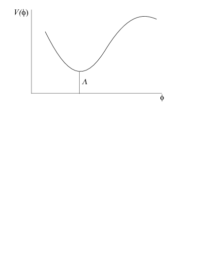
Figure 1: Potential with a local minimum and a positive cosmological constant

The embedding of such a scenario in a string theory cosmological framework is one of the key challenges today (see [3] for a review). String compactifications are characterised by the appearance of a large number of moduli fields  and the question is whether some of these moduli could be appropriate inflaton candidates.

In string compactifications the ten-dimensional space-time is assumed to be a direct product of the four-dimensional Minkowski spacetime and a six-dimensional Calabi-Yau (CY) manifold characterised by a compact ‘radius’ $R$. The classical supergravity equations, however, remain invariant under rescalings of the size $R$ of the compact manifold. Consequently, for any solution which determines four dimensional effective theory models such as the Standard Model, we encounter a family of solutions by just changing the parameter $R$. In fact, from the four-dimensional theory point of view, $R$ corresponds to a massless scalar field.

In general, deformations of the compactification in four dimensions correspond to massless scalars which do not acquire tree-level potential and do not affect the four-dimensional action. Such scalars are the dilaton field, the Kähler and complex structure moduli, those corresponding to brane deformations etc. The appearance of such massless scalars in the effective theory have singificant consequences. If they couple gravitationally to matter fields, they could mediate long range forces which have not been observed. They also affect the big-bang nucleosynthesis and have implications on the cosmological evolution. Therefore, to construct a realistic effective field theory model, it is important to generate a potential with de Sitter vacuum and assure a positive mass-squared for the various moduli at large enough volume to allow perturbative calculation. This is dubbed as the “moduli stabilisation” problem.

Because there are a large number of choices of CY manifolds and quantised fluxes which determine the properties of the effective field theory and, particularly, the scalar potential, string theory is characterised by a vast number of vacua, which constitute the so called “string landscape”. However, whether there exist any de Sitter vacua amongst the plethora of possibilities is a long standing issue and the subject of an ongoing debate today. The string computational tools used to determine their existence are mainly the various moduli fields, the Kähler potential and the flux-induced superpotential in the effective field theory limit obtained after compactification. Since the tree-level potential for moduli fields vanishes identically, possible interesting non-zero contributions are based on $\alpha^{\prime}$ and string loop corrections as well as on non-perturbative effects. Notwithstanding the accumulated work and the variety of models that have appeared the last decades providing evidence for the existence of the desired dS vacua, most -if not all- proposed solutions are based on assumptions and ingredients that might not be supported in a fully fledged string theory construction. These doubts are corroborated by the fact that a number of no-go theorems (see for example [7, 8, 9] ) preclude the existence of dS vacua, although at the classical level and under certain assumptions that may not be universally true in string theory.

On the other hand, recently, some criteria on the (non)-existence of dS vacua in string theory have been proposed. The swampland conjecture suggested by the authors [10, 11] states that the scalar potential $V$ of any effective field theory consistent with string theory satisfies the bound

$$\frac{|\nabla V|}{V}\;\geq\;\frac{c}{M_{P}}$$ (1)

where $c$ is a positive constant of order one. This bound excludes stable or meta-stable de Sitter string vacua and, if true, it suggests that the latter belong to the swampland. In a standard inflationary scenario this essentially means that the slow-roll parameter $\epsilon$ is violated at order one.

Then, in the string framework the alternative interpretation of the present day value of the cosmological constant is through quintessence, provided the potential is positive, $V>0$, and $|\nabla V|\sim V$ (for a review in quintessence see for example [12] and in the context of strings [13]). Counterexamples explaining how the bound  (1) could be evaded have been proposed (see for example [14, 15, 16, 17]. However, the authors [18] (see also [19, 20]) proposed a refined version of the conjecture, according to which the potential must satisfy either the bound (1) or the constraint associated with the minimum value of the mass spectrum:

$${\rm min}(\nabla_{i}\nabla_{j}V)\;\leq\;-\frac{c^{\prime}}{M^{2}_{P}}$$ (2)

Here, $c^{\prime}$ is a positive constant of order one. The two bounds together, still forbid de Sitter minima but allow the existence of maxima.

In the ensuing years after the experimental confirmation of the accelarating expansion of the universe, there has been a lot of activity to construct effective theories of string origin with de Sitter vacua. However, the moduli space and the induced action used to determine the four-dimensional vacua are not exactly known and the proposed models are based on assumptions regarding the significance of the various quantum corrections. Focusing on type IIB effective string theories in particular, the usual procedure in obtaining vacua is based on flux compactifications with $\alpha^{\prime}$ and loop corrections playing a central rôle in moduli stabilisation. However, two of the most questioned ingredients introduced are the non-perturbative corrections in the superpotential and the uplifting term (to ensure a dS vacuum) obtained from anti-$D3$ ($\overline{D3}$) branes.

The focus of this talk is on this issue. That is, to examine alternative solutions to the problems of moduli stabilisation and to consolidate a de Sitter vacuum based only on perturbative corrections. The layout of the talk is organised as follows. It will start with a short presentation of the string derived no-scale effective supergravity mainly focusing on the description of the moduli space, the flux induced superpotential and the Kähler potential in the context of type IIB theory. Next, a short description of the rôle of non perturbative effects on moduli stabilisation will be given and two familiar models proposed some 15 years ago will be briefly outlined. Afterwards, a new solution to the problem of moduli stabilisation based only on perturbative corrections in the presence of 7-branes will be presented in some detail. The presentation will resume with a brief exposition of the cosmological implications of this model. More precisely it will be shown that, in the presence of a new Fayet-Iliopoulos term, the slow-roll inflation scenario can also be realised.

2 The general type IIB set up

In this talk we will discuss the issues of moduli stabilisation, de Sitter vacua and inflation in a type IIB/F-theory framework  . We will start with a presentation of the basic elements used to obtain the scalar potential of the effective $4d$ field theory, concentrating on the bosonic spectrum and the moduli space. The type IIB spectrum is obtained by combining left and right moving sectors with Neveu-Schwarz (NS) and Ramond (R) boundary conditions. The bosonic spectrum includes the graviton $g_{\mu\nu}$, a scalar $\phi$ (the dilaton), the two-index antisymmetric tensor $B_{\mu\nu}$-the so called Kalb-Ramond (KB) field, and the $p$-form potentials $C_{p},p=0,2,4$. The axion and the dilaton fields are combined to form the axion-dilaton

$$S=C_{0}+ie^{-\phi}$$ (3)

In addition, various other geometric moduli corresponding to the deformations of the metric $g_{\mu\nu}$ emerge which are related to the shape, size and other properties of the compactification manifold. In particlular, these are classified as follows:

1. Kähler moduli $T^{a}$ corresponding to deformations of the Kähler form $J=ig_{i\bar{j}}dz^{i}\wedge d\bar{z}^{\bar{j}}\to T^{a}\omega_{a}$, where $\omega_{a},\,a=1,2,\dots,h^{1,1}$ is a basis for harmonic (1,1)-forms.

2. Complex Structure moduli $z^{b},\;b=1,2,\dots,h^{2,1}$ being harmonic (2,1)-forms, corresponding to deformations associated with a (3,0)-form, denoted with the greek letter $\Omega$. Clearly, the latter depends on the complex structure moduli $\Omega=\Omega(z_{a})$

3. Scalar fields $b^{a},c^{a},\vartheta^{a}$ arising from the expansion of the $B_{2},C_{2},C_{4}$ potentials in the appropriate basis of harmonic forms.

4. Moduli associated with $D7$ brane deformations, $D3$ positions etc.

In order to describe the four dimensional effective supergravity limit of type IIB string, we need to derive the superpotential and the Kähler potential.

In type IIB string theory the superpotential is generated by 3-form fluxes which are constructed from the KB-field and the $C_{p}$ potentials. The latter give rise to the field strengths

$$F_{p}:=d\,C_{p-1},\;H_{3}:=d\,B_{2}~{},$$ (4)

From these, the following combination is assumed

$$G_{3}:=F_{3}-S\,H_{3}~{},$$ (5)

where $S$ is given in (3). Using the holomorphic (3,0)-$\Omega$ form, the flux induced superpotential is

$${\cal W}_{0}=\int G_{3}\wedge\Omega(z_{a})~{},$$ (6)

while $G_{3}$ should be primitive $(2,1)$ form to allow ${\cal N}=1$ supersymmetry. The superpotential (6) depends on the compex structure moduli $z_{a}$ through its $\Omega$ dependence but it does not involve the Kähler structure moduli. To ensure the flatness of the superpotential, we impose the supersymmetric conditions, setting zero the covariant derivatives with respect to the ${z_{a}}$ and $S$ fields:

$${\cal D}_{z_{a}}{\cal W}_{0}=0,\;{\cal D}_{S}{\cal W}_{0}=0~{}.$$ (7)

The solutions of these equations stabilise the complex structure moduli and the axion dilaton field. Both are assumed to obtain masses of the order of the string scale, while ${\cal W}_{0}$ becomes a constant. However, because the Kähler moduli do not participate in ${\cal W}_{0}$, at this stage, they remain completely undetermined.

Next we proceed with the second significant ingredient of the theory, namely the Kähler potential. Ignoring for the moment any quantum corrections, the classical Kähler potential ${\cal K}$ is given by the formula

$${\cal K} = -\sum_{i=1}^{3}\ln(-i({T_{i}-\bar{T_{i}}}))$$ (8)

$$-\ln(-i({S-\bar{S}}))-\ln(i\int{\Omega}\wedge{\bar{\Omega}})~{}\cdot$$

In (8) we have assumed the contribution of three Kähler moduli fields, $T_{i},\,i=1,2,3$ and $S$ is the axion-dilaton defined in (3). Moreover, ${\Omega}={\Omega}(z_{a})$ , is the holomorphic (3,0)-form [24], already introduced previously, whilst ${\bar{\Omega}}$ stands for its corresponding antiholomorphic one.

From (8), we can compute the scalar potential, using the standard supergravity formula

$${V} = e^{\cal K}(\sum_{I,J}{\cal D}_{I}{\cal W}_{0}{\cal K}^{I\bar{J}}{\cal D}_{\bar{J}}{\cal W}_{0}-3|{\cal W}_{0}|^{2})$$ (9)

The sum is under all moduli fields, ($z_{a},T_{i},S$), while ${\cal K}_{I\bar{J}}=\partial_{I}\partial_{\bar{J}}{\cal K}$ and ${\cal K}^{I\bar{J}}$ its inverse. Due to no-scale structure, at the classical level, this is identically zero and this can be easily seen by splitting the sum into that of the Kähler moduli and the rest moduli fields:

$${V} = e^{\cal K}\sum_{I,J=z_{a},S{\neq T_{i}}}D_{I}{\cal W}_{0}{\cal K}^{I\bar{J}}D_{\bar{J}}{\cal W}_{0}\;\;({D_{I}{\cal W}_{0}=0},\,{\rm flatness})$$

$$+e^{\cal K}\left(\sum_{I,J=T_{i}}{\cal{K}}_{0}^{I\overline{J}}\partial_{I}{\cal W}_{0}\partial_{\overline{J}}{\cal W}_{0}-3|{\cal W}_{0}|^{2}\right)\;\;({=0},\;{\rm no\,scale})$$

$$= 0$$

The first line is zero due to supersymmetric conditions (7) which fix the scalars $z_{a},S$ while the second line vanishes identically in no-scale models. Hence, at this level a scalar potential with zero vacuum energry is obtained and the Kähler moduli remain unfixed.

3 Non Perturbative Corrections

Up to this point we have seen that it is not possible to stabilise all moduli and construct a potential with dS minimum at the classical level. To circumvent this problem, most of the suggested solutions rely on non-perturbative corrections to the superpotential . (Recall that perturative corrections in ${\cal W}_{0}$ are not allowed because of non-renormalisation theorems.) For the sake of completeness of the presentation, two representative solutions will be briefly sketched, namely, ${\cal A}$) the KKLT model and ${\cal B}$) the large volume scenario (LVS).

Case ${\cal A}$:  In the simplest version of the model [25], one assumes corrections of the form

$${\cal W}={\cal W}_{0}+Ae^{-\lambda T}$$ (10)

A possible origin of these corrections come from a stack of $N$ 7-branes, wrapping 4-cycles, and it is associated with ${\cal N}=1$ supersymmetric $SU(N)$ symmetry. In this case gaugino condensation can take place and the constant $\lambda$ is given by $\lambda=2\pi/{N}$, for $SU(N)$. This way, the supersymmetric condition ${\cal D}_{T}{\cal W}=0$ stabilises the $T$-modulus, however, this solution requires unnatural fine-tuning of the parameters ${\cal W}_{0},\,A$ and ${\lambda}$. Moreover, the so obtained vacuum has an AdS (supersymmetric) minimum

$${V_{AdS}}\propto-3|{\cal W}|^{2}e^{\cal K}\,{<}\,0~{},$$ (11)

in obvious conflict with the cosmological observations which imply $\Lambda>0$.

A solution to this problem is obtained by uplifting the vacuum to a ${\bf dS}$ minimum with the inclusion of a positive contribution $V_{\overline{D3}}$ coming from ${\overline{D3}}$ branes, so that the total contribution equals the cosmological constant

$$V_{\overline{D3}}-|V_{AdS}|\approx 10^{-120}M_{P}^{4}$$ (12)

The $\overline{D3}$’s source of positive energy comes from ${\overline{D3}}\,$ tension and the 3-form fluxes are introduced to cancel the Tadpole. Indeed, for $N_{3}(\bar{N}_{3})$ number of $D3(\overline{D3})$ branes the charge $Q_{3}=N_{3}-\bar{N}_{3}$ is determined by the global tadpole condition

$$\frac{\chi{(X)}}{24} = Q_{3}+\frac{1}{2\kappa^{2}_{10}{\cal T}_{3}}\int H_{3}\wedge F_{3}~{},$$ (13)

where, in an F-theory framework, ${\chi{(X)}}$ is the Euler characteristic of the CY fourfold $X=CY_{4}$, and ${\cal T}_{3}$ is the tension of the $D3$-brane. Now, according to Klebanov-Strassler’s description [26], charge conservation is imposed by assuming appropriate $M$ and $-K$ units of charge $\int_{A}F_{3}=4\pi^{2}M,\;\int_{B}H_{3}=-4\pi^{2}K$, where the integrals are over the $A$-cycle and its dual $B$-cycle respectively. In addition, the fluxes generate a superpotential for the complex structure moduli [27]. The positive energy of the $\overline{D3}$ depends on the warp factor $e^{A}$:

$$V_{\overline{D3}}=2{\mu}e^{4A},\;\;ds_{10}^{2}=e^{2A}dx_{4}^{2}+e^{-2A}dy_{6}^{2}~{}.$$

However, as pointed out in the above references (see [27, 28]), the supersymmetry preserved by the $\overline{D3}$ branes is incompatible with the global supersymmetry preserved by the imaginary self-dual 3-form flux of the background geometry and as a result, this configuration is unstable.

Another way to parameterise the uplifting of an AdS vacuum of the potential to a de Sitter one, is by using nilpotent chiral multiplets. In this version of the KKLT construction a goldstino multiplet $S_{NL}=s+\sqrt{2}\theta G+\theta^{2}F_{S}$ satisfying the constraint $S_{NL}^{2}=0$ associated with non-linearly realised supersymmetry of the Volkov-Akulov type is introduced . In this framework, the superpotential and the Kähler potential are [29, 30]

$${\cal W} = {\cal W}_{0}+A\,e^{-\lambda T}+\mu^{2}S_{NL}$$ (14)

$${\cal K} = -3\,\ln(T-\bar{T})+S_{NL}\bar{S}_{NL}$$ (15)

where, as above, $T$ is the Kähler modulus associated with the volume and $S_{NL}$ the nilpotent goldstino superfield $S_{NL}^{2}=0$. Computing the scalar potential, one finds 

$$V_{\rm new}=V_{AdS}+V_{up}=V_{AdS}+\frac{\mu^{4}}{(T+\bar{T})^{3}}$$ (16)

Therefore, the existence of a nilpotent goldstino implies an uplifting term exactly as the one obtained by the $\overline{D3}$ brane. The important difference is that now this is manifestly supersymmetric. However, given the doubts whether these features can be part of a realistic string scenario and the amount of fine-tuning required, the importance of these effects on the determination of a true de Sitter vacuum remains distinctly nebulous.

Case ${\cal B}$: The Large Volume Scenario (LVS) [34] can be thought as a generalisation of the above constructions, aiming to improve some of the aforementioned deficiencies. This proposal is also based on the assumption of non-perturbative corrections to the superpotential but it is realised with an exponentially large volume. In the simplest version the volume is given by ${\cal V}=\tau_{b}^{3/2}-\tau_{s}^{3/2}$ where $\tau_{b},\tau_{s}$, ( for a generalisation see [35]) are two distinct Kähler moduli. The superpotential and Kähler potential are given by

$$\mathcal{W}_{LVS} =\mathcal{W}_{0}+A\,e^{-\lambda\tau_{s}}~{},$$ (17)

$$\mathcal{K}_{LVS} =-2\textrm{ln}(\tau_{b}^{\frac{3}{2}}-\tau_{s}^{\frac{3}{2}}+\xi)~{}.$$ (18)

The new ingredient in the Kähler potential is a constant $\xi$ which arised due to $\alpha^{\prime}$ corrections, and it is proportional to the Euler number [36]

$$\xi=-\frac{\zeta(3)}{4(2\pi)^{3}}\chi$$ (19)

Both, gaugino condensation and the $\alpha^{\prime}$ correction $\xi$ are required to stabilise the Kähler moduli ${\tau_{b}},{\tau_{s}}$. However, as in KKLT scenario (case ${\cal A}$), a mechanism is required to uplift the potential to a dS minimum. This can be done by introducing gauge field fluxes on $D7$-branes which induce a D-term potential in the effective four dimensional model [37].

4 Perturbative moduli stabilisation

In the rest of this talk, an alternative scenario of Kähler moduli stabilisation will be presented which does not rely on any uncontrolable non-perturbative terms in the superpotential. Earlier computations [38, 39] focused on one-loop corrections in the string coupling and contributions to order ${\alpha^{\prime}}^{3}$ [40] breaking the no-scale invariance of the Kähler potential. However, it was realised that these are not capable of stabilising the volume and the Kähler moduli $T_{i}$ in general, unless a $T_{i}$-dependent superpotential is assumed. Instead, the proposed mechanism can be realised in a type IIB/F-theory framework and relies on the presence of logarithmic corrections induced by $D7$-branes [41] in the 4d effective action. At the end of this talk it will be shown how the incorporation of a new Fayet-Iliopoulos (FI)-term [42] will allow for a slow-roll inflation.

To be more specific, a geometric configuration of three intersecting 7-branes with fluxes will be considered with the corresponding Kähler moduli fields denoted as $T_{a}=\tau_{a}+ib_{a}$. We begin with the description of the basic ingredients. It is known that when ${\cal O}({\alpha^{\prime}}^{3})$ corrections are taken into account, the definition of the four-dimensional dilaton $\phi_{4}$, in terms of the ten-dimensional one, is given by

$$e^{-2\phi_{4}}=e^{-2\phi}\left({\cal V}+\xi\right)$$ (20)

where ${\cal V}$ is the CY volume and $\xi$ the constant (19) which is proportional to the Euler number. To express the volume in terms of the Kähler moduli we introduce the following notation:
We denote with $v^{a}$ the 2-cycle volume modulus transverse to the $D7_{a}$ brane and, assuming three intersecting branes, the total volume is given by

$${\cal V}=\frac{1}{6}\kappa_{abc}v^{a}v^{b}v^{c}~{},$$ (21)

where $\kappa_{abc}$ are intersection numbers. The world volume associated with the $D7$ brane is defined by

$$\tau_{a}=\frac{1}{6}\kappa_{abc}v^{b}v^{c}~{},$$ (22)

Taking into account the ${\alpha^{\prime}}^{3}$ corrections in type IIB, the Kähler potential is given by the formula

$${\cal K}=-2\ln(e^{-2\phi}({\cal V}+\xi))-\ln\left(\int\Omega\wedge\bar{\Omega}\right)+{\rm constant}$$ (23)

In order to convert (20) in the Einstein frame, we define

$$\hat{v}_{a}=v_{a}e^{-\phi/2}=\frac{\tau_{a}}{g_{s}^{1/2}},\;\;\hat{\xi}=\xi e^{3\phi/2}={\xi}{g_{s}^{3/2}}~{}.$$ (24)

Then, in terms of (24), expression (20) is written

$$e^{-2\phi_{4}}=e^{-\frac{1}{2}\phi}\left(\hat{\cal V}+\hat{\xi}\right)~{},$$

where $\hat{\cal V}=\frac{1}{6}\kappa_{abc}\hat{v}_{a}\hat{v}_{b}\hat{v}_{c}$. Then the Kähler potential takes the form:

$${\cal K}=-\ln({S-\bar{S}})-2\ln(\hat{\cal V}+\hat{\xi})-\ln\left(\int\Omega\wedge\bar{\Omega}\right)+{\rm constant}~{},$$ (25)

where use has been made of the relation $S-\bar{S}\propto e^{-\phi}$ derived from (3).

The specific form (25) of the Kähler potential in type IIB can be confirmed by a T-duality transformation [43] from that of type IIA.

4.1 Logarithmic loop corrections and D-terms from $D7$-branes

$D7$ and $D3$ branes are essential elements in configurations aiming to describe viable effective field theories derived from type IIB flux compactifications and its F-theory geometric analogue. Their deformations are important ingredients of the moduli space and could be useful to ensure a successful inflationary scenario and a stable de Sitter vacuum. In such configurations, branes which span different dimensions of the compact space intersect each other and, depending on the details of the geometry and fluxes, may be associated with anomalous $U(1)$ symmetries. Then, the resulting chiral spectrum of the four dimensional effective theory induces Fayet-Iliopoulos D-terms in the effective potential. Based on these observations, in the following, we will examine the rôle of intersecting D7 brane configurations in moduli stabilisation, de Sitter vacua and slow roll inflation.

We start with the observation that in the large volume limit, a nonvanishing $\xi$ correction gives rise to localised graviton kinetic terms in the Calabi-Yau compact manifold at the points where the Euler number is concentrated. As discussed in [44], this implies a localised Einstein action and there is an emission of closed strings from the associated graviton vertices into the various $D$ branes of the assumed geometric configuration, giving rise to local tadpoles. In the case of $D7$ branes, closed strings propagating in the the two-dimensional transverse space induce an infrared divergence which exhibits a logarithmic dependence in the regime of large transverse volume of codimension two [41]. Due to the infrared divergence, one could also expect that it is the dominant correction at that order in the string loop expansion. For the simplest case of a single $D7$ brane, denoting the size of the transverse dimensions with $u$, the corresponding loop correction takes the form

$$\delta=\gamma\ln(u)~{},$$ (26)

where $\gamma$ is a model dependent parameter. These corrections, together with the ${\alpha}^{\prime}$ corrections discussed earlier, appear in Einstein kinetic terms in ${\cal S}$:

$${\cal S}=-\frac{1}{2\kappa^{2}_{4}}\,\int d^{4}x\sqrt{-g}\left(e^{-2{\phi}}({\cal V}+{\xi})+{\delta}\right){{\cal R}}+\cdots$$

The Kähler potential takes the form [43]

$${\cal K}=-\ln({S-\bar{S}})-2\ln(\hat{\cal V}+\hat{\xi}+\hat{\delta})-\ln\left(\int\Omega\wedge\bar{\Omega}\right)+{\rm constant}~{},$$ (27)

where $\hat{\delta}=\delta g_{s}^{1/2}$. One can notice that both $\xi$ and $\delta$ corrections break the no-scale form of the Kähler potential.

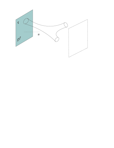
Figure 2: Sting loops from exchange of closed strings between graviton vertices and $D7$-branes when $\xi\neq 0$.

Next, we describe the second important effect of the $D7$ branes which are associated with anomalous $U(1)$ symmetries. As already mentioned, there is an induced D-term which has the generic form dictated by the effective ${\cal N}=1$ supergravity [37, 45, 46, 47]:

$$V_{D}=\frac{g_{D7}^{2}}{2}\left(iQ\partial_{T^{a}}{\cal K}(T^{a})+\sum_{J}Q_{J}\mid\langle\phi^{J}\rangle\mid^{2}\right)^{2}$$ (28)

The gauge coupling is fixed by the kinetic function: $\frac{1}{g^{2}_{D7}}={\rm Im}(T^{a})$ and $\phi^{J}$ are scalar components of superfields whose charges $Q_{J}$ are subject to anomaly cancellation conditions, which are automatically satisfied in a consistent string background [48, 49]. Although in general the VEVs of the scalar fields may be non-zero, for our present purposes we can ignore the matter fields and write (28) as follows

$$V_{D}=-\frac{d_{a}}{{2\rm Im}(T^{a})}\left(\partial_{T^{a}}{\cal K}(T^{a})\right)^{2},$$ (29)

in which $d_{a}=Q^{2}$.

Before we start a detailed analysis of the model, it is important to set out the basic features required for an acceptable dS vacuum. We have seen that at the classical level the effective potential vanishes due to no-scale properties and flatness conditions. The inclusion of perturbative moduli-dependent quantum corrections in the Kähler potential should induce contributions to the scalar potential, $V(t)$ with $t=(\tau,u)$. The validity of perturbation theory implies that such corrections should vanish for $t\to\infty$ and therefore $\lim_{t\to\infty}V(t)\to 0$. If the zero at infinity is reached from negative values, then, for reasonable potentials, this implies an AdS minimum which is not acceptable. Thus, the vanishing of the potetnial at infinity should be approached from positive values. Again, for non-contrived structures of the potentials , this implies that there should be somewhere a maximum before a dS minimum is formed. This is plotted in figure  3.

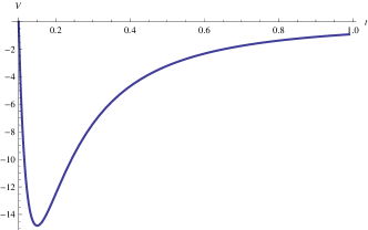
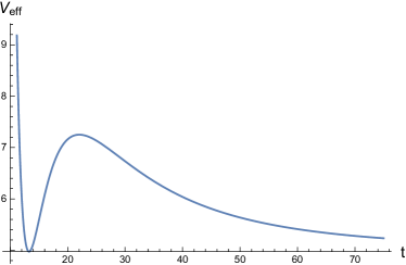
Figure 3: Anticipated shapes of the scalar potential including moduli-dependent perturbative corrections plotted vs the modulus $t$.  Left: a typical potential with AdS minimum. Right: Imposing the condition $\lim_{t\to\infty}V(t)\to 0$ and the requirement of de Sitter minimum, imply also a maximum at some finite $t$.

4.2 $D7$ Branes and Moduli Stabilisation

Having determined the form of the perturbative quantum corrections arising in the presence of ${D7}$ branes, we can investigate their rôle in the effective theory. It can be shown [43] that the stabilisation of the Kähler moduli requires at least three magnetised 7 branes intersecting each other. Therefore, we consider here directly the effects of three $D7$ branes. We introduce three Kähler moduli $T_{1},T_{2},T_{3}$ and express the internal 6d volume in terms of their imaginary parts $\tau_{k}=\frac{1}{2i}(T_{k}-\bar{T}_{k})$. We first recall that the volume is given by (21). Given also the relation (22), we can write

$${\cal V}=(\tau_{1}\tau_{2}\tau_{3})^{\frac{1}{2}}~{}\cdot$$ (30)

In terms of (30), the Kähler potential is written as follows

$${\cal K} = -2\ln\left((\tau_{1}\tau_{2}\tau_{3})^{\frac{1}{2}}+\xi+\sum_{k=1}^{3}\gamma_{k}\ln(\tau_{k})\right)~{},$$ (31)

where $\gamma_{k}$ are model dependent coefficients of order one. For simplicity we take $\gamma_{1}=\gamma_{2}=\gamma_{3}\equiv\gamma_{\tau}$, and absorb the $\alpha^{\prime}$ corrections, $\xi$, into the logarithmic term by a new parameter $\mu=e^{\frac{\xi}{2\gamma_{\tau}}}$ so that

$$\xi+2\gamma_{\tau}\ln({\cal V})=2\gamma_{\tau}\ln(\mu{\cal V})~{}.$$ (32)

The F-term potential is

$$V_{F}=3\gamma_{\tau}W_{0}^{2}\frac{\ 2(\gamma_{\tau}+2{\cal V})+(4\gamma_{\tau}-{\cal V})\ln(\mu{\cal V})}{({\cal V}+2\gamma_{\tau}\ln(\mu{\cal V}))^{2}\left(6\gamma_{\tau}^{2}+{\cal V}^{2}+8\gamma_{\tau}{\cal V}+\gamma_{\tau}(4\gamma_{\tau}-{\cal V})\ln(\mu{\cal V})\right)}~{},$$ (33)

and in the large volume limit with small logarithmic corrections, can be approximated by

$$V_{F}\approx 3W_{0}^{2}\,\gamma_{\tau}\,\frac{\ln(\mu{\cal V})-4}{{\cal V}^{3}}~{}\cdot$$ (34)

D-term contributions to the effective potential in the presence of $D7$ fluxed branes take the form

$$V_{D} = \sum_{a=1}^{3}\frac{d_{a}}{\tau_{a}}\left(\frac{\partial{\cal K}}{\partial\tau_{a}}\right)^{2}\approx\sum_{a=1}^{3}\frac{d_{a}}{\tau_{a}^{3}}~{},$$ (35)

where the approximation holds in the large volume limit.

Hence, when both, F- and D-term contributions are taken into account, in the large volume expansion, the effective potential is as follows

$$V_{\rm eff}\;\approx\;3W_{0}^{2}\,\gamma_{\tau}\,\frac{\ln(\mu{\cal V})-4}{{\cal V}^{3}}\,+\,\frac{d_{i}}{\tau_{i}^{3}}\,+\,\frac{d_{j}}{\tau_{j}^{3}}\,+\,\frac{d_{k}(\tau_{i}\tau_{j})^{3}}{{\cal V}^{6}},$$

for $i\neq j\neq k\neq i$. There are three independent variables $\tau_{1,2,3}$ and the product of them is related to the 6d-volume. We replace one of the $\tau_{i}$’s with the total volume ${\cal V}$ and minimise the potential with respect to ${\cal V}$ and the two remaining Kähler moduli. Two minimisation conditions determine the ratios between the moduli, $\left(\frac{\tau_{i}}{\tau_{j}}\right)^{3}=\frac{d_{i}}{d_{j}}$ and the third one the total volume. Expressed in terms of the stabilised total volume ${\cal V}$, the conditions for the two $\tau_{i}$ can be written as

$$\tau_{i}^{3}=\left(\frac{d_{i}^{2}}{d_{k}d_{j}}\right)^{\frac{1}{3}}{\cal V}^{2}~{}\cdot$$

The minimisation condition for the total volume reads:

$$\frac{13}{3}-\ln{\cal V}\;=\;\frac{2}{3}\frac{d}{\gamma}\,{\cal V}~{}.$$ (36)

Inserting the three conditions in $V_{\rm eff}$ we obtain the simple form

$$V_{\rm eff}\approx\gamma\,\frac{\ln(\mu{\cal V})-4}{{\cal V}^{3}}+\frac{d}{{\cal V}^{2}}~{},$$ (37)

with

$$d=3(d_{1}d_{2}d_{3})^{\frac{1}{3}}~{}\;;\;\gamma=3W_{0}^{2}\gamma_{\tau}~{}\cdot$$ (38)

The above scalar potential possesses a dS minimum in some region of the parameter space [43]. To show this, we introduce the convenient definition:

$${w} = \frac{13}{3}-\ln{\cal V}~{}.$$ (39)

Then, vanishing of the derivative of the potential with respect to ${\cal V}$ (i.e. condition 36), takes the form:

$$we^{{w}}\;{=}\;{z}~{}.$$ (40)

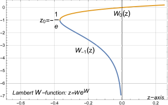
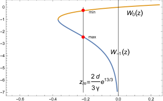
Figure 4: Left: The two branches of the Lambert $W$-function, $W_{0}$ and $W_{-1}$, respectively. Right: The two values of the world volume ${\cal V}$ for fixed $d/gamma$ ratio, corresponding to the minimum and the maximum of the scalar potential.

where, in the present case the variable $z$ is related to the ratio of the two constants,

$${z}=\frac{2}{3}\frac{d}{\gamma}e^{\frac{13}{3}}~{}.$$ (41)

Inversion of (40) determines ${w}$ and consequently ${\cal V}$ through (39). The final solution given by multivalued Lambert $W$-function [50]

$$w\Rightarrow{W}({z})~{}.$$ (42)

The two branches of the Lambert function ${W_{0}}({z})$ and ${W_{-1}}({z})$ are shown in figure 4. Real values of ${W_{0}},{W_{-1}}$ are obtained for ${z}\geq{z_{0}}=-{e}^{-1}$.

Furthermore, the values of the parameters $d$ and $\gamma$, whose ratio determines $z$, must be such that the scalar potential $V=V({\cal V})$ has a minimum and a maximum w.r.t. the volume ${\cal V}$, or equivalently w.r.t. to the function $W(z)$ as can be inferred from their relation, see (39) and (42). Thus, we are interested for solutions such that $z$ (determined from the ratio of parameters $d$ and $\gamma$, see Eq (41)), falls in the range where, simultaneoulsy two solutions for the volume can be obtained. In the right hand side of figure 4 the vertical line represents any value of ${z_{m}}=\frac{2{d}}{3{\gamma}}e^{\frac{13}{3}}$ between

$$-{e}^{-1}\leq\frac{2{d}}{3{\gamma}}e^{\frac{13}{3}}\leq 0~{},$$ (43)

where $V_{min}$ and $V_{max}$ can coexist. The maximum of the scalar potential corresponds to the intersection of the $z_{m}$ line with the branch $W_{-1}(z_{m})$ whilst the minimum is determined by the intersection of $z_{m}$ with $W_{0}(z_{m})$.

The requirement for de Sitter vacua puts additional restrictions. To implement this constraint, we first compute the minimum value of the scalar potential. The volume at the minimum is

$${\cal V}_{0}=e^{\frac{13}{3}-{W_{0}}(\frac{2}{3}\frac{d}{\gamma}e^{\frac{13}{3}})}$$

We substitute ${\cal V}_{0}$ in ${V_{\rm eff}=V_{F}+V_{D}}$ and require $V_{\rm eff}$ to be positive:

$${V_{\rm eff}^{min}}=\frac{\gamma}{{\cal V}_{0}^{3}}+\frac{d}{{\cal V}_{0}^{2}}>0$$

This constraint puts an upped bound on the ratio $\frac{d}{\gamma}$. Combined with the lower bound on $z$ in (43), we obtain the range

$$-7.242<10^{3}\frac{d}{\gamma}<-6.738~{}\cdot$$ (44)

5 Slow roll inflation

As is well known, slow-roll inflation occurs by a scalar field $\phi$, dubbed the inflaton, which starts from the top of the potential $V(\phi)$ rolling down slowly compared to the expansion of the Universe. The equation of motion is

$$\ddot{\phi}+3H\dot{\phi}+V^{\prime}(\phi)=0\,,$$ (45)

where the derivative $V^{\prime}$ is w.r.t $\phi$. The expansion of the universe $H=\frac{\dot{a}}{a}$ is involved in the friction term and its derivative implies $\frac{\ddot{a}}{a}=\dot{H}+H^{2}=H^{2}(1-\varepsilon)$, where $\varepsilon=-\frac{\dot{H}}{H^{2}}$ is one of the slow roll parameters. In order to have accelarated expansion, $\ddot{a}>0$, this must be bounded in the region $0<\varepsilon<1$. Furthermore, to ensure slow rolling with almost constant velocity of the inflaton along the potential, a second condition should be imposed: $\ddot{\phi}\ll|H\dot{\phi}|$. This is associated with a second slow roll parameter $\eta=-\frac{\ddot{\phi}}{H\dot{\phi}}<1$. Under the above conditions the equation of motion (45) can be approximated $3H\dot{\phi}\approx-V^{\prime}(\phi)$.

To study cosmological inflation in the present model, we are led to identify the inflaton field with the compactification volume modulus ${\cal V}$. To this end, in order to obtain a canonically normalised kinetic term, we perform a suitable transformation of the Kähler moduli fields. It turns out that the appropriate transformation is [51]

$$t_{i}=\frac{1}{\sqrt{2}}\ln(\tau_{i})~{},$$ (46)

Next, we switch to the normalised real scalar fields and define a convenient basis in terms of the normalised volume $t$ :

$$t = \frac{1}{\sqrt{3}}(t_{1}+t_{2}+t_{3})=\frac{\sqrt{6}}{3}\ln({\cal V})~{},$$ (47)

and two perpendicular directions

$$u = \frac{1}{\sqrt{2}}(t_{1}-t_{2})~{},$$ (48)

$$v = \frac{1}{\sqrt{6}}(t_{1}+t_{2}-2t_{3})~{}\cdot$$ (49)

In order to have a model consistent with an effective theory with positive cosmological constant, we would like to accommodate the slow-roll inflation and at the same time to ensure a dS vacuum. However, although a dS minimum exists, the actual allowed region of the parameter space is too restrictive, see Fig. 5, and additional requirements for slow-roll inflation such as the number of efoldings are hard to be met.

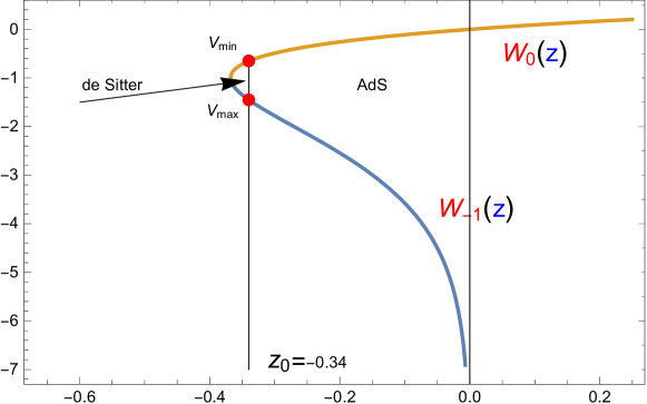
Figure 5: The allowed region for a dS minimum. The vertical line $z_{0}=-0.34$ defines the maximum ‘distance’ of the two extrema of the scalar potential $V_{F}+V_{D}$ consistent with a dS vacuum.

Therefore, in the context of the present construction, the implementation of the inflationary scenario would not be possible unless a suitable uplifting term is included in the scalar potential [51].

A possible way out of this impasse is a novel Fayet-Iliopoulos (FI)-term proposed in  [52]. This term is gauge invariant at the Lagrangian level and can be written for a non-R $U(1)$ symmetry [53]. With this in mind, we introduce a constant term $V_{up}$ associated to a $U(1)$ of a $D3$-brane, so that the effective potential takes the form [51]:

$$V_{\rm eff} = \gamma\,\frac{1}{2}e^{-\frac{3\sqrt{6}}{2}t}(\sqrt{6}t-8)+d\,e^{-\sqrt{6}t}+V_{up}~{},$$ (50)

with the modulus $t$ related to the total volume via (47) and $\gamma$ defined in eq. (38).

Inflation should occur in an interval $t=(t_{end},t_{*})$ which lies between the maximum and the minimum of the scalar potential. The first end of the interval is the ending point of inflation, which corresponds to the breaking of the slow-roll condition:

$$t_{end}={\rm max}\left[t|_{\frac{1}{2}\left(\frac{V^{\prime}}{V}\right)^{2}\simeq 1},t|_{\frac{|V^{\prime\prime}|}{V}\simeq 1}\right],$$ (51)

where the derivatives $V^{\prime},V^{\prime\prime}$ are taken with respect to $t$. The second point is the one corresponding to the anticipated number of e-foldings $N_{*}\sim 50$ to 60, where $N_{*}$ is given by the formula

$$N_{*}=\int_{t_{end}}^{t_{*}}\frac{V}{V^{\prime}}dt~{}\cdot$$ (52)

In addition, at the same point $t_{*}(N_{*})$, the spectral index should satisfy the values from observations

$$n_{s}=1-6\epsilon+2\eta=1-3\left.\left(\frac{V^{\prime}}{V}\right)^{2}\right|_{t_{*}}+2\left.\frac{V^{\prime\prime}}{V}\right|_{t_{*}}~{}\cdot$$ (53)

In Fig. 6, the case for $N_{*}=60$ efoldings is shown. As required, the region $(t_{*},t_{end})$ where infaltion takes place is stretched out between the maximum and the minimum of the potential. Because of the presence of two other scalar fields (48, 49), multi-field effects should be considered in the region where the inflaton field is no longer the lightest scalar (see [51] for a detailed analysis).

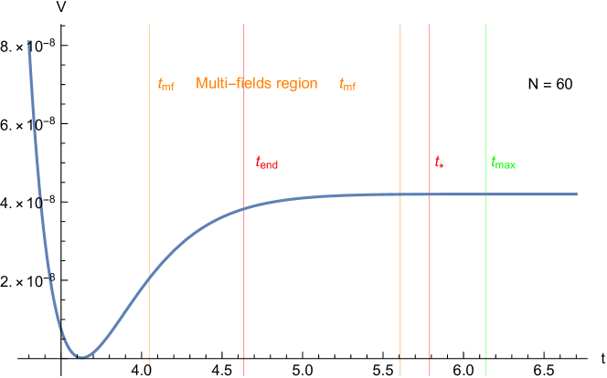
Figure 6: The scalar potential for $n_{s}=0.9605,N_{*}=60$. Inflation occurs in the region $(t_{*},t_{end})$ which lies between the maximum and the minimum of the potential. The region on the right of this line is characterised by AdS minima.

6 Conclusions

The quest for the existence of de Sitter string vacua in string theory is a fascinating subject of intensive recent reseach. Contradictory conjectures with greater or lesser theoretical foundation regarding their existence abound, and the results are far from being conclusive. Moduli fields which are always present in Calabi-Yau compactifications, play an instrumental rôle in the determination of the effective theory’s vacuum.

In this presentation an effective model in a type IIB framework is considered based on a geometric configuration with three intersecting stacks of $D7$-branes. In this set up, perturbative string loop contributions induce terms in the Kähler potential which depend logarithmically on the volume moduli associated with the directions transverse to the corresponding $D7$-branes. In this framework, the Kähler moduli fields are stabilised and a de Sitter vacuum is accommodated naturally. In the final part of this presentation, the implications on inflation are discussed.

References

- [1] A. G. Riess et al. [Supernova Search Team], Astron. J. 116 (1998) 1009 [astro-ph/9805201].
- [2] S. Perlmutter et al. [Supernova Cosmology Project Collaboration], Astrophys. J. 517 (1999) 565 [astro-ph/9812133].
- [3] D. Baumann and L. McAllister, arXiv:1404.2601 [hep-th].
- [4] M. R. Douglas and S. Kachru, Rev. Mod. Phys. 79 (2007) 733 [hep-th/0610102].
- [5] R. Blumenhagen, B. Kors, D. Lust and S. Stieberger, Phys. Rept. 445 (2007) 1 [hep-th/0610327].
- [6] A. N. Schellekens, “The String Theory Landscape,” Adv. Ser. Direct. High Energy Phys. 22 (2015) 155.
- [7] J. M. Maldacena and C. Nunez, Int. J. Mod. Phys. A 16 (2001) 822 [hep-th/0007018].
- [8] L. Covi, M. Gomez-Reino, C. Gross, J. Louis, G. A. Palma and C. A. Scrucca, JHEP 0806 (2008) 057 [arXiv:0804.1073 [hep-th]].
- [9] U. H. Danielsson and T. Van Riet, Int. J. Mod. Phys. D 27 (2018) no.12, 1830007 [arXiv:1804.01120 [hep-th]].
- [10] G. Obied, H. Ooguri, L. Spodyneiko and C. Vafa, arXiv:1806.08362 [hep-th].
- [11] P. Agrawal, G. Obied, P. J. Steinhardt and C. Vafa, Phys. Lett. B 784 (2018) 271 [arXiv:1806.09718 [hep-th]].
- [12] S. Tsujikawa, Class. Quant. Grav. 30 (2013) 214003 [arXiv:1304.1961 [gr-qc]].
- [13] M. Cicoli, S. De Alwis, A. Maharana, F. Muia and F. Quevedo, Fortsch. Phys. 2018 1800079 [arXiv:1808.08967 [hep-th]].
- [14] D. Andriot, Phys. Lett. B 785 (2018) 570 [arXiv:1806.10999 [hep-th]].
- [15] A. Kehagias and A. Riotto, arXiv:1807.05445 [hep-th].
- [16] F. Denef, A. Hebecker and T. Wrase, Phys. Rev. D 98 (2018) no.8, 086004 [arXiv:1807.06581 [hep-th]].
- [17] D. Junghans, arXiv:1811.06990 [hep-th].
- [18] H. Ooguri, E. Palti, G. Shiu and C. Vafa, arXiv:1810.05506 [hep-th].
- [19] S. K. Garg and C. Krishnan, arXiv:1807.05193 [hep-th].
- [20] D. Andriot and C. Roupec, arXiv:1811.08889 [hep-th].
- [21] F. Denef, Les Houches 87 (2008) 483 [arXiv:0803.1194 [hep-th]].
-
[22]
J. J. Heckman,
Ann. Rev. Nucl. Part. Sci. 60 (2010) 237
[arXiv:1001.0577 [hep-th]].
G. K. Leontaris, PoS CORFU 2011 (2011) 095 [arXiv:1203.6277 [hep-th]].
A. Maharana and E. Palti, Int. J. Mod. Phys. A 28 (2013) 1330005 [arXiv:1212.0555 [hep-th]]. - [23] T. Weigand, arXiv:1806.01854 [hep-th]; T. Weigand, PoS TASI 2017 (2018) 016.
- [24] P. Candelas and X. C. de la Ossa, Nucl. Phys. B 342 (1990) 246.
- [25] S. Kachru, R. Kallosh, A. D. Linde and S. P. Trivedi, Phys. Rev. D 68 (2003) 046005 [hep-th/0301240].
- [26] I. R. Klebanov and M. J. Strassler, JHEP 0008 (2000) 052 [hep-th/0007191].
- [27] S. B. Giddings, S. Kachru and J. Polchinski, Phys. Rev. D 66 (2002) 106006 [hep-th/0105097].
- [28] S. Kachru, J. Pearson and H. L. Verlinde, JHEP 0206 (2002) 021 [hep-th/0112197].
- [29] R. Kallosh and A. D. Linde, JHEP 0702 (2007) 002 [hep-th/0611183].
- [30] S. Ferrara, R. Kallosh and A. Linde, JHEP 1410 (2014) 143 [arXiv:1408.4096 [hep-th]].
- [31] Z. Komargodski and N. Seiberg, JHEP 0909 (2009) 066 [arXiv:0907.2441 [hep-th]].
- [32] I. Antoniadis, E. Dudas, D. M. Ghilencea and P. Tziveloglou, Nucl. Phys. B 841 (2010) 157 [arXiv:1006.1662 [hep-ph]].
- [33] I. Antoniadis, E. Dudas, S. Ferrara and A. Sagnotti, Phys. Lett. B 733 (2014) 32 [arXiv:1403.3269 [hep-th]].
- [34] V. Balasubramanian, P. Berglund, J. P. Conlon and F. Quevedo, JHEP 0503 (2005) 007 [hep-th/0502058].
- [35] M. Cicoli, C. P. Burgess and F. Quevedo, JCAP 0903 (2009) 013 [arXiv:0808.0691 [hep-th]].
- [36] P. Candelas, X. C. De La Ossa, P. S. Green and L. Parkes, Nucl. Phys. B 359 (1991) 21 [AMS/IP Stud. Adv. Math. 9 (1998) 31].
- [37] C. P. Burgess, R. Kallosh and F. Quevedo, JHEP 0310 (2003) 056 [hep-th/0309187].
- [38] M. Berg, M. Haack and B. Kors, Phys. Rev. D 71 (2005) 026005 [hep-th/0404087].
- [39] M. Berg, M. Haack and E. Pajer, JHEP 0709 (2007) 031 [arXiv:0704.0737 [hep-th]].
- [40] K. Becker, M. Becker, M. Haack and J. Louis, JHEP 0206 (2002) 060 [hep-th/0204254].
- [41] I. Antoniadis and C. Bachas, Phys. Lett. B 450 (1999) 83 [hep-th/9812093].
- [42] P. Fayet and J. Iliopoulos, Phys. Lett. 51B (1974) 461.
- [43] I. Antoniadis, Y. Chen and G. K. Leontaris, Eur. Phys. J. C 78, no. 9, 766 (2018) [arXiv:1803.08941 [hep-th]].
- [44] I. Antoniadis, R. Minasian and P. Vanhove, Nucl. Phys. B 648 (2003) 69 [hep-th/0209030];
- [45] H. Jockers and J. Louis, Nucl. Phys. B 705, 167 (2005) [hep-th/0409098].
- [46] A. Achucarro, B. de Carlos, J. A. Casas and L. Doplicher, JHEP 0606, 014 (2006) [hep-th/0601190].
- [47] M. Haack, D. Krefl, D. Lüst, A. Van Proeyen and M. Zagermann, JHEP 0701 (2007) 078 [hep-th/0609211].
- [48] I. Antoniadis and T. Maillard, Nucl. Phys. B 716 (2005) 3 [hep-th/0412008].
- [49] I. Antoniadis, A. Kumar and T. Maillard, hep-th/0505260 and Nucl. Phys. B 767 (2007) 139 [hep-th/0610246].
- [50] Corless, R.M., Gonnet, G.H., Hare, D.E.G. et al. Adv Comput Math (1996) 5: 329.
- [51] I. Antoniadis, Y. Chen and G. K. Leontaris, “Inflation from the internal volume in type IIB/F-theory compactification,” arXiv:1810.05060 [hep-th].
- [52] N. Cribiori, F. Farakos, M. Tournoy and A. van Proeyen, JHEP 1804, 032 (2018) [arXiv:1712.08601 [hep-th]].
-
[53]
I. Antoniadis, A. Chatrabhuti, H. Isono and R. Knoops,
“Fayet-Iliopoulos terms in supergravity and D-term inflation,”
Eur. Phys. J. C 78 (2018) no.5, 366
[arXiv:1803.03817 [hep-th]].
I. Antoniadis, A. Chatrabhuti, H. Isono and R. Knoops, arXiv:1805.00852 [hep-th]. - [54] A. Achúcarro and G. A. Palma, “The string swampland constraints require multi-field inflation,” arXiv:1807.04390 [hep-th].
- [55] I. Antoniadis, J.-P. Derendinger and T. Maillard, Nucl. Phys. B 808 (2009) 53 [arXiv:0804.1738 [hep-th]].