Linear stability analysis of transient electrodeposition in charged porous media: suppression of dendritic growth by surface conduction
Abstract
We study the linear stability of transient electrodeposition in a charged random porous medium, whose pore surface charges can be of any sign, flanked by a pair of planar metal electrodes. Discretization of the linear stability problem results in a generalized eigenvalue problem for the dispersion relation that is solved numerically, which agrees well with the analytical approximation obtained from a boundary layer analysis valid at high wavenumbers. Under galvanostatic conditions in which an overlimiting current is applied, in the classical case of zero surface charges, the electric field at the cathode diverges at Sand’s time due to electrolyte depletion. The same phenomenon happens for positive charges but earlier than Sand’s time. However, negative charges allow the system to sustain an overlimiting current via surface conduction past Sand’s time, keeping the electric field bounded. Therefore, at Sand’s time, negative charges greatly reduce surface instabilities and suppress dendritic growth, while zero and positive charges magnify them. We compare theoretical predictions for overall surface stabilization with published experimental data for copper electrodeposition in cellulose nitrate membranes and demonstrate good agreement between theory and experiment. We also apply the stability analysis to how crystal grain size varies with duty cycle during pulse electroplating.
I Introduction
Linear stability analysis is routinely applied to nonlinear systems to study how the onset of instability is related to system parameters and to provide physical insights on the conditions and early dynamics of pattern formation Langer (1980); Kessler et al. (1988); Cross and Hohenberg (1993). Some examples in hydrodynamics include the Orr-Sommerfeld equation that predicts the dependence on Reynolds number of the transition from laminar flow to turbulent flow Orr (1907a, b); Sommerfeld (1908); Orszag (1971) and the electroconvective instability that causes the transition of a quasiequilibrium electric double layer to an nonequilibrium one that contains an additional extended space charge region Zaltzman and Rubinstein (2007). Here, we focus on morphological stability analysis in which linear stability analysis is used to analyze morphological instabilities of interfaces formed between different phases observed in various diverse phenomena such as electrodeposition Kessler et al. (1988); Ben-Jacob and Garik (1990); Lopez-Tomas et al. (1995); Léger et al. (1999a); Sagués et al. (2000); Rosso et al. (2003); Schwarzacher (2004); Rosso (2007), solidification Langer (1980); Kessler et al. (1988); Ben-Jacob and Garik (1990); Cross and Hohenberg (1993) and morphogenesis Turing (1952); Cross and Hohenberg (1993). Some particular examples of morphological stability analysis include the Saffman-Taylor instability (viscous fingering) Saffman and Taylor (1958); Saffman (1986); Bensimon et al. (1986); Homsy (1987), viscous fingering coupled with electrokinetic effects Mirzadeh and Bazant (2017), the Mullins-Sekerka instability of a spherical particle during diffusion-controlled or thermally controlled growth Mullins and Sekerka (1963) and of a planar interface during solidification of a dilute binary alloy Mullins and Sekerka (1964); Sekerka (1965), and control of phase separation using electro-autocatalysis or electro-autoinhibition in driven open electrochemical systems Bazant (2013, 2017).
I.1 Stability of metal electrodeposition
We focus on electrodeposition as a specific example of an electrochemical system for which morphological stability has been widely researched both theoretically and experimentally. The fundamental aspect of electrodeposition concerns the inherent instability of the governing physics while the practical aspect is about applications such as electroplating of metals and charging of metal batteries. To elucidate the physics behind electrodeposition, in liquid electrolytes, the morphologies of electrodeposits formed and their transitions for metals such as copper, zinc and silver are particularly well studied Ben-Jacob and Garik (1990); Lopez-Tomas et al. (1995); Léger et al. (1999a); Sagués et al. (2000); Rosso et al. (2003); Rosso (2007); Schneider et al. (2017). Depending on conditions such as applied current, applied voltage and electrolyte concentration, a variety of morphological patterns such as diffusion-limited aggregation (DLA) patterns Witten and Sander (1981, 1983); Meakin (1983); Vicsek (1984); Brady and Ball (1984); Matsushita et al. (1984); Ben-Jacob et al. (1985); Sawada et al. (1986); Grier et al. (1986); Trigueros et al. (1991); Erlebacher et al. (1993), dense branching morphologies (DBM) Ben-Jacob et al. (1985); Sawada et al. (1986); Grier et al. (1986); Ben-Jacob et al. (1986, 1987); Grier et al. (1987); Ben-Jacob et al. (1988); Garik et al. (1989); Trigueros et al. (1991); Fleury et al. (1991a); Erlebacher et al. (1993); Elezgaray et al. (2000); Léger et al. (2000a) and dendritic structures Ben-Jacob et al. (1983, 1984a, 1984b, 1985); Sawada et al. (1986); Grier et al. (1986); Ben-Jacob et al. (1987, 1988); Trigueros et al. (1991) have been observed. Ion concentration fields Argoul et al. (1996); Léger et al. (1997, 1998, 1999b, 2000b); Rosso et al. (2002), electroconvection Fleury et al. (1992, 1993, 1994); Rosso et al. (1994); Huth et al. (1995), gravity-induced convection (buoyancy) Rosso et al. (1994); Huth et al. (1995); Chazalviel et al. (1996) and the presence of impurities Fleury et al. (1991b, a); Kuhn and Argoul (1993, 1994a, 1994b) have also been examined to determine their significant effects on morphology. While the range of possible morphologies of electrodeposits is diverse, for electroplating of metals, it is desirable to electrodeposit layers that are as uniform and homogeneous as possible.
Electrodeposition is also a critical process in the development of rechargeable/secondary lithium metal batteries (LMBs) that use lithium metal for the negative electrode. For negative electrodes that use lithium chemistry, because lithium metal has the lowest standard reduction potential ( vs. the standard hydrogen electrode), highest theoretical specific () and volumetric () capacities, and lowest mass density () out of all possible candidates, it is the most promising choice for achieving high energy densities in LMBs Brandt (1994); Tarascon and Armand (2001); Aurbach et al. (2002); Xu (2004); Armand and Tarascon (2008); Cairns and Albertus (2010); Scrosati and Garche (2010); Etacheri et al. (2011); Xu et al. (2014); Li et al. (2014); Tu et al. (2015); Tikekar et al. (2016a); Choi and Aurbach (2016); Blomgren (2017); Lin et al. (2017a); Cheng et al. (2017); Lin et al. (2017b); Albertus et al. (2018); Lu et al. (2018). However, the charging of LMBs is equivalent to lithium electrodeposition at the negative electrode, which is an inherently unstable process that can cause the formation of dendrites that penetrate the separator and result in internal short circuits and thermal runaway during charging Brandt (1994); Tarascon and Armand (2001); Aurbach et al. (2002); Xu (2004); Armand and Tarascon (2008); Cairns and Albertus (2010); Scrosati and Garche (2010); Etacheri et al. (2011); Xu et al. (2014); Li et al. (2014); Tu et al. (2015); Tikekar et al. (2016a); Choi and Aurbach (2016); Blomgren (2017); Lin et al. (2017a); Cheng et al. (2017); Lin et al. (2017b); Albertus et al. (2018); Lu et al. (2018). This process has been especially well investigated in lithium polymer batteries that use a polymer electrolyte Brissot et al. (1998, 1999a, 1999b, 2001); Rosso et al. (2001); Teyssot et al. (2005); Rosso et al. (2006a); Stone et al. (2012). Detailed studies of various growth modes of lithium in liquid electrolytes during charging have been recently performed Bai et al. (2016); Kushima et al. (2017); Bai et al. (2018), which will aid in the development of better models for lithium electrodeposition. Modern lithium-ion batteries (LIBs) Brandt (1994); Tarascon and Armand (2001); Aurbach et al. (2002); Whittingham (2004); Xu (2004); Armand and Tarascon (2008); Bruce et al. (2008); Cairns and Albertus (2010); Scrosati and Garche (2010); Goodenough and Kim (2010); Etacheri et al. (2011); Goodenough and Park (2013); Li et al. (2014); Blomgren (2017); Lu et al. (2018) partially mitigate this problem of dendrite formation and propagation by employing lithium intercalating materials such as graphite for the negative electrode where only lithium ions and not reduced lithium atoms are involved in the intercalation reactions, which is also known as the “rocking chair technology” Tarascon and Armand (2001). Nonetheless, lithium plating still occurs in LIBs when they are charged at high rates or low temperatures Vetter et al. (2005); Goodenough and Kim (2010); Goodenough and Park (2013); Li et al. (2014); Palacín and Guibert (2016). Although the root causes of the widely publicized LIB failures in two Boeing 787 Dreamliners in January 2013 were not conclusively identified Williard et al. (2013), there is no doubt that safety is of paramount importance in both LMBs and LIBs, which requires a thorough understanding of dendrite formation.
For both electroplating of metals and charging of high energy density LMBs, it would be advantageous to perform them at as large a current or voltage as possible without causing dendrite formation. It is therefore important to understand the possible mechanisms for the electrochemical system to sustain a high current or voltage and how these mechanisms interact with the metal electrodeposition and LMB charging processes. In a neutral channel or porous medium containing an electrolyte, when ion transport is governed by diffusion and electromigration, which is collectively termed electrodiffusion, the maximum current that can be attained by the electrochemical system is called the diffusion-limited current Newman and Thomas-Alyea (2004); Bard and Faulkner (2000). In practice, overlimiting current (OLC) beyond the electrodiffusion limit has been observed experimentally in ion-exchange membranes Rubinstein and Shtilman (1979); Rösler et al. (1992); Krol et al. (1999a, b); Rubinshtein et al. (2002); Rubinstein et al. (2008); Deng et al. (2013); Schlumpberger et al. (2015); Schlumpberger (2016); Nikonenko et al. (2010, 2014); Strathmann (2010) and microchannels and nanochannels Kim et al. (2007); Yossifon and Chang (2008); Zangle et al. (2009, 2010a, 2010b); Nam et al. (2015); Schiffbauer et al. (2015); Sohn et al. (2018). Depending on the length scale of the pores or channel, some possible physical mechanisms for OLC Dydek et al. (2011) are surface conduction Zangle et al. (2009, 2010a, 2010b); Mani et al. (2009); Mani and Bazant (2011); Dydek and Bazant (2013), electroosmotic flow Yaroshchuk et al. (2011); Rubinstein and Zaltzman (2013) and electroosmotic instability Rubinstein and Zaltzman (2000); Zaltzman and Rubinstein (2007). Some chemical mechanisms for OLC include water splitting Nikonenko et al. (2010, 2014) and current-induced membrane discharge Andersen et al. (2012). In this paper, we focus on porous media consisting of pores with a nanometer length scale, therefore the dominant OLC mechanism is expected to be surface conduction Dydek et al. (2011). When a sufficiently large current or voltage is applied across a porous medium whose pore surfaces are charged, the bulk electrolyte eventually gets depleted at an ion-selective interface such as an electrode. In order to sustain the current beyond the electrodiffusion limit, the counterions in the electric double layers (EDLs) next to the charged pore surfaces migrate under the large electric field generated in the depletion region. This phenomenon is termed surface conduction and results in the formation and propagation of deionization shocks away from the ion-selective interface in porous media Mani and Bazant (2011); Dydek and Bazant (2013); Yaroshchuk (2012) and microchannels and nanochannels Zangle et al. (2009, 2010a, 2010b); Dydek et al. (2011); Mani et al. (2009); Nielsen and Bruus (2014). The deionization shock separates the “front” electrolyte-rich region, in which bulk electrodiffusion dominates, from the “back” electrolyte-poor region, in which electromigration in the EDLs dominates.
I.2 Theories of pattern formation
Morphological stability analysis of electrodeposition is typically performed in the style of the pioneering Mullins-Sekerka stability analysis Mullins and Sekerka (1963, 1964). The destabilizing effect arises from the amplification of surface protrusions by diffusive fluxes while the main stabilizing effect arises from the surface energy penalty incurred in creating additional surface area. The balance between these two effects, which is influenced by system parameters, sets a characteristic length scale or wavenumber for the surface instability. In 1963, by applying an infinitesimally small spherical harmonic perturbation to the surface of a spherical particle undergoing growth by solute diffusion or heat diffusion, Mullins and Sekerka derived a dispersion relation that related growth rates of the eigenmodes to particle radius and degree of supersaturation Mullins and Sekerka (1963). Similarly, in 1964, Mullins and Sekerka imposed a infinitesimally small sinusoidal perturbation on a planar liquid-solid interface during the solidification of a dilute binary alloy and obtained a dispersion relation relating the surface perturbation growth rate to system parameters such as temperature and concentration gradients Mullins and Sekerka (1964). In the spirit of the Mullins-Sekerka stability analysis, about 16 years later in 1980, Aogaki, Kitazawa, Kose and Fueki applied linear stability analysis to study electrodeposition with a steady-state base state in the presence of a supporting electrolyte, i.e., electromigration of the minor species can be ignored, and without explicitly accounting for electrochemical reaction kinetics Aogaki et al. (1980). Following up on this work, from 1981 to 1982, Aogaki and Makino changed the steady-state base state to a time-dependent base state under galvanostatic conditions while keeping other assumptions intact Aogaki and Makino (1981); Aogaki (1982a, b). In 1984, Aogaki and Makino extended their previous work to account for surface diffusion of adsorbed metal atoms under galvanostatic Aogaki and Makino (1984a, b) and potentiostatic conditions Aogaki and Makino (1984c, d). In the same year, Makino, Aogaki and Niki also used such a linear stability analysis to extract surface parameters of metals under galvanostatic and potentiostatic conditions Makino et al. (1984a) and applied it to study how hydrogen adsorption affects these extracted parameters under galvanostatic conditions Makino et al. (1984b). Later work by Barkey, Muller and Tobias in 1989 Barkey et al. (1989a, b), and Chen and Jorne in 1991 Chen and Jorne (1991) additionally assumed the presence of a diffusion boundary layer next to the electrode.
Subsequent developments in linear stability analysis of electrodeposition relaxed some assumptions made in the past literature and added more physics and electrochemistry. Butler-Volmer reaction kinetics was first explicitly considered by Pritzker and Fahidy in 1992 for a steady-state base state with a diffusion boundary layer next to the electrode Pritzker and Fahidy (1992). Also considering Butler-Volmer reaction kinetics with a steady-state base state, in 1995, Sundström and Bark used the Nernst-Planck equations for ion transport without assuming the existence of a diffusion boundary layer, numerically solved for the dispersion relation and performed extensive parameter sweeps over key parameters of interest such as surface energy and exchange current density Sundström and Bark (1995). Extending these two papers in 1998, Elezgaray, Léger and Argoul used a time-dependent base state under galvanostatic conditions, numerically solved for both the time-dependent base state and perturbed state to obtain the dispersion relation and demonstrated good agreement between their theory and experiments on copper electrodeposition in a thin gap cell Elezgaray et al. (1998). The role of electrolyte additives in stabilizing electrodeposition was examined in the linear stability analysis performed by Haataja, Srolovitz and Bocarsly in 2002 and 2003 Haataja and Srolovitz (2002); Haataja et al. (2003a, b), and McFadden et al. in 2003 McFadden et al. (2003). By demonstrating that the effects of the anode can be ignored under certain conditions when deriving the dispersion relation, BuAli, Johns and Narayanan in 2006 simplified Sundström and Bark’s analysis to obtain an analytical expression for the dispersion relation BuAli et al. (2006). In 2004 and 2005, Monroe and Newman included additional mechanical effects such as pressure, viscous stress and deformational stress to the linear stability analysis of electrodeposition, which provided more stabilization beyond that provided by surface energy Monroe and Newman (2004, 2005). For a steady-state base state, in 2014, Tikekar, Archer and Koch studied how tethered immobilized anions provide additional stabilization to electrodeposition by reducing the electric field at the cathode and, after making some approximations, derived analytical expressions for the dispersion relation for small and large current densities Tikekar et al. (2014). Tikekar, Archer and Koch then extended this work in 2016 by accounting for elastic deformations that provide further stabilization Tikekar et al. (2016b). Subsequently in 2018, Tikekar, Li, Archer and Koch looked at using polymer electrolyte viscosity to suppress morphological instabilities driven by electroconvection Tikekar et al. (2018). Building on Monroe and Newman’s 2004 and 2005 work on interfacial deformation effects Monroe and Newman (2004, 2005), Ahmad and Viswanathan identified a new mechanism for stabilization driven by the difference of the metal density in the metal electrode and solid electrolyte in 2017 Ahmad and Viswanathan (2017a), and further generalized this work in the same year to account for anisotropy Ahmad and Viswanathan (2017b). Natsiavas, Weinberg, Rosato and Ortiz in 2016 also investigated the stabilizing effect of prestress and showed good agreement between theory and experiment Natsiavas et al. (2016). Relaxing the usual assumption of electroneutrality, in 2015, Nielsen and Bruus performed linear stability analysis for a steady-state base state that accounts for the extended space charge region that is formed when the electric double layer becomes nonequilibrium at an overlimiting current Nielsen and Bruus (2015).
Without performing a linear stability analysis, some models focus on describing the initiation and subsequent propagation of dendrites. The classic work in this class of models is by Chazalviel in 1990 in which they used the Poisson’s equation for electrostatics, i.e., electroneutrality is not assumed, and showed that the initiation of ramified electrodeposits is caused by the creation of a space charge layer upon anion depletion at the cathode, the induction time for initiation is the time needed for building up this space charge layer, and the velocity of the ramified growth is equal to the electromigration velocity of the anions Chazalviel (1990); some experimental results were also obtained by Fleury, Chazalviel, Rosso and Sapoval in support of this model Fleury et al. (1990), and some of the numerical results of the original analysis were subsequently improved by Rosso, Chazalviel and Chassaing Rosso et al. (2006b). Via an asymptotic analysis of the Poisson-Nernst-Planck equations for ion transport, Bazant also showed that the velocity of the ramified growth is approximately equal to the anion electromigration velocity and estimated the induction time for the onset of ramified growth Bazant (1995). Building on past theoretical and experimental work done on silver electrodeposition by Barton and Bockris Barton and Bockris (1962), and zinc electrodeposition by Despic, Diggle and Bockris Despic et al. (1968); Diggle et al. (1969), Monroe and Newman investigated the propagation velocity and length of a dendrite tip that grows via Butler-Volmer kinetics Monroe and Newman (2003). By examining the thermodynamics and kinetics of heterogeneous nucleation and growth, which is assumed to proceed via the linearized Butler-Volmer equation valid for small overpotentials, Ely and García identified five different regimes of nucleus behavior Ely and García (2013). Assuming a concentration-dependent electrolyte diffusivity and the existence of a hemispherical dendrite “precursor” that grows with Tafel kinetics, Akolkar studied the subsequent propagation velocity and length of the dendrite Akolkar (2013) and how they are affected by temperature Akolkar (2014).
I.3 Contributions of this work
In this paper, we perform linear stability analysis of electrodeposition inside a charged random porous medium, whose pore surface charges can generally be of any sign, that is filled with a liquid electrolyte and flanked on its sides by a pair of planar metal electrodes. The linear stability analysis is carried out with respect to a time-dependent base state and focuses on overlimiting current carried by surface conduction. By doing so, we combine and generalize previous work done in Sundström and Bark (1995); Elezgaray et al. (1998); Tikekar et al. (2014). For simplicity, we ignore bulk convection, electroosmotic flow, surface adsorption, surface diffusion of adsorbed species Aogaki and Makino (1984a, b, c, d) and additional mechanical effects such as pressure, viscous stress and deformational stress Monroe and Newman (2004, 2005); Tikekar et al. (2016b); Ahmad and Viswanathan (2017a, b); Natsiavas et al. (2016). We expect surface diffusion of adsorbed species, which alleviates electrodiffusion limitations, and interfacial deformation effects to stabilize electrodeposition, hence our work here can be considered a worst-case analysis. The only electrochemical reaction considered here is metal electrodeposition, therefore in the context of LMBs and LIBs, electrochemical and chemical reactions between lithium and the electrolyte that cause the formation of the solid electrolyte interphase (SEI) layer Verma et al. (2010); Cheng et al. (2016); Peled and Menkin (2017); Wang et al. (2018) are not included. We first derive governing equations for the full model that consists of coupling ion transport with electrochemical reaction kinetics, followed by applying linear stability analysis on the full model via the imposition of sinusoidal spatial perturbations around the time-dependent base state. For the dispersion relation, we perform a boundary layer analysis on the perturbed state to derive an accurate approximation for it and a convergence analysis of its full numerical solution. To better understand the physics of the dispersion relation, we carry out parameter sweeps over the pore surface charge density, Damköhler number and applied current density under galvanostatic conditions. We also compare the numerical and approximate solutions of the maximum wavenumber, maximum growth rate and critical wavenumber in order to verify the accuracy of these approximations. Subsequently, we apply the linear stability analysis to compare theoretical predictions and experimental data for copper electrodeposition in cellulose nitrate membranes Han et al. (2016a), and also use the stability analysis as a tool for investigating the dependence of crystal grain size on duty cycle during pulse electroplating.
II Full model
II.1 Transport
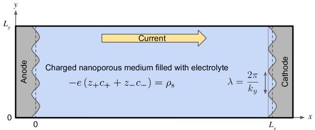
The starting point for modeling ion transport is the leaky membrane model that is able to predict overlimiting current carried by surface conduction, which we have previously coupled with Butler-Volmer reaction kinetics for analyzing steady state current-voltage relations and linear sweep voltammetry Khoo and Bazant (2018). The system under consideration is a binary asymmetric liquid electrolyte in a finite 3D charged random nanoporous medium where , and , whose 2D projection is illustrated in Figure 1. We assume that the nanoporous medium is random with well connected pores such as cellulose nitrate membranes so that we can investigate macroscopic electrode-scale morphological instabilities Han et al. (2016a). The cations are electroactive and the anions are inert. Initially, at , the anode surface is located at while the cathode surface is located at . As is typical for linear stability analysis of electrodeposition Sundström and Bark (1995); Elezgaray et al. (1998); Nielsen and Bruus (2015), we pick a moving reference frame with a velocity that is equal to the velocity of the electrode/electrolyte interface so that the average positions of the dissolving anode and growing cathode remain stationary. For the porous medium, we denote its porosity, tortuosity, internal pore surface area per unit volume and pore surface charge per unit area as , , and respectively. We assume that there are no homogeneous reactions and all material properties such as , , and are constant and uniform. We also assume that dilute solution theory holds true, hence all activity coefficients are and the cation and anion macroscopic diffusivities , where the subscript indicates dilute limit, are constant, uniform and independent of concentrations. Accounting for corrections due to the tortuosity of the porous medium, the macroscopic diffusivity is related to the molecular (free solution) diffusivity by Ferguson and Bazant (2012). The assumption of dilute solution theory further implies that the convective flux in the moving reference frame is negligible and the effect of the moving reference frame velocity is only significant in the equation describing electrode surface growth or dissolution Sundström and Bark (1995); Elezgaray et al. (1998); Nielsen and Bruus (2015), which we will discuss in Section II.3. Under these assumptions, for ion transport, the Nernst-Planck equations describing species conservation, charge conservation equation and macroscopic electroneutrality constraint are given by
| (1) | ||||
| (2) | ||||
| (3) |
where , , , are the cation and anion concentrations, fluxes and charge numbers respectively, is the electrolyte electric potential, is the electrolyte current density, is the effective pore size and is the volume-averaged background charge density. Denoting the numbers of cations and anions that are formed from complete dissociation of molecule of neutral salt as , electroneutrality requires that . We will use the macroscopic electroneutrality constraint given by Equation 3 to eliminate as a dependent variable, therefore leaving and as the remaining dependent variables.
For a classical system with an uncharged nanoporous medium, i.e., , the maximum current density that the system can possibly attain under electrodiffusion is called the diffusion-limited or limiting current density , which is given by Khoo and Bazant (2018)
| (4) |
where is the neutral salt bulk concentration. The limiting current is then given by where is the surface area of the electrode. Under galvanostatic conditions, when a current density larger than is applied, the cation and anion concentrations at the cathode reach and the electrolyte electric potential and electric field there diverge in finite time, which is called Sand’s time Sand (1899) denoted as ; see van Soestbergen et al. (2010) for a discussion of some subtlety associated with this transition time when is exactly equal to . If we have not assumed macroscopic electroneutrality and instead modeled electric double layers that can go out of equilibrium at high currents and voltages, then the electric field would be large but finite at and past Zaltzman and Rubinstein (2007); Nielsen and Bruus (2015); Bazant et al. (2005); Chu and Bazant (2005). Defining the dimensionless Sand’s time and dimensionless applied current density where Newman and Thomas-Alyea (2004); Khoo and Bazant (2018) is the ambipolar diffusivity of the neutral salt in the dilute limit and is the diffusion time scale, is given by van Soestbergen et al. (2010)
| (5) |
For galvanostatic conditions, is a critically important time scale because the formation of dendrites often occurs near or at , therefore it will be central to the linear stability analysis results discussed in Section IV.
Unlike the classical case of , for , the system can sustain an overlimiting current via surface conduction that is the electromigration of the counterions in the electric double layers (EDLs), which are formed next to the charged pore surfaces, under a large electric field generated in the depletion region next to the cathode. This additional surface conductivity thus enables the system to go beyond and eventually reach a steady state, in stark contrast to the finite time divergence of the classical case at . On the other hand, for , the counterions in the EDLs are the inert anions instead of the electroactive cations, which contribute a surface current that flows in the opposite direction from that of the bulk current. Because of this “negative” surface conductivity conferred by relative to , at the cathode, the bulk electrolyte concentration vanishes and the electric field diverges earlier than ; in other words, effectively reduces . A more quantitative way of explaining this is that the “negative” surface conductivity causes the maximum current density that can be achieved, which is denoted as , to be smaller than , and decreases as increases. In effect, a more positive decreases , which thus leads to a smaller for a given according to Equation 5. Details of how to numerically compute are found in Khoo and Bazant (2018); note that here corresponds to in Khoo and Bazant (2018).
II.2 Electrochemical reaction kinetics
In order to analyze how spatial perturbations of an electrode surface affect its linear stability, we need to account for the effects of surface curvature and surface energy in the electrochemical reaction kinetics model. The mean curvature of the electrode/electrolyte interface is given by where is the surface gradient operator and is the unit normal that points outwards from the electrolyte Deen (2011). In this paper, we consider a charge transfer reaction that involves only the cations and electrons while the anions are inert. More concretely, we suppose the following charge transfer reaction consuming electrons where is the oxidized species O with charge , is the electron e with charge , is the reduced species R with charge , and because of charge conservation. If the reduced species is solid metal, i.e., , as is the case in metal electrodeposition, the creation of additional electrode/electrolyte interfacial area results in a surface energy penalty that appears in the electrochemical potential of the reduced species. Therefore, the electrochemical potentials of the oxidized species O, electron e and reduced species R for are given by
| (6) | ||||
| (7) | ||||
| (8) |
where the surface energy term Sundström and Bark (1995); Elezgaray et al. (1998); Monroe and Newman (2003, 2004, 2005); Deen (2011); Tikekar et al. (2014); Nielsen and Bruus (2015) is included in when the reduced species is solid metal () and the superscript indicates standard state. The activity of species is given by where is the activity coefficient of species and is the concentration of species normalized by its standard concentration . is the standard electrochemical potential of species , is the electrode electric potential, is the atomic volume of the solid metal where and are the atomic mass and mass density of the metal respectively, and is the isotropic surface energy of the metal/electrolyte interface. The quantity is the capillary constant that has units of length Mullins and Sekerka (1963, 1964); Sekerka (1965). The interfacial electric potential difference is defined as . At equilibrium when , we obtain the Nernst equation
| (9) |
where the “eq” superscript denotes equilibrium and is the standard electrode potential. When the system is driven out of equilibrium so that , the system generates a Faradaic current density that is given by Bazant (2013, 2017); Ferguson and Bazant (2012)
| (10) |
where is the overall reaction rate constant and is the excess electrochemical potential of the transition state for the Faradaic reaction. Using the Butler-Volmer hypothesis, consists of a chemical contribution , where is the activity coefficient of the transition state for the Faradaic reaction, and a convex combination of the electrostatic energies, surface energies (only for the reduced species) and standard electrochemical potentials weighted by , which is the charge transfer coefficient. Therefore, is given by
| (11) |
Defining the overpotential as , we rewrite as
| (12) |
where is the exchange current density. In this form, we can identify the cathodic and anodic charge transfer coefficients, which are denoted as and respectively, as and such that . We note that our particular choice of in Equation 11 corresponds to choosing the “mechanical transfer coefficient” defined in Monroe and Newman (2004) to be equal to , causing to not depend explicitly on .
In this paper, we assume that the only charge transfer reaction occurring is metal electrodeposition that happens via the electrochemical reduction of cations in the electrolyte to solid metal on the electrode. The activity of solid metal is while we assume that the activity of electrons is . In addition, like in Section II.1, we assume that dilute solution theory is applicable, therefore the activity coefficients of the cation, anion and transition state for the Faradaic reaction are and we replace activities of the cation and anion with their normalized concentrations . Therefore, and simplify to
| (13) |
To compare the reaction and diffusion rates, we define the Damköhler number Da as the ratio of the Faradaic current density scale and limiting current density given by
| (14) |
When Da is large, i.e., , the system is diffusion-limited but when Da is small, i.e., , the system is reaction-limited.
II.3 Boundary conditions, constraints and initial conditions
We use “a” and “c” superscripts to denote the anode and cathode respectively, to denote the position vector, and to denote the positions of the anode and cathode. We ground the anode at all times, i.e., . Because the cations are electroactive, we impose no-flux boundary conditions for the cation flux on all boundaries except the anode and cathode where Faradaic reactions involving the cations occur. On the other hand, because the anions are inert, we impose no-flux boundary conditions for the anion flux on all boundaries. At the anode and cathode, we require the conservation of charges across the electrode/electrolyte interfaces. In summary, the boundary conditions are given by , , and where refers to all boundaries except the anode and cathode.
The velocity of the electrode/electrolyte interface is defined as and its normal component is given by . Because the growth (dissolution) of the electrode surface is caused by metal electrodeposition (electrodissolution), taking into account the moving reference frame velocity , the normal interfacial velocity is related to the normal current density by and therefore, .
For galvanostatic conditions in which we apply a current on the system, we require to satisfy charge conservation whereas for potentiostatic conditions in which we apply an electric potential on the cathode, we set . For initial conditions, we set where is the initial neutral salt bulk concentration Khoo and Bazant (2018), and and , i.e., the anode and cathode are initially planar.
III Linear stability analysis
III.1 Perturbations and linearization
Linear stability analysis generally involves imposing a spatial perturbation around a base state, keeping constant and linear terms of the perturbed state, and determining the dispersion relation that relates the growth rate of the perturbation to its wavenumber or wavelength. For electrodeposition specifically, the objective is to impose a spatial perturbation on a planar electrode surface and determine the effects of key system parameters on the linear stability of the surface in response to this perturbation. In this paper, we will choose a time-dependent base state, therefore the dispersion relation is also time-dependent. In 3D, the electrode/electrolyte interface can be written explicitly as where is the electrode surface height. Given , we can derive explicit expressions for surface variables such as the curvature and normal interfacial velocity in terms of and its spatial and temporal derivatives Deen (2011); Crank (1987), which are provided in Section I of Supplementary Material. For brevity, we let and where is the wavevector, and and are the wavenumbers in the and directions respectively. Therefore, , where is the -norm and is the overall wavenumber, and the wavelength is given by . For brevity again, we write the overall wavenumber as and it is obvious from context whether refers to the wavevector or overall wavenumber. The perturbation that will be imposed is sinusoidal in the and directions given by
| (15) |
where is a dimensionless small parameter, the and superscripts denote the base and perturbed states respectively, gives the real part of a complex number, is the complex-valued perturbation amplitude of the electrode surface height, and is the complex-valued growth rate of the perturbation. In response to such an electrode surface perturbation, we assume that the perturbations to and are similarly given by
| (16) | ||||
| (17) |
where and are the complex-valued perturbation amplitudes of anion concentration and electrolyte electric potential respectively.
To evaluate and and their gradients and at the interface at , we require their Taylor series expansions around the base state interface at . Letting and , these expansions are given by Sundström and Bark (1995); Elezgaray et al. (1998); Nielsen and Bruus (2015)
| (18) | ||||
| (19) | ||||
| (20) | ||||
| (21) |
After substituting these perturbation expressions into the full model in Section II, we obtain the base and perturbed states by matching the and terms respectively. The dispersion relation is subsequently computed by solving these and equations. The growth rate is generally complex-valued and for a particular value, there is an infinite discrete spectrum of values. However, for linear stability analysis, we are primarily interested in the maximum of the real parts of the values, which is denoted as , that corresponds to the most unstable eigenmode. If , the perturbation decays exponentially in time and the base state is linearly stable. On the other hand, if , the perturbation grows exponentially in time and the base state is linearly unstable. Lastly, if , the perturbation does not decay nor grow and the base state is marginally stable. The imposition of the boundary conditions at described in Section II.3 results in the quantization of the set of valid wavenumbers, which is explained in detail in Section IIIC of Supplementary Material.
III.2 Nondimensionalization
To make the equations more compact and derive key dimensionless parameters, in Table 1, we define the scales that are used for nondimensionalizing the full model in Section II and the perturbation expressions in Section III.1. and are the aspect ratios in the and directions respectively. For convenience, we also define (weighted ratio of cation and anion diffusivities), (ratio of atomic volume of solid metal to reciprocal electrolyte concentration), and (ratio of electrolyte concentration to standard cation concentration), and note that . Two important dimensionless parameters emerge from this nondimensionalization process, namely the Damköhler number that is described earlier in Equation 14 and the capillary number Ca that is given by
| (22) |
which is the ratio of the capillary constant Mullins and Sekerka (1963, 1964); Sekerka (1965) to the inter-electrode distance , and is the dimensionless isotropic surface energy of the metal/electrolyte interface.
| Variables and parameters | Scale |
| , , , , , , , , , | |
| (diffusion time) | |
| , , , , , | (thermal voltage) |
| , , , | |
| , | |
| , , , | |
| (reciprocal diffusion time) |
To avoid cluttering the notation, we drop tildes for all dimensionless variables and parameters, and all variables and parameters are dimensionless in the following sections unless otherwise stated. We also rewrite the and superscripts, which denote the base and perturbed states respectively, as and subscripts respectively. Similarly, we drop the subscript for diffusivities and the subscript for anion-related variables and parameters. As shorthand, we use subscripts to denote partial derivatives with respect to (with the exception that denotes the component of the moving reference frame velocity ), , and , primes to denote total derivatives with respect to , and an overhead dot to denote the total derivative with respect to . All equations for the dimensionless full model are provided in Section II of Supplementary Material. Details for deriving the dimensionless equations for the base and perturbed states are provided in Section III of Supplementary Material, and we summarize them in Sections III.3 and III.4 below.
III.3 Base state
The equations for the base state are obtained by substituting the perturbation expressions in Section III.1 into the full model in Section II and matching terms at . Equivalently, the base state is simply the full model specialized to 1D in the direction with the curvature-related terms dropped, which only appear at . Therefore, at , the governing PDEs (partial differential equations) are given by
| (23) | ||||
| (24) |
where the first PDE is the Nernst-Planck equation describing species conservation of anions and the second PDE is the charge conservation equation. The boundary conditions at the anode at are given by
| (25) | ||||
| (26) | ||||
| (27) | ||||
| (28) |
where , and . Since the unit normal at the cathode points in the opposite direction from that at the anode, the signs of the expressions involving at the cathode are opposite to that at the anode. Therefore, the boundary conditions at the cathode at are given by
| (29) | ||||
| (30) | ||||
| (31) |
where , and .
We pick and such that the positions of the anode and cathode in the base state remain stationary, i.e., . Therefore, where the second equality automatically holds true because of charge conservation in the 1D base state. Physically, is equal to the velocity of the growing planar cathode/electrolyte interface or the dissolving planar anode/electrolyte interface in the base state. The initial conditions are given by
| (32) |
Since , and at all . For galvanostatic conditions in which we apply a current density on the system, we impose
| (33) | ||||
| (34) |
For potentiostatic conditions in which we apply an electric potential on the cathode, we impose .
The equations for the time-dependent base state cannot generally be solved analytically, therefore we would have to solve them numerically. However, at steady state, the base state admits semi-analytical solutions for any Khoo and Bazant (2018). Specifically, , and their spatial derivatives can be analytically expressed in terms of the Lambert W function Corless et al. (1996). On the other hand, is known semi-analytically because it can be analytically expressed in terms of the Lambert W function up to an additive constant, which is a function of and and is found by numerically solving the algebraic Butler-Volmer equations given by Equations 27 and 30 with MATLAB’s or function.
III.4 Perturbed state
To derive the equations for the perturbed state at , we substitute the perturbation expressions in Section III.1 into the full model in Section II and match terms at . One important outcome is that the curvature-related terms appear as functions of because they are associated with second-order spatial partial derivatives in the and directions. At , the governing ODEs (ordinary differential equations) are given by
| (35) | |||
| (36) |
where the first ODE describes the perturbation in species conservation of anions and the second ODE describes the perturbation in charge conservation. For brevity, we define . The boundary conditions at the anode at are given by
| (37) | |||
| (38) | |||
| (39) |
where the , and parameters are
| (40) |
Because the unit normal at the cathode is in the opposite direction from that at the anode, the signs of the expressions involving at the cathode are opposite to that at the anode. Hence, the boundary conditions at the cathode at are given by
| (41) | |||
| (42) | |||
| (43) |
where the , and parameters are
| (44) |
The capillary number appears in the and parameters in the form of , which is the source of the surface stabilizing effect that arises from the surface energy penalty incurred in creating additional surface area. The competition between this surface stabilizing effect and the surface destabilizing effect arising from the , and fields sets the scale for the critical wavenumber , which is the wavenumber at which the perturbation growth rate is and the electrode surface is marginally stable.
III.5 Discretization of perturbed state
Without making further approximations, the equations for the perturbed state do not admit analytical solutions, thus we have to resort to numerical methods to solve them. To do so, the equations for the perturbed state are spatially discretized over a uniform grid with grid points and a grid spacing using second-order accurate finite differences LeVeque (2007). Details of this discretization process are provided in Section IV of Supplementary Material. In summary, the discretized equations can be written as a generalized eigenvalue problem given by
| (45) |
where , , and the second subscript in and for denotes the grid point index. In the context of a generalized eigenvalue problem, the eigenvector consists of the complex-valued amplitudes , , and evaluated at the grid points, and the eigenvalue is the complex-valued growth rate . Although is non-singular, the time-independent terms in the equations for the perturbed state introduce rows of zeros in , therefore is singular and the generalized eigenvalue problem cannot be reduced to a standard eigenvalue problem. Specifically, is non-singular with rank while is singular with rank , and the total number of eigenvalues is .
Because is singular with rank , there are finite eigenvalues and infinite eigenvalues. This mathematical property is not always consistently noted in past literature on linear stability analysis of electrodeposition, although Sundström and Bark did mention that different eigenvalues are obtained with grid points that give rise to equations without explicitly stating that the other eigenvalues are infinite Sundström and Bark (1995). The infinite eigenvalues are physically irrelevant to the linear stability analysis Valério et al. (2007); Kawano et al. (2013), therefore we would want to focus on solving for the finite eigenvalues. This can be achieved by mapping the infinite eigenvalues to other arbitrarily chosen points in the complex plane via simple matrix transformations Goussis and Pearlstein (1989). Details of how these transformations are performed are given in Section IV of Supplementary Material. There are methods for directly removing the infinite eigenvalues such as the “reduced” method Gary and Helgason (1970); Peters and Wilkinson (1970); Valério et al. (2007) but they are more intrusive and require more extensive matrix manipulations as compared to the mapping technique Goussis and Pearlstein (1989) that we use.
The modified generalized eigenvalue problem that results from these transformations can then be solved using any eigenvalue solver. For linear stability analysis, we only need to find the eigenvalue with the largest real part instead of all the finite eigenvalues. Since the time complexity of finding all the eigenvalues typically scales as while that for finding of them, where in our case, scales as , the computational cost is dramatically reduced by a factor of if we use an eigenvalue solver that can find subsets of eigenvalues and eigenvectors such as MATLAB’s solver.
III.6 Numerical implementation
The equations for the time-dependent base state in Section III.3 are numerically solved using the finite element method in COMSOL Multiphysics 5.3a. The eigenvalue with the largest real part and its corresponding eigenvector from the generalized eigenvalue problem for the perturbed state in Section III.5 are then solved for using the function in MATLAB R2018a. When the function occasionally fails to converge for small values of the wavenumber , we use Rostami and Xue’s eigenvalue solver based on the matrix exponential Rostami and Xue (2018); Xue , which is more robust than the function. The colormaps used for some of the plots in Section IV are obtained from BrewerMap Cobeldick , which is a MATLAB program available in the MATLAB File Exchange that implements the ColorBrewer colormaps Harrower and Brewer (2003).
IV Results
Because of the large number of dimensionless parameters present, the parameter space is too immense to be explored thoroughly in this paper. Instead, the key dimensionless parameters that we focus on and vary are , Da and under galvanostatic conditions. corresponds to the classical case of an uncharged nanoporous medium while allows us to depart from this classical case and study its effects on the linear stability of the electrode surface. Experimentally, can be tuned via layer-by-layer deposition of polyelectrolytes Han et al. (2014, 2016a); Hammond (2004) or tethered immobilized anions Tu et al. (2015). Da is very sensitive to the specific reactions considered and varies significantly in practice. We focus on galvanostatic conditions instead of potentiostatic conditions because when an overlimiting current is applied on a classical system with , as discussed in Section II.1, the Sand’s time provides a time scale at which the electric field at the cathode diverges that causes the perturbation growth rate to diverge too. This allows us to focus the linear stability analysis on times immediately before, at and immediately after .
For the results discussed in Sections IV.2, IV.3, IV.4 and IV.6 below, we assume the following dimensional quantities for a typical electrolyte in a typical nanoporous medium: , (arbitrarily pick lithium metal) Rumble (2017), (arbitrarily pick lithium metal) Rumble (2017), , ( to model a thin gap cell that reduces effects of gravity-induced convection (buoyancy) Elezgaray et al. (1998)), (note that here is the dimensional initial neutral salt bulk concentration, not the dimensionless base state anion concentration), (standard concentration) and (typical surface energy of metal/electrolyte interface) Sundström and Bark (1995). Corresponding to these dimensional quantities, all dimensionless parameters that are used for the results in Sections IV.2, IV.3, IV.4 and IV.6 are given in Table 2.
| Dimensionless parameter | Description | Value |
| Number of cations formed from complete dissolution of 1 molecule of neutral salt | ||
| Number of anions formed from complete dissolution of 1 molecule of neutral salt | ||
| Cation charge number | ||
| Anion charge number | ||
| Cation diffusivity | ||
| Anion diffusivity | ||
| Number of electrons transferred in charge transfer reaction | ||
| Charge transfer coefficient | ||
| Capillary number, ratio of capillary constant to inter-electrode distance (Equation 22) | ||
| Ratio of atomic volume of solid metal to reciprocal electrolyte concentration | ||
| Weighted ratio of cation and anion diffusivities | ||
| Ratio of to | ||
| Ratio of electrolyte concentration to standard cation concentration | ||
| Standard electrode potential | ||
| Aspect ratio in direction | ||
| Aspect ratio in direction | ||
| Ratio of background charge density to electrolyte concentration | , | |
| Da | Damköhler number, ratio of reaction rate to diffusion rate (Equation 14) |
IV.1 Approximations
At the heart of the linear stability analysis is the competition between the destabilizing effect that arises from the amplification of surface protrusions by diffusive fluxes in a positive feedback loop and the stabilizing effect that arises from the surface energy penalty incurred in the creation of additional surface area. Therefore, in the dispersion relation , we expect to see some local maxima or possibly just a single global maximum, which we denote as , where the electrode surface is maximally unstable. We also expect to see a critical wavenumber corresponding to where the electrode surface is marginally stable. When is larger than , is always negative because the surface energy stabilizing effect always dominates when the wavenumber is sufficiently large. We note that is always greater than . Corresponding to and are the maximum wavelength and critical wavelength respectively. In a porous medium, the characteristic pore size , where is the pore diameter, sets a threshold or cutoff for overall electrode surface stabilization: we should observe stabilization if is smaller than Tikekar et al. (2014). If is larger than , then the most unstable eigenmode dominates the electrode surface growth with a growth rate of and the characteristic length scale of this instability is . Therefore, and are the most physically informative points of the dispersion relation. We now derive an approximation for the dispersion relation that is valid at high values of relative to and will be useful for computing and quickly and accurately because and tend to be large. The approximation is also useful for verifying the full numerical solution at high , which will be discussed in Section IV.2.
When is sufficiently large compared to , at the cathode at , we expect to balance , and to balance in Equations 35 and 36 respectively. Therefore, is a small parameter multiplying the highest order spatial derivative terms and , and the spatial profiles for and form a boundary layer with characteristic thickness . Hence, as an ansatz for the boundary layer analysis, we assume
| (46) |
where and are arbitrary constants that are determined from the boundary conditions at . By assuming such an ansatz, the cathode is effectively decoupled from the anode and the perturbation growth rate is entirely dependent on the boundary conditions at the cathode. The validity of this ansatz is corroborated by our observations that generally in our numerical simulations, especially at large values of , which was also observed by Sundström and Bark Sundström and Bark (1995). Imposing the boundary conditions at , we obtain
| (47) | ||||
| (48) | ||||
| (49) |
where we define , and for brevity.
Approximate values of can be obtained by solving and requiring where the primes indicate total derivatives with respect to . In addition, by solving , we can obtain approximate values of . However, this process is tedious because the first term inside the braces in Equation 49 is a rational function that consists of polynomials in of relatively high degrees. Specifically, after multiplying the numerator and denominator of this term by , it becomes a rational function with a numerator that is a polynomial in of degree and a denominator that is a polynomial in of degree . Therefore, for the purpose of quickly approximating and , we first find a simpler and yet still accurate analytical approximation for , which can then used as an initial guess for numerically solving for using Equation 49 with MATLAB’s optimizer. Such an approximation can be obtained by assuming is large enough that and and then setting in Equation 42, thus resulting in
| (50) |
We observe that scales as , which is expected because the surface energy stabilizing effect appears in the form of in in Equation 42, and this scaling agrees with that obtained in previous work done on linear stability analysis of electrodeposition Sundström and Bark (1995); Elezgaray et al. (1998); Krishnan et al. (2002); Tikekar et al. (2014); Nielsen and Bruus (2015).
IV.2 Convergence analysis
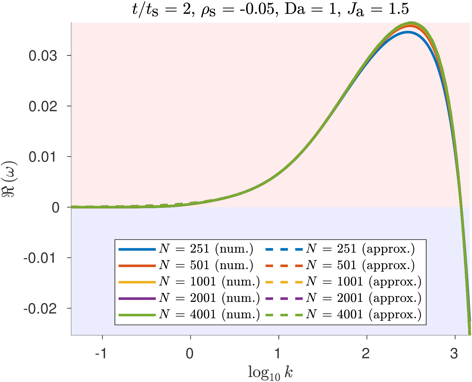
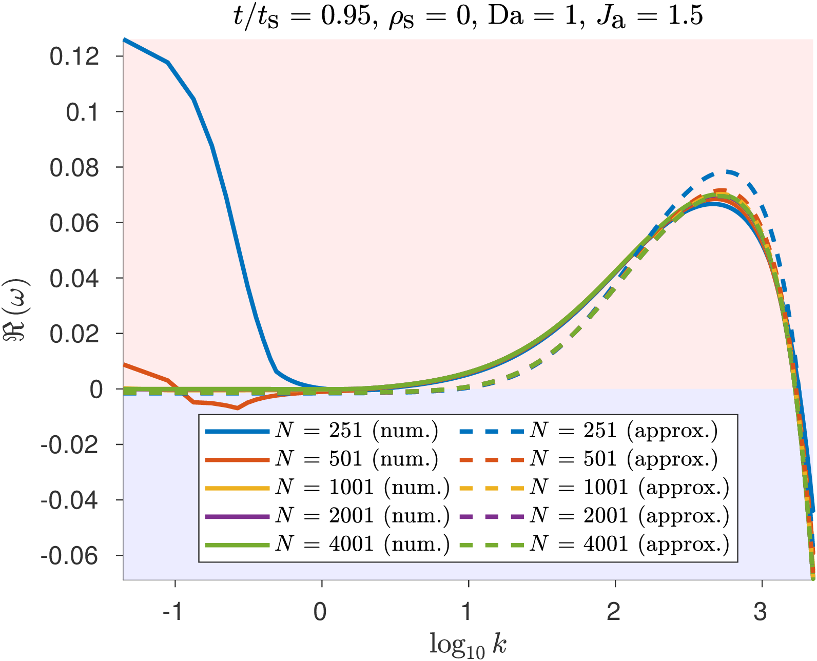
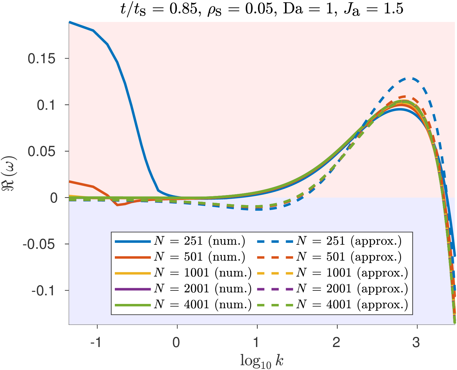
Before analyzing the physical significance of the linear stability analysis results, we would want to first establish the accuracy and convergence of the full numerical solution of the dispersion relation . To this end, we perform a numerical convergence analysis in which we examine the convergence of the numerical solution as the number of grid points increases. At the same time, we also compute the approximate given by Equation 49 because we expect the numerical and approximate solutions to agree well at high values of ; this therefore provides another way of checking the accuracies of both the numerical and approximate solutions.
To demonstrate how the numerical dispersion relation changes with , we fix and (overlimiting current) and plot numerically computed against for and at specific values in Figure 2. As expected, the numerical solutions converge quickly as increases from to . For and at small values of , when the value of is small at or , we observe that there are anomalously large values of that vanish at larger values of . This is because when is too small, the grid is not sufficiently fine to accurately resolve the base state variables, in particular the rapidly increasing electric field at the cathode near , thus leading to an overestimation of the destabilizing effect caused by electrodiffusion and an underestimation of the stabilizing effect caused by surface energy. The numerical and approximate solutions also expectedly agree well with each other at large values of and this agreement improves as increases, thus confirming that the approximations are accurate at high .
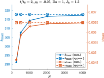
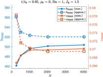
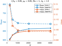
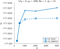
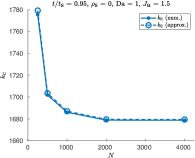
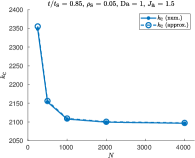
Because we are mostly interested in the , and points on the curve, we plot them against in Figure 3. We observe that the numerically computed , and curves rapidly level off and converge to constant values as increases. The numerical and approximate solutions also agree very well as increases, which is expected because and are large and the approximations are accurate at high . As a compromise between numerical accuracy and computational time, we pick for all numerical and approximate solutions computed in the following sections.
IV.3 Parameter sweeps
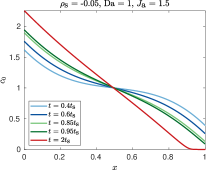
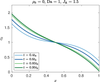
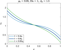
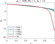
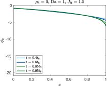
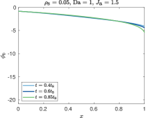
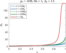
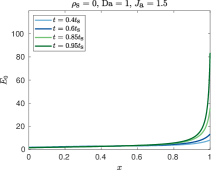
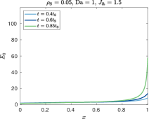
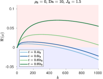
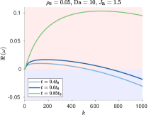
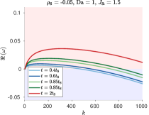
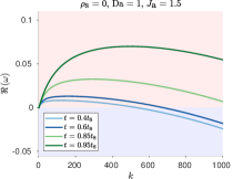
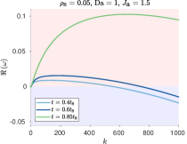
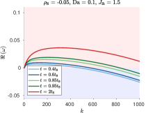
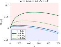
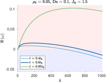
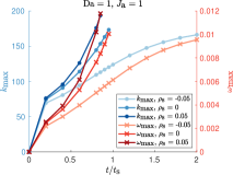
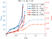
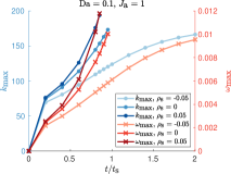
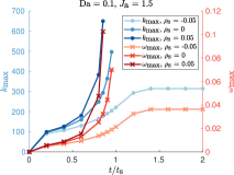
The base state anion concentration field , electrolyte electric potential field and electric field possess salient features that are useful for understanding the linear stability analysis results. We focus on galvanostatic conditions under an overlimiting current because as explained in Section II.1, doing so provides us with Sand’s time as a time scale at which the bulk electrolyte is depleted at the cathode. Depending on the sign of , the , and fields behave differently at and beyond. Fixing and (overlimiting current), we plot , and against for various values for in Figure 4. For , because the system can go beyond and eventually reach a steady state, we show plots up to . For , since and at the cathode diverge at , which cause the numerical solver to stop converging, we can only show plots up to . For , because effectively reduces as discussed in Section II.1, we show plots up to .
For , the distinguishing features of running the system at an overlimiting current carried by surface conduction are the anion depletion region at the cathode and the bounded and constant electric field in this depletion region after . Because the anion concentration gradient almost vanishes in the depletion region, the current in this region is predominantly not carried by electrodiffusion but by electromigration of the counterions in the electric double layers (EDLs) under the aforementioned bounded and constant electric field , i.e., surface conduction. Moreover, because of this additional surface conductivity, when compared to and , is always smaller at all for a given . On the other hand, for the classical case of , at the cathode quickly increases near and eventually diverges at . Relative to this classical case, for , is always greater at all for a given and eventually diverges at the cathode earlier than because of the “negative” surface conductivity conferred by the positive background charge as discussed in Section II.1.
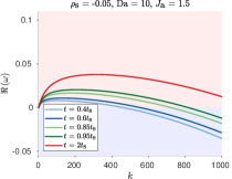
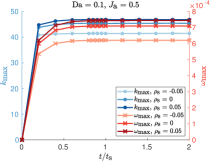
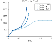
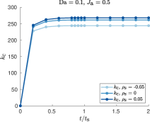
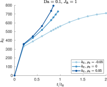
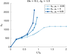
We now examine the dispersion relation by plotting numerically computed against for various values for , and (overlimiting current) in Figure 5. In Figure 5, increases from left to right and Da increases from bottom to top. Generally for all the parameters considered, the curve, in particular the , and points, increases and “moves in the northeast direction” as increases; qualitatively, the “total amount of instability” increases with . For , when compared to and , the curve is the smallest at a given because of a smaller base state electric field . The curve also remains bounded at all and eventually reaches a steady state that is almost attained near because at the cathode behaves in the same fashion. In sharp contrast, for the classical case of near , the curve grows dramatically because of the rapidly increasing at the cathode, which eventually diverges at and in turn causes the curve to diverge at too. Compared to this classical case, for , because at the cathode is larger at a given and diverges earlier than , the curve accordingly grows even more rapidly at earlier times and diverges earlier than . Therefore, by bounding the electric field at the cathode, the presence of a negative background charge confers additional stabilization to the system beyond what is provided by surface energy effects, although it does not completely stabilize the system as there are still regions of positive growth rate in the dispersion relation. On the other hand, for the classical case of zero background charge, the system rapidly destabilizes near Sand’s time and ultimately diverges at Sand’s time because of the diverging electric field at the cathode, which is also demonstrated in Elezgaray et al. (1998). Relative to this classical case, the presence of a positive background charge destabilizes the system even further by generating an electric field at the cathode that is larger at a given time and diverges earlier than Sand’s time, resulting in higher growth rates at earlier times and in finite time divergence earlier than Sand’s time.
We observe that increasing Da generally increases but this effect is very insignificant because the application of an overlimiting current implies that the system is always diffusion-limited regardless of what Da is. Hence, in this regime of diffusion-limited electrodeposition under an overlimiting current, specific details of the electrochemical reaction kinetics model are not important in influencing the dispersion relation as long as the model includes the surface energy stabilizing effect, which typically occurs in the functional form of .
In the interest of space, plots of numerically computed against for (limiting current) and (underlimiting current) are not shown here but are given in Figures 1 and 2 in Section V of Supplementary Material respectively. Since the system is still always diffusion-limited for , the trends observed for are qualitatively similar to our previous discussion for , except that the values are smaller because a smaller applied current density results in a smaller electric field at the cathode. For , because the applied current density is underlimiting, Sand’s time is not defined and at the cathode, the bulk electrolyte concentration does not vanish and the electric field does not diverge at any . Therefore, the curve remains bounded at all and reaches a steady state eventually. Moreover, generally increases with Da, and this increase is especially pronounced when Da increases from to ; this effect was also observed by Sundström and Bark Sundström and Bark (1995) who focused their analysis on underlimiting currents. This increase in is not directly caused by because does not change appreciably despite the increase in Da (refer to Figures 3 to 5 in Section VI of Supplementary Material). Rather, as discussed in Section II.2, the system becomes diffusion-limited when , causing the surface perturbations to destabilize faster.
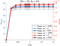
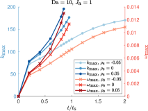
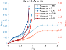
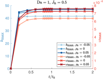
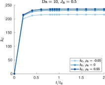
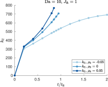
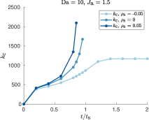
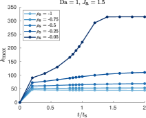
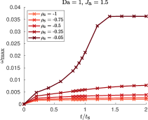
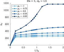
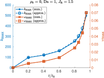
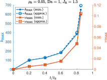
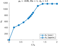
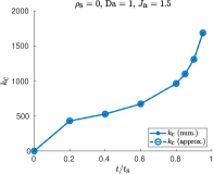
As discussed in Section IV.1, at each point, each curve exhibits a global maximum and a critical wavenumber , which is where the curve crosses the horizontal axis . The and points provide a succinct way to summarize the most physically significant features of the curve for all the parameter ranges we have explored thus far. Therefore, for , and , we plot numerically computed and against in Figure 6 and numerically computed against in Figure 7. For , we observe that the and curves diverge near for but level off to constant values past for , therefore these curves appear as if they are “fanning out”. In contrast, for , the and curves level off past for all values of as the system eventually reaches a steady state when an underlimiting current is applied. The curves have the same qualitative shape as the curves except that they are larger, as expected. The effects of Da and on the , and values, which are previously discussed in the context of the dispersion relation, are also clearly reflected in Figures 6 and 7.


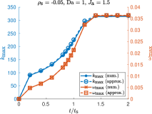
In an effort to make the electrode surface less unstable at overlimiting current, we focus on to determine how much additional stabilization a negative confers to the surface as it gets increasingly more negative. Subsequently, we plot numerically computed , and against for , and in Figure 8. While a more negative generally decreases , and , it is clear that there are diminishing returns to the amount of additional stabilization achieved. It also appears that complete stabilization is not possible as remains positive even for , albeit at a small value. In practice, it is probable that a sufficiently small and positive value can be deemed to be small enough for considering an electrode surface “practically stable”, but experiments that measure and correlate with observations of metal growth need to be performed in order to determine this threshold value.
IV.4 Comparison between numerical and approximate solutions
To illustrate how well the approximations given by Equations 49 and 50 work for the parameter ranges considered, we plot numerical and approximate values of , and against for , and in Figure 9. In the interest of space, these plots for other values of Da and are provided in Figures 6 to 11 of Section VII of Supplementary Material. For all parameter ranges considered, the agreement between numerical and approximate values of , and is excellent, giving us confidence that the approximations are useful for rapidly and accurately computing , and . This confirms that and are large enough that Equations 49 and 50, which have assumed that is sufficiently large, are accurate for approximating them. We will therefore use Equations 49 and 50 extensively in Sections IV.5 and IV.6 that follow.
IV.5 Application to copper electrodeposition
We now apply linear stability analysis to the specific case of copper electrodeposition and electrodissolution and compare it with experimental data Han et al. (2016a) to determine how well theory agrees with experiment. Because copper electrodeposition involves the overall transfer of two electrons that are transferred one at a time in a serial manner, we need to first derive the overall expression for the Faradaic current density .
Assuming that the activity of electrons is and dilute solution theory is applicable, for a -electron transfer reaction, the dimensionless forms of Equations 12 and 9 are given by
| (51) | ||||
| (52) |
For multistep electron transfer reactions, it is more convenient to work with instead of . Therefore, we rewrite in terms of as
| (53) | ||||
| (54) |
where and are the cathodic and anodic rate constants respectively.
The reaction mechanism for copper electrodeposition and electrodissolution is given by Newman and Thomas-Alyea (2004); Mattsson and Bockris (1959); Bockris and Enyo (1962); Brown and Thirsk (1965)
| (55) | ||||
| (56) |
where (aq), (ads) and (s) indicate aqueous, adsorbed and solid respectively. The first step is assumed to be the rate-determining step while the second step is assumed to be at equilibrium. Applying Equation 53 to each step, noting that the activity of solid metal is and rewriting in terms of , we obtain
| (57) | ||||
| (58) |
where is the charge transfer coefficient of the first step.
Previously in Section II.2, for a -step -electron transfer metal electrodeposition reaction, the dimensionless forms of Equations 12 and 13 are given by
| (59) | ||||
| (60) |
By comparing Equations 57 and 58 with Equations 59 and 60, we set and and replace with in the original set of equations in order to adapt the linear stability analysis for copper electrodeposition.
By carrying out nonlinear least squares fitting on experimental steady state current-voltage relations, we have previously performed parameter estimation Khoo and Bazant (2018) for copper electrodeposition in a copper(II) sulfate () electrolyte in cellulose nitrate (CN) membranes Han et al. (2016a), which are a random nanoporous medium with well connected pores. The parameters that are estimated are , , Da, and and their fitted values are provided in Table III in Khoo and Bazant (2018). Other parameters specific to the copper electrodeposition reaction, electrolyte and CN membranes used are also provided in Tables I and II in Khoo and Bazant (2018). For the surface energy of the copper/electrolyte interface, we use dimensional given in Table I in Nielsen and Bruus (2015).
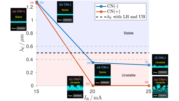
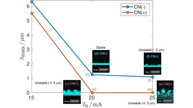
For our analysis here, the specific experimental datasets that we focus on are labeled and in Khoo and Bazant (2018), which correspond to negatively and positively charged CN membranes respectively with a dimensional electrolyte concentration of . We will drop the subscript for brevity. The morphologies of the electrodeposited copper films, which are visualized by EDS (energy dispersive X-ray spectroscopy) maps, for these and membranes at for dimensional applied currents of , and are given in Figure 10(a) that consists of magnifications of EDS maps taken from Figures 6(a) to 6(f) of Han et al. (2016a). At , the copper films for both and membranes appear to be uniform and stable. However, at and , the film for becomes very unstable and roughens more as the applied current increases. It is difficult to determine quantitatively the instability wavelength using the relatively low resolution EDS maps but it is probably much smaller than . In contrast, for , the film still remains uniform and stable at but slightly destabilizes and roughens at with an instability wavelength probably on the order of . In summary, the onset of overall electrode surface destabilization occurs at for with an instability wavelength of much smaller than and at for with an instability wavelength of about .
Because the EDS maps are taken at , which is much longer than the diffusion times for and of and respectively, we assume that the system is at steady state. This assumption allows us to use the semi-analytical expressions for the base state variables in Khoo and Bazant (2018), which we have previously discussed in Section III.3, to compute approximate values of and using Equations 49 and 50. The dataset has a dimensional limiting current of while the dataset has a dimensional maximum current, which we have discussed in Section II.1, of . Therefore, for , the three applied currents of , and correspond to underlimiting, slightly overlimiting and overlimiting currents respectively. On the other hand, for , the model eventually diverges and does not admit a steady state when the applied current is above the maximum current , therefore we can only obtain finite values of and for the applied current of while the model predicts infinite values of and for the applied currents of and due to finite time divergence of the system. Other fitted key dimensionless parameters include and for and and for .
To summarize the model predictions, we plot approximate dimensional values of and against the dimensional applied current in Figure 10. In the plot in Figure 10(a), we also indicate the characteristic pore size of , which is given by twice the pore diameter of Han et al. (2016a), in order to determine if the model predicts overall electrode surface stabilization. As discussed in Section IV.1, we expect overall electrode surface stabilization if , which corresponds to the blue shaded region in the plot. On the contrary, we expect overall electrode surface destabilization if , which corresponds to the red shaded region in the plot, and the characteristic instability wavelength is . Comparing the plot with our previous discussion of the onset of overall electrode surface destabilization suggested by the copper film morphologies observed experimentally, we see that the model generally agrees well with experiment; the only disagreement is at where the model predicts destabilization for , which has , while the EDS map of the copper film at this applied current shows that the film appears to be stable. Nonetheless, this disagreement in theory and experiment is relatively minor since for at is only slightly smaller than the mean of of and is almost equal to the lower bound of of . In addition, the model predicts (because when ) at and for while it predicts at for . These model predictions of qualitatively agree well with the experimentally observed instability wavelengths at these applied currents that we have previously discussed. Therefore, in conclusion, the theory agrees reasonably well with experimental data, especially given that many assumptions and simplifications are made in the model.
(a)
(b)
IV.6 Pulse electroplating and pulse charging
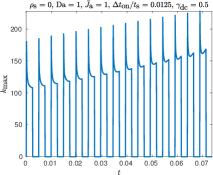
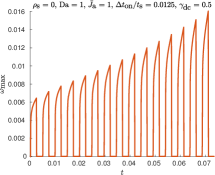
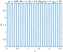
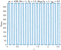
For many electrochemical applications such as electroplating and charging of metal batteries, which is equivalent to electrodeposition at the metal negative electrode, it is desirable to operate them as quickly as possible at a high current without causing the formation of dendrites that short-circuit the system. To delay or prevent the formation of dendrites, it is common to perform pulse electroplating of metals Devaraj et al. (1990); Chandrasekar and Pushpavanam (2008) or pulse charging of lithium metal batteries (LMBs) and lithium-ion batteries (LIBs) Li et al. (2001); Purushothaman et al. (2005); Purushothaman and Landau (2006); Zhang (2006); Hussein and Batarseh (2011); Shen et al. (2012); Savoye et al. (2012); Mayers et al. (2012); Aryanfar et al. (2014) so that there is sufficient time between pulses for the concentration gradients and electric field in the system to relax. For pulse electroplating of metals, it has been empirically observed that the crystal grain size generally decreases with applied current Devaraj et al. (1990); Chandrasekar and Pushpavanam (2008). Using an applied direct current to perform silver electrodeposition under galvanostatic conditions, Aogaki experimentally observed that the crystal grain size decreases with time Aogaki (1982a, b), which agrees well with theoretical predictions from linear stability analysis previously done by Aogaki and Makino Aogaki and Makino (1981). With all these considerations in mind, we apply our linear stability analysis with a time-dependent base state as a tool to investigate how pulse electroplating protocols with high average applied currents, which are inherently time-dependent, affect the linear stability of the electrode surface and the crystal grain size for both zero and negative pore surface charges.
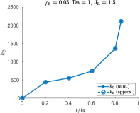
Based on the results in Section IV.5, we generally expect the characteristic pore size to be larger than the critical wavelength at high applied currents, therefore the electrode surface is unstable with a characteristic instability wavelength . Because a pulse current is applied, varies in time and hence, it would be useful to define an average that averages out the effect of time. In this spirit, we define the average maximum wavenumber and the corresponding average maximum wavelength as
| (61) |
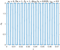
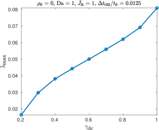
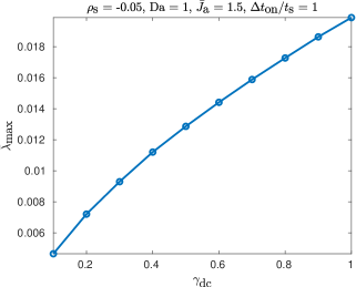
where is the final time of the pulse and each maximum wavenumber is weighted by its corresponding maximum growth rate . We expect to be on the same order of magnitude as the the crystal grain size that is observed experimentally. As a simple example, we suppose that the pulse electroplating protocol is a periodic pulse wave with an “on” (charging) time of , a “off” (relaxation) time of , and a period given by . The duty cycle is given by and the average applied current density over one period is given by where is the peak applied current density. Hence, for a particular , a smaller implies a larger .
For the classical case of , we pick and and vary from to (direct current) where the Sand’s time is calculated based on . , and should be carefully chosen such that is not too high to deplete the bulk electrolyte at the cathode during the “on” cycle so that the system does not diverge at any point in time; this explains why for our choice of and cannot be numerically simulated. For , we pick and and vary from to (direct current) to drive the system at an overlimiting average applied current density. We also fix for both cases and use Equations 49 and 50 to compute approximate values of and . For these choices of parameters, as an illustrative example, we plot , approximate and approximate against for in Figure 11. We note that the large overshoot in at the beginning of each “on” cycle for is caused by the sharp rate of increase of the concentration gradients and electric field as rapidly increases from in the “off” cycle to in the “on” cycle. Corresponding to these pulse waves, we plot against in Figure 12. For both and , increases with , which agrees with the empirical observation that the crystal grain size generally decreases with applied current Devaraj et al. (1990); Chandrasekar and Pushpavanam (2008). The ability to experimentally impart a negative pore surface charge to the nanoporous medium therefore enables pulse electroplating at overlimiting currents for electrodepositing a large amount of charge at a high rate and tuning the desired crystal grain size.

V Conclusion
We have derived the full model that couples the leaky membrane model for ion transport, which is capable of predicting overlimiting current due to surface conduction, with Butler-Volmer reaction kinetics, which describes the metal electrodeposition reaction, and performed linear stability analysis on it with respect to a time-dependent base state. The volume-averaged background charge density can generally be of any sign. As a result, we have generalized previous work on linear stability analysis of electrodeposition carried out in Sundström and Bark (1995); Elezgaray et al. (1998); Tikekar et al. (2014). We then performed a boundary layer analysis on the perturbed state in order to derive an accurate approximation for the dispersion relation and a convergence analysis to verify the accuracy and convergence of the full numerical solution of the dispersion relation. By performing parameter sweeps over the volume-averaged background charge density, Damköhler number and applied current density under galvanostatic conditions, we have concluded that a negative background charge significantly stabilizes the electrode surface instability, although it does not completely stabilize it, while a positive background charge further destabilizes this instability. We have also verified that the approximations for the maximum wavenumber, maximum growth rate and and critical wavenumber are very accurate, and applied them to demonstrate good agreement between theory and experimental data for copper electrodeposition in cellulose nitrate membranes Han et al. (2016a). Lastly, we have employed the linear stability analysis as a tool to analyze the dependence of the crystal grain size on duty cycle in pulse electroplating. These results demonstrate the predictive power and robustness of the theory despite its simplicity. Although detailed analysis of the Poisson-Nernst-Planck-Stokes equations for transport in a microchannel by Nielsen and Bruus Nielsen and Bruus (2014) reveals that the leaky membrane model for surface conduction is at best a rough approximation of the real system, the good agreement between theory and experiment that we have demonstrated suggests that the model is applicable in similar electrochemical systems using charged membranes such as shock electrodeposition for information storage applications Han et al. (2016b) and shock electrodialysis for water treatment Deng et al. (2013); Schlumpberger et al. (2015); Schlumpberger (2016).
We have made many assumptions and simplifications in the model presented, and relaxing some of them offers opportunities for extending it in useful ways. First, we have ignored surface adsorption, surface diffusion of adsorbed species Aogaki and Makino (1984a, b, c, d) and additional mechanical effects such as pressure, viscous stress and deformational stress Monroe and Newman (2004, 2005); Tikekar et al. (2016b); Ahmad and Viswanathan (2017a, b); Natsiavas et al. (2016), which confer additional stabilization to the electrode surface. Adding these physics and chemistry to the model are likely to result in finite values of the maximum wavenumber, maximum growth rate and critical wavenumber near and at Sand’s time under an overlimiting current for zero and positive background charges respectively, as opposed to diverging in our current model. The inclusion of these additional mechanical effects will also extend the applicability of the model to solid electrolytes Liu et al. (2017) that are used in solid state batteries. Deformation of the porous medium caused by metal growth inside the pores also results in a porosity that varies in both time and space whose effects would be interesting to study. Second, in order to apply the linear stability analysis to lithium metal batteries (LMBs), we would also need to model the solid electrolyte interphase (SEI) layer Verma et al. (2010); Cheng et al. (2016); Peled and Menkin (2017); Wang et al. (2018), which will certainly increase the complexity of the model but also make it more predictive. Incorporating these two aforementioned extensions into the model may help explain recent experimental studies of lithium growth that have demonstrated that competing SEI reactions and stress effects lead to root growth before Sand’s time or below limiting current Bai et al. (2016); Kushima et al. (2017); Bai et al. (2018), which is different from tip growth of dendrites under transport limitation that we have focused on in this paper. Third, other chemical mechanisms for overlimiting current such as water splitting Nikonenko et al. (2010, 2014) and current-induced membrane discharge Andersen et al. (2012) may be present. These effects are typically highly nonlinear and therefore, we expect them to significantly influence the transient base state and linear stability analysis. Fourth, we should consider the effects of coupling nucleation, which is fundamentally a nonlinear instability unlike spinodal decomposition that is a linear instability, to the current model. Specifically, nucleation may affect the transient base state during initial and early reaction-limited surface growth and create surface roughness on the scale of the characteristic nucleus size, which may in turn influence overall electrode surface stabilization or destabilization when the system reaches transport limitation near or at Sand’s time. Fifth, an interesting and useful generalization of the reaction model would be to use the symmetric Marcus-Hush-Chidsey kinetics Bai and Bazant (2014); Zeng et al. (2014) or asymmetric Marcus-Hush kinetics Zeng et al. (2015) instead of Butler-Volmer kinetics for modeling electron transfer reactions, which would afford us the reorganization energy as a key system parameter whose influence on the linear stability of the electrode surface can be investigated.
Acknowledgements.
E. Khoo acknowledges support from the National Science Scholarship (PhD) funded by Agency for Science, Technology and Research, Singapore (A*STAR). H. Zhao and M. Z. Bazant acknowledge support from the Toyota Research Institute through the D3BATT Center on Data-Driven-Design of Rechargeable Batteries.References
- Langer (1980) J. S. Langer, Reviews of Modern Physics 52, 1 (1980).
- Kessler et al. (1988) D. A. Kessler, J. Koplik, and H. Levine, Advances in Physics 37, 255 (1988).
- Cross and Hohenberg (1993) M. C. Cross and P. C. Hohenberg, Reviews of Modern Physics 65, 851 (1993).
- Orr (1907a) W. M. Orr, Proceedings of the Royal Irish Academy. Section A: Mathematical and Physical Sciences 27, 9 (1907a).
- Orr (1907b) W. M. Orr, Proceedings of the Royal Irish Academy. Section A: Mathematical and Physical Sciences 27, 69 (1907b).
- Sommerfeld (1908) A. Sommerfeld, Atti del 4, 116 (1908).
- Orszag (1971) S. A. Orszag, Journal of Fluid Mechanics 50, 689 (1971).
- Zaltzman and Rubinstein (2007) B. Zaltzman and I. Rubinstein, Journal of Fluid Mechanics 579, 173 (2007).
- Ben-Jacob and Garik (1990) E. Ben-Jacob and P. Garik, Nature 343, 523 (1990).
- Lopez-Tomas et al. (1995) L. Lopez-Tomas, J. Mach, P. P. Trigueros, F. Mas, J. Claret, and F. Sagues, Chaos, Solitons & Fractals Complex Systems in Computational Physics, 6, 287 (1995).
- Léger et al. (1999a) C. Léger, L. Servant, J. L. Bruneel, and F. Argoul, Physica A: Statistical Mechanics and its Applications Proceedings of the 20th IUPAP International Conference on Statistical Physics, 263, 305 (1999a).
- Sagués et al. (2000) F. Sagués, M. Q. López-Salvans, and J. Claret, Physics Reports 337, 97 (2000).
- Rosso et al. (2003) M. Rosso, E. Chassaing, V. Fleury, and J.-N. Chazalviel, Journal of Electroanalytical Chemistry International Symposium on Materials Processing for Nanostructured Devices 2001, 559, 165 (2003).
- Schwarzacher (2004) W. Schwarzacher, Journal of Physics: Condensed Matter 16, R859 (2004).
- Rosso (2007) M. Rosso, Electrochimica Acta ELECTROCHEMICAL PROCESSING OF TAILORED MATERIALS Selection of papers from the 4th International Symposium (EPTM 2005) 3-5 October 2005, Kyoto, Japan, 53, 250 (2007).
- Turing (1952) A. M. Turing, Phil. Trans. R. Soc. Lond. B 237, 37 (1952).
- Saffman and Taylor (1958) P. G. Saffman and G. I. Taylor, Proc. R. Soc. Lond. A 245, 312 (1958).
- Saffman (1986) P. G. Saffman, Journal of Fluid Mechanics 173, 73 (1986).
- Bensimon et al. (1986) D. Bensimon, L. P. Kadanoff, S. Liang, B. I. Shraiman, and C. Tang, Reviews of Modern Physics 58, 977 (1986).
- Homsy (1987) G. M. Homsy, Annual Review of Fluid Mechanics 19, 271 (1987).
- Mirzadeh and Bazant (2017) M. Mirzadeh and M. Z. Bazant, Physical Review Letters 119, 174501 (2017).
- Mullins and Sekerka (1963) W. W. Mullins and R. F. Sekerka, Journal of Applied Physics 34, 323 (1963).
- Mullins and Sekerka (1964) W. W. Mullins and R. F. Sekerka, Journal of Applied Physics 35, 444 (1964).
- Sekerka (1965) R. F. Sekerka, Journal of Applied Physics 36, 264 (1965).
- Bazant (2013) M. Z. Bazant, Accounts of Chemical Research 46, 1144 (2013).
- Bazant (2017) M. Z. Bazant, Faraday Discussions 199, 423 (2017).
- Schneider et al. (2017) N. M. Schneider, J. H. Park, J. M. Grogan, D. A. Steingart, H. H. Bau, and F. M. Ross, Nature Communications 8, 2174 (2017).
- Witten and Sander (1981) T. A. Witten and L. M. Sander, Physical Review Letters 47, 1400 (1981).
- Witten and Sander (1983) T. A. Witten and L. M. Sander, Physical Review B 27, 5686 (1983).
- Meakin (1983) P. Meakin, Physical Review Letters 51, 1119 (1983).
- Vicsek (1984) T. Vicsek, Physical Review Letters 53, 2281 (1984).
- Brady and Ball (1984) R. M. Brady and R. C. Ball, Nature 309, 225 (1984).
- Matsushita et al. (1984) M. Matsushita, M. Sano, Y. Hayakawa, H. Honjo, and Y. Sawada, Physical Review Letters 53, 286 (1984).
- Ben-Jacob et al. (1985) E. Ben-Jacob, R. Godbey, N. D. Goldenfeld, J. Koplik, H. Levine, T. Mueller, and L. M. Sander, Physical Review Letters 55, 1315 (1985).
- Sawada et al. (1986) Y. Sawada, A. Dougherty, and J. P. Gollub, Physical Review Letters 56, 1260 (1986).
- Grier et al. (1986) D. Grier, E. Ben-Jacob, R. Clarke, and L. M. Sander, Physical Review Letters 56, 1264 (1986).
- Trigueros et al. (1991) P. P. Trigueros, J. Claret, F. Mas, and F. Sagués, Journal of Electroanalytical Chemistry and Interfacial Electrochemistry 312, 219 (1991).
- Erlebacher et al. (1993) J. Erlebacher, P. C. Searson, and K. Sieradzki, Physical Review Letters 71, 3311 (1993).
- Ben-Jacob et al. (1986) E. Ben-Jacob, G. Deutscher, P. Garik, N. D. Goldenfeld, and Y. Lareah, Physical Review Letters 57, 1903 (1986).
- Ben-Jacob et al. (1987) E. Ben-Jacob, P. Garik, and D. Grier, Superlattices and Microstructures 3, 599 (1987).
- Grier et al. (1987) D. G. Grier, D. A. Kessler, and L. M. Sander, Physical Review Letters 59, 2315 (1987).
- Ben-Jacob et al. (1988) E. Ben-Jacob, P. Garik, T. Mueller, and D. Grier, Physical Review A 38, 1370 (1988).
- Garik et al. (1989) P. Garik, D. Barkey, E. Ben-Jacob, E. Bochner, N. Broxholm, B. Miller, B. Orr, and R. Zamir, Physical Review Letters 62, 2703 (1989).
- Fleury et al. (1991a) V. Fleury, M. Rosso, J.-N. Chazalviel, and B. Sapoval, Physical Review A 44, 6693 (1991a).
- Elezgaray et al. (2000) J. Elezgaray, C. Léger, and F. Argoul, Physical Review Letters 84, 3129 (2000).
- Léger et al. (2000a) C. Léger, J. Elezgaray, and F. Argoul, Physical Review E 61, 5452 (2000a).
- Ben-Jacob et al. (1983) E. Ben-Jacob, N. Goldenfeld, J. S. Langer, and G. Schön, Physical Review Letters 51, 1930 (1983).
- Ben-Jacob et al. (1984a) E. Ben-Jacob, N. Goldenfeld, J. S. Langer, and G. Schön, Physical Review A 29, 330 (1984a).
- Ben-Jacob et al. (1984b) E. Ben-Jacob, N. Goldenfeld, B. G. Kotliar, and J. S. Langer, Physical Review Letters 53, 2110 (1984b).
- Argoul et al. (1996) F. Argoul, E. Freysz, A. Kuhn, C. Léger, and L. Potin, Physical Review E 53, 1777 (1996).
- Léger et al. (1997) C. Léger, J. Elezgaray, and F. Argoul, Physical Review Letters 78, 5010 (1997).
- Léger et al. (1998) C. Léger, J. Elezgaray, and F. Argoul, Physical Review E 58, 7700 (1998).
- Léger et al. (1999b) C. Léger, F. Argoul, and M. Z. Bazant, The Journal of Physical Chemistry B 103, 5841 (1999b).
- Léger et al. (2000b) C. Léger, J. Elezgaray, and F. Argoul, Journal of Electroanalytical Chemistry 486, 204 (2000b).
- Rosso et al. (2002) M. Rosso, E. Chassaing, J. N. Chazalviel, and T. Gobron, Electrochimica Acta 47, 1267 (2002).
- Fleury et al. (1992) V. Fleury, J.-N. Chazalviel, and M. Rosso, Physical Review Letters 68, 2492 (1992).
- Fleury et al. (1993) V. Fleury, J.-N. Chazalviel, and M. Rosso, Physical Review E 48, 1279 (1993).
- Fleury et al. (1994) V. Fleury, J. H. Kaufman, and D. B. Hibbert, Nature 367, 435 (1994).
- Rosso et al. (1994) M. Rosso, J. N. Chazalviel, V. Fleury, and E. Chassaing, Electrochimica Acta 39, 507 (1994).
- Huth et al. (1995) J. M. Huth, H. L. Swinney, W. D. McCormick, A. Kuhn, and F. Argoul, Physical Review E 51, 3444 (1995).
- Chazalviel et al. (1996) J. N. Chazalviel, M. Rosso, E. Chassaing, and V. Fleury, Journal of Electroanalytical Chemistry 407, 61 (1996).
- Fleury et al. (1991b) V. Fleury, M. Rosso, and J.-N. Chazalviel, Physical Review A 43, 6908 (1991b).
- Kuhn and Argoul (1993) A. Kuhn and F. Argoul, Fractals 01, 451 (1993).
- Kuhn and Argoul (1994a) A. Kuhn and F. Argoul, Physical Review E 49, 4298 (1994a).
- Kuhn and Argoul (1994b) A. Kuhn and F. Argoul, Journal of Electroanalytical Chemistry 371, 93 (1994b).
- Brandt (1994) K. Brandt, Solid State Ionics 69, 173 (1994).
- Tarascon and Armand (2001) J.-M. Tarascon and M. Armand, Nature 414, 359 (2001).
- Aurbach et al. (2002) D. Aurbach, E. Zinigrad, Y. Cohen, and H. Teller, Solid State Ionics Proceedings of the Symposium on Materials for Advanced Batteries and Fuel Cells. Organised in conjunction with the International Conference on Materials for Advanced Technologies (ICMAT 2001), 148, 405 (2002).
- Xu (2004) K. Xu, Chemical Reviews 104, 4303 (2004).
- Armand and Tarascon (2008) M. Armand and J.-M. Tarascon, Nature 451, 652 (2008).
- Cairns and Albertus (2010) E. J. Cairns and P. Albertus, Annual Review of Chemical and Biomolecular Engineering 1, 299 (2010).
- Scrosati and Garche (2010) B. Scrosati and J. Garche, Journal of Power Sources 195, 2419 (2010).
- Etacheri et al. (2011) V. Etacheri, R. Marom, R. Elazari, G. Salitra, and D. Aurbach, Energy & Environmental Science 4, 3243 (2011).
- Xu et al. (2014) W. Xu, J. Wang, F. Ding, X. Chen, E. Nasybulin, Y. Zhang, and J.-G. Zhang, Energy & Environmental Science 7, 513 (2014).
- Li et al. (2014) Z. Li, J. Huang, B. Yann Liaw, V. Metzler, and J. Zhang, Journal of Power Sources 254, 168 (2014).
- Tu et al. (2015) Z. Tu, P. Nath, Y. Lu, M. D. Tikekar, and L. A. Archer, Accounts of Chemical Research 48, 2947 (2015).
- Tikekar et al. (2016a) M. D. Tikekar, S. Choudhury, Z. Tu, and L. A. Archer, Nature Energy 1, 16114 (2016a).
- Choi and Aurbach (2016) J. W. Choi and D. Aurbach, Nature Reviews Materials 1, 16013 (2016).
- Blomgren (2017) G. E. Blomgren, Journal of The Electrochemical Society 164, A5019 (2017).
- Lin et al. (2017a) D. Lin, Y. Liu, and Y. Cui, Nature Nanotechnology 12, 194 (2017a).
- Cheng et al. (2017) X.-B. Cheng, R. Zhang, C.-Z. Zhao, and Q. Zhang, Chemical Reviews 117, 10403 (2017).
- Lin et al. (2017b) D. Lin, Y. Liu, A. Pei, and Y. Cui, Nano Research 10, 4003 (2017b).
- Albertus et al. (2018) P. Albertus, S. Babinec, S. Litzelman, and A. Newman, Nature Energy 3, 16 (2018).
- Lu et al. (2018) J. Lu, Z. Chen, F. Pan, Y. Cui, and K. Amine, Electrochemical Energy Reviews 1, 35 (2018).
- Brissot et al. (1998) C. Brissot, M. Rosso, J. N. Chazalviel, P. Baudry, and S. Lascaud, Electrochimica Acta 43, 1569 (1998).
- Brissot et al. (1999a) C. Brissot, M. Rosso, J. N. Chazalviel, and S. Lascaud, Journal of Power Sources 81-82, 925 (1999a).
- Brissot et al. (1999b) C. Brissot, M. Rosso, J.-N. Chazalviel, and S. Lascaud, Journal of The Electrochemical Society 146, 4393 (1999b).
- Brissot et al. (2001) C. Brissot, M. Rosso, J. N. Chazalviel, and S. Lascaud, Journal of Power Sources Special Issue: Interfacial Phenomena in Batteries, 94, 212 (2001).
- Rosso et al. (2001) M. Rosso, T. Gobron, C. Brissot, J. N. Chazalviel, and S. Lascaud, Journal of Power Sources Proceedings of the 10th International Meeting on Lithium Batteries, 97-98, 804 (2001).
- Teyssot et al. (2005) A. Teyssot, C. Belhomme, R. Bouchet, M. Rosso, S. Lascaud, and M. Armand, Journal of Electroanalytical Chemistry International Symposium on Material Processing for Nanostructured Devices 2003, 584, 70 (2005).
- Rosso et al. (2006a) M. Rosso, C. Brissot, A. Teyssot, M. Dollé, L. Sannier, J.-M. Tarascon, R. Bouchet, and S. Lascaud, Electrochimica Acta 51, 5334 (2006a).
- Stone et al. (2012) G. M. Stone, S. A. Mullin, A. A. Teran, D. T. Hallinan, A. M. Minor, A. Hexemer, and N. P. Balsara, Journal of The Electrochemical Society 159, A222 (2012).
- Bai et al. (2016) P. Bai, J. Li, F. R. Brushett, and M. Z. Bazant, Energy & Environmental Science 9, 3221 (2016).
- Kushima et al. (2017) A. Kushima, K. P. So, C. Su, P. Bai, N. Kuriyama, T. Maebashi, Y. Fujiwara, M. Z. Bazant, and J. Li, Nano Energy 32, 271 (2017).
- Bai et al. (2018) P. Bai, J. Guo, M. Wang, A. Kushima, L. Su, J. Li, F. R. Brushett, and M. Z. Bazant, Joule (2018), 10.1016/j.joule.2018.08.018.
- Whittingham (2004) M. S. Whittingham, Chemical Reviews 104, 4271 (2004).
- Bruce et al. (2008) P. G. Bruce, B. Scrosati, and J.-M. Tarascon, Angewandte Chemie International Edition 47, 2930 (2008).
- Goodenough and Kim (2010) J. B. Goodenough and Y. Kim, Chemistry of Materials 22, 587 (2010).
- Goodenough and Park (2013) J. B. Goodenough and K.-S. Park, Journal of the American Chemical Society 135, 1167 (2013).
- Vetter et al. (2005) J. Vetter, P. Novák, M. R. Wagner, C. Veit, K. C. Möller, J. O. Besenhard, M. Winter, M. Wohlfahrt-Mehrens, C. Vogler, and A. Hammouche, Journal of Power Sources 147, 269 (2005).
- Palacín and Guibert (2016) M. R. Palacín and A. d. Guibert, Science 351, 1253292 (2016).
- Williard et al. (2013) N. Williard, W. He, C. Hendricks, and M. Pecht, Energies 6, 4682 (2013).
- Newman and Thomas-Alyea (2004) J. Newman and K. E. Thomas-Alyea, Electrochemical Systems, 3rd Edition, 3rd ed. (Wiley-Interscience, Hoboken, N.J, 2004).
- Bard and Faulkner (2000) A. J. Bard and L. R. Faulkner, Electrochemical Methods: Fundamentals and Applications, 2nd ed. (Wiley, New York, 2000).
- Rubinstein and Shtilman (1979) I. Rubinstein and L. Shtilman, Journal of the Chemical Society, Faraday Transactions 2: Molecular and Chemical Physics 75, 231 (1979).
- Rösler et al. (1992) H. W. Rösler, F. Maletzki, and E. Staude, Journal of Membrane Science 72, 171 (1992).
- Krol et al. (1999a) J. J. Krol, M. Wessling, and H. Strathmann, Journal of Membrane Science 162, 145 (1999a).
- Krol et al. (1999b) J. J. Krol, M. Wessling, and H. Strathmann, Journal of Membrane Science 162, 155 (1999b).
- Rubinshtein et al. (2002) I. Rubinshtein, B. Zaltzman, J. Pretz, and C. Linder, Russian Journal of Electrochemistry 38, 853 (2002).
- Rubinstein et al. (2008) S. M. Rubinstein, G. Manukyan, A. Staicu, I. Rubinstein, B. Zaltzman, R. G. H. Lammertink, F. Mugele, and M. Wessling, Physical Review Letters 101, 236101 (2008).
- Deng et al. (2013) D. Deng, E. V. Dydek, J.-H. Han, S. Schlumpberger, A. Mani, B. Zaltzman, and M. Z. Bazant, Langmuir 29, 16167 (2013).
- Schlumpberger et al. (2015) S. Schlumpberger, N. B. Lu, M. E. Suss, and M. Z. Bazant, Environmental Science & Technology Letters 2, 367 (2015).
- Schlumpberger (2016) S. Schlumpberger, Shock electrodialysis for water purification and electrostatic correlations in electrolytes, Thesis, Massachusetts Institute of Technology (2016).
- Nikonenko et al. (2010) V. V. Nikonenko, N. D. Pismenskaya, E. I. Belova, P. Sistat, P. Huguet, G. Pourcelly, and C. Larchet, Advances in Colloid and Interface Science 160, 101 (2010).
- Nikonenko et al. (2014) V. V. Nikonenko, A. V. Kovalenko, M. K. Urtenov, N. D. Pismenskaya, J. Han, P. Sistat, and G. Pourcelly, Desalination Special Issue: Electromembrane Processes for Desalination, 342, 85 (2014).
- Strathmann (2010) H. Strathmann, Desalination Special Issue to honour the previous editor Miriam Balaban, 264, 268 (2010).
- Kim et al. (2007) S. J. Kim, Y.-C. Wang, J. H. Lee, H. Jang, and J. Han, Physical Review Letters 99, 044501 (2007).
- Yossifon and Chang (2008) G. Yossifon and H.-C. Chang, Physical Review Letters 101, 254501 (2008).
- Zangle et al. (2009) T. A. Zangle, A. Mani, and J. G. Santiago, Langmuir 25, 3909 (2009).
- Zangle et al. (2010a) T. A. Zangle, A. Mani, and J. G. Santiago, Chemical Society Reviews 39, 1014 (2010a).
- Zangle et al. (2010b) T. A. Zangle, A. Mani, and J. G. Santiago, Analytical Chemistry 82, 3114 (2010b).
- Nam et al. (2015) S. Nam, I. Cho, J. Heo, G. Lim, M. Z. Bazant, D. J. Moon, G. Y. Sung, and S. J. Kim, Physical Review Letters 114, 114501 (2015).
- Schiffbauer et al. (2015) J. Schiffbauer, U. Liel, N. Leibowitz, S. Park, and G. Yossifon, Physical Review E 92, 013001 (2015).
- Sohn et al. (2018) S. Sohn, I. Cho, S. Kwon, H. Lee, and S. J. Kim, Langmuir 34, 7916 (2018).
- Dydek et al. (2011) E. V. Dydek, B. Zaltzman, I. Rubinstein, D. S. Deng, A. Mani, and M. Z. Bazant, Physical Review Letters 107, 118301 (2011).
- Mani et al. (2009) A. Mani, T. A. Zangle, and J. G. Santiago, Langmuir 25, 3898 (2009).
- Mani and Bazant (2011) A. Mani and M. Z. Bazant, Physical Review E 84, 061504 (2011).
- Dydek and Bazant (2013) E. V. Dydek and M. Z. Bazant, AIChE Journal 59, 3539 (2013).
- Yaroshchuk et al. (2011) A. Yaroshchuk, E. Zholkovskiy, S. Pogodin, and V. Baulin, Langmuir 27, 11710 (2011).
- Rubinstein and Zaltzman (2013) I. Rubinstein and B. Zaltzman, Journal of Fluid Mechanics 728, 239 (2013).
- Rubinstein and Zaltzman (2000) I. Rubinstein and B. Zaltzman, Physical Review E 62, 2238 (2000).
- Andersen et al. (2012) M. B. Andersen, M. van Soestbergen, A. Mani, H. Bruus, P. M. Biesheuvel, and M. Z. Bazant, Physical Review Letters 109, 108301 (2012).
- Yaroshchuk (2012) A. Yaroshchuk, Advances in Colloid and Interface Science 183–184, 68 (2012).
- Nielsen and Bruus (2014) C. P. Nielsen and H. Bruus, Physical Review E 90, 043020 (2014).
- Aogaki et al. (1980) R. Aogaki, K. Kitazawa, Y. Kose, and K. Fueki, Electrochimica Acta 25, 965 (1980).
- Aogaki and Makino (1981) R. Aogaki and T. Makino, Electrochimica Acta 26, 1509 (1981).
- Aogaki (1982a) R. Aogaki, Journal of The Electrochemical Society 129, 2442 (1982a).
- Aogaki (1982b) R. Aogaki, Journal of The Electrochemical Society 129, 2447 (1982b).
- Aogaki and Makino (1984a) R. Aogaki and T. Makino, Journal of The Electrochemical Society 131, 40 (1984a).
- Aogaki and Makino (1984b) R. Aogaki and T. Makino, Journal of The Electrochemical Society 131, 46 (1984b).
- Aogaki and Makino (1984c) R. Aogaki and T. Makino, The Journal of Chemical Physics 81, 2154 (1984c).
- Aogaki and Makino (1984d) R. Aogaki and T. Makino, The Journal of Chemical Physics 81, 2164 (1984d).
- Makino et al. (1984a) T. Makino, R. Aogaki, and E. Niki, The Journal of Chemical Physics 81, 5137 (1984a).
- Makino et al. (1984b) T. Makino, R. Aogaki, and E. Niki, The Journal of Chemical Physics 81, 5145 (1984b).
- Barkey et al. (1989a) D. P. Barkey, R. H. Muller, and C. W. Tobias, Journal of The Electrochemical Society 136, 2199 (1989a).
- Barkey et al. (1989b) D. P. Barkey, R. H. Muller, and C. W. Tobias, Journal of The Electrochemical Society 136, 2207 (1989b).
- Chen and Jorne (1991) C.-P. Chen and J. Jorne, Journal of The Electrochemical Society 138, 3305 (1991).
- Pritzker and Fahidy (1992) M. D. Pritzker and T. Z. Fahidy, Electrochimica Acta 37, 103 (1992).
- Sundström and Bark (1995) L.-G. Sundström and F. H. Bark, Electrochimica Acta 40, 599 (1995).
- Elezgaray et al. (1998) J. Elezgaray, C. Léger, and F. Argoul, Journal of The Electrochemical Society 145, 2016 (1998).
- Haataja and Srolovitz (2002) M. Haataja and D. J. Srolovitz, Physical Review Letters 89, 215509 (2002).
- Haataja et al. (2003a) M. Haataja, D. J. Srolovitz, and A. B. Bocarsly, Journal of The Electrochemical Society 150, C699 (2003a).
- Haataja et al. (2003b) M. Haataja, D. J. Srolovitz, and A. B. Bocarsly, Journal of The Electrochemical Society 150, C708 (2003b).
- McFadden et al. (2003) G. B. McFadden, S. R. Coriell, T. P. Moffat, D. Josell, D. Wheeler, W. Schwarzacher, and J. Mallett, Journal of The Electrochemical Society 150, C591 (2003).
- BuAli et al. (2006) Q. BuAli, L. E. Johns, and R. Narayanan, Electrochimica Acta 51, 2881 (2006).
- Monroe and Newman (2004) C. Monroe and J. Newman, Journal of The Electrochemical Society 151, A880 (2004).
- Monroe and Newman (2005) C. Monroe and J. Newman, Journal of The Electrochemical Society 152, A396 (2005).
- Tikekar et al. (2014) M. D. Tikekar, L. A. Archer, and D. L. Koch, Journal of The Electrochemical Society 161, A847 (2014).
- Tikekar et al. (2016b) M. D. Tikekar, L. A. Archer, and D. L. Koch, Science Advances 2, e1600320 (2016b).
- Tikekar et al. (2018) M. D. Tikekar, G. Li, L. A. Archer, and D. L. Koch, Journal of The Electrochemical Society 165, A3697 (2018).
- Ahmad and Viswanathan (2017a) Z. Ahmad and V. Viswanathan, Physical Review Letters 119, 056003 (2017a).
- Ahmad and Viswanathan (2017b) Z. Ahmad and V. Viswanathan, Physical Review Materials 1, 055403 (2017b).
- Natsiavas et al. (2016) P. P. Natsiavas, K. Weinberg, D. Rosato, and M. Ortiz, Journal of the Mechanics and Physics of Solids 95, 92 (2016).
- Nielsen and Bruus (2015) C. P. Nielsen and H. Bruus, Physical Review E 92, 052310 (2015).
- Chazalviel (1990) J.-N. Chazalviel, Physical Review A 42, 7355 (1990).
- Fleury et al. (1990) V. Fleury, J. N. Chazalviel, M. Rosso, and B. Sapoval, Journal of Electroanalytical Chemistry and Interfacial Electrochemistry 290, 249 (1990).
- Rosso et al. (2006b) M. Rosso, J. N. Chazalviel, and E. Chassaing, Journal of Electroanalytical Chemistry 587, 323 (2006b).
- Bazant (1995) M. Z. Bazant, Physical Review E 52, 1903 (1995).
- Barton and Bockris (1962) J. L. Barton and J. O. Bockris, Proc. R. Soc. Lond. A 268, 485 (1962).
- Despic et al. (1968) A. R. Despic, J. Diggle, and J. O. Bockris, Journal of The Electrochemical Society 115, 507 (1968).
- Diggle et al. (1969) J. W. Diggle, A. R. Despic, and J. O. Bockris, Journal of The Electrochemical Society 116, 1503 (1969).
- Monroe and Newman (2003) C. Monroe and J. Newman, Journal of The Electrochemical Society 150, A1377 (2003).
- Ely and García (2013) D. R. Ely and R. E. García, Journal of The Electrochemical Society 160, A662 (2013).
- Akolkar (2013) R. Akolkar, Journal of Power Sources 232, 23 (2013).
- Akolkar (2014) R. Akolkar, Journal of Power Sources 246, 84 (2014).
- Verma et al. (2010) P. Verma, P. Maire, and P. Novák, Electrochimica Acta 55, 6332 (2010).
- Cheng et al. (2016) X.-B. Cheng, R. Zhang, C.-Z. Zhao, F. Wei, J.-G. Zhang, and Q. Zhang, Advanced Science 3, 1500213 (2016).
- Peled and Menkin (2017) E. Peled and S. Menkin, Journal of The Electrochemical Society 164, A1703 (2017).
- Wang et al. (2018) A. Wang, S. Kadam, H. Li, S. Shi, and Y. Qi, npj Computational Materials 4, 15 (2018).
- Han et al. (2016a) J.-H. Han, M. Wang, P. Bai, F. R. Brushett, and M. Z. Bazant, Scientific Reports 6, 28054 (2016a).
- Khoo and Bazant (2018) E. Khoo and M. Z. Bazant, Journal of Electroanalytical Chemistry 811, 105 (2018).
- Ferguson and Bazant (2012) T. R. Ferguson and M. Z. Bazant, Journal of The Electrochemical Society 159, A1967 (2012).
- Sand (1899) H. J. S. Sand, Proceedings of the Physical Society of London 17, 496 (1899).
- van Soestbergen et al. (2010) M. van Soestbergen, P. M. Biesheuvel, and M. Z. Bazant, Physical Review E 81, 021503 (2010).
- Bazant et al. (2005) M. Bazant, K. Chu, and B. Bayly, SIAM Journal on Applied Mathematics 65, 1463 (2005).
- Chu and Bazant (2005) K. Chu and M. Bazant, SIAM Journal on Applied Mathematics 65, 1485 (2005).
- Deen (2011) W. M. Deen, Analysis of Transport Phenomena, 2nd ed. (Oxford University Press, New York, 2011).
- Crank (1987) J. Crank, Free and Moving Boundary Problems (Clarendon Press, Oxford Oxfordshire : New York, 1987).
- Corless et al. (1996) R. M. Corless, G. H. Gonnet, D. E. G. Hare, D. J. Jeffrey, and D. E. Knuth, Advances in Computational Mathematics 5, 329 (1996).
- LeVeque (2007) R. LeVeque, Finite Difference Methods for Ordinary and Partial Differential Equations, Other Titles in Applied Mathematics (Society for Industrial and Applied Mathematics, 2007).
- Valério et al. (2007) J. V. Valério, M. S. Carvalho, and C. Tomei, Journal of Computational Physics 227, 229 (2007).
- Kawano et al. (2013) D. T. Kawano, M. Morzfeld, and F. Ma, Journal of Sound and Vibration 332, 6829 (2013).
- Goussis and Pearlstein (1989) D. A. Goussis and A. J. Pearlstein, Journal of Computational Physics 84, 242 (1989).
- Gary and Helgason (1970) J. Gary and R. Helgason, Journal of Computational Physics 5, 169 (1970).
- Peters and Wilkinson (1970) G. Peters and J. Wilkinson, SIAM Journal on Numerical Analysis 7, 479 (1970).
- Rostami and Xue (2018) M. Rostami and F. Xue, SIAM Journal on Scientific Computing , A3344 (2018).
- (197) F. Xue, “A Solver for the Rightmost Eigenvalues - File Exchange - MATLAB Central,” .
- (198) S. Cobeldick, “ColorBrewer: Attractive and Distinctive Colormaps - File Exchange - MATLAB Central,” .
- Harrower and Brewer (2003) M. Harrower and C. A. Brewer, The Cartographic Journal 40, 27 (2003).
- Han et al. (2014) J.-H. Han, E. Khoo, P. Bai, and M. Z. Bazant, Scientific Reports 4, 7056 (2014).
- Hammond (2004) P. T. Hammond, Advanced Materials 16, 1271 (2004).
- Rumble (2017) J. Rumble, ed., CRC Handbook of Chemistry and Physics, 98th Edition, 98th ed. (CRC Press, Boca Raton London New York, 2017).
- Krishnan et al. (2002) R. Krishnan, L. E. Johns, and R. Narayanan, Electrochimica Acta 48, 1 (2002).
- Mattsson and Bockris (1959) E. Mattsson and J. O. Bockris, Transactions of the Faraday Society 55, 1586 (1959).
- Bockris and Enyo (1962) J. O. Bockris and M. Enyo, Transactions of the Faraday Society 58, 1187 (1962).
- Brown and Thirsk (1965) O. R. Brown and H. R. Thirsk, Electrochimica Acta 10, 383 (1965).
- Devaraj et al. (1990) G. Devaraj, S. Guruviah, and S. K. Seshadri, Materials Chemistry and Physics 25, 439 (1990).
- Chandrasekar and Pushpavanam (2008) M. S. Chandrasekar and M. Pushpavanam, Electrochimica Acta 53, 3313 (2008).
- Li et al. (2001) J. Li, E. Murphy, J. Winnick, and P. A. Kohl, Journal of Power Sources 102, 302 (2001).
- Purushothaman et al. (2005) B. K. Purushothaman, P. W. Morrison, and U. Landau, Journal of The Electrochemical Society 152, J33 (2005).
- Purushothaman and Landau (2006) B. K. Purushothaman and U. Landau, Journal of The Electrochemical Society 153, A533 (2006).
- Zhang (2006) S. S. Zhang, Journal of Power Sources 161, 1385 (2006).
- Hussein and Batarseh (2011) A. A.-H. Hussein and I. Batarseh, IEEE Transactions on Vehicular Technology 60, 830 (2011).
- Shen et al. (2012) W. Shen, T. T. Vo, and A. Kapoor, in 2012 7th IEEE Conference on Industrial Electronics and Applications (ICIEA) (2012) pp. 1567–1572.
- Savoye et al. (2012) F. Savoye, P. Venet, M. Millet, and J. Groot, IEEE Transactions on Industrial Electronics 59, 3481 (2012).
- Mayers et al. (2012) M. Z. Mayers, J. W. Kaminski, and T. F. Miller, The Journal of Physical Chemistry C 116, 26214 (2012).
- Aryanfar et al. (2014) A. Aryanfar, D. Brooks, B. V. Merinov, W. A. Goddard, A. J. Colussi, and M. R. Hoffmann, The Journal of Physical Chemistry Letters 5, 1721 (2014).
- Han et al. (2016b) J.-H. Han, R. Muralidhar, R. Waser, and M. Z. Bazant, Electrochimica Acta 222, 370 (2016b).
- Liu et al. (2017) K. Liu, P. Bai, M. Z. Bazant, C.-A. Wang, and J. Li, Journal of Materials Chemistry A 5, 4300 (2017).
- Bai and Bazant (2014) P. Bai and M. Z. Bazant, Nature Communications 5, 3585 (2014).
- Zeng et al. (2014) Y. Zeng, R. B. Smith, P. Bai, and M. Z. Bazant, Journal of Electroanalytical Chemistry 735, 77 (2014).
- Zeng et al. (2015) Y. Zeng, P. Bai, R. B. Smith, and M. Z. Bazant, Journal of Electroanalytical Chemistry 748, 52 (2015).