A Low-Flux State in IRAS 00521–7054 seen with NuSTAR and XMM-Newton: Relativistic Reflection and an Ultrafast Outflow

Abstract

We present results from a deep, coordinated XMM-Newton+NuSTAR observation of the Seyfert 2 galaxy IRAS 00521–7054. The NuSTAR data provide the first detection of this source in high-energy X-rays ($E>10$ keV), and the broadband data show this to be a highly complex source which exhibits relativistic reflection from the inner accretion disc, further reprocessing by more distant material, neutral absorption, and evidence for ionised absorption in an extreme, ultrafast outflow ($v_{\rm{out}}\sim 0.4c$). Based on lamppost disc reflection models, we find evidence that the central supermassive black hole is rapidly rotating ($a>0.77$), consistent with previous estimates from the profile of the relativistic iron line, and that the accretion disc is viewed at a fairly high inclination ($i\sim 59$^∘). Based on extensive simulations, we find the ultrafast outflow is detected at $\sim$4$\sigma$ significance (or greater). We also estimate that the extreme outflow should be sufficient to power galaxy-scale feedback, and may even dominate the energetics of the total output from the system.

1 Introduction

Relativistic reflection from the accretion disc is one of the primary tools at our disposal for placing constraints on the innermost accretion geometry around black holes. The degree of relativistic blurring can provide constraints on the inner radius of the accretion disk, and in turn the black hole spin (e.g. Walton et al. 2013; see Reynolds 2014 for a recent review). In addition, both the strength of the reflected emission relative to the intrinsic continuum (the reflection fraction) and the radial emissivity of the reflected emission from the disc can be used to constrain the geometry and size of the primary X-ray source (the ‘corona’; Miniutti & Fabian 2004; Wilkins & Fabian 2012). If the corona is extremely compact and very close to the black hole, the gravitational light bending experienced by the intrinsic continuum emission can be so strong that the reflected emission from the disc dominates the observed X-ray spectrum. This in turn also requires a rapidly rotating black hole, such that the disk subtends a large solid angle as seen by the X-ray source, assuming a standard thin disc geometry (e.g. Parker et al. 2014; Dauser et al. 2014).

IRAS 00521–7054 is a moderately bright, nearby ($z=0.0689$) Seyfert 2 galaxy. Previous observations with the XMM-Newton (Jansen et al. 2001) and Suzaku (Mitsuda et al. 2007) observatories revealed evidence for an extremely strong (equivalent width of $\sim$1 keV), relativistically broadened iron emission line (Tan et al. 2012; Ricci et al. 2014), likely implying the presence of a rapidly rotating black hole ($a>0.73$, where $a=Jc/GM^{2}$ is the dimensionless spin parameter). The extreme equivalent width is consistent with an intrinsic spectrum that is dominated by the contribution from relativistic disc reflection, which would require an extreme accretion geometry. Based on spectral analysis of the soft X-ray data, Ricci et al. (2014) suggest that IRAS 00521–7054 may be an example of an obscured analog to narrow-line Seyfert 1 galaxies (NLS1s; see Gallo 2018 for a recent review on their X-ray properties) in terms of its accretion rate, i.e. it may be accreting at or close-to (or even above) the Eddington limit.

Here we present results from a coordinated observation of IRAS 00521–7054 taken with the NuSTAR (Harrison et al. 2013) and XMM-Newton observatories, probing for the first time the broadband X-ray spectrum of this source. The paper is structured as follows: in Section 2 we describe the observations and our data reduction procedure, and in Section 3 we present our spectral analysis. We discuss our results in Section 4 and summarise our conclusions in Section 5.

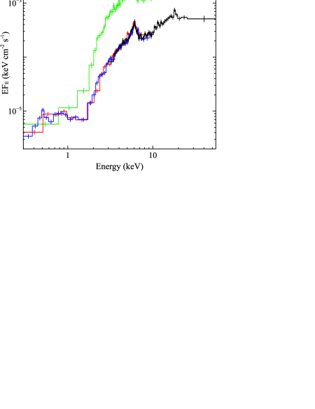
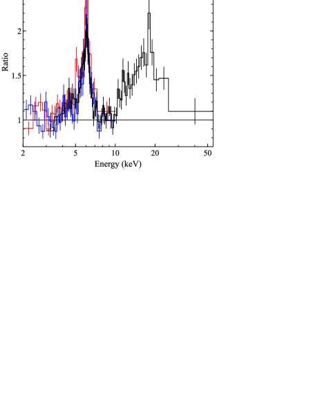
Figure 1: Left panel: the time-averaged XMM-Newton+NuSTAR spectrum from our 2017 observation of IRAS 00521–7054, unfolded through a model that is constant with energy. The NuSTAR FPMA+B data are shown in black, and the XMM-Newton EPIC-pn and EPIC-MOS data are shown in blue and red, respectively. For comparison, we also show the EPIC-pn data from 2006 (analysed in Tan et al. 2012) in green. Right panel: residuals to a simple CUTOFFPL continuum, modified by a partially covering neutral absorber, and applied to the 2017 data over the 2–3.5, 7–10 and 40–55 keV energy ranges. The key signatures of relativistic disc reflection, i.e. a broadened iron line at $\sim$6 keV and a strong Compton hump at $\sim$20 keV, are seen. The data in both panels have been rebinned for visual purposes.

2 Observations and Data Reduction

NuSTAR and XMM-Newton performed coordinated observations IRAS 00521–7054 in 2017; a summary of the observations is given in Table 1. The bulk of the NuSTAR exposure was taken contemporaneously with XMM-Newton in September/October, but owing to scheduling constraints the final segment was taken $\sim$6 weeks later. The average source flux varied by $<$10% in the 3–50 keV band (see below) between the NuSTAR exposures, and none of the individual XMM-Newton or NuSTAR exposures show notable variability on intra-observational timescales, so we treat all of the data as a single observation despite this separation and extract a single, time-averaged broadband spectrum.

We reduced the NuSTAR data as standard using the NuSTAR Data Analysis Software (NUSTARDAS) v1.8.0 and instrumental calibration files from caldb v20180312. We cleaned the unfiltered event files with NUPIPELINE using the standard depth correction, which significantly reduces the internal high-energy background, and also excluded passages through the South Atlantic Anomaly (using the following settings: SAACALC = 3, SAAMODE = Optimized and TENTACLE = yes). Source products and instrumental responses were extracted from circular regions of radius 50^′′ using NUPRODUCTS for both of the focal plane modules (FPMA/B), and background was estimated from larger regions of blank sky on the same detector as IRAS 00521–7054. In order to maximise the exposure, in addition to the standard ‘science’ (mode 1) data, we also extracted the ‘spacecraft science’ (mode 6) data following the procedure outlined in Walton et al. (2016b). For these observations of IRAS 00521–7054, the mode 6 data provide $\sim$33% of the total $\sim$400 ks good NuSTAR exposure. As the source is relatively faint during this epoch (see below), we combined the data from the FPMA and FPMB modules into a single spectrum using ADDASCASPEC, and fit the NuSTAR data over the $\sim$3–50 keV band, above which the background dominates.

The data reduction for the XMM-Newton data was also carried out following standard procedures. We used the XMM-Newton Science Analysis System (SAS v15.0.0) to clean the raw observation files, specifically using EPCHAIN and EMCHAIN for the EPIC-pn detector (Strüder et al. 2001) and the two EPIC-MOS units (Turner et al. 2001), respectively. Source products were then extracted from the cleaned event files from circular regions of radius 25^′′ using XMMSELECT, and background was again estimated from larger regions of blank sky on the same detector chips as IRAS 00521–7054. These XMM-Newton observations suffered from reasonably extensive periods of background flaring, so we utilized the method outlined in Piconcelli et al. (2004) to determine the level of background emission that maximises the signal-to-noise (S/N) for the source for a given energy band; as we are primarily interested in the direct emission from the AGN, we maximise the S/N in the 5–10 keV band. As recommended, we only extracted single and double patterned events for EPIC-pn (PATTERN $\leq$ 4) and single to quadruple patterned events for EPIC-MOS (PATTERN $\leq$ 12), and instrumental response files for each of the detectors were generated using RMFGEN and ARFGEN. We note that the observed count rates were sufficiently low that pile-up is of no concern ($\sim$0.06 $\rm\thinspace ct~{}s^{-1}$ and $\sim$0.02 $\rm\thinspace ct~{}s^{-1}$ for EPIC-pn and each EPIC-MOS unit, respectively). After performing the reduction separately for the two EPIC-MOS units, we also combined these data into a single spectrum using ADDASCASPEC. We fit the XMM-Newton data over the full 0.3–10 keV band.

Table 1: Details of the 2017 X-ray observations of IRAS 00521-7054.

Mission	OBSID	Start Date	Exposure (ks)[a]
XMM-Newton	0790590101	2017-09-30	65/101
	0795630201	2017-10-02	55/65
NuSTAR	60301029002	2017-09-30	106
	60301029004	2017-10-02	184
	60301029006	2017-11-17	111

^a XMM-Newton exposures are listed for the EPIC-pn/MOS detectors, after correcting for background flaring.

3 Spectral Analysis

We focus on a spectral analysis of the broadband XMM-Newton+NuSTAR data, using XSPEC  v12.6.0f (Arnaud 1996) to model the data. Uncertainties on the spectral parameters are quoted at the 90% confidence level for a single parameter of interest. Each of the datasets are rebinned to have a minimum S/N of 5 per bin, sufficient for $\chi^{2}$ minimisation. All of our models include a neutral absorber associated with our own Galaxy, modelled with the TBABS neutral absorption code (Wilms et al. 2000). As recommended we use the cross-sections of Verner et al. (1996) for the neutral absorption, but we adopt the solar abundance set of Grevesse & Sauval (1998) for self-consistency with both the XILLVER reflection models (García & Kallman 2010) and the XSTAR photoionisation code (Kallman & Bautista 2001), as these are used to model the central AGN throughout this work. The column density of the Galactic absorption component is fixed the to $N_{\rm{H,Gal}}=5.26\times 10^{20}$ $\rm\thinspace cm^{-2}$ (Kalberla et al. 2005). As is standard, cross-calibration uncertainties between the different detectors are accounted for by allowing multiplicative constants to vary between them. We fix EPIC-pn at unity, and the others are found to be within $\sim$10% of unity, as expected (Madsen et al. 2015).

The broadband spectrum is shown in Figure 1 (left panel), along with the previous XMM-Newton data obtained in 2006 (see Tan et al. 2012) for comparison. The data above $\sim$2 keV, where the direct emission from the central nucleus dominates, shows that IRAS 00521–7054 was significantly fainter during our 2017 observations than the previous X-ray observations with XMM-Newton and Suzaku (the 2013 Suzaku observation caught the source in the same flux state as the 2006 XMM-Newton observations; Ricci et al. 2014). The observed 2–10 keV flux in 2017 is $\sim$4 $\times 10^{-13}$ $\rm\thinspace erg~{}cm^{-2}~{}s^{-1}$, a factor of $\sim$6 fainter than the previous XMM-Newton and Suzaku observations. Despite this, at the lowest energies (below $\sim$1 keV) the 2006 and 2017 data show similar fluxes, implying that these energies are dominated by diffuse plasmas and scattered emission, similar to other obscured AGN (e.g. Winter et al. 2009; Walton et al. 2018a).

To further highlight the features in the high-energy spectrum we also show the data/model ratio of the combined XMM-Newton+NuSTAR data above 2 keV to a simple absorbed CUTOFFPL continuum, fit to the 2–3.5, 7–10 and 40–55 keV bands (observed frame) where the primary AGN continuum would be expected to dominate (Figure 1, right panel). We allow the absorption to be partially covering, but find a covering factor of $C_{\rm{f}}\sim 1$, along with a column density of $N_{\rm{H}}\sim 7\times 10^{22}$ $\rm\thinspace cm^{-2}$, a photon index of $\Gamma\sim 1.6$ and a cutoff energy of $E_{\rm{cut}}\sim 170$ keV. A strong, broad emission feature is clearly seen in the iron bandpass, similar to the broad iron K emission previously reported for this source (Tan et al. 2012; Ricci et al. 2014), and a strong excess of emission is also seen above 10 keV. This high-energy excess peaks at $\sim$20 keV, as expected for a Compton reflection continuum. In addition to these features, a narrower core to the iron emission at 6.4 keV is clearly visible.

Interestingly, the column density we find when using this simple model is similar to the neutral columns inferred with similar models in both Tan et al. (2012) and Ricci et al. (2014) ($\sim$6 and $\sim$7 $\times 10^{22}$ $\rm\thinspace cm^{-2}$, respectively), suggesting that the low flux observed here is not related to strong changes in the line-of-sight absorption. Instead, the flux variability is likely intrinsic to the source, and related to changes in the accretion rate through the inner regions of the disc.

3.1 Broadband Continuum Modeling (Model 1)

We construct a model for the broadband continuum consisting of the primary Comptonised X-ray continuum, relativistic reflection from the inner accretion disc to account for the broad iron emission, a partially covering neutral absorber associated with the nucleus and a fully covering neutral absorber to account for the galaxy-scale column in the IRAS 00521–7054 galaxy (similar to the Galactic column), a more distant reflector to account for the narrower iron emission, and a collisionally ionised plasma to additionally account for the constant soft X-ray emission. Both of the neutral absorbers associated with IRAS 00521–7054 are again modeled with the TBABS absorption code, and are assumed to be at the redshift of the host-galaxy. Relaxing this assumption for the nuclear absorber (refered to as TBABS₂) does not improve the fit, and the X-ray constraints on the absorber redshift are consistent with that of the host galaxy. This absorption component is allowed to be partially covering to account for the weak scattered nuclear emission ubiquitously seen in the soft X-ray band (in addition to ionized plasma emission) in absorbed AGN (e.g. Winter et al. 2009). The nuclear absorber only acts on the direct emission from the central nucleus (the primary X-ray continuum and the relativistic disc reflection), while both of the absorbers associated with the galaxy-scale absorption in IRAS 00521–7054 (TBABS₁) and our own Galaxy (TBABS_Gal) act on all model components.

For the relativistic reflection, we use the RELXILLLP_CP model (v1.2.0; García et al. 2014). This accounts for both the continuum emission from the illuminating X-ray source (assuming an NTHCOMP continuum, parameterised by a photon index, $\Gamma$, and the electron temperature, $kT_{\rm{e}}$; Zdziarski et al. 1996; Zycki et al. 1999) and the reflected emission from the accretion disc. The disc reflection contribution is computed self-consistently assuming a simple lamppost geometry with a thin disc, both in terms of the emissivity profile of the disk and the strength of the reflected emission (the reflection fraction, $R_{\rm{frac}}$; see Dauser et al. 2016). We assume that the inner accretion disc reaches the innermost stable circular orbit (ISCO) in all our analysis, and fix the outer disk to the maximum value allowed by the model (1000 $R_{\rm{G}}$), so both the emissivity profile and the reflection fraction are set by the dimensionless spin of the black hole, $a$, and the height of the illuminating X-ray source, $h$. The height of the corona is fit in units of the vertical horizon radius to ensure that the X-ray source is always outside this point, but where relevant we convert this to units of $R_{\rm{G}}$ when quoting the results. The other key free parameters are the inclination, the ionisation parameter, and the iron abundance of the disk ($i$, $\xi$ and $A_{\rm{Fe}}$, respectively; the rest of the cosmically abundant elements are assumed to have solar abundances). The ionisation parameter is defined as $\xi=L_{\rm{ion}}/nR^{2}$, where $L_{\rm{ion}}$ is the ionising luminosity (assessed between 1–1000 Ry), $n$ is the density of the material, and $R$ is the distance between the material and the ionising source.

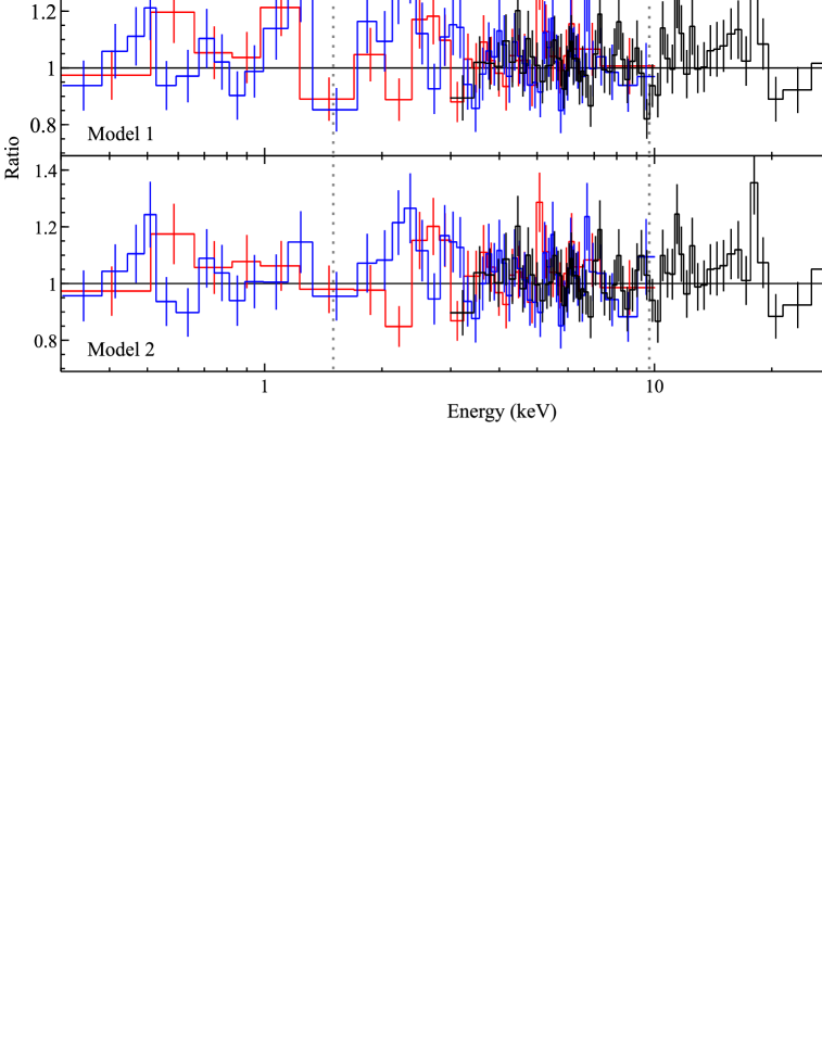
Figure 2: Data/model ratios for our baseline broadband continuum model (Model 1, see Section 3.1), and the model including strongly blueshifted ionised absorption (Model 2, see Section 3.2). The NuSTAR and XMM-Newton data are shown in the same colours as in Figure 1, and the data have again been rebinned for visual clarity. The vertical dotted lines show the approximate energies of the main features of the ionised, blueshifted absorber.

For the more distant reflection we use the XILLVER_CP model (configured such that this component only provides a reflection spectrum), as this also assumes an NTHCOMP ionising continuum. Although this implicitly assumes a slab geometry for the distant reflector, and the true geometry may more closely resemble an equatorial torus, our recent work on the absorbed AGN in IRAS 13197-1627 found that similar results were obtained regardless of the geometry assumed for the distant reflector (Walton et al. 2018a). XILLVER_CP shares most of its key free parameters with the RELXILLLP_CP model (aside from those associated with the relativistic blurring), and we assume that the distant reflector is neutral. While the core of the iron emission is clearly narrower than the relativistic emission, modeling it with a simple Gaussian profile suggests this emission does still have some width ($\sigma\sim 0.18$ keV). This is consistent with the results presented by Gandhi et al. (2015), who find that the majority of the narrow core of the iron emission in Seyfert galaxies arises from scales interior to the dust sublimation radius, and is likely associated with the broad line region (see also Miller et al. 2018). We therefore assume the line width here arises due to velocity broadening, so we convolve the XILLVER component with a Gaussian kernel (GSMOOTH) which has a constant ratio of $\sigma/E$; the width of this Gaussian kernel is evaluated at 6 keV. Finally, we account for the distant plasma emission with a MEKAL model. The formal model expression is as follows: TBABS${}_{\rm{Gal}}\times$TBABS${}_{1}\times$ (GSMOOTH$\otimes$XILLVER_CP + MEKAL + TBABS${}_{2}\times$RELXILLLP_CP).

Table 2: Results obtained for the free parameters in the lamppost reflection models fit to the broadband XMM-Newton+NuSTAR data for IRAS 00521–7054.

Model Component	Parameter		Model
			1	2
TBABS1 (galaxy-scale)	$N_{\rm{H,1}}$	[$10^{20}$ cm-2]	$<6.2$	$4.5^{+3.5}_{-4.1}$
TBABS2 (nuclear)	$N_{\rm{H,2}}$	[$10^{22}$ cm-2]	$6.8^{+2.2}_{-0.4}$	$6.7^{+2.2}_{-0.6}$
	$C_{\rm{f,2}}$	[%]	$96.4^{+1.6}_{-0.7}$	$96.3^{+0.7}_{-1.7}$
RELXILLLP_CP	$\Gamma$		$1.96^{+0.06}_{-0.09}$	$1.91^{+0.10}_{-0.17}$
	$kT_{\rm{e}}$[a]	[keV]	$36^{+12}_{-21}$	$43^{+24}_{-32}$
	$a$		$>0.73$	$>0.77$
	$i$	[∘]	$63^{+3}_{-27}$	$59^{+3}_{-16}$
	$h$	[$R_{\rm{G}}$]	$<7$	$<5$
	$R_{\rm{frac}}$[b]		$>1.6$	$>1.7$
	$\log\xi$	$\log$[erg cm s-1]	$1.1^{+1.9}_{-0.8}$	$2.1^{+0.4}_{-2.0}$
	$A_{\rm{Fe}}$[c]	[solar]	$3.1^{+0.4}_{-1.6}$	$3.2^{+0.6}_{-0.9}$
	$\log[\rm{Norm}]$		$-3.69^{+0.34}_{-1.88}$	$-3.32^{+0.22}_{-1.98}$
XSTAR	$\log\xi$	$\log$[erg cm s-1]	–	$4.7\pm 0.1$
	$N_{\rm H}$	[$10^{22}$ cm-2]	–	$2.8^{+1.7}_{-1.1}$
	$z_{\rm{abs}}$		–	$-0.349\pm 0.009$
XILLVER_CP	$\sigma$ (at 6 keV)	[keV]	$0.19^{+0.06}_{-0.05}$	$0.20\pm 0.06$
	Norm	[$10^{-6}$]	$4.3^{+1.4}_{-0.7}$	$4.4^{+1.1}_{-0.8}$
MEKAL	$kT$	[keV]	$0.76^{+0.06}_{-0.11}$	$0.79^{+0.09}_{-0.10}$
	Norm	[$10^{-6}$]	$1.5^{+1.4}_{-0.4}$	$1.1^{+0.7}_{-0.4}$
$\chi^{2}$/DoF			621/553	585/550

For self-consistency within our model, we make sure to link the iron abundance parameters across all the different model components associated with IRAS 00521–7054, and we also assume their abundances for the other cosmically abundant elements are solar. We also link the photon index between the RELXILLLP_CP and XILLVER_CP components. However, in the later versions of RELXILL (v1.0.4 onwards) the electron temperature is given in the rest-frame of the X-ray source for the lamppost models, prior to any gravitational redshift ($z_{\rm{grav}}$) that should be applied to the emission as seen by a distant observer. As such, we apply this redshift to the rest-frame electron temperature when determining the illuminating spectrum seen by the distant reflector. This depends on both the spin of the black hole ($a$) and the height of the X-ray source ($h$; here in units of $R_{\rm{G}}$) following equation 1.

$$(1+z_{\rm{grav}})=\bigg{(}1-\frac{2h}{h^{2}+a^{2}}\bigg{)}^{-\frac{1}{2}}$$ (1)

This model (which we refer to as Model 1) describes the broadband spectral shape of IRAS 00521–7054 well, with $\chi^{2}$ = 621 for 553 degrees of freedom (DoF). The best-fit parameters are given in Table 2, and we show the data/model ratio in Figure 2 (top panel). Even when allowing for partially covering absorption, the data prefer a large reflection fraction of $R_{\rm{frac}}$ $>$ 1.6. This requires strong gravitational lightbending for a standard thin accretion disc (which would otherwise give $R_{\rm{frac}}$ $\sim$ 1). In turn, this requires both a rapidly rotating black hole and a relatively compact illuminating corona (Miniutti & Fabian 2004; Dauser et al. 2016), and we find $a>0.73$ and $h<7$ $R_{\rm{G}}$. Our results also imply that IRAS 00521–7054 has a super-solar iron abundance ($A_{\rm{Fe}}\sim 3$), and that we view the accretion disk at a moderately high inclination ($i\sim 60$^∘). We stress that, with the exception of the galaxy-scale absorber associated with IRAS 00521–7054, the removal of any of the broadband continuum components included in this model significantly degrades the fit, increasing the $\chi^{2}$ by $\geq$8 per free parameter. The galaxy-scale absorber is not formally required by the data (hence only an upper limit on the column is obtained). However, we retain this component in our final model to account for more realistic errors on the photon index, which is influenced in part by the slope of the spectrum at the lowest energies ($\lesssim$1 keV) where the scattered continuum contributes.

3.2 Ionised Absorption (Model 2)

Although Model 1 describes the broadband continuum well, the NuSTAR data show evidence for an absorption feature at $\sim$9.5 keV in the observed frame. There are no known instrumental features close to this energy. Adding a Gaussian absorption feature provides a reasonable improvement of $\Delta\chi^{2}=14$ for three additional free parameters, and we find a rest-frame line energy of $E=10.1^{+0.2}_{-0.1}$ keV, a line width of $\sigma<0.6$ keV (corresponding to a velocity broadening of $\lesssim 18,000$ $\rm\thinspace km~{}s^{-1}$), and an equivalent width of $120^{+180}_{-50}$ eV. Given the systemic redhift of IRAS 00521–7054, the line energy implies a blueshift of either $z_{\rm{abs}}\sim 0.31$ or 0.34 relative to the cosmological redshift of IRAS 00521–7054, assuming an association with Fe XXVI or Fe XXV, respectively, either of which would place the absorber firmly in the ‘ultrafast’ outflow (UFO) category (e.g. Tombesi et al. 2010b, a; Gofford et al. 2013; Nardini et al. 2015; Matzeu et al. 2017; Parker et al. 2018), and would even make it one of the most extreme in terms of the observed blueshift.

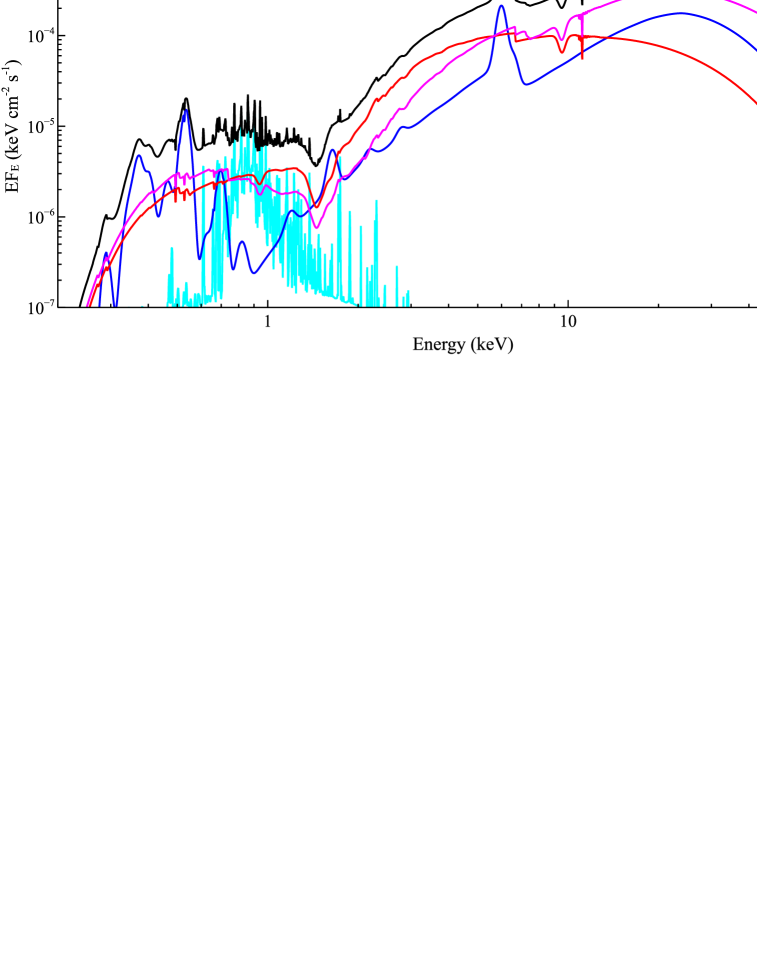
Figure 3: The relative contributions of the different components for our final model including the highly blueshifted ionized absorption (Model 2). The total model is shown in black, the Comptonised continuum in red, the relativistic disc reflection in magenta, the distant reflection in blue, and the distant plasma in cyan.

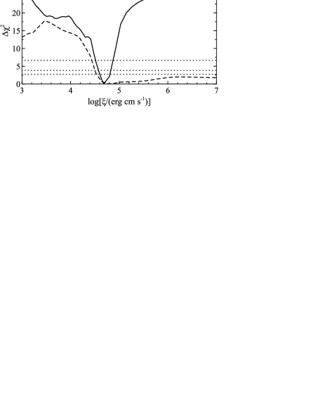
Figure 4: The $\Delta$$\chi^{2}$ confidence contours for the blueshift (left panel, given in the rest frame of IRAS 00521–7054) and the ionisation parameter (right panel) of the highly ionised absorber. The horizontal dotted lines represent the 90, 95 and 99% confidence levels for a single parameter of interest. The solid curves show the confidence contours for the full dataset, and the dashed curves show the contours after excluding the 1.25–1.65 keV energy range to cut out the feature at $\sim$1.5 keV.

To investigate this further we replace the Gaussian absorption line with a physical photoionisation model using XSTAR. We use a grid of absorption models with the ionisation parameter, column density and iron abundance as free parameters. All other elements have solar abundances, and these absorption models also assume a velocity broadening of 10,000 $\rm\thinspace km~{}s^{-1}$ (through the ‘turbulent’ velocity parameter in XSTAR; $v_{\rm{turb}}$), based on the constraints above and the line broadening seen in other well-studied UFO sources (e.g. Pounds et al. 2003; Nardini et al. 2015). During our analysis, the iron abundance is linked to that of the continuum model components, and as with the neutral absorbers, this absorption component is only applied to the direct emission from the central nucleus (the RELXILLLP_CP component), such that the model expression is updated to the following: TBABS${}_{\rm{Gal}}\times$TBABS${}_{1}\times$(GSMOOTH$\otimes$XILLVER_CP + MEKAL + TBABS${}_{2}\times$XSTAR$\times$ RELXILLLP_CP).

Since the ionisation parameter is defined using the ionising luminosity across the 1–1000 Ry bandpass, the intrinsic broadband (optical to X-ray) spectral energy distribution (SED) actually plays an important role in setting the ionisation parameter at which highly ionised iron transitions are observed. We therefore inspected the data from the Optical Monitor on board XMM-Newton (Mason et al. 2001), which took exposures in each of its optical–UV filters (V, B, U, UVM2, UVW1 and UVW2). However, while IRAS 00521–7054 is clearly detected in each of these filters, in almost all cases the OM data show an extended counterpart, implying a non-negligible contribution from the host galaxy. Given this, and the fairly heavy obscuration towards the nucleus, we conclude that it is beyond the scope of this work to observationally determine the intrinsic SED for the central AGN for use with XSTAR. Instead, we take a simpler approach, and for the input to XSTAR we assume an SED in which the X-ray emission is dominated by Comptonisation, and the optical/UV emission is dominated by a standard accretion disc (Shakura & Sunyaev 1973). The X-ray continuum is modeled with NTHCOMP, with the spectral parameters ($\Gamma$, $kT_{\rm{e}}$) set by the continuum analysis above, and the accretion disk is modeled with DISKBB (Mitsuda et al. 1984). To set the disc temperature, based on the arguments in Ricci et al. (2014) we assume that IRAS 00521–7054 is accreting at roughly its Eddington rate during the higher flux observations in the archive. Adopting a bolometric correction for the 2–10 keV band of $\kappa_{2-10}\equiv L_{2-10}/L_{\rm{bol}}=150$ – as appropriate for high-Eddington sources (Vasudevan & Fabian 2009; Lusso et al. 2010) – implies an intrinsic bolometric luminosity of $L_{\rm{bol}}\sim 6\times 10^{45}$ erg s^-1 during these epochs (Tan et al. 2012), given the luminosity distance of 300 Mpc (based on a standard cosmology with $H_{0}$ = 73 km s^-1 Mpc^-1, $\Omega_{\rm{matter}}=0.27$ and $\Omega_{\rm{vacuum}}=0.73$). In turn, this implies a black hole mass of $M_{\rm{BH}}\sim 5\times 10^{7}$ $\rm M_{\odot}$, and therefore an inner disc temperature of $T_{\rm{in}}\sim 0.05$ keV. Finally, we set the normalisation of the disc relative to the X-ray continuum to give the same bolometric correction as above.

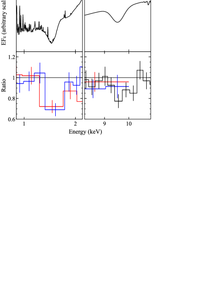
Figure 5: Zoom-in around the key absorption features for the best-fit XSTAR model (Model 2, shown in full in Figure 3; top panels) and the data/model ratios after the XSTAR component has been removed (without refitting; bottom panels). The left panels focus on the feature at $\sim$1.5 keV, and the right panels focus on the feature at $\sim$9.5 keV. For the model plots, we only show the total model (rather than the individual components) for clarity, and the colours in the ratio plots have the same meaning as in Figures 1 and 2.

The inclusion of the photoionised absorber provides a much larger improvement to our baseline continuum model than the single Gaussian absorption line, with $\Delta\chi^{2}=36$ for three additional free parameters. We refer to this as Model 2 and, given the level of improvement, consider this our preferred model (see Section 3.2.1 for a formal assessment of the significance of this outflow); the best-fit parameter values are given in Table 2, the data/model ratio for the fit is shown in Figure 2 (bottom panel), and we show the relative contributions of the different components for this model in Figure 3. Figure 4 shows the confidence contours for both the blueshfit (relative to the cosmological redshift of IRAS 00521–7054) and the ionisation parameter of the ionised absorber (solid lines); the data clearly prefer the Fe XXV solution (which corresponds to $z_{\rm{abs}}\sim 0.35$) over the Fe XXVI solution (which would have $z_{\rm{abs}}\sim 0.31$). This is because, with the Fe XXV solution, the photoionised absorber is also able to match a second absorption feature at $\sim$1.5 keV (observed frame) in addition to the high-energy feature at $\sim$9.5 keV (see Figure 2, and also Figure 5 where we show a zoom-in on these two features). This $\sim$1.5 keV feature is also produced by iron in the model, in this case the complex of L-shell transitions from Fe XXI-XXIV, which matches the observed line energy for the same blueshift as the Fe XXV solution for the line observed at 9.5 keV, resulting in a much stronger total statistical improvement than the single Gaussian. Accounting for the relativistic corrections necessary for such extreme blueshifts, we find the line-of-sight velocity of the absorber to be $\beta_{\rm{LoS}}=v_{\rm{LoS}}/c=-0.405\pm 0.012$.

Given the presence of a photoionised absorber, we also test for the presence of associated photoionised emission. We again use XSTAR, assuming the same input continuum, ionisation state, column density and iron abundance as the absorber. The emitter is placed at the redshift of IRAS 00521–7054, and we crudely attempt to account for the expected broadening for a diverging outflow based on the observed outflow velocity using another Gaussian smoothing kernel. However, we find that the data are not sensitive to this emission; adding such a component provides a negligible improvement in the fit ($\Delta\chi^{2}<1$), and so we do not include this in our final model. In principle the normalisation of the XSTAR emission component, $\kappa$, can be used to determine the solid angle subtended by the wind, as $\Omega=\kappa D_{\rm{kpc}}/L_{38}$, where $\Omega$ is the solid angle (normalised by $4\pi$ such that $0\leq\Omega\leq 1$), $D_{\rm{kpc}}$ is the distance in kpc, and $L_{38}$ is the ionising luminosity in units of $10^{38}$ erg s^-1 (csee e.g. Reeves et al. 2018a). However, taking the values for $D_{\rm{kpc}}$ and $L_{38}$ discussed above, in this case the limits the current data can place on the normalisation are sufficiently weak that $\Omega$ is completely unconstrained.

Figure 6: The $\Delta$$\chi^{2}$ confidence contours for the spin parameter from our preferred model for the broadband data of IRAS 00521–7054 (Model 2, see Section 3.2). We show contours computed with the electron temperature free to vary (solid line) and assuming a temperature of $kT_{\rm{e}}=40$ keV (dashed line). The horizontal dotted lines represent the 90, 95 and 99% confidence levels for a single parameter of interest.

The key continuum parameters are all consistent with the values obtained in Model 1, and the constraints are generally similar. Again we find the model prefers a large reflection fraction, and thus a rapidly rotating black hole ($a>0.77$). We show the confidence contour for the black hole spin in Figure 6; although a high spin is preferred, the level at which a non-rotating black hole is excluded is not particularly strong. However, it is worth noting that the best-fit solutions at low spin also require a very low temperature for the corona of $kT_{\rm{e}}\sim 10$ keV. This is because of the complex interplay that exists between some of the main continuum parameters in our model; the electron temperature is degenerate with both the black hole spin and, in particular, the height of the corona. This is because the temperature is assessed in the rest-frame of the X-ray source (rather than the observed frame) and these parameters set the gravitational redshift (Equation 1). We show a 2-D confidence contour showing the degeneracy between $h$ and $kT_{\rm{e}}$ in Figure 7. This degeneracy exists down to the point at which, in the limit of negligible gravitational redshift, the temperature becomes too low to produce the observed hard X-ray flux, at which point the fit quickly degrades. While coronae with low temperatures have been reported in a few rare cases (Tortosa et al. 2017; Kara et al. 2017), intrinsic temperatures are typically $kT_{\rm{e}}\sim 40-50$ keV (even after correcting approximately for gravitational redshift; Fabian et al. 2015), similar to the best-fit value found here. We therefore also re-compute the confidence contour for the spin with the electron temperature fixed to $kT_{\rm{e}}=40$ keV, which we also show in Figure 6 (dashed line). Unsurprisingly, the constraint on the spin is much tighter ($a>0.91$; repeating this analysis with Model 1 also gives similar results). This is because the model is now unable to lower the electron temperature when in regions of parameter space in which the gravitational redshift would be weaker (lower $a$, higher $h$) to reproduce the strong curvature observed above $\sim$10 keV, and thus the preference for a large reflection fraction – and in turn a high spin – is even stronger.

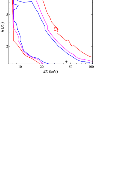
Figure 7: 2D confidence contours for $h$ and $kT_{\rm{e}}$ for IRAS 00521–7054 (using Model 2). The 90, 95 and 99% confidence contours for 2 parameters of interest are shown in blue, magenta and red, respectively. Note that here, $h$ is given in units of the vertical horizon radius, $R_{\rm{H}}$. A strong degeneracy is seen between these two parameters, as $kT_{\rm{e}}$ is given in the rest-frame of the X-ray source and $h$ plays an important role in setting the gravitational redshift (Equation 1). This degeneracy exists down to the temperature at which, in the limit of no gravitational redshift, the corona would be unable to reproduce the observed hard X-ray flux (which occurs at $kT_{\rm{e}}\sim 8$ keV).

3.2.1 Statistical Simulations

To formally test the statistical significance of the ionised outflow, we perform a series of spectral simulations. Using the same response and background files, and adopting the same exposure times and relative extraction areas as the real data used here, we simulated 10,000 sets of XMM-Newton (pn, combined MOS1 and MOS2) and NuSTAR (combined FPMA and FPMB) spectra with the FAKEIT command in XSPEC based on the best-fit model without the XSTAR grid (Model 1), allowing for independent Poisson fluctuations on both the simulated source and background spectra. Each of the simulated datasets was background subtracted and rebinned in the same manner as the real data, and analysed over the same bandpass. We initially fit each of the combined datasets with Model 1, before adding the XSTAR grid in order to determine the improvement in $\chi^{2}$ this extra model component provides by chance, linking the iron abundance to that of the other model components (as in our analysis of the real data). To account for the number of trials we scan the absorber velocity between $\beta_{\rm{LoS}}=0$ and 0.5 in 50 steps, and then run a full error scan on the key wind parameters for the best fit found to determine the maximum $\Delta\chi^{2}$ improvement provided. Of the 10,000 datasets simulated, none returned a chance improvement equivalent to or greater than that observed (at any velocity searched); we show the $\Delta\chi^{2}$ distribution in Figure 8. This implies that the outflow seen in the real data is significant at close to (or above) the 4$\sigma$ level (the low-number statistics associated with having no simulations that give a false positive mean the real probability could still be even larger). We stress that the simulations undertaken in this work also allow for a suitably complex continuum including reflection, as necessary to robustly determine the significance of the absorption (see the discussion in Zoghbi et al. 2015).

3.2.2 The Nature of the 1.5 keV Feature

Some caution may still be required, as the background for the XMM-Newton EPIC detectors is known to contain fluorescent emission from aluminium close in energy to the absorption feature inferred at $\sim$1.5 keV. In addition, this feature is also close in energy to the band in which the MEKAL plasma component, which includes line emission from a variety of different atomic species resulting in a complex low-energy spectrum, makes the strongest contribution. We therefore performed a variety of tests to determine whether the statistical detection of the ionised absorber could be driven by any of these issues, and investigate the potential nature of the $\sim$1.5 keV feature in more detail.

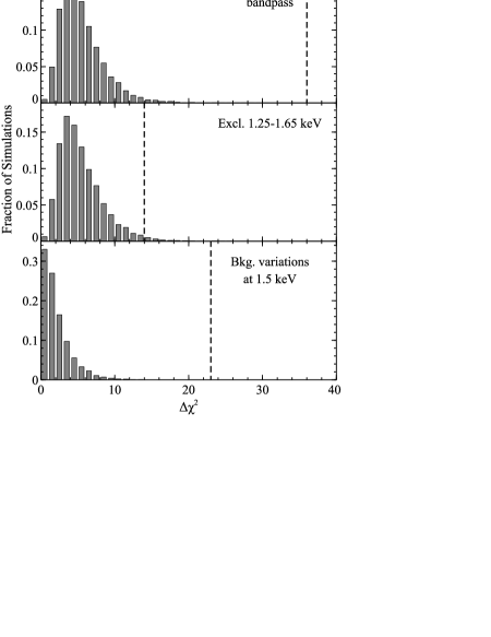
Figure 8: The $\Delta\chi^{2}$ distributions from our various analyses of the 10,000 simulations performed to assess the significance of the ultrafast outflow in IRAS 00521–7054. The top panel shows the analysis with the full bandpass for each simulation, the middle panel shows the analysis excluding the 1.25–1.65 keV energy range (testing the significance of just the Fe K absorption), and the bottom panel shows the analysis of the background variations at 1.5 keV (testing the nature of the Fe L absorption). In each case, the vertical dashed line shows the $\Delta\chi^{2}$ obtained with the real data for comparison.

First, to be conservative we also repeat our analysis on both the real and the simulated data after excluding the 1.25–1.65 keV energy range from the XMM-Newton detectors. We find that the addition of the XSTAR component improves the fit in the real data by $\Delta\chi^{2}=14$ for three additional free parameters (similar to the improvement provided by the single Gaussian line). The confidence contours for the blueshift and ionisation parameter of the absorber obtained with this analysis are also shown in Figure 4 (dashed lines). Unsurprisingly, in this case the fit cannot distinguish between the Fe XXV and Fe XXVI solutions without the lower-energy feature to help determine the ionisation parameter. Consequently, the range of allowed blueshifts is broader, but an extreme velocity is required regardless of whether the line is associated with Fe XXV or Fe XXVI. Similar re-analysis of the 10,000 simulated datasets finds that only 151 returned a chance improvement equivalent to or greater than that observed at any velocity searched after excluding this energy range, implying that the outflow is still detected at $\sim$98.5% significance regardless of the nature of the feature at $\sim$1.5 keV; the $\Delta\chi^{2}$ distribution obtained with this analysis is also shown in Figure 8.

Second, we consider whether there are likely to be any systematic issues regarding either our background subtraction or our modeling that could result in an artificial feature at $\sim$1.5 keV. To do so, we first varied the position of the background region, and found both the structure in the background-subtracted spectrum at $\sim$1.5 keV and the $\Delta\chi^{2}$ improvement provided by the ionised absorber to be insensitive to these variations. This is not surprising, as the spatial distrubition of the background aluminium emission across the XMM-Newton field of view is known to be stable. The same structure is also present if we adopt a more standard (and stricter) filtering of periods of high background (instead of using the method outlined in Piconcelli et al. 2004). The only systematic possibility that remains is that there is an error in the overall background level, and so we also repeated our analysis with a smaller XMM-Newton extraction region (for both EPIC-pn and EPIC-MOS), reducing the radius from 25^′′ to 20^′′. While this lowers the source counts by $\sim$5–10%, the background is reduced by $\sim$35%. Again, we find that the same structure is seen in the 1–2 keV band, and the statistical improvement provided by the addition of the ionised absorber is practically the same as that reported above, $\Delta\chi^{2}=35$. We also find no difference in the improvement provided by the ionised absorber if we allow the instrumental gain to vary for the XMM-Newton datasets.

We also tested whether the presence of this additional absorption feature was influenced by the parameters assumed for the MEKAL component. As discussed above, with the exception of iron (which is linked to the other model components and is free to vary), in our modeling we assume solar abundances for the elements included in the MEKAL model. However, since iron is found to have a non-solar abundance, it is also possible that this would also be the case for other elements, and given that a number of the elements included in MEKAL have lines close to $\sim$1.5 keV (e.g. magnesium and silicon), incorrectly assuming a solar abundance could potentially produce residuals consistent with an absorption feature in the EPIC data. To be conservative, we therefore repeated our fits allowing the abundances for all elements with atomic numbers between oxygen and calcium to vary between 0.1–10.0 times the solar value. We find that none of these abundances are well constrained (so we retain the assumption of solar abundances in the best-fit models presented), the structure in the 1–2 keV band is still seen, and that the statistical improvement provided by the ionised absorber is again similar to that reported above, $\Delta\chi^{2}=32$.

Finally, we also use our simualtions to assess the likelihood that the feature at $\sim$1.5 keV could be produced by a statistical fluctuation of the XMM-Newton aluminium background emission (although we note that the same basic structure is seen in the $\sim$1–2 keV energy range in both the EPIC-pn and EPIC-MOS data, which already implies that a pure statistical fluctuation is unlikely; see Figure 5). Modeling this feature with a Gaussian absorption line, we find an observed-frame energy of $1.51\pm 0.05$ keV and that the line is not well resolved ($\sigma<0.13$ keV), with an equivalent width of $130^{+90}_{-60}$ eV. The addition of this line improves the fit by $\Delta\chi^{2}=23$ in the real data (so this lower-energy features make a slightly stronger statistical contribution to the total improvement provided by the XSTAR grid). For each of our 10,000 simulations, we determine the $\Delta\chi^{2}$ improvement provided by a Gaussian feature with a similar energy and width (constrained to the ranges given above, since in this case we are testing for the effects of a background line at a known energy), but allowing for the feature to be in either absorption or emission (to reflect the fact that statistical fluctuations could be either positive or negative). Again, we find that none of the simulated datasets showed a chance improvement at or above the level seen in the real data; again, the $\Delta\chi^{2}$ distribution is shown in Figure 8. This implies that there is a $\lesssim$0.01% chance that a statistical fluctuation of the background aluminium line could produce a feature similar to that observed.

Based on these tests we therefore conclude that, although there is a background feature at a similar energy and the spectral model at low energies is complex, there is little evidence that the additional absorption feature seen in the source spectrum at $\sim$1.5 keV is purely the result of a poor background subtraction (either systematic or statistical) or an artefact of our modeling. We are therefore confident that our detection of a highly blueshifted, highly ionised absorber in IRAS 00521–7054 is robust.

4 Discussion

We have presented a spectral analysis of a deep, broadband X-ray observation of the Seyfert 2 galaxy IRAS 00521–7054, taken by XMM-Newton and NuSTAR in coordination. Although during this epoch the source was found to be significantly fainter than previous observations (by a factor of $\sim$6), the data still reveal that the X-ray spectrum of IRAS 00521–7054 is complex, showing contributions from relativistic disc reflection, absorption and additional reprocessing by more distant material, and ionised absorption from an ultrafast outflow. This complexity is analogous to the better-studied AGN in NGC 1365 (Risaliti et al. 2013; Walton et al. 2014; Rivers et al. 2015) and IRAS 13197–1627 (Miniutti et al. 2007; Walton et al. 2018a). The NuSTAR data presented here provide the first high-energy ($E>10$ keV) detection of this source, which is critical for disentangling the effects of these various processes.

4.1 The Inner Accretion Disc

From the relativistic reflection, we are able to place constraints on the key parameters for the innermost accretion flow. With regards to the black hole spin, we find that a rapidly rotating black hole is preferred ($a>0.77$; Figure 6), with tighter constraints if we assume a standard electron temperature of $kT_{\rm{e}}=40$ keV for the corona ($a>0.91$). This is a quantity of particular interest, as it provides a window into the growth history of the central supermassive black hole (e.g. Sesana et al. 2014; Dubois et al. 2014; Fiacconi et al. 2018). A high spin parameter implies the black hole primarily grew through a major phase of coherent accretion (perhaps triggered by a major merger or just through primarily feeding on gas in its host galaxy), as opposed to having a more chaotic growth history (e.g. growing through a large number of minor mergers). We also infer that we view the accretion disk at a relatively high inclination ($i=59^{+3}_{-16}$^∘), which is roughly consistent with its Seyfert 2 classification in the standard unified model for active galaxies (e.g. Antonucci 1993).

We stress that the spin constraint presented here is completely driven by the strength of the reflected emission, which is inferred to be high ($R_{\rm{frac}}>1.7$); if we remove the functional connection between the spin parameter and the reflection fraction, then we find the spin to be unconstrained. As such, our spin constraint is heavily dependent on the assumed thin disc geometry, which requires strong gravitational lightbending, and in turn a combination of a compact corona and a rapidly rotating black hole, to produce a large reflection fraction (Miniutti & Fabian 2004; Parker et al. 2014; Dauser et al. 2014). If the real geometry differs from this substantially, for example if the disc has a large scale height (as may be expected at high accretion rates relative to the Eddington limit; Shakura & Sunyaev 1973), then our spin constraint should be viewed with some caution. However, we note that the observation presented here caught IRAS 00521–7054 in a low-flux state (a factor of $\sim$6 fainter than prior X-ray osbervations). This does not appear to be related to large changes in the line-of-sight absorption, and may therefore imply a lower accretion rate through the inner disc than seen previously. Even if IRAS 00521–7054 was close to Eddington in its high-flux observations, the thin disc approximation may therefore still be reasonable during this epoch. Furthermore, the spin inferred here is consistent with the previous estimates presented by Tan et al. (2012) and Ricci et al. (2014), which also imply a rapidly rotating black hole with $a>0.73$ based solely on the profile of the iron emission; we note that the conditions seen in IRAS 00521–7054 (large reflection, compact corona) are the optimum conditions for obtaining spin constraints (Bonson & Gallo 2016; Kammoun et al. 2018). Although the line profile can also be influenced by these same issues relating to the assumed geometry, Taylor & Reynolds (2018) show that assuming the disc is thin when in reality it has some thickness tends to result in the spin being slightly underpredicted, so this should not change the consistency of the results. Nevertheless, an independent mass measurement for IRAS 00521–7054 is required to robustly determine its Eddington limit and thus its true accretion regime.

4.2 The Ultrafast Outflow

The other main result of interest is that we find strong evidence for an extremely rapid, ionised outflow. This imprints absorption features at $\sim$1.5 and $\sim$9.5 keV (observed frame) from ionised iron, which can be explained with a common blueshift of $z_{\rm{abs}}=-0.349\pm 0.009$ (relative to the cosmological redshift of IRAS 00521–7054) and an ionisation parameter of $\log[\xi/(\rm{erg~{}cm~{}s}^{-1})]=4.7\pm 0.1$ (see Figure 4). Applying the relativistic Doppler formula, we find a line-of-sight velocity of $\beta_{\rm{LoS}}=v_{\rm{LoS}}/c=-0.405\pm 0.012$. If this is associated with an outflow, this would be one of the most extreme outflows currently known in terms of its observed velocity; only PDS 456 is currently known to have a more blueshifted component to its outflow ($\beta_{\rm{out}}=0.46\pm 0.02$; Reeves et al. 2018b). Given the broadly equatorial geometry expected for winds from an accretion disc (e.g. Proga & Kallman 2004; Ponti et al. 2012), and the high inclination we infer from the reflected emission, it is likely that the true outflow velocity is close to that projected onto our line-of-sight, i.e. $\beta_{\rm{out}}\sim\beta_{\rm{LoS}}$.

The kinetic luminosity of the outflow, $L_{\rm{kin}}$ ($=1/2\dot{M}v_{\rm{out}}^{2}$), is given by Equation 2, based on the standard expression for $\dot{M}_{\rm{out}}$ for outflowing material derived by considering conservation of mass arguments:

$$L_{\rm{kin}}\approx 2{\pi}{\Omega}C_{\rm{V}}m_{\rm{p}}{\mu}nR^{2}v_{\rm{out}}^{3}$$ (2)

Here $C_{\rm{V}}$ is the volume filling factor of the wind (a measure of its ‘clumpiness’; normalised such that $0\leq C_{\rm{V}}\leq 1$, similar to $\Omega$), $m_{\rm{p}}$ is the proton mass, and $\mu$ is the mean atomic weight ($\sim$1.2 for solar abundances; given the super-solar iron abundance inferred $\mu$ may in reality be a little higher in this case).

The key question regarding AGN outflows is whether they carry sufficient power to drive the feedback invoked to explain known correlations between AGN and their host galaxies. This is usually determined by estimating the ratio between the kinetic power and the bolometric radiative luminosity. However, several of the quantities in Equation 2 are notoriously difficult to estimate: $n$, $R$, $\Omega$ and $C_{\rm{V}}$. In rare cases, it is possible to constrain some of these parameters directly (e.g. PDS 456; Nardini et al. 2015), but typically we are forced to re-frame Equation 2 in terms of quantities that are more readily observable. We can combine this with the defnition of the ionisation parameter to write an expression for $L_{\rm{kin}}/L_{\rm{bol}}$ in terms of $\xi$ (similar to, e.g., Pinto et al. 2016; Walton et al. 2016a; Kosec et al. 2018):

$$\frac{L_{\rm{kin}}}{L_{\rm{bol}}}\approx 2{\pi}m_{\rm{p}}\mu\frac{v_{\rm{out}}^{3}L_{\rm{ion}}}{{\xi}L_{\rm{bol}}}{\Omega}C_{\rm{V}}$$ (3)

Given the intrinsic SED adopted for IRAS 00521–7054 (see Section 3.2, we assume that the ratio $L_{\rm{ion}}/L_{\rm{bol}}\sim 1$. From the constraints on $v_{\rm{out}}$ and $\xi$, we therefore estimate that $L_{\rm{kin}}/L_{\rm{bol}}\sim 500\Omega C_{\rm{V}}$. Although we do not know either $\Omega$ or $C_{\rm{V}}$ here, the above $L_{\rm{kin}}/L_{\rm{bol}}$ estimate is comparable to similar calculations for the winds being seen in ultraluminous X-ray sources (ULXs; e.g. Pinto et al. 2016, 2017; Walton et al. 2016a; Kosec et al. 2018). These are now generally accepted to be high/super-Eddington accretors (e.g. Pintore et al. 2017; Koliopanos et al. 2017; Walton et al. 2018c, b), particularly after the discovery that some of these sources are powered by neutron stars (Bachetti et al. 2014; Fürst et al. 2016; Israel et al. 2017a, b; Carpano et al. 2018). This may further support the conclusions of Ricci et al. (2014) that, at least at its brightest, IRAS 00521–7054 is a high-Eddington source, around which we have based a number of our calculations.

This approach for estimating $L_{\rm{kin}}/L_{\rm{bol}}$ essentially assumes that all of the absorbing material is located at a single radius (i.e. $\Delta R\ll R$) that satisfies the definition of $\xi$, and should likely be considered an upper limit. Alternatively, we can use the fact that the column density is a line-of-sight integration of the density to write another expression for $L_{\rm{kin}}/L_{\rm{bol}}$ in terms of $N_{\rm{H}}$ adopting the opposite limiting geometry, i.e. $\Delta R\sim R$ (similar to, e.g., Krongold et al. 2007; Crenshaw & Kraemer 2012; Nardini et al. 2015):

$$\frac{L_{\rm{kin}}}{L_{\rm{bol}}}\approx 2{\pi}m_{\rm{p}}\mu\frac{RN_{\rm{H}}v_{\rm{out}}^{3}}{L_{\rm{bol}}}{\Omega}C_{\rm{V}}$$ (4)

Here we are still left with a factor of $R$, which is also not known. However, we can place a conservative lower limit on $R$ by equating the outflow velocity to the escape velocity (similar to Nardini & Zubovas 2018). For $v_{\rm{out}}=0.4c$, we find that $R>12.3$ $R_{\rm{G}}$, or $R\gtrsim 9\times 10^{11}$ m for our estimated black hole mass of $M_{\rm{BH}}\sim 5\times 10^{7}$ $\rm M_{\odot}$ (Section 3.2). From the constraints on $v_{\rm{out}}$ and $N_{\rm{H}}$, and taking $L_{\rm{bol}}\sim 10^{45}$ erg s^-1 for this epoch (based on the bolometric correction discussed in Section 3.2), we therefore estimate that $L_{\rm{kin}}/L_{\rm{bol}}\gtrsim 0.1\Omega C_{\rm{V}}$.

Although there are clearly still large uncertainties related to the geometry of the wind, unless the product $\Omega C_{\rm{V}}$ is small the ultra-fast outflow in IRAS 00521–7054 should easily be sufficient to drive AGN feedback on galactic scales (which requires $L_{\rm{kin}}$ to be greater than $\sim$a few % of $L_{\rm{bol}}$; Di Matteo et al. 2005; Hopkins & Elvis 2010), and may even dominate the total energy output from the system. We note that for PDS 456, the solid angle of the ultra-fast outflow is estimated to be $\Omega\sim 0.75$ (Nardini et al. 2015). Although the volume filling factor is still not formally known in that case, this must presumably also be large since the wind is persistently observed (Matzeu et al. 2017). Assuming IRAS 00521–7054 is close to is Eddington limit, as expected for PDS 456, it is plausible that its winds would be similar, also with a large solid angle. Nardini et al. (2015) also estimated the radius of the wind in PDS 456 to be $\sim$100 $R_{\rm{G}}$. Repeating the calculation above and assuming this radius and solid angle for IRAS 00521–7054, we infer $L_{\rm{kin}}/L_{\rm{bol}}\sim 0.6C_{\rm{V}}$.

The most extreme component of the PDS 456 outflow has only been seen when the source was in a low-flux state (Reeves et al. 2018b). This is also similar to the ultrafast outflow seen in the NLS1 IRAS 13224–3809, which produces significantly stronger absorption features when the flux is low (Parker et al. 2017; Pinto et al. 2018; Jiang et al. 2018), potentially related to the ionisation of the wind responding to changes in the source flux. Although we cannot currently address whether the strong outflow reported here would also be observable when IRAS 00521–7054 has a high flux, owing to a combination of S/N and bandpass issues with the available high-flux data, it is interesting to note that this has also been observed while the source was in a low-flux state, potentially similar to those better-studied cases (which are also high-Eddington accretors). Future broadband observations of IRAS 00521–7054 at higher fluxes will be needed to address this, and shed further light on the conditions in and/or the geometry of the wind.

Finally, we note that an alternative explanation for these highly blueshifted absorption features that does not require any kind of outflow has been proposed by Gallo & Fabian (2011, 2013), who suggest that they may arise through absorption in clouds suspended (potentially magnetically) above the disc, and co-rotating with it. This idea has recently been further explored by Fabian et al. (2018; submitted), and is primarily relevant for discs extending to the ISCO of a rapidly rotating black hole with very compact coronae (such that the illumination of the disc is strongly centrally concentrated and the contribution of the reflection to the observed spectrum is strong) and viewed at high inclination, broadly similar to the scenario inferred here. Such a configuration results in an apparent shift in the energy of the absorption line (rather than a broadening of it) as the reflected emission observed from the disc is almost completely dominated by the blue side, and so we only see absorption from material along this line-of-sight. Although velocities of up to 0.5$c$ are naturally present within the disc, the requirement that the absorbing medium be along our line-of-sight to the point of maximum emission likely sets an upper limit to the velocity shifts this model can reasonably produce that is lower than this. The velocity shift of $\beta_{\rm{LoS}}\sim 0.4$ inferred here is extreme and would likely push this interpretation to its limits, particularly given that the inclination is only moderately high, so an interpretation invoking an outflow (as discussed above) is likely preferred in this case.

5 Conclusions

The deep XMM-Newton+NuSTAR observation of IRAS 00521–7054 taken in 2017 shows evidence for relativistic reflection from the inner accretion disc, neutral absorption, further reprocessing by more distant material, and ionised absorption in an extreme, ultrafast outflow ($v_{\rm{out}}\sim 0.4c$). By modeling the disc reflection with simple lamppost models, we find that the central supermassive black hole is likely rapidly rotating ($a>0.77$), consistent with previous estimates from the profile of the relavitistic iron line. We also find that the accretion disc is viewed at a fairly high inclination ($i\sim 59$^∘). The energetics of the ultrafast outflow are still highly uncertain, but we estimate that it is likely sufficient to power galaxy-scale AGN feedback, and may even dominate the total energetics of the system.

References

- Antonucci (1993) Antonucci R., 1993, ARA&A, 31, 473
- Arnaud (1996) Arnaud K. A., 1996, in Astronomical Data Analysis Software and Systems V, edited by G. H. Jacoby & J. Barnes, vol. 101 of Astron. Soc. Pac. Conference Series, Astron. Soc. Pac., San Francisco, 17
- Bachetti et al. (2014) Bachetti M., Harrison F. A., Walton D. J., et al., 2014, Nat, 514, 202
- Baloković et al. (2018) Baloković M., Brightman M., Harrison F. A., et al., 2018, ApJ, 854, 42
- Bonson & Gallo (2016) Bonson K., Gallo L. C., 2016, MNRAS, 458, 1927
- Carpano et al. (2018) Carpano S., Haberl F., Maitra C., Vasilopoulos G., 2018, MNRAS, 476, L45
- Crenshaw & Kraemer (2012) Crenshaw D. M., Kraemer S. B., 2012, ApJ, 753, 75
- Dauser et al. (2014) Dauser T., García J., Parker M. L., Fabian A. C., Wilms J., 2014, MNRAS, 444, L100
- Dauser et al. (2016) Dauser T., García J., Walton D. J., et al., 2016, A&A, 590, A76
- Di Matteo et al. (2005) Di Matteo T., Springel V., Hernquist L., 2005, Nat, 433, 604
- Dubois et al. (2014) Dubois Y., Volonteri M., Silk J., 2014, MNRAS, 440, 1590
- Fabian et al. (2015) Fabian A. C., Lohfink A., Kara E., Parker M. L., Vasudevan R., Reynolds C. S., 2015, MNRAS, 451, 4375
- Fiacconi et al. (2018) Fiacconi D., Sijacki D., Pringle J. E., 2018, MNRAS
- Fürst et al. (2016) Fürst F., Walton D. J., Harrison F. A., et al., 2016, ApJ, 831, L14
- Gallo (2018) Gallo L. C., 2018, ArXiv 1807.09838
- Gallo & Fabian (2011) Gallo L. C., Fabian A. C., 2011, MNRAS, 418, L59
- Gallo & Fabian (2013) Gallo L. C., Fabian A. C., 2013, MNRAS, 434, L66
- Gandhi et al. (2015) Gandhi P., Hönig S. F., Kishimoto M., 2015, ApJ, 812, 113
- García et al. (2014) García J., Dauser T., Lohfink A., et al., 2014, ApJ, 782, 76
- García & Kallman (2010) García J., Kallman T. R., 2010, ApJ, 718, 695
- Gofford et al. (2013) Gofford J., Reeves J. N., Tombesi F., et al., 2013, MNRAS, 430, 60
- Grevesse & Sauval (1998) Grevesse N., Sauval A. J., 1998, Space Sci. Rev., 85, 161
- Harrison et al. (2013) Harrison F. A., Craig W. W., Christensen F. E., et al., 2013, ApJ, 770, 103
- Hopkins & Elvis (2010) Hopkins P. F., Elvis M., 2010, MNRAS, 401, 7
- Israel et al. (2017a) Israel G. L., Belfiore A., Stella L., et al., 2017a, Science, 355, 817
- Israel et al. (2017b) Israel G. L., Papitto A., Esposito P., et al., 2017b, MNRAS, 466, L48
- Jansen et al. (2001) Jansen F., Lumb D., Altieri B., et al., 2001, A&A, 365, L1
- Jiang et al. (2018) Jiang J., Parker M. L., Fabian A. C., et al., 2018, MNRAS
- Kalberla et al. (2005) Kalberla P. M. W., Burton W. B., Hartmann D., et al., 2005, A&A, 440, 775
- Kallman & Bautista (2001) Kallman T., Bautista M., 2001, ApJS, 133, 221
- Kammoun et al. (2018) Kammoun E. S., Nardini E., Risaliti G., 2018, A&A, 614, A44
- Kara et al. (2017) Kara E., García J. A., Lohfink A., et al., 2017, MNRAS, 468, 3489
- Koliopanos et al. (2017) Koliopanos F., Vasilopoulos G., Godet O., Bachetti M., Webb N. A., Barret D., 2017, A&A, 608, A47
- Kosec et al. (2018) Kosec P., Pinto C., Walton D. J., et al., 2018, MNRAS, 479, 3978
- Krongold et al. (2007) Krongold Y., Nicastro F., Elvis M., et al., 2007, ApJ, 659, 1022
- Lusso et al. (2010) Lusso E., Comastri A., Vignali C., et al., 2010, A&A, 512, A34
- Madsen et al. (2015) Madsen K. K., Harrison F. A., Markwardt C. B., et al., 2015, ApJS, 220, 8
- Mason et al. (2001) Mason K. O., Breeveld A., Much R., et al., 2001, A&A, 365, L36
- Matzeu et al. (2017) Matzeu G. A., Reeves J. N., Braito V., et al., 2017, MNRAS, 472, L15
- Miller et al. (2018) Miller J. M., Cackett E., Zoghbi A., et al., 2018, ApJ, 865, 97
- Miniutti & Fabian (2004) Miniutti G., Fabian A. C., 2004, MNRAS, 349, 1435
- Miniutti et al. (2007) Miniutti G., Ponti G., Dadina M., Cappi M., Malaguti G., 2007, MNRAS, 375, 227
- Mitsuda et al. (2007) Mitsuda K., Bautz M., Inoue H., et al., 2007, PASJ, 59, 1
- Mitsuda et al. (1984) Mitsuda K., Inoue H., Koyama K., et al., 1984, PASJ, 36, 741
- Nardini et al. (2015) Nardini E., Reeves J. N., Gofford J., et al., 2015, Science, 347, 860
- Nardini & Zubovas (2018) Nardini E., Zubovas K., 2018, MNRAS, 478, 2274
- Parker et al. (2018) Parker M. L., Buisson D. J. K., Jiang J., et al., 2018, MNRAS
- Parker et al. (2017) Parker M. L., Pinto C., Fabian A. C., et al., 2017, Nat, 543, 83
- Parker et al. (2014) Parker M. L., Wilkins D. R., Fabian A. C., et al., 2014, MNRAS, 443, 1723
- Piconcelli et al. (2004) Piconcelli E., Jimenez-Bailón E., Guainazzi M., Schartel N., Rodríguez-Pascual P. M., Santos-Lleó M., 2004, MNRAS, 351, 161
- Pinto et al. (2018) Pinto C., Alston W., Parker M. L., et al., 2018, MNRAS, 476, 1021
- Pinto et al. (2017) Pinto C., Alston W., Soria R., et al., 2017, MNRAS, 468, 2865
- Pinto et al. (2016) Pinto C., Middleton M. J., Fabian A. C., 2016, Nat, 533, 64
- Pintore et al. (2017) Pintore F., Zampieri L., Stella L., Wolter A., Mereghetti S., Israel G. L., 2017, ApJ, 836, 113
- Ponti et al. (2012) Ponti G., Fender R. P., Begelman M. C., Dunn R. J. H., Neilsen J., Coriat M., 2012, MNRAS, 422, L11
- Pounds et al. (2003) Pounds K. A., Reeves J. N., King A. R., Page K. L., O’Brien P. T., Turner M. J. L., 2003, MNRAS, 345, 705
- Proga & Kallman (2004) Proga D., Kallman T. R., 2004, ApJ, 616, 688
- Reeves et al. (2018a) Reeves J. N., Braito V., Nardini E., et al., 2018a, ApJ, 867, 38
- Reeves et al. (2018b) Reeves J. N., Braito V., Nardini E., Lobban A. P., Matzeu G. A., Costa M. T., 2018b, ApJ, 854, L8
- Reynolds (2014) Reynolds C. S., 2014, Space Sci. Rev., 183, 277
- Ricci et al. (2014) Ricci C., Tazaki F., Ueda Y., Paltani S., Boissay R., Terashima Y., 2014, ApJ, 795, 147
- Risaliti et al. (2013) Risaliti G., Harrison F. A., Madsen K. K., et al., 2013, Nat, 494, 449
- Rivers et al. (2015) Rivers E., Risaliti G., Walton D. J., et al., 2015, ApJ, 804, 107
- Sesana et al. (2014) Sesana A., Barausse E., Dotti M., Rossi E. M., 2014, ApJ, 794, 104
- Shakura & Sunyaev (1973) Shakura N. I., Sunyaev R. A., 1973, A&A, 24, 337
- Strüder et al. (2001) Strüder L., Briel U., Dennerl K., et al., 2001, A&A, 365, L18
- Tan et al. (2012) Tan Y., Wang J. X., Shu X. W., Zhou Y., 2012, ApJ, 747, L11
- Taylor & Reynolds (2018) Taylor C., Reynolds C. S., 2018, ApJ, 855, 120
- Tombesi et al. (2010a) Tombesi F., Cappi M., Reeves J. N., et al., 2010a, A&A, 521, A57
- Tombesi et al. (2010b) Tombesi F., Sambruna R. M., Reeves J. N., et al., 2010b, ApJ, 719, 700
- Tortosa et al. (2017) Tortosa A., Marinucci A., Matt G., et al., 2017, MNRAS, 466, 4193
- Turner et al. (2001) Turner M. J. L., Abbey A., Arnaud M., et al., 2001, A&A, 365, L27
- Vasudevan & Fabian (2009) Vasudevan R. V., Fabian A. C., 2009, MNRAS, 392, 1124
- Verner et al. (1996) Verner D. A., Ferland G. J., Korista K. T., Yakovlev D. G., 1996, ApJ, 465, 487
- Walton et al. (2018a) Walton D. J., Brightman M., Risaliti G., et al., 2018a, MNRAS, 473, 4377
- Walton et al. (2018b) Walton D. J., Fürst F., Harrison F. A., et al., 2018b, MNRAS, 473, 4360
- Walton et al. (2018c) Walton D. J., Fürst F., Heida M., et al., 2018c, ApJ, 856, 128
- Walton et al. (2016a) Walton D. J., Middleton M. J., Pinto C., et al., 2016a, ApJ, 826, L26
- Walton et al. (2013) Walton D. J., Nardini E., Fabian A. C., Gallo L. C., Reis R. C., 2013, MNRAS, 428, 2901
- Walton et al. (2014) Walton D. J., Risaliti G., Harrison F. A., et al., 2014, ApJ, 788, 76
- Walton et al. (2016b) Walton D. J., Tomsick J. A., Madsen K. K., et al., 2016b, ApJ, 826, 87
- Wilkins & Fabian (2012) Wilkins D. R., Fabian A. C., 2012, MNRAS, 424, 1284
- Wilms et al. (2000) Wilms J., Allen A., McCray R., 2000, ApJ, 542, 914
- Winter et al. (2009) Winter L. M., Mushotzky R. F., Reynolds C. S., Tueller J., 2009, ApJ, 690, 1322
- Zdziarski et al. (1996) Zdziarski A. A., Johnson W. N., Magdziarz P., 1996, MNRAS, 283, 193
- Zdziarski et al. (2003) Zdziarski A. A., Lubiński P., Gilfanov M., Revnivtsev M., 2003, MNRAS, 342, 355
- Zoghbi et al. (2015) Zoghbi A., Miller J. M., Walton D. J., et al., 2015, ApJ, 799, L24
- Zycki et al. (1999) Zycki P. T., Done C., Smith D. A., 1999, MNRAS, 309, 561