Quantum Teleportation-Inspired Algorithm for Sampling Large Random Quantum Circuits

Ming-Cheng Chen^1,2 cmc@ustc.edu.cn Riling Li³ Lin Gan^3,4 Xiaobo Zhu^1,2 Guangwen Yang^3,4 Chao-Yang Lu^1,2 cylu@ustc.edu.cn Jian-Wei Pan^1,2 pan@ustc.edu.cn ¹ Hefei National Laboratory for Physical Sciences at Microscale and Department of Modern Physics, University of Science and Technology of China, Hefei, Anhui 230026, China ² CAS Centre for Excellence and Synergetic Innovation Centre in Quantum Information and Quantum Physics, University of Science and Technology of China, Hefei, Anhui 230026, China. ³ Department of Computer Science & Technology, Tsinghua University, Beijing, China ⁴ National Supercomputing Center in Wuxi, China

(March 17, 2024)

Abstract

We show that low-depth random quantum circuits can be efficiently simulated by a quantum teleportation-inspired algorithm. By using logical qubits to redirect and teleport the quantum information in quantum circuits, the original circuits can be renormalized to new circuits with a smaller number of logical qubits. We demonstrate the algorithm to simulate several random quantum circuits, including 1D-chain $1000$ -qubit $42$ -depth, 2D-grid $125\times 8$ -qubit $42$ -depth and 2D-Bristlecone $72$ -qubit $32$ -depth circuits. Our results present a memory-efficient method with a clear physical picture to simulate low-depth random quantum circuits.

pacs:

Refer to caption — Figure 1: Quantum teleportation of multiple logical qubits for classical simulation of quantum circuits. (a) The circuit of quantum teleportation. Three physical qubits (black lines) in the quantum circuit are mimicked by one logical qubit (pink line). The logical qubit is used to redirect the flow of quantum information along the circuit topological structure. (b) The concept of transversal calculation for low-depth quantum circuits. Logical qubits are defined along the layers of two-qubit entangling gates. The number of logical qubits is proportional to the circuit depth. For a low-depth circuit, the number of logical qubits can be far less than physical qubits, therefore providing a memory-efficient classical simulation framework.

Information processing at quantum mechanics level has attracted great scientific interest since the development of quantum polynomial-time factoring algorithm and fault-tolerant quantum computing theory Nielsen . Many quantum algorithms are proposed to speed up solving important problems, such as solving linear system linear and complex molecular structure chemistry . Recently, high-fidelity quantum gates above fault-tolerance threshold have been demonstrated on superconducting qubits and trapped ions highfidelity1 ; highfidelity2 ; highfidelity3 . However, despite the great theoretical and experimental progress in the past two decades, these promising quantum algorithms still suffer from the lack of large-scale fault-tolerance quantum computing hardware or lack of strict proof of the computation complexity advantage.

The emerging quantum algorithms of Quantum Sampling open a new opportunity to demonstrate quantum computation advantage in near-term quantum computing devices complexLO ; complexQubit ; complex2 ; complex1 . The argument from computation complexity theory states that there is no efficient classical algorithm to simulate random quantum sampling unless the polynomial hierarchy collapses. Furthermore, the quantum sampling can be designed and implemented on near-term small-scale noisy quantum computer nisq . For examples, Boson sampling on linear optics system complexLO and random quantum circuit sampling on superconducting-qubit system complex2D ; blueprint are among the most promising candidates. According to the initial estimation, about 30 single-photon boson sampling complexLO or 49-qubit 40-depth 2D quantum circuit sampling complex2D will beyond the computational capabilities of the state-of-the-art supercomputers.

The classical hardness of quantum sampling in computation complexity arguments is an asymptotic statement. Exactly, how large size of quantum sampling problem will be enough to surpass classical computers is subtle howmany ; howmany2 . Recent progress in classical algorithms has refined this hardness boundary, breaking the initial $49$ -qubit barrier by tensor network contraction or modified Feynman-path summation methods simu49 ; width ; simuBoixo ; simuGuo ; simuLi ; simuAli ; simu0.005 ; simuNew .

In this work, we describe an efficient algorithm to calculate the probability amplitudes of low-depth random quantum circuits with a large number of qubits. The algorithm is inspired by the concept of quantum teleportation teleport ; teleport2 , where quantum information can be faithfully transported along quantum entanglement. We further demonstrate the algorithm to calculate the probability amplitudes of 1000-qubit circuits and show how to efficiently generate high-fidelity samples from the calculated probability amplitudes.

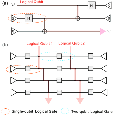
Quantum-gate circuits ${U_{C}}$ describe a sequence of quantum operations on a multi-qubit quantum state. In the circuit, the quantum information flows from the left end to the right end. Given an input state $\left|0\right\rangle$ and an output state $\left|i\right\rangle$ , the circuit is equivalent to a complex number $\left\langle i\right|{U_{C}}\left|0\right\rangle$ , called probability amplitudes. A key observation is that the circuit can also be interpreted as a quantum information network, where the lines guide the flow of information and the gate boxes represent local information operations. The lines include the world lines of physical qubits and the entangling lines of two-qubit gates. As all the lines merely represent quantum correlations, quantum information can flow along the lines at arbitrary direction. So, we can define new virtual logical qubits at some ports of the network and redirect the information flow along the lines while keeping the final probability amplitudes unchanged.

This concept is inspired from quantum teleportation protocol, as illustrated in Fig. 1(a). The original quantum teleportation circuit has three physical qubits. A new logical qubit can be defined and used to redirect the information flow along the circuit topological structure and implement the quantum information transfer.

We note that the number of virtual logical qubits can be smaller than the physical qubits. We can use this feature to renormalize a low-depth quantum circuit with large numbers of physical qubits to a new circuit with far less logical qubits. We show the basic idea in Fig. 1(b). A low-depth circuit consists of several layers of two-qubit entangling gates. Logical qubits are defined and flow transversely along these layers. The roles of world lines and entangling lines in the circuit network are exchanged, where logical qubits exist on the entangling lines and they are entangled by the world lines. Due to the number of logical qubits is proportional to the circuit’s depth, this method, transversal computation, implements a memory-efficient classical simulation for low-depth circuits.

The basic mathematical principle underlying the method is that a quantum-gate circuit is translated to a tensor network and then the tensor network is translated back to a new quantum-gate circuit. That is, two different quantum-gate circuits can share the same tensor network. Examples of transformation widgets are shown in the Supplementary Materials.

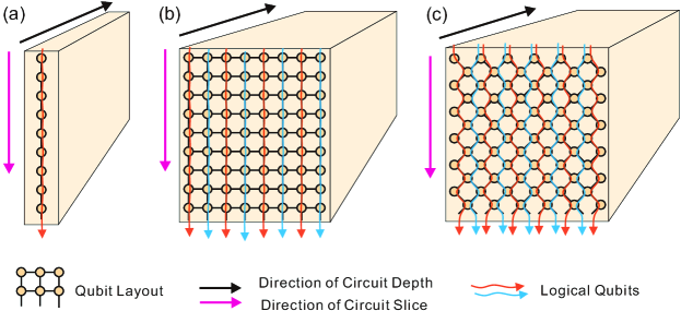
Next, we demonstrate how to use transversal computation to simulate several random quantum circuits. In the first example, the qubits are arranged on a 1D chain with nearest-neighbor interaction 1d ; 1d1d . The quantum-gate circuit consists of alternating layers of random single-qubit gates and two-qubit controlled-phase (CZ) gates, as shown in Fig. 1(b) and Fig. 2(a). Logical qubits are transversely defined along the layers of entangling gates: a CZ layer (a circuit depth) has a logical qubit. Therefore, an $N$ -qubit $L$ -depth circuit is mapped into a new $L$ -qubit $N$ -depth circuit. With 1 Petabyte memory, when the depth of the original circuit is smaller than 49 49q , the new circuit can be fully stored and directly simulated by the mature technology of sparse matrix-vector multiplication.

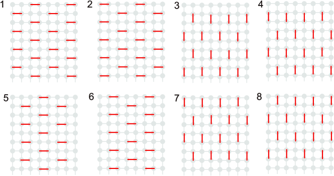
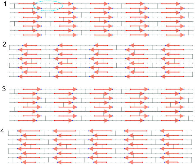
The second example is to simulate quantum-gate circuits of 2D-grid qubits, which are proposed for quantum computational supremacy experiment with superconducting quantum circuits complex2D . The qubits are arranged on the vertices of an $M\times N$ ( $M\geq N$ ) grid. The quantum circuit consists of repetitive patterns of CZ gates, where every $8$ depths of the circuit can make each pair of the nearest-neighbor qubits entangle by a single CZ gate. Meanwhile, random single-qubit gates are placed on some idle qubits in each depth. We define $N$ logical qubits (equal to the column number $N$ ) for every $8$ circuit depths, and we transversely divided the circuit into $M$ slices (equal to the row number $M$ ), as shown in Fig. 2(b). The logical qubits go forward or backward on the world lines inside the slices and go across adjacent slices by the entangling lines, in the same style of the quantum teleportation circuit in Fig. 1(a). We show the details of each slice in the Supplementary Materials. Therefore, for $M\times N$ -qubit $8\times L$ -depth circuits, the number of logical qubits is $N\times L$ , which is smaller than the number of physical qubits when $M>L$ .

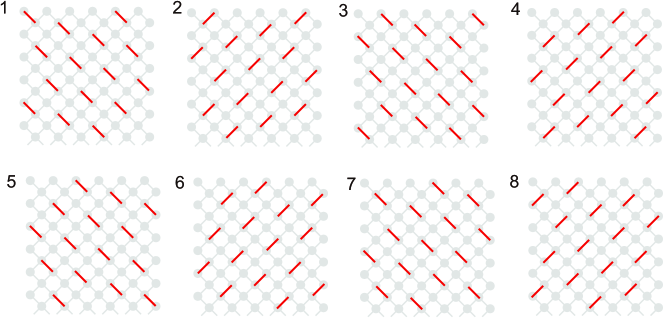
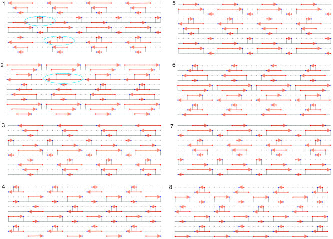
The third example is a modified version of the above 2D layout of qubits. In the new 2D-Bristlecone layout, the qubit grid is rotated by ${45^{\circ}}$ with a diamond boundary and the repetitive patterns of CZ gates are reordered simu0.005 . For an $M\times N$ ( $M\geq N$ ) grid, we define $2N-1$ logical qubits for every $8$ circuit depths. The flow of the logical qubits is shown in Fig. 2(c) and the details of transversal circuit slices are shown in the Supplementary Materials. So, for $M\times N$ -qubit $8\times L$ -depth circuits, the number of logical qubits is $(2N-1)\times L$ .

We simulate three circuit examples on the supercomputer Sunway TaihuLight sunway . The Sunway has $40960$ computing nodes and each node has $32$ Gigabytes memory and $3$ TFLOPS performance. The total memory is $1.25$ Petabytes, so a state vector of up to $48$ logical qubits can be stored. Here, we choose to simulate 1D-chain $1000$ -qubit $42$ -depth, 2D-grid $125\times 8$ -qubit $42$ -depth and 2D-Bristlecone $12\times 6$ -qubit $32$ -depth circuits by applying $42$ , $40$ and $44$ logical qubits, respectively. As ordinary optimization methods for quantum gate circuit simulation can be directly adopted, we design a simulator based on the evolution of wave-function according to the optimizations in simuLi . The simulator uses 4096, 1024, 16384 computing nodes to produce a probability amplitude in $297.8$ , $131.6$ and $14.1$ minutes, respectively.

After the circuit simulations, we need a subsequent step to generate samples from the calculated probability amplitudes for the task of quantum circuit sampling. In general, it will consume several probability amplitudes to produce a sample. For example, Metropolis sampling using about $100$ probability amplitudes mcmc and frugal rejection sampling simuNew using a batch of tens probability amplitudes are proposed to produce one effective sample. Here, we show that a simple threshold-rejection sampling method has a sweet spot between the sampling efficiency and the sample fidelity.

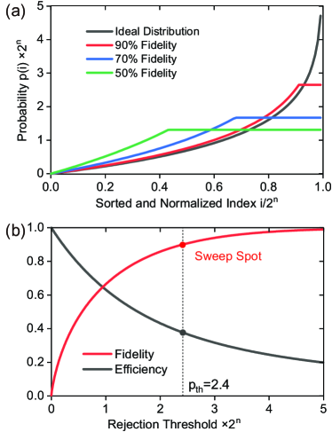
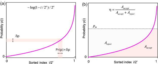
The population $\left\{{p(i)|i=0,...,{2^{n}}-1}\right\}$ of an $n$ -qubit random quantum state obeys an exponential distribution complex2D . When sorting the population in ascending order, it has function shape $p(i)=-\ln(1-i/{2^{n}})/{2^{n}}$ , which has a high-and-narrow peak and a long tail. We carefully choose a threshold ${p_{th}}$ to cut the distribution and get a new renormalized distribution with a flat top to approximate the ideal distribution, as shown in Fig. 3(a). Then, we use native rejection sampling to produce samples according to this new flat-top distribution by repeating the following steps: (1) suggesting a random sample $i$ and calculate its probability $p(i)$ ; (2) accepting the sample with a probability of $\min\left({p(i)/{p_{th}},1}\right)$ .

We show the trade-off between sampling efficiency and sample fidelity in Fig. 3(b). When setting the threshold to $2.4\times{2^{-n}}$ , we get the sample fidelity of $0.9$ with sampling efficiency of $0.38$ . That is, this threshold-rejection sampler can produce one statistically-independent and high-fidelity sample by consuming about $3$ probability amplitudes.

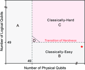
Our results significantly extend both the scale and efficiency of classical simulation of random quantum sampling. We show the phase transition of classical hardness of random quantum circuits in Fig. 4. We identify an enlarged classically-easy area, where a new 49-qubit memory barrier emerges. For a quantum circuit with less than 49 logical qubits, the running time of transversal computation is proportional to the number of physical qubits, while the number of logical qubits is proportional to the circuit depth. We note that hybrid algorithms by mixing Schrodinger and Feynman methods complexQubit can be further used to exploit the trade-off between memory usage and running time to slightly extend the classically-easy area.

In summary, we have described a quantum teleportation-inspired algorithm to simulate low-depth random quantum circuits of a large number of qubits. The algorithm is memory-efficient and has a physically intuitive picture. Our work not only adds a new tool to efficiently simulate quantum circuits but also extend the versatile concept of quantum teleportation to enhance classical technology.

References

(1) Nielsen, M. A. & Chuang, I. L. Quantum Computation and Quantum Information: 10th Anniversary Edition (Cambridge University Press, New York, NY, USA, 2011), 10th edn.
(2) Harrow, A. W., Hassidim, A. & Lloyd, S. Quantum algorithm for linear systems of equations. Physical review letters 103, 150502 (2009).
(3) Aspuru-Guzik, A., Dutoi, A. D., Love, P. J. & Head-Gordon, M. Simulated quantum computation of molecular energies. Science 309, 1704–1707 (2005).
(4) Barends, R. et al. Superconducting quantum circuits at the surface code threshold for fault tolerance. Nature 508, 500 (2014).
(5) Ballance, C. J., Harty, T. P., Linke, N. M., Sepiol, M. A. & Lucas, D. M. High-fidelity quantum logic gates using trapped-ion hyperfine qubits. Phys. Rev. Lett. 117, 060504 (2016).
(6) Gaebler, J. P. et al. High-fidelity universal gate set for ${{}^{9}\mathrm{Be}}^{+}$ ion qubits. Phys. Rev. Lett. 117, 060505 (2016).
(7) Aaronson, S. & Arkhipov, A. The computational complexity of linear optics. In Proceedings of the forty-third annual ACM symposium on Theory of computing, 333–342 (ACM, 2011).
(8) Aaronson, S. & Chen, L. Complexity-theoretic foundations of quantum supremacy experiments. arXiv preprint arXiv:1612.05903 (2016).
(9) Harrow, A. W. & Montanaro, A. Quantum computational supremacy. Nature 549, 203 (2017).
(10) Bouland, A., Fefferman, B., Nirkhe, C. & Vazirani, U. On the complexity and verification of quantum random circuit sampling. Nature Physics 1 (2018).
(11) Preskill, J. Quantum computing in the nisq era and beyond. arXiv preprint arXiv:1801.00862 (2018).
(12) Boixo, S. et al. Characterizing quantum supremacy in near-term devices. Nature Physics 14, 595 (2018).
(13) Neill, C. et al. A blueprint for demonstrating quantum supremacy with superconducting qubits. Science 360, 195–199 (2018).
(14) Dalzell, A. M., Harrow, A. W., Koh, D. E. & La Placa, R. L. How many qubits are needed for quantum computational supremacy? arXiv preprint arXiv:1805.05224 (2018).
(15) Biamonte, J. D., Morales, M. E. & Koh, D. E. Quantum supremacy lower bounds by entanglement scaling. arXiv preprint arXiv:1808.00460 (2018).
(16) Pednault, E. et al. Breaking the 49-qubit barrier in the simulation of quantum circuits. arXiv preprint arXiv:1710.05867 (2017).
(17) Markov, I. L. & Shi, Y. Simulating quantum computation by contracting tensor networks. SIAM Journal on Computing 38, 963–981 (2008).
(18) Boixo, S., Isakov, S. V., Smelyanskiy, V. N. & Neven, H. Simulation of low-depth quantum circuits as complex undirected graphical models. arXiv preprint arXiv:1712.05384 (2017).
(19) Chen, Z.-Y. et al. 64-qubit quantum circuit simulation. Science Bulletin (2018).
(20) Li, R., Wu, B., Ying, M., Sun, X. & Yang, G. Quantum supremacy circuit simulation on sunway taihulight. arXiv preprint arXiv:1804.04797 (2018).
(21) Chen, J., Zhang, F., Huang, C., Newman, M. & Shi, Y. Classical simulation of intermediate-size quantum circuits. arXiv preprint arXiv:1805.01450 (2018).
(22) Markov, I. L., Fatima, A., Isakov, S. V. & Boixo, S. Quantum supremacy is both closer and farther than it appears. arXiv preprint arXiv:1807.10749 (2018).
(23) Villalonga, B. et al. A flexible high-performance simulator for the verification and benchmarking of quantum circuits implemented on real hardware. arXiv preprint arXiv:1811.09599 (2018).
(24) Bennett, C. H. et al. Teleporting an unknown quantum state via dual classical and einstein-podolsky-rosen channels. Physical review letters 70, 1895 (1993).
(25) Raussendorf, R. & Briegel, H. J. A one-way quantum computer. Physical Review Letters 86, 5188 (2001).
(26) Emerson, J., Weinstein, Y. S., Saraceno, M., Lloyd, S. & Cory, D. G. Pseudo-random unitary operators for quantum information processing. science 302, 2098–2100 (2003).
(27) Weinstein, Y. S., Brown, W. G. & Viola, L. Parameters of pseudorandom quantum circuits. Physical Review A 78, 052332 (2008).
(28) De Raedt, H. et al. Massively parallel quantum computer simulator, eleven years later. arXiv preprint arXiv:1805.04708 (2018).
(29) Fu, H. et al. The sunway taihulight supercomputer: system and applications. Science China Information Sciences 59, 072001 (2016).
(30) Neville, A. et al. Classical boson sampling algorithms with superior performance to near-term experiments. Nature Physics 13, 1153 (2017).

Supplementary Information

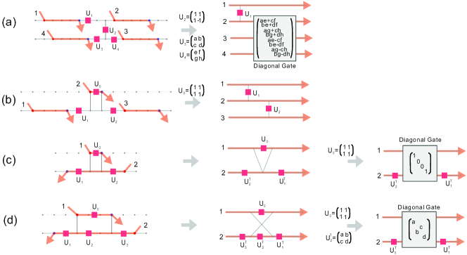
Logical gates for logical qubits. There are two steps in transversal computation to produce a new circuit. (1) Define logical qubits along the circuit topology; (2) Translate the residual circuits between logical qubits back to logical gates. In Fig. S1, we show several basic circuit transformation widgets for the 1D circuits. For the 2D-grid (see Fig. S2) and 2D-Bristlecone (see Fig. S3) circuits, we show the details of the logical qubits in each circuit slice in Fig. S4 and Fig. S5, respectively. In Fig. S6, we show representative circuit widgets to fabricate logical gates in these new circuits.

Sampling efficiency and sample fidelity. The population $\{p(i)|i=0,...,{2^{n}}-1\}$ of a n-qubit random quantum state obeys an exponential distribution $\Pr(p)={e^{-2^{n}\times p}}$ . When sorting the population in ascending order, the function shape is $p(i)=-\log(1-i/{2^{n}})/{2^{n}}$ , as shown in Fig. S7(a). We use a threshold ${p_{th}}$ to cut the ideal (sorted) distribution $p(i)$ , and obtain an approximate distribution $\tilde{p}(i)=\left\{{\begin{array}[]{*{20}{c}}{\frac{{-\log(1-i/{2^{n}})/{2^{n}}}}{{1-{e^{-{p_{th}}}}}},}&{0\leq i<{2^{n}}(1-{e^{-{p_{th}}}})}\\ {\frac{{{p_{th}}}}{{1-{e^{-{p_{th}}}}}},}&{{2^{n}}(1-{e^{-{p_{th}}}})\leq i<{2^{n}}}\end{array}}\right.$ . Threshold-rejection sampling method is used to generate samples. The random suggested samples are accepted with a ratio ${A_{accept}}$ and rejected with a ratio ${A_{reject}}$ , as shown in Fig. S7(b). So, the sampling efficiency is $\eta=\frac{{{A_{accept}}}}{{{A_{accept}}+{A_{reject}}}}=\frac{{\sum\nolimits_{i=0}^{{2^{n}}-1}{\min(p(i),{p_{th}})}}}{{{2^{n}}{p_{th}}}}$ . The fidelity of the samples from noisy quantum state $\rho\approx f\left|\psi\right\rangle\left\langle\psi\right|+(1-f)\frac{I}{{{2^{n}}}}$ is measured by cross-entropy fidelity ${f_{CE}}$ , which is equal to the quantum state fidelity $f$ . The cross-entropy fidelity is ${f_{CE}}\approx\left({\log{2^{n}}+0.577}\right)-\sum\nolimits_{i=0}^{{2^{n}}-1}{\tilde{p}(i)\times\log\frac{1}{{p(i)}}}$ . We use cross-entropy fidelity to characterize the effective samples generated by a threshold-rejection sampler.