Model-free measurement of the pair potential in colloidal fluids using optical microscopy

Abstract

We report a straightforward, model-free approach for measuring pair potentials from particle-coordinate data, based on enforcing consistency between the pair distribution function measured separately by the distance-histogram and test-particle insertion routes. We demonstrate the method’s accuracy and versatility in simulations of simple fluids, before applying it to an experimental system composed of superparamagnetic colloidal particles. The method will enable experimental investigations into many-body interactions and allow for effective coarse-graining of interactions from simulations.

The versatility of colloidal particles as model systems for condensed matter physics can hardly be overstated, as illustrated through studies in crystallisation Tan et al. (2014); Feng et al. (2015), glasses Schall et al. (2007); Mattsson et al. (2009), gels Lu et al. (2008), interfacial phenomena Aarts et al. (2004), and rheology Cheng et al. (2011). Moreover, the colloidal interactions can be engineered to give rise to novel self-assembled phases Sacanna et al. (2010); Chen et al. (2011) with exciting potential applications. Despite these tremendous successes for colloid science, quantitative comparisons between experiments and theory or simulations, and thus more accurate and powerful predictions from those theoretical tools, hinge on precise knowledge of the interparticle interactions. These interactions are often only approximately known and are based on theoretical assumptions, for example that the particles interact through a DLVO or depletion potential Israelachvili (2015).

Existing methods to measure the pair potential come with certain drawbacks: methods based on inverting correlation functions rely on additional assumptions Carbajal-Tinoco et al. (1996); Rajagopalan and Srinivasa Rao (1997); Behrens and Grier (2001); Quesada-Pérez et al. (2001) or large numbers of computer simulations Schommers (1973); Levesque et al. (1985); Brunner et al. (2002); Royall et al. (2003), and direct methods Crocker and Grier (1994); Piech and Walz (2002); Hertlein et al. (2008) are typically carried out away from the equilibrium context, measured only between two particles or a particle and a wall. Furthermore, these methods can be technically demanding, both in the lab and numerically, and are therefore not routinely employed. By contrast, in this report we provide a versatile, fast, model-free approach which allows an effective pair potential to be determined solely from particle coordinates obtained using optical microscopy, based on a novel inversion of the pair distribution function. The method is broadly applicable in fields dealing with the liquid state, ranging from soft matter to biophysics, as well as in a wide range of industries where colloidal systems are used.

The pair distribution function $g$ offers a real-space visualisation of pairwise structure. It provides a direct link to the phase behaviour and thermodynamic properties of the system if the interparticle interactions are known Hansen and McDonald (2013). For a homogeneous fluid, $g$ is given by the ratio of the local number density about a reference particle, $\rho^{(0)}(\mathbf{r})$, and the bulk number density, $\rho$:

$$g(\mathbf{r})=\frac{\rho^{(0)}(\mathbf{r})}{\rho}\mathrm{,}$$ (1)

where $\mathbf{r}$ is the position vector relative to the reference particle. In experiments and simulations, $\rho^{(0)}(\mathbf{r})$ is typically measured using a distance-histogram method Allen and Tildesley (2017).

Here, we propose an alternative approach based on test-particle insertion Henderson (1983); Stones et al. (2018); Widom (1963), with $g$ again given by a ratio of local and bulk ensemble averages:

$$g(\mathbf{r})=\frac{\langle\exp(-\Psi/k_{\mathrm{B}}T)\rangle^{(0)}_{\mathbf{r}}}{\langle\exp(-\Psi/k_{\mathrm{B}}T)\rangle}\mathrm{,}$$ (2)

in which $\Psi$ is the additional potential energy due to the hypothetical insertion of a particle and $k_{\mathrm{B}}T$ is the thermal energy. The potential energy $\Psi$ is written as a sum of pairwise interactions, depending on the effective pair potential $u$ between the particles in the fluid. For a homogeneous system at a given density, $u$ giving rise to a particular $g$ is unique Henderson (1974). Crucially, matching $g$ from insertion with that from the distance-histogram method provides an elegant route to obtain the pair potential $u$.

We will first explain the method, before demonstrating its use and accuracy in simulation. We then apply the method to a colloidal model system composed of superparamagnetic particles, in which the pairwise interaction can be tuned using an external magnetic field Promislow et al. (1995). The experimental demonstration is for a quasi-two dimensional one-component fluid composed of particles with isotropic interactions, but we stress that equation (2) holds for anisotropic interactions in any dimension and may be extended to multi-component fluids.

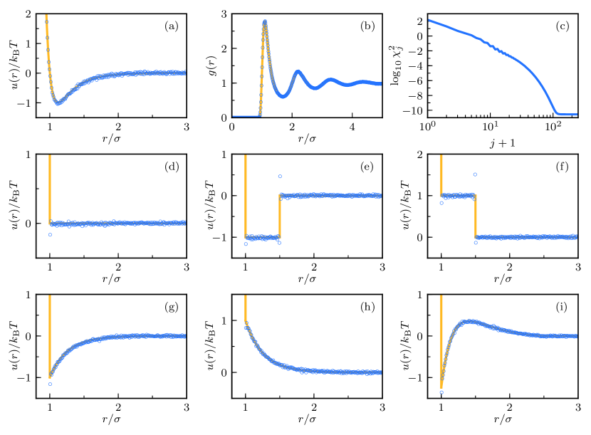
Figure 1: (a) Lennard-Jones $u(r)$ measured using the method presented here (blue circles), compared with the simulation input (yellow line). (b) Corresponding $g(r)$ obtained by the distance-histogram method (yellow line) and by test-particle insertion with the measured pair potential (blue circles). (c) Log-log plot showing convergence of the PC scheme. Remaining panels show pair potentials measured for (d) a hard-disk potential, (e) a hard-core attractive square-well potential, (f) a hard-core repulsive square-well potential, (g) an attractive Yukawa potential, (h) a repulsive Yukawa potential, (i) a hard-core two-Yukawa (HCTY) potential.

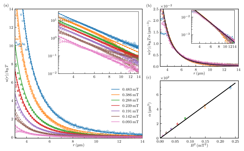
Figure 2: (a) Repulsive dipolar pair potentials measured for two samples at different number densities (Sample 1—triangles and dashed lines, Sample 2—circles and solid lines) in experiment for different $B$; the lines are fits to (5). Inset: corresponding log-log plot where the pair potentials appear as parallel straight lines with slope $-3$. (b) When divided by the fitting parameter $\alpha$, the measured pair potentials collapse onto a single curve. (c) Plot of $\alpha$ against $B^{2}$—as anticipated, the data fall on a straight line.

To find $u$, a predictor-corrector (PC) scheme proposed by Schommers Schommers (1973) is used. Briefly, a trial pair potential $u_{j}(r)$—here, we begin with $u_{0}(r)=0$ everywhere—is used in equation (2) to obtain a prediction of the pair distribution function $g_{j}(r)$. This is compared with the distance-histogram result $g_{\mathrm{h}}(r)$ using

$$u_{j+1}(r)=u_{j}(r)-k_{\mathrm{B}}T\ln\left(\frac{g_{\mathrm{h}}(r)}{g_{j}(r)}\right)\mathrm{,}$$ (3)

to obtain a corrected pair potential $u_{j+1}(r)$. This scheme is performed iteratively until convergence, which is verified by monitoring the value of

$$\chi_{j}^{2}=\sum_{k=0}^{k=N}(g_{j}(r_{k})-g_{\mathrm{h}}(r_{k}))^{2}\mathrm{,}$$ (4)

where the $r_{k}$ are the mid-points of the bins used in the distance-histogram method. In contrast with inverse Monte Carlo schemes Schommers (1973); Levesque et al. (1985), the calculation of $g_{j}(r)$ required for the corrector step (3) is performed using test-particle insertion on the existing particle coordinates and each iteration does not require an additional (expensive) simulation. The distances between each test-particle and those of the fluid need to be calculated only once, allowing for a very efficient implementation. A more detailed account of the implementation of this PC scheme is provided in the supplemental material sup .

The scheme was first tested using particle coordinates generated by Monte Carlo simulations, where the measured pair potentials can be compared to the simulation input sup . Figure 1(a-c) demonstrates the use of the method with data from a two-dimensional Lennard-Jones simulation. The agreement between the measured and input pair potentials is excellent. As expected, the PC scheme enforces consistency between the two methods, converging after $\sim\!100$ iterations (see Figure 1(c))—in the other cases, the convergence is even faster.

Figures 1(d-i) show the application of the method to a wide range of pair potentials of interest in liquid-state theory and colloid science, including hard disks Thorneywork et al. (2017), attractive and repulsive square-well potentials, attractive and repulsive hard-core Yukawa potentials, and a hard-core two-Yukawa potential Rudisill and Cummings (1989) with competing short-range attractions and long-range repulsions—in all cases the input pair potential is recovered. We particularly note the discontinuities in the input pair potentials, which are captured by our analysis.

Next, we apply the method to an experimental colloidal model system, where the pair potential is generally unknown, illustrating the strength of our method. We used a quasi two-dimensional system of superparamagnetic colloidal particles with a diameter $\sigma\approx$3\text{\,}\mathrm{\SIUnitSymbolMicro m}$$, which acquire a magnetic dipole moment when placed in an external magnetic field sup . Outside of the core region ($r>\sigma$), the particles are expected to interact with a repulsive dipolar pair potential

$$\frac{u(r)}{k_{\mathrm{B}}T}=\frac{\alpha}{r^{3}}\mathrm{,}$$ (5)

with $\alpha$ proportional to the square of the magnetic flux density $B$ Promislow et al. (1995). This system is particularly useful for this investigation since several different $u(r)$ can be measured using a single sample by altering $B$.

The measured pair potentials are shown in Figure 2(a) for two different particle number densities—in all cases, a pair potential is readily extracted showing the expected inverse-cube decay, as illustrated on the log-log plot of the inset. Equation (5) can be used to extract a value of $\alpha$ for each $u(r)$, with larger $B$ inducing a larger dipole moment in each particle, corresponding to a stronger dipolar repulsion. The measured pair potentials collapse onto a single curve after dividing by the values of $\alpha$ found from the fit, as shown in Figure 2(b). In Figure 2(c), the extracted values of $\alpha$ are plotted against $B^{2}$, yielding the anticipated straight line. Finally, we note that for a given $B$, the same pair potential is obtained in both samples, showing that at these densities the system is pairwise additive.

In summary, we have demonstrated a novel method for measuring pair potentials in colloidal systems. The method is readily extended to three-dimensional and multi-component systems, and will be a valuable tool in characterising colloidal particles used in fundamental and applied studies. The experimental and computational requirements are minimal: a simple transmission light microscope to obtain the particle snapshots and a desktop computer will suffice. Standard image analysis routines may be used to obtain the particle coordinates and the computational scheme can be straightforwardly encoded and run. We stress that no assumptions about the form of the pair potential have to be made. In addition to clear industrial applications, where knowledge of interparticle interactions is often essential in formulation of products, the method will allow for fundamental investigations into many-body interactions, such as those arising in the controversy around like-charge attractions Grier (1998), and enables coarse-grained pair potentials Lyubartsev and Laaksonen (1995) to be derived for use in multi-scale simulations of more complex fluids and biological systems.