The fully-visible Boltzmann machine and the Senate of the 45th Australian Parliament in 2016

Abstract

After the 2016 double dissolution election, the 45th Australian Parliament was formed. At the time of its swearing in, the Senate of the 45th Australian Parliament consisted of nine political parties, the largest number in the history of the Australian Parliament. Due to the breadth of the political spectrum that the Senate represented, the situation presented an interesting opportunity for the study of political interactions in the Australian context. Using publicly available Senate voting data in 2016, we quantitatively analyzed two aspects of the Senate. Firstly, we analyzed the degree to which each of the non-government parties of the Senate are pro- or anti-government. Secondly, we analyzed the degree to which the votes of each of the non-government Senate parties are in concordance or discordance with one another. We utilized the fully-visible Boltzmann machine (FVBM) model in order to conduct these analyses. The FVBM is an artificial neural network that can be viewed as a multivariate generalization of the Bernoulli distribution. Via a maximum pseudolikelihood estimation approach, we conducted parameter estimation and constructed hypotheses test that revealed the interaction structures within the Australian Senate. The conclusions that we drew are well-supported by external sources of information.

^∗Corresponding author email: j.bagnall@latrobe.edu.au. ¹Department of Mathematics and Statistics, La Trobe University, Bundoora Melbourne, 3086 Australia. ²School of Mathematics and Physics, University of Queensland, St. Lucia Brisbane, 4072 Australia.

Key words: Australian Parliament, Bernoulli distribution, maximum pseudolikelihood estimation, minorization-maximization algorithm, neural networks, parametric model

1 Introduction

At the federal level, or Commonwealth level, the Australian parliamentary government system is composed of two houses, the House of Representatives, and the Senate (cf. Weller and Fleming, 2003). The House of Representatives is composed of members who represent, and are elected by a nearly equal numbers of voters (currently approximately 150,000 individuals) from the public. We make a note that the electorates of Tasmania are notably smaller than the other states (currently approximately 100,000 individuals).

Furthermore, members of the House of Representatives are tasked with the role of debating legislation and government policy, raising matters of concern, and importantly making laws via the introduction of bills, or in the language of the Constitution, proposed laws. Currently, the House of Representatives consists of 150 members of parliament. We refer the interested reader to Wright and Fowler (2012) regarding information about the House of Representatives of Australia.

In contrast to the House of Representatives, the Senate consists of 76 senators, who do not equally represent the population, but the states and territories, instead. That is, each of the six states (i.e. New South Wales, Queensland, South Australia, Tasmania, Victoria, and Western Australia) are equally represented by 12 senators, and each of the two territories (i.e the Australian Capital Territory, and the Northern Territory) are represented by two senators (cf. Evans, 2016, Ch. 1).

For any bill to pass to law, both the House of Representatives and the Senate must assent to the bill, requiring a simple majority vote in each house. As such, the primary function of the senate is to represent the people of each of the states and territories equally. It acts as a balance of power between the states with large populations and the states with smaller populations, who are not able to secure numbers in the House of Representatives. Although the Senate does not have the complete suite of powers to introduce bills, when compared to the House of Representatives (e.g. the Senate cannot introduce taxing bills, appropriation bills, or amend such bills), the Senate does have the power to reject any bills that are introduced by the House of Representative, and request the amendment of introduced bills. More information regarding the Australian Senate and its powers can be found in Evans (2016).

In 2016, following a double dissolution election (cf. Gauja et al. (2018); Corcoran and Dickenson, 2010 define a double dissolution election as one where all seats of the House of Representatives and the Senate are simultaneously contested), the Senate of the 45th Australian Parliament was formed. In normal election cycles of three years, only half of the senators from each state face reelection, since each senator is elected to a six year term (cf. Evans, 2016, Ch. 1). The territorial senators are elected to three year terms at all elections, and thus face no special consequence from the special election. The double dissolution is therefore particularly interesting, as the elected state senators all face reelection simultaneously, and thus the composition of the seated Senate is more volatile than after a normal election. The elected Senate consisted of senators from nine separate political parties, which is the largest number of political parties in the history of the Senate (cf. Evans, 2016, Tab. 2). At the time of its swearing in, the Senate of the 45th Australian Parliament consisted of 30 senators from the governing Liberal National Party (LNP), 26 senators from the opposition Australian Labour Party (ALP), 9 senators from the Australian Greens (AG), 4 senators from Pauline Hanson’s One Nation (PHON), 3 senators from the Nick Xenophon Team (NXT), 1 Liberal Democratic Party (LDP) senator, 1 Family First Party (FFP) senator, 1 Jacqui Lambie Network (JLN) senator, and 1 Derryn Hinch Justice Party (DHJP) senator.

When Senators vote on an item of legislation or a motion, the event is known as a division (cf. Corcoran and Dickenson, 2010). Divisions data, at a party level, are recorded on the official Australian Parliament website at the URL: www.aph.gov.au/Parliamentary_Business/Statistics/Senate_StatsNet/General/divisions.

In this article, we analyze the data from the first sitting of the Senate of the 45th Australian Parliament, until the final sitting of the year 2016. The first division during this period was conducted on the 31st of August 2016, and the last division was performed on the 1st of December 2016. In total, 147 divisions were performed during this period. We have chosen this period due to the particular stability of the Senate during the time. After this period, a number of events, including the so-called dual citizenship crisis (see, e.g. Begg, 2017 and Hobbs et al., 2018) resulted in a high number of turnover and changes in the Senate composition.

We seek to quantitatively analyze two aspects of the Senate. Firstly, we analyze the degree to which each of the non-government parties of the Senate are pro- or anti-government. Secondly, we analyze the degree to which the votes of each of the non-government Senate parties are in concordance or discordance with one another. In order to answer both questions we seek to analyze the division data using a fully-visible Boltzmann machine (FVBM).

The Boltzmann machine (BM) is a parametric generative graphical probabilistic artificial neural network (ANN) that was introduced in the seminal paper of Ackley et al. (1985). The BM is a deep ANN with a latent variable structure that is capable of universal representation of the probability mass function (PMF) of multivariate binary random variables of any fixed dimension $d\in\mathbb{N}$ (cf, Le Roux and Bengio, 2008).

The FVBM, introduced in Hyvarinen (2006), is a simplification of the BM, which does not contain a hidden variable structure. It is a type of log-linear graphical generative probabilistic model that is comparable to the models that are studied in Lauritzen (1996). It can also be considered as a multivariate generalization of the Bernoulli random variable and is equivalent to the logistic multivariate binary model proposed by Cox (1972). Our use of the FVBM is motivated by that of Desmarais and Crammer (2010) who construct FVBMs for the analysis of relationships between judges in the United States Supreme Court, using data from 178 cases in the period between 2007 and 2008.

In Hyvarinen (2006), it was proved that an unknown parameter vector that determines the data generating process (DGP) of data arising from an FVBM can be estimated consistently via maximum pseudolikelihood estimation (MPLE) (also known as maximum composite likelihood estimation; see Lindsay, 1988 and Arnold and Strauss, 1991). An alternative proof of consistency can be found in Nguyen (2018).

Following from the work of Hyvarinen (2006), Nguyen and Wood (2016a) proved that the consistent maximum pseudolikelihood estimator (MPLE) of an FVBM is also asymptotically normal. Furthermore, in Nguyen and Wood (2016b), it was demonstrated that the MPLE for an FVBM could be efficiently computed from data via an iterative block-successive lower bound maximization algorithm of the kind that is described in Razaviyayn et al. (2013). It was proved that the computational algorithm monotonically increases the pseudolikelihood objective in each iteration, and that the limit point of the algorithm is a global maximum of the objective function. In this paper, we utilize the R package BoltzMM (Jones and Nguyen, 2018), which implements the methods and algorithms that are described in Nguyen and Wood (2016a) and Nguyen and Wood (2016b), for the analysis of the our Senate data.

The remainder of the article proceeds as follows. In Section 2, we describe the FVBM, the MPLE estimator, and the inferential tools that we will use. In Section 3, we describe our Senate data in detail, and we discuss the details of our data processing protocol. In Section 4, we present the result of an analysis of the Senate data via an FVBM and we discuss the results of the analysis. In Section 5, we draw some conclusions regarding our work. Auxiliary and technical results are presented in the Appendix.

2 The fully-visible Boltzmann machine

Let $\bm{X}^{\top}=\left(X_{1},\dots,X_{d}\right)$ be a vector of spin binary random variables (i.e. $X_{j}\in\left\{-1,+1\right\}$; $j\in\left[d\right]=\left\{1,\dots,d\right\}$). Here, $\left(\cdot\right)^{\top}$ is the transposition operator. We say that the DGP of $\bm{X}$ is a FVBM if it can be characterized by the PMF

$$f\left(\bm{x};\bm{\theta}\right) =\mathbb{P}\left(\bm{X}=\bm{x}\right)$$

$$=\frac{\exp\left(\frac{1}{2}\bm{x}^{\top}\bm{M}\bm{x}+\bm{x}^{\top}\bm{b}\right)}{z\left(\bm{\theta}\right)}\text{,}$$ (1)

where

$$z\left(\bm{\theta}\right)=\sum_{\bm{\xi}\in\left\{-1,1\right\}^{d}}\exp\left(\frac{1}{2}\bm{\xi}^{\top}\bm{M}\bm{\xi}+\bm{\xi}^{\top}\bm{b}\right)\text{,}$$

$\bm{M}\in\mathbb{R}^{d\times d}$ is a symmetric matrix with zeros along the diagonal, and $\bm{b}\in\mathbb{R}^{d}$. We call $z\left(\bm{\theta}\right)$ the normalization constant, and we put the unique elements of $\bm{M}$ and $\bm{b}$ into the $\left[n\left(n-1\right)/2+n\right]$-dimensional parameter vector $\bm{\theta}$.

The bias vector $\bm{b}$ can be written as:

$$\bm{b}^{\top}=\left(b_{1},\dots,b_{d}\right)\text{,}$$

where increasing the value of $b_{j}\in\mathbb{R}$ ($j\in\left[d\right]$) increases the probability $\mathbb{P}\left(X_{j}=+1\right)$, ceteris paribus. Similarly, decreasing the value of $b_{j}$ increases the probability $\mathbb{P}\left(X_{j}=-1\right)$, ceteris paribus.

The interaction matrix $\bm{M}$ can be written as:

$$\bm{M}=\left[\begin{array}[]{ccccc}0&m_{12}&m_{13}&\dots&m_{1d}\\ m_{12}&0&m_{23}&\dots&m_{2d}\\ m_{13}&m_{23}&0&\ddots&\vdots\\ \vdots&\vdots&\ddots&\ddots&m_{d-1,d}\\ m_{1d}&m_{2d}&\cdots&m_{d-1,d}&0\end{array}\right]\text{,}$$

where increasing the value of $m_{jk}\in\mathbb{R}$ ($j,k\in\left[d\right]$; $j<k$) increases the probability $\mathbb{P}\left(X_{j}=X_{k}\right)$, ceteris paribus. Similarly, decreases in the value of $m_{jk}$ increases the probability $\mathbb{P}\left(X_{j}\neq X_{k}\right)$, ceteris paribus. Thus, the vector $\bm{b}$ controls the marginal probabilities of each element of $\bm{X}$, whereas the matrix $\bm{M}$ controls the correlations between the elements of $\bm{X}$.

2.1 Estimation of the FVBM parameter vector

Suppose that we observe $n$ independent and identical replicates of $\bm{X}$, say $\bm{X}_{1},\dots,\bm{X}_{n}$, which arise from a DGP that can be characterized by an FVBM with unknown parameter vector $\bm{\theta}_{0}$. Since the FVBM is a probabilistic model with PMF (1), we can construct the log-likelihood function

$$l_{n}\left(\bm{\theta}\right) =\sum_{i=1}^{n}\log f\left(\bm{X}_{i};\bm{\theta}\right)$$

$$=\frac{1}{2}\sum_{i=1}^{n}\bm{X}_{i}^{\top}\bm{M}\bm{X}_{i}+\sum_{i=1}^{n}\bm{X}_{i}^{\top}\bm{b}-n\log z\left(\bm{\theta}\right)\text{,}$$

and estimate $\bm{\theta}_{0}$ via the maximum likelihood estimator (MLE)

$$\hat{\bm{\theta}}_{n}=\arg\max_{\bm{\theta}}\text{ }l_{n}\left(\bm{\theta}\right)\text{.}$$

Unfortunately, for all but the smallest values of $d$, the log-likelihood function is prohibitively computationally expensive to work with, since the number of terms in $z\left(\bm{\theta}\right)$ grows exponentially with $d$. Due to the computational costs of obtaining the MLE, it is more common to consider the MPLE as an estimator of $\bm{\theta}_{0}$ in the FVBM context, instead (see, e.g. Hyvarinen, 2006, Desmarais and Crammer, 2010, Nguyen and Wood, 2016b, and Nguyen and Wood, 2016a).

The so-called log-pseudolikelihood function, as used by the references above, can be written as

$$p_{n}\left(\bm{\theta}\right)=\sum_{i=1}^{n}\sum_{j=1}^{d}\log f\left(X_{ij}|\bm{X}_{i\left(j\right)};\bm{\theta}\right)\text{,}$$ (2)

where $\bm{X}_{\left(j\right)}^{\top}=\left(X_{1},\dots,X_{j-1},X_{j+1},\dots,X_{d}\right)$ and

$$f\left(x_{j}|\bm{x}_{\left(j\right)};\bm{\theta}\right)=\frac{\exp\left(x_{j}\bm{m}_{j}^{\top}\bm{x}+b_{j}x_{j}\right)}{\exp\left(\bm{m}_{j}^{\top}\bm{x}+b_{j}\right)+\exp\left(-\bm{m}_{j}^{\top}\bm{x}-b_{j}\right)}\text{.}$$

Here, $\bm{m}_{j}$ is the $j\text{th}$ column of $\bm{M}$, and we call $\prod_{j=1}^{d}f\left(X_{j}|\bm{X}_{\left(j\right)};\bm{\theta}\right)$ the individual pseudolikelihood of observation $\bm{X}$. Note that (2) no longer depends on the normalization constant $z\left(\bm{\theta}\right)$. Like the MLE, the MPLE can be defined as the maximizer of (2). That is, we can write the MPLE as

$$\tilde{\bm{\theta}}_{n}=\arg\max_{\bm{\theta}}\text{ }p_{n}\left(\bm{\theta}\right)\text{.}$$ (3)

2.2 Properties of the MPLE

The MPLE has a number of desirable asymptotic properties. Firstly, via the results of Hyvarinen (2006) and Nguyen (2018), the MPLE is proved to be a consistent estimator of $\bm{\theta}_{0}$ in the case when the FVBM is a well-specified model for the DGP of the data, and is proved to be Wald consistent, in the sense of van der Vaart (1998, Sec. 5.2.1), when the FVBM is a misspecified model, respectively.

Furthermore, in either case (defining $\bm{\theta}_{0}$ to be the true parameter vector in the well-specified case, or the asymptotic global maximum of the expected log individual pseudolikelihood in the misspecified case), the main theorem of Nguyen and Wood (2016a) yields the asymptotic normality of $n^{1/2}\left(\tilde{\bm{\theta}}_{n}-\bm{\theta}_{0}\right)$. That is, as $n$ approaches infinity, $n^{1/2}\left(\tilde{\bm{\theta}}_{n}-\bm{\theta}_{0}\right)$ converges in law to a multivariate normal distribution with mean vector $\mathbf{0}$ (the zero vector) and covariance matrix $\bm{I}_{1}^{-1}\left(\bm{\theta}_{0}\right)\bm{I}_{2}\left(\bm{\theta}_{0}\right)\bm{I}_{1}^{-1}\left(\bm{\theta}_{0}\right)$, where

$$\bm{I}_{1}\left(\bm{\theta}\right)=-\sum_{j=1}^{d}\mathbb{E}\left[\frac{\partial^{2}\log f\left(X_{j}|\bm{X}_{\left(j\right)};\bm{\theta}\right)}{\partial\bm{\theta}\partial\bm{\theta}^{\top}}\right]\text{,}$$

and

$$\bm{I}_{2}\left(\bm{\theta}\right)=\sum_{j=1}^{d}\sum_{k=1}^{d}\mathbb{E}\left[\frac{\partial\log f\left(X_{j}|\bm{X}_{\left(j\right)};\bm{\theta}\right)}{\partial\bm{\theta}}\cdot\frac{\partial\log f\left(X_{j}|\bm{X}_{\left(j\right)};\bm{\theta}\right)}{\partial\bm{\theta}^{\top}}\right]\text{.}$$

Using the estimator $\tilde{\bm{\theta}}_{n}$, we can consistently estimate the information matrices $\bm{I}_{1}\left(\bm{\theta}_{0}\right)$ and $\bm{I}_{2}\left(\bm{\theta}_{0}\right)$ via the empirical information matrices $\tilde{\bm{I}}_{1}\left(\tilde{\bm{\theta}}_{n}\right)$ and $\tilde{\bm{I}}_{2}\left(\tilde{\bm{\theta}}_{n}\right)$, respectively (cf. Boos and Stefanski, 2013, Sec. 7.8.3), where

$$\tilde{\bm{I}}_{1}\left(\bm{\theta}\right)=-\frac{1}{n}\sum_{i=1}^{n}\sum_{j=1}^{d}\frac{\partial\log f\left(X_{ij}|\bm{X}_{i\left(j\right)};\bm{\theta}\right)}{\partial\bm{\theta}\partial\bm{\theta}^{\top}}$$

and

$$\tilde{\bm{I}}_{2}\left(\bm{\theta}\right)=\frac{1}{n}\sum_{i=1}^{n}\sum_{j=1}^{d}\sum_{k=1}^{d}\frac{\partial\log f\left(X_{ij}|\bm{X}_{i\left(j\right)};\bm{\theta}\right)}{\partial\bm{\theta}}\cdot\frac{\partial\log f\left(X_{ij}|\bm{X}_{i\left(j\right)};\bm{\theta}\right)}{\partial\bm{\theta}^{\top}}\text{.}$$

2.3 The block-successive lower bound maximization algorithm

Using the framework of block-successive lower bound maximization algorithms (also known as block minormization-maximization algorithms; cf. Hunter and Lange, 2004 and Nguyen, 2017), Nguyen and Wood (2016b) proposed the following iterative algorithm for the computation of (3), upon observing a realization $\bm{x}_{1},\dots,\bm{x}_{n}$ of $\bm{X}_{1},\dots,\bm{X}_{n}$.

Denote an initial estimate of the MPLE $\bm{\theta}^{\left(0\right)}$ and write the $r\text{th}$ iterate of the algorithm as $\bm{\theta}^{\left(r\right)}$ (containing the components $\bm{M}^{\left(r\right)}$ and $\bm{b}^{\left(r\right)}$). At the $r\text{th}$ iteration, in the order $j=1,2,\dots,d$, we compute

$$b_{j}^{\left(r\right)}=\frac{1}{n}\sum_{i=1}^{n}\left[x_{ij}-\tanh\left(\bm{m}_{j}^{\left(r-1\right)\top}\bm{x}_{i}+b_{j}^{\left(r-1\right)}\right)\right]+b_{j}^{\left(r-1\right)}\text{.}$$ (4)

Let $m_{jk}^{\left(r\right)}$ be the $j\text{th}$ row and $k\text{th}$ column element of $\bm{M}^{\left(r\right)}$, and let $\bm{M}_{\left[uv\right]}^{\left(s\right)}$ be a symmetric matrix with zeros along the diagonal and elements

$$m_{\left[uv\right]jk}^{\left(r\right)}=\begin{cases}m_{jk}^{\left(r+1\right)}\text{,}&\text{if }j<u\text{, or }j=u\text{ and }k<v\text{,}\\ m_{jk}^{\left(r\right)}\text{,}&\text{otherwise.}\end{cases}$$

Then, in the lexicographical order

$$\left(i,j\right)=\left(1,2\right),\dots,\left(1,d\right),\left(2,3\right),\left(2,4\right),\dots,\left(d-1,d\right)\text{,}$$

we compute

$$m_{jk}^{\left(r\right)} = \frac{1}{2n}\sum_{i=1}^{n}\left[2x_{ij}x_{ik}-x_{ik}\tanh\left(\bm{m}_{\left[jk\right]j}^{\left(r-1\right)\top}\bm{x}_{i}+b_{j}^{\left(r\right)}\right)-x_{ij}\tanh\left(\bm{m}_{\left[jk\right]k}^{\left(r-1\right)\top}\bm{x}_{i}+b_{k}^{\left(r\right)}\right)\right]$$ (5)

$$+m_{jk}^{\left(r-1\right)}\text{,}$$

where $\bm{m}_{\left[uv\right]j}^{\left(r\right)}$ is the $j\text{th}$ column of the matrix $\bm{M}_{\left[uv\right]}^{\left(r\right)}$. The iterations (4) and (5) are repeated until some convergence criterion is meet (e.g., until $r=R$, where $R$ is some large number). The final iterate is then used as the MPLE estimator $\tilde{\bm{\theta}}_{n}$.

In Nguyen and Wood (2016b), it is proved that the algorithm defined by (4) and (5) is monotonic, in the sense that $p_{n}\left(\bm{\theta}^{\left(r\right)}\right)\leq p_{n}\left(\bm{\theta}^{\left(r+1\right)}\right)$, for each $r\in\mathbb{N}$. That is, the algorithm increases the log-pseudolikelihood objective in each iteration. Furthermore, it is also proved that for any starting value $\bm{\theta}^{\left(0\right)}$, the limit point of the algorithm $\bm{\theta}^{\left(\infty\right)}=\lim_{r\rightarrow\infty}\bm{\theta}^{\left(r\right)}$ is the global maximizer of the log-pseudolikelihood function $p_{n}\left(\bm{\theta}\right)$. Thus, the algorithm is globally convergent to the global maximizer of the objective, regardless of how it is initialized. The two results guarantee the stability and correctness of the described algorithm.

2.4 Hypothesis testing

Using the Wald statistics construction of Molenberghs and Verbeke (2005, Sec. 9.3.1), we can construct a statistic to test the hypotheses that

$$\text{H}_{0}:\text{ }\theta_{k}=\theta_{0k}\text{, versus H}_{1}:\text{ }\theta_{k}\neq\theta_{0k}\text{,}$$

where $\theta_{k}$ ($\theta_{0k}$) is the $k\text{th}$ element of $\bm{\theta}$ ($\bm{\theta}_{0}$), for $k\in\left[n\left(n-1\right)/2+n\right]$. For each $k$, the $z$-score form of the Wald statistic can be given as

$$Z_{k}=\frac{\hat{\theta}_{nk}-\theta_{0k}}{\sqrt{\hat{\sigma}_{nk}^{2}/n}}\text{,}$$ (6)

where $\hat{\sigma}_{n,k}^{2}$ is the $k\text{th}$ diagonal element of the matrix $\tilde{\bm{I}}_{1}^{-1}\left(\tilde{\bm{\theta}}_{n}\right)\tilde{\bm{I}}_{2}\left(\tilde{\bm{\theta}}_{n}\right)\tilde{\bm{I}}_{1}^{-1}\left(\tilde{\bm{\theta}}_{n}\right)$. Under the null hypothesis $\text{H}_{0}$, $Z_{k}$ is asymptotically standard normal. This asymptotic result can be used as an approximation in order to construct finite-sample hypothesis tests.

3 The Senate data

The data that we study are taken directly from www.aph.gov.au/Parliamentary_Business/Statistics/Senate_StatsNet/General/divisions. In particular, we study the divisions data taken from the first sitting of the Senate of the 45th Australian Parliament, until the final sitting during the 2016 calendar year.

The data contains $n=147$ rows and each of the columns of the data contains an indicator of how the particular party (i.e. LNP, ALP, AG, NXT, PHON, LDP, FFP, JLN, and DHJP) voted on each of the $n$ items of legislation. The indicators were “Yes” (indicating a vote in favor of the legislation), “No” (indicating a vote against the legislation), “Split” (indicating that the members of the party did not all vote in the same direction), and “-/[blank]” (indicating no vote cast).

3.1 Data processing

Our first preprocessing step is to investigate and decide upon whether the “Split” indicator should be relabeled as “Yes” or “No”. Upon investigation, we notice that all of the “Split” entries arose from the same party: PHON. Although tedious, it was possible to ascertain the manner in which the different members of PHON voted in each of the 12 “Split” votes. These data were obtained from the Senate Journal, which are textual documents that contain the untabulated data regarding votes on Senate questions at the individual level, within their contents. The Senate Journal documents can be obtained at parlinfo.aph.gov.au. Table 1 presents the voting pattern of the four members of PHON (Senators Burston, Culleton, Hanson, and Roberts) on the 12 “Split” entries.

Table 1: Voting patterns for each of the PHON senators on the 12 “Split” entries within the divisions data. All dates are in the year 2016 and the number indicates which division item on the date that the vote corresponded to.

Date	Number	Burston	Culleton	Hanson	Roberts
13/9	2	No	Yes	No	No
14/9	4	Yes	No	Yes	Yes
23/11	1	No	No	Yes	Yes
29/11	2	No	Yes	No	No
29/11	3	No	Yes	No	No
29/11	4	No	Yes	No	No
30/11	7	No	Yes	No	No
30/11	8	No	Yes	No	No
30/11	11	No	Yes	No	No
01/12	4	No	Yes	No	-
01/12	10	No	Yes	No	No
01/12	25	No	Yes	No	No

Upon inspecting the details of Table 1, we observe that Senator Culleton went against the party leader (Senator Hanson) on every one of the 12 occasions. The only other person to vote in the opposite direction to Senator Hanson was Senator Burston, on 23 November. The table also shows that Senator Roberts missed division number 4 on 1 December.

On 18 December 2016, Senator Culleton resigned from PHON and sat as an independent Senator. Furthermore, on 23 December 2016, the Federal Court of Australia found that Senator Culleton was bankrupt, which raised questions regarding his eligibility to remain on the Senate (cf. Phillips and Kerr, 2017). It was not until February 2017 that Senator Culleton was disqualified from the Senate by the High Court of Australia (cf. Stubbs, 2017). The disqualification was largely due to the fact that the Senator was convicted of a criminal offense, prior to his election, and thus was not eligible to stand for the Senate during the 2016 election (Remeikis, 2017).

We can conclude that Senator Culleton was influential, as an independent entity, during the year of 2016. We choose to handle the “Split” entries in the following way: firstly, Senator Culleton will be treated as a separate entity to the rest of PHON, and secondly, the majority vote is taken as the indicator for the rest of the PHON entries. We note that in all but one case, the majority vote is also the unanimous vote.

Next, the indicator “-/[blank]” was taken to be a missing data entry in the context of our analysis. Taken as such, we found that the FFP column contained 142 missing data entries. Upon review, the large number of missing entries in the FFP column was due to various ineligibility issues regarding the only FFP Senator at the time, Bob Day (cf. Stubbs, 2017). Since the FFP played a minimal role in the Senate during the investigated period, we eliminated the FFP column from our data.

The remainder of the data contained a further 54 missing entries out of a potential $147\times 9=1323$ entries. We considered this missingness be a minor issue (only $4.08\%$) and used 3-nearest neighbor imputation (cf. Troyanskaya et al., 2001) in order to fill in the missing entries. The choice of 3-nearest neighbor imputation was made to balance between precision and generalizability, as suggested in Beretta and Santaniello (2016). We conducted the imputation via the function knn.impute() within the R package: bnstruct (Franzin et al., 2017). See R Core Team (2016) regarding R. We note that other levels of $k$ for $k$-nearest neighbor imputation were also assessed, although we found that our inference was insensitive to the choice of $k$ (see the Appendix for details).

Next, we construct the binary random variables of interest: the agreement of each Senate party’s vote with the Government’s vote on each item of legislation. For each of the non-government parties (i.e. not LNP) we construct new columns of data. The new entries of data can be given as $x_{ij}$ where $i$ denote the index of the legislation and $j$ denotes the index of the party. We set $x_{ij}$ to $+1$ if both the LNP and the $j\text{th}$ party voted “Yes” or “No” on legislation $i$. We set $x_{ij}$ to $-1$ if the LNP voted “Yes” and the $j\text{th}$ party voted “No”, or vice versa, if the LNP voted “No” and the $j\text{th}$ party voted “Yes”. For each item of legislation $i\in\left[n\right]$ ($n=147$), the vector $\bm{x}_{i}^{\top}=\left(x_{i1},\dots,x_{id}\right)$ ($d=8$) summaries the agreement or disagreement of each of the non-government Senate parties (excluding the FFP, and including Senator Culleton, which we code as CULL, as his own entity) with the Government.

4 Analysis of the Senate data

The analysis of the processed Senate data was conducted using the R package BoltzMM. The main function of the package is the fitfvbm function, which applies the algorithm from Section 2.3 in order to compute the MPLE vector $\tilde{\bm{\theta}}_{n}$. The functions fvbmHess, fvbmcov, and fvbmstderr, can then be applied to compute the estimated standard errors for each element of $\tilde{\bm{\theta}}_{n}$, under the normal approximation afforded by the asymptotic normality of the MPLE (i.e. the root diagonal elements of the matrix $n^{-1}\bm{I}_{1}^{-1}\left(\tilde{\bm{\theta}}_{n}\right)\bm{I}_{2}\left(\tilde{\bm{\theta}}_{n}\right)\bm{I}_{1}^{-1}\left(\tilde{\bm{\theta}}_{n}\right)$).

Using the functions from BoltzMM, we computed the elements of MPLE $\tilde{\bm{\theta}}_{n}$ for the Senate data and we estimated the standard error for each element of $\tilde{\bm{\theta}}_{n}$. The MPLE and standard error estimates are presented in Tables 2 and 3, respectively.

Table 2: Sub-table A contains the estimated values of the bias vector (i.e. $\tilde{\bm{b}}_{n}$). Sub-table B contains the estimated values of the unique elements of the interaction matrix (i.e $\tilde{\bm{M}}_{n}$).

A
Party	ALP	AG	NXT	PHON	LDP	JLN	DHJP	CULL
Bias	-0.321	-1.037	-0.209	0.941	0.384	-0.559	0.693	-0.383
B
Party	ALP	AG	NXT	PHON	LDP	JLN	DHJP
AG	-0.203
NXT	-0.185	-0.284
PHON	-0.370	0.147	0.371
LDP	0.173	-0.053	-0.208	0.512
JLN	0.321	0.626	0.419	0.394	0.024
DHJP	0.059	0.601	0.808	-0.498	0.224	0.077
CULL	0.042	-0.710	-0.146	1.287	0.116	0.397	0.801

Table 3: Sub-table A contains the estimated standard errors for the MPLE bias vector. Sub-table B contains the estimated standard errors of the unique elements of the MPLE interaction matrix.

A
Party	ALP	AG	NXT	PHON	LDP	JLN	DHJP	CULL
St. Err.	0.165	0.207	0.208	0.274	0.164	0.194	0.239	0.326
B
Party	ALP	AG	NXT	PHON	LDP	JLN	DHJP
AG	0.130
NXT	0.130	0.218
PHON	0.212	0.240	0.268
LDP	0.130	0.141	0.158	0.219
JLN	0.117	0.154	0.141	0.216	0.131
DHJP	0.144	0.248	0.163	0.335	0.149	0.157
CULL	0.212	0.274	0.232	0.260	0.211	0.178	0.337

Via the Wald hypothesis test construction from Section 2.4, and using the results from Tables 2 and 3, we conducted tests of the null hypotheses that $\theta_{k}=0$, versus the alternative hypothesis that $\theta_{k}\neq 0$, for each $k\in\left[n\left(n-1\right)/2+n\right]$, where each $\theta_{k}$ is an element of the true parameter vector $\bm{\theta}$, which specifies the DGP of the observations. The test statistic for each $k$ is computed as per (6). The $p\text{-value}$ of each test, computed using normal approximations as justified by the results of Section 2.2, are presented in Table 4.

Table 4: Sub-table A contains the $p\text{-values}$ for the tests that each bias vector element is equal to zero. Sub-table B contains the $p\text{-values}$ for the tests that each interaction matrix element is equal to zero.

A
Party	ALP	AG	NXT	PHON	LDP	JLN	DHJP	CULL
$p\text{-val}$	5.20E-02	5.71E-07	3.13E-01	5.89E-04	1.94E-02	3.92E-03	3.79E-03	2.40E-01
B
Party	ALP	AG	NXT	PHON	LDP	JLN	DHJP
AG	1.16E-01
NXT	1.56E-01	1.92E-01
PHON	8.13E-02	5.39E-01	1.66E-01
LDP	1.84E-01	7.09E-01	1.88E-01	1.91E-02
JLN	5.87E-03	5.01E-05	2.90E-03	6.75E-02	8.56E-01
DHJP	6.85E-01	1.53E-02	7.24E-07	1.37E-01	1.34E-01	6.21E-01
CULL	8.42E-01	9.55E-03	5.29E-01	7.58E-07	5.83E-01	2.57E-02	1.74E-02

The function allpfvbm allows for the calculation of the probability of all possible outcomes, under the fitted FVBM. Summing over the probabilities for each party, we can obtain the marginal probabilities of each party voting in correspondence with the government on each Senate question. These model-estimated probabilities are reported in Table 5. We also report, for comparison, the empirical proportions computed as the proportion $\bar{p}_{j}=n^{-1}\sum_{i=1}^{n}\left\llbracket x_{ij}=+1\right\rrbracket$ for each party $j$, where $\left\llbracket\cdot\right\rrbracket$ is the Iverson bracket notation for the indicator function (Graham et al., 1989, Ch. 2).

Table 5: The first row of the table contains model-based probability estimates of the marginal probabilities of agreement $\mathbb{P}\left(X_{j}=+1\right)$, for each Senate party $j$, computed using the function allpfvbm. The second row contains the corresponding empirical proportions.

Party	ALP	AG	NXT	PHON	LDP	JLN	DHJP	CULL
Model	0.330	0.122	0.581	0.815	0.784	0.342	0.649	0.761
Empirical	0.333	0.129	0.592	0.810	0.782	0.354	0.660	0.755

Upon observation of Table 5, we firstly notice that the probabilities obtained under the fitted FVBM model closely resemble those that are obtained via the computation of empirical proportions. We note that the smallest standard error (calculated using the usual expression $\left[\bar{p}_{j}\left(1-\bar{p}_{j}\right)/n\right]^{1/2}$, using the proportion for the party AG) is $0.028$, and thus the smallest approximately-normal $95\%$ confidence interval margin of error over all of the proportions is $2\times 0.028=0.056$. We see that the model-estimated probabilities all fall comfortably within the $95\%$ confidence interval of the empirical proportions, and thus the two sets of estimates can be seen to be sufficiently close.

Secondly, we notice that all but two of the model-estimated probabilities (or empirical proportions) correspond well with the sign of the estimated bias parameter elements (from Table 2A). That is, ALP, AG, and JLN each have negative bias estimates and each vote in agreement with the government less than $50\%$ of the time. We also observe that PHON, LDP, and DHJP all have positive estimated biases and all vote in agreement with the government greater than $50\%$ of the time.

The two situations where the biases and marginal probabilities are in different direction are for NXT and CULL. Both NXT and CULL have negative biases but vote in agreement with the government more than $50\%$ of the time. In both cases, the differences in the direction can be attributed to the strong interactions positive interaction between the two parties under discussion and other parties that are biased towards agreement with the government (namely PHON and DHJP).

From Table 2B, we observe that the interaction coefficient between NXT and DHJP is the second highest estimated value, at $0.808$. Using the function allpfvbm, we can obtain the joint PMF between the two parties. The estimated joint PMF indicates that both parties vote in agreement with the government with probability $0.528$ and both parties vote against the government with probability $0.298$. Furthermore, NXT votes with the government whilst DHJP votes against the government with probability $0.053$, and NXT votes against the government whilst DHJP votes with the government with probability $0.121$. From these values, we can see that the two parties vote in concordance with one another with at an estimated rate of $82.6\%$ of the time. Thus, it is not surprising that although NXT has a slightly negative bias, that the strong relationship with DHJP influences NXT to vote in agreement with the government at a rate that is higher than $50\%$.

Again, from Table 2B, we observe that the interaction coefficient between CULL and PHON is the highest estimated value, at $1.287$. This is unsurprising, since we know from Table 1 that CULL and PHON agree on all but 12 Senate items. Using the function allpfvbm, we can obtain the joint PMF between the two parties. The estimated joint PMF indicates that both parties vote in agreement with the government with probability $0.746$ and both parties vote against the government with probability $0.170$. Furthermore, CULL votes with the government whilst PHON votes against the government with probability $0.015$, and CULL votes against the government whilst PHON votes with the government with probability $0.069$. The joint PMF thus indicates that the two parties vote in concordance with one another at an estimated rate of $91.6\%$. This explains why CULL has an agreement rate with the government that is greater than $50\%$, even while the estimated bias is negative.

From the results that were presented above, we can remark that one cannot therefore interpret the bias estimates $\tilde{\bm{b}}_{n}$ and the empirical proportions $\bar{p}_{j}$ (and model-estimated probabilities) in the same manner. The biases provide an interpretation of the behavior of each party when interactions between the parties are simultaneously being accounted for. Alternatively, the empirical proportions and model-estimated probabilities can provide an interpretation of the behavior of each party, marginally, without accounting for the their interaction with the other Senate entities.

From the results of Tables 2 and 4, we can construct the network diagram that is presented in Figure 1. We can interpret the diagram as follows, with hypotheses declared significant or otherwise at the $\alpha=0.05$ level. Each node is colored blue, grey, or red, depending on whether the estimated bias of the corresponding party is significant with a positive bias, insignificant, or significant with a negative bias, respectively. Each node is more opaque if the absolute value of the estimated bias is higher.

The edges connecting each node are either solid or dashed. A solid edge indicates that the interaction between the two connected parties is significant, and a dashed edge indicates that the interaction is insignificant. An edge is colored blue if the interaction between the two parties is positive, and a red edge indicates a negative interaction. The edge thickness is directly proportional to the negative logarithm of the $p\text{-value}$ of the corresponding interaction between the two parties.

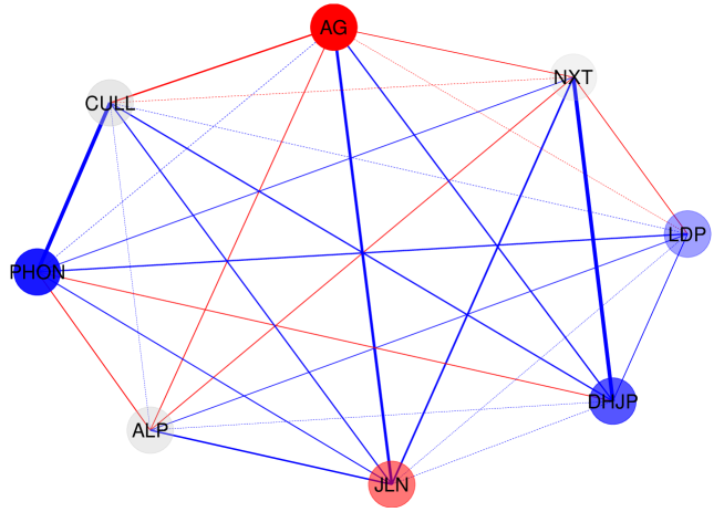
Figure 1: Visualization of the significance and interaction results from Tables 2 and 4. Descriptions of the various elements of the figure appear within the text.

We note that 5 out of the 8 bias elements are inferred to be significant different from zero, and 10 out of the 28 interaction elements are inferred to be significantly different to zero. Given such a large number of simultaneous hypothesis tests, and such a large number of significant results, it is prudent to control for the potentially inflated numbers of false positives that may occur. Towards this goal, we choose to employ the paradigm of false discovery rate (FDR) control, as considered by Benjamini and Hochberg (1995). Since there are potential dependencies between the hypotheses that are tested, we choose to use the method of Benjamini and Yekutieli (2001), which is able to control the FDR in the presence of dependencies between hypotheses. We adjust the $p\text{-values}$ so that we may control the FDR via the method of Benjamini and Yekutieli (2001) via the p.adjust function in R. The adjusted $p\text{-values}$ can be interpreted as per the unadjusted $p\text{-values}$, albeit with cutoffs indicating rejection of hypotheses at some level of FDR control rather than the usual significance level, instead. The FDR adjusted version of Table 4 is displayed in Table 6.

Table 6: Sub-table A contains the FDR-adjusted $p\text{-value}$ for the tests that each bias vector element is equal to zero. Sub-table B contains the FDR-adjusted $p\text{-value}$ for the tests that each interaction matrix element is equal to zero.

A
Party	ALP	AG	NXT	PHON	LDP	JLN	DHJP	CULL
$\text{adj-}p$	1.88E-01	1.24E-05	8.52E-01	6.41E-03	8.45E-02	2.13E-02	2.13E-02	7.45E-01
B
Party	ALP	AG	NXT	PHON	LDP	JLN	DHJP
AG	9.84E-01
NXT	1.00E+00	1.00E+00
PHON	7.45E-01	1.00E+00	1.00E+00
LDP	1.00E+00	1.00E+00	1.00E+00	2.33E-01
JLN	1.29E-01	1.84E-03	7.96E-02	6.75E-01	1.00E+00
DHJP	1.00E+00	2.33E-01	4.17E-05	1.00E+00	1.00E+00	1.00E+00
CULL	1.00E+00	1.75E-01	1.00E+00	4.17E-05	1.00E+00	2.82E-01	2.33E-01

We observe that the FDR-adjusted $p\text{-values}$ indicate that, when controlling at the $5\%$ FDR, we would only reject 4 out of the 8 hypotheses regarding the bias elements, and only 3 out of 28 hypotheses relating to the interaction matrix. Thus, the use of FDR adjustment significantly reduces our power for detecting an interesting interaction.

It is well-known that the method of Benjamini and Yekutieli (2001) is very conservative, especially when there is a potentially large number of hypotheses where the null hypotheses are false. That is, when there are many false null hypotheses, the method of Benjamini and Yekutieli (2001) controls the FDR at a level that is substantially smaller than the specified cutoff level (i.e. $5\%$, above). To counteract this effect, it is not uncommon to utilize an FDR cutoff that is larger than the significance level $\alpha$, that would otherwise be used in a significance test. Thus, we choose to control the FDR at the $10\%$ level, which yields 5 out of 8 rejected bias elements, and 4 out of 28 rejected interaction elements.

As with Figure 1, we summarize the results of Tables 2 and 6 in Figure 2. We can interpret the diagram as follows, with hypotheses declared rejected or otherwise at the $10\%$ level of FDR control. Each node is colored blue, grey, or red, depending on whether the hypothesis of the estimated bias of the corresponding party is rejected with a positive bias, not rejected, or rejected with a negative bias, respectively. Each node is more opaque if the absolute value of the estimated bias is higher.

The edges connecting each node are either solid or dashed. A solid edge indicates that the corresponding hypothesis of the interaction between the two connected parties is rejected, and a dashed edge indicates that the hypothesis is not. An edge is colored blue if the interaction between the two parties is positive, and a red edge indicates a negative interaction. The edge thickness is directly proportional to the negative logarithm of the adjusted $p\text{-value}$ of the corresponding interaction between the two parties.

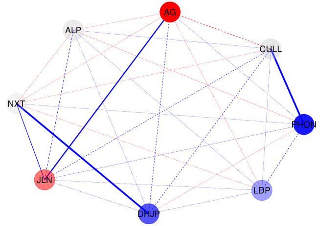
Figure 2: Visualization of the FDR control and interaction results from Tables 2 and 6. Descriptions of the various elements of the figure appear within the text.

4.1 Discussions

We begin by discussing the results from Table 5. The ALP is the oldest of the Australian parties and has a continuous existence since 1891, where it has either governed or acted as the opposition (Weller and Fleming, 2003). As opposition, it is unsurprising that the ALP should have a low marginal probability of agreement with the government. It is also unsurprising that AG has a low marginal probability of agreement with the Government, since it is a progressive party with ideologies that are antithetical to neo-liberalism and conservatism of the governing LNP (see, e.g., Miragliotta, 2010 and Mendes, 1998 regarding the AG and LNP, respectively). Next, the high rates of agreement with the government, of PHON, LDP, and CULL is also not surprising since PHON is largely a nationalistic and conservative party (Grant et al., 2019) and the LDP is self-described as an economically neo-classically liberal and libertarian party (cf. www.ldp.org.au/our_philosophy).

The low probability of agreement between JLN and the Government is somewhat surprising since JLN is seen as a conservative party (cf. Wood et al., 2018). Both NXT and DHJP are largely personality-based parties, with NXT being self identified as being a centralist party that seeks to break the duopoly of the ALP and LNP (Kefford, 2018). It is therefore unsurprising that NXT has an agreement probability that is close to $50\%$. On the other hand, DHJP ran a single-issue policy platforms centered around judicial reform (cf. www.justiceparty.com.au/our-policies), and thus we had no a priori expectations regarding the relationship between DHJP and the conservative Government. It is therefore of great interest to observe that DHJP is generally amenable to the position of the Government.

Next, we discuss the results from Tables 2 and 6, via the aid of Figure 2. We observe that upon controlling the FDR at the $10\%$ level and in the presence of the interactions, PHON, LDP, and DHJP are biased towards agreement with the Government, and AG and JLN are biased towards disagreement with the Government. We also observe that ALP, NXT, and CULL have no bias either way.

The biased positions of PHON and LDP towards agreement, and AG towards disagreement is not surprising, as has been discussed above. However, the bias against the Government by JLN is surprising, but is in correspondence with what we observed from Table 5. The bias towards agreement by DHJP is also in correspondence with the above $50\%$ marginal rate of agreement, that was observed in Table 5.

Of the three parties that exhibit a lack of bias, when controlled at the $10\%$ FDR level, the result for NXT and CULL are not surprising. As we have already discussed, NXT and CULL are both parties that are heavily driven by interactions with other parties (PHON and DHJP, respectively). Given the strong bias towards voting for the government of both PHON and DHJP, it is unsurprising that these strong interactions drive the marginal rate of agreement of both NXT and CULL, upwards.

It is however surprising that ALP should lack a bias, given that they are the opposition to the Government. We observe from Table 4 that the downward bias from the ALP is significant at the $\alpha=0.1$ level. We thus propose that the lack of rejection of the hypothesis for the bias element associated with the ALP may be due to sampling error. Another potential reason is that the ALP and LNP have had a history of voting together on issues such as defense, in the spirit of bipartisanship (see, e.g., Murphy, 2014 and Carr, 2015). It is a matter of debate as to whether this bipartisanship represents a lack of ideological difference between the two parties or whether the behavior is merely pragmatic in nature.

We now discuss the interactions between the parties. The least surprising of the interactions is that between PHON and CULL, given that they voted the same way on all 12 Senate questions. Next, the positive interaction between AG and JLN is perhaps due to the fact that Jacqui Lambie, along with two of the nine AG Senators are Tasmanian (cf. Evans, 2016, Tab. 1 and Bolwell and Eccleston, 2017), and thus are allied in voting in a manner that best benefits the state.

The positive interaction between NXT and JLN is more obvious as both Nick Xenophon as the two parties had agreed to an alliance prior to the 2016 election (cf. Atkin, 2015). Lastly, the positive interaction between NXT and DHJP may come down to the two entities having formed an alliance in the Senate (cf. Hinch, 2016).

5 Conclusion

We had set out with the aim to quantitatively analyze the degree to which each of the non-government parties of the Senate of the 45th Australian Parliament were pro- or anti-Government, and the degree to which the votes of each of the non-government Senate parties were in concordance or discordance with one another. Using the FVBM as an inferential vehicle, we were able to satisfactorily achieve both of the stated aims.

Our investigation centered around the analysis of the Senate data, that were described in Section 3. We found that the use of an FVBM, fitted via MPLE, provided a good fit to the data. Furthermore, analysis of these data revealed voting patterns that were largely supported by the literature and external sources. In particular, our analyses of whether parties were pro- or anti-Government yielded results that were in correspondence with the ideological positions of the assessed parties. Furthermore, identified interactions between parties were in general accordance with identifiable parliamentary alliances. Thus, we conclude that our FVBM methodology was successfully applied for the analysis of the Senate data, and may be applicable to similarly structured data sets.

A number of possible future directions for our research have been identified. Firstly, we may consider the case of dependent observations, and allow for autoregressive structures between voting events that follow sequentially from each other. Secondly, we may allow for the bias and interaction parameter elements of the FVBM to be parametrizable by covariates, in order to produce a richer class of models. Thirdly, we may substitute the FDR control procedure with a regularization procedure, instead, using penalizations such as the LASSO of Tibshirani (1996). Such a procedure may be more powerful in identifying relationships between political entities. Finally, given the parametric construction of the FVBM, it is conceivable that we may be able to conduct missing data imputation and parameter estimation, simultaneously. The derivation of such an algorithm, as well as progress with respect to the other future directions, would require significant further technical developments, which cannot be achieved within the length and scope constraints of this manuscript.

Appendix

Sensitivity of the analysis to $k$ in $k\text{-nearest neighbor}$ imputation

As discussed in Section 3.1, $k\text{-nearest neighbor}$ imputation was used to account for missing data in our Senate voting data set, where $k=3$. The choice of $k=3$ was made based on a recommendation by Beretta and Santaniello (2016), who observed that the choice provided a good balance between precision and generalizability.

In order to assess whether our analyses was sensitive to the choice, we also conducted $k=1$ and $k=5$ imputation, and fitted FVBMs to our differently imputed data. We reproduce Tables 2 and 6 for the two alternative choices of $k$. Tables 7 and 8 contain the MPLE and FDR-adjusted $p\text{-values}$, computed after $1\text{-nearest neighbor}$ imputation. Tables 9 and 10 contain the MPLE and FDR-adjusted $p\text{-values}$, computed after $5\text{-nearest neighbor}$ imputation.

Table 7: Sub-table A contains the estimated values of the bias vector (i.e. $\tilde{\bm{b}}_{n}$), computed after $1\text{-nearest neighbor}$ imputation. Sub-table B contains the corresponding estimated values of the unique elements of the interaction matrix (i.e $\tilde{\bm{M}}_{n}$).

A
Party	ALP	AG	NXT	PHON	LDP	JLN	DHJP	CULL
Bias	-0.250	-1.031	-0.150	1.026	0.180	-0.636	0.650	-0.352
B
Party	ALP	AG	NXT	PHON	LDP	JLN	DHJP
AG	-0.306
NXT	-0.209	-0.272
PHON	-0.345	0.065	0.327
LDP	0.093	0.062	-0.103	0.654
JLN	0.498	0.752	0.405	0.506	-0.069
DHJP	0.044	0.594	0.672	-0.525	0.269	0.067
CULL	0.014	-0.743	-0.049	1.225	0.169	0.412	0.746

Table 8: Sub-table A contains the FDR-adjusted $p\text{-value}$ for the tests that each bias vector element is equal to zero, computed after $1\text{-nearest neighbor}$ imputation. Sub-table B contains the corresponding FDR-adjusted $p\text{-value}$ for the tests that each interaction matrix element is equal to zero.

A
Party	ALP	AG	NXT	PHON	LDP	JLN	DHJP	CULL
$\text{adj-}p$	5.12E-01	1.83E-05	1.00E+00	2.69E-03	8.86E-01	6.92E-03	2.60E-02	8.45E-01
B
Party	ALP	AG	NXT	PHON	LDP	JLN	DHJP
AG	2.87E-01
NXT	6.98E-01	1.00E+00
PHON	6.98E-01	1.00E+00	1.00E+00
LDP	1.00E+00	1.00E+00	1.00E+00	5.00E-02
JLN	1.73E-03	6.92E-05	1.54E-01	2.87E-01	1.00E+00
DHJP	1.00E+00	1.93E-01	9.47E-05	6.98E-01	4.86E-01	1.00E+00
CULL	1.00E+00	1.54E-01	1.00E+00	6.92E-05	1.00E+00	2.87E-01	1.93E-01

Table 9: Sub-table A contains the estimated values of the bias vector (i.e. $\tilde{\bm{b}}_{n}$), computed after $5\text{-nearest neighbor}$ imputation. Sub-table B contains the corresponding estimated values of the unique elements of the interaction matrix (i.e $\tilde{\bm{M}}_{n}$).

A
Party	ALP	AG	NXT	PHON	LDP	JLN	DHJP	CULL
Bias	-0.326	-1.077	-0.185	0.830	0.532	-0.555	0.751	-0.433
B
Party	ALP	AG	NXT	PHON	LDP	JLN	DHJP
AG	-0.209
NXT	-0.197	-0.256
PHON	-0.355	0.058	0.349
LDP	0.149	0.121	-0.199	0.532
JLN	0.312	0.623	0.421	0.358	0.033
DHJP	0.068	0.593	0.791	-0.488	0.050	0.093
CULL	0.053	-0.754	-0.119	1.226	0.314	0.395	0.824

Table 10: Sub-table A contains the FDR-adjusted $p\text{-value}$ for the tests that each bias vector element is equal to zero, computed after $5\text{-nearest neighbor}$ imputation. Sub-table B contains the corresponding FDR-adjusted $p\text{-value}$ for the tests that each interaction matrix element is equal to zero.

A
Party	ALP	AG	NXT	PHON	LDP	JLN	DHJP	CULL
$\text{adj-}p$	1.88E-01	2.45E-05	1.00E+00	3.45E-02	3.45E-02	2.82E-02	2.82E-02	5.90E-01
B
Party	ALP	AG	NXT	PHON	LDP	JLN	DHJP
AG	9.20E-01
NXT	9.97E-01	1.00E+00
PHON	9.13E-01	1.00E+00	1.00E+00
LDP	1.00E+00	1.00E+00	1.00E+00	2.27E-01
JLN	1.48E-01	2.05E-03	7.37E-02	9.13E-01	1.00E+00
DHJP	1.00E+00	2.27E-01	2.97E-05	1.00E+00	1.00E+00	1.00E+00
CULL	1.00E+00	1.64E-01	1.00E+00	2.07E-04	1.00E+00	2.98E-01	2.27E-01

From Tables 7 and 9, we observe that, although there are small deviations in the value of the MPLE estimates, the direction of the estimated biases and interactions are the same as those that are reported in Table 2. The results from Table 10 show that the conclusions drawn with FDR controlled at the $10\%$ level, under $5\text{-nearest neighbor}$ imputation, is the same as the conclusions that can be drawn from Table 6.

We observe that there are some small differences in conclusions, when drawing inference with FDR controlled at the $10\%$ level, between Tables 6 and 8. Firstly, we no longer reject the assumption of no bias for LDP, and we no longer infer interactions between JLN and NXT. We reject an additional two interaction hypotheses, however, between ALP and JLN, and between PHON and LDP. None of these changes contradict the conclusions that we have drawn in Section 4.

Simulation results from Beretta and Santaniello (2016) show that $1\text{-nearest neighbor}$ imputation can often be inaccurate, when compared to larger values of $k$. However, the simulations of Beretta and Santaniello (2016) were for a real-valued regression problem, rather than a binary PMF estimation problem. Thus, we are cautious to make any stronger claims regarding the relevance of their results to our modeling problem. We believe that a model-based approach that conducts imputation and estimation, simultaneously, may resolve our problem of having to choose tune our imputation scheme. However, as we have already mentioned in our conclusion, this would constitute a significant amount of new work that lies outside the scope of this manuscript.

References

- Ackley et al. [1985] D H Ackley, G E Hinton, and T J Sejnowski. A learning algorithm for Boltzmann machines. Cognitive Science, 9:147–169, 1985.
- Arnold and Strauss [1991] B C Arnold and D Strauss. Pseudolikelihood estimation: some examples. Sankhya B, 53:233–243, 1991.
- Atkin [2015] M Atkin. Nick Xenophon and Jacqui Lambie agree to preference deal for next federal election, 2015. URL www.abc.net.au/news/2015-09-07/nick-xenophon-jacqui-lambie-federal-election-alliance/6755654.
- Begg [2017] M Begg. The citizenship saga. Institute of Public Affairs Review: A Quarterly Review of Politics and Public Affairs, 69:30–33, 2017.
- Benjamini and Hochberg [1995] Y Benjamini and Y Hochberg. Controlling the false discovery rate: a practical and powerful approach to multiple testing. Journal of the Royal Statistical Society Series B, 57:289–300, 1995.
- Benjamini and Yekutieli [2001] Y Benjamini and D Yekutieli. The control of the false discovery rate in multiple testing under dependency. Annals of Statistics, 29:1165–1188, 2001.
- Beretta and Santaniello [2016] L Beretta and A Santaniello. Nearest neighbor imputation algorithms: a critical evaluation. BMC Medical Informatics and Deicision Making, 16(Suppl 3):74, 2016.
- Bolwell and Eccleston [2017] D Bolwell and R Eccleston. Tasmania July to December 2016. Australian Journal of Politics and History, 63:320–327, 2017.
- Boos and Stefanski [2013] D D Boos and L A Stefanski. Essential Statistical Inference: Theory And Methods. Springer, New York, 2013.
- Carr [2015] A Carr. Is this the end of defence bipartisanship?, 2015. URL https://www.abc.net.au/news/2015-08-19/carr-the-end-of-defence-bipartisanship/6708422.
- Corcoran and Dickenson [2010] R Corcoran and J Dickenson. A Dictionary of Australian Politics. Allen and Unwin, Adelaide, 2010.
- Cox [1972] D R Cox. The analysis of multivariate binary data. Journal of the Royal Statistical Society C, 21:113–120, 1972.
- Desmarais and Crammer [2010] B A Desmarais and S J Crammer. Consistent confidence intervals for maximum pseudolikelihood estimators. In Proceedings of the Neural Information Processing Systems 2010 Workshop on Computational Social Science and the Wisdom of Crowds, 2010.
- Evans [2016] H Evans. ODGERS’ Australian Senate Practice. Commonwealth of Australia, Canberra, 2016.
- Franzin et al. [2017] A Franzin, F Sambo, and B Di Camillo. bnstruct: an R package for Bayesian network structure learning in the presence of missing data. Bioinformatics, 33:1250–1252, 2017.
- Gauja et al. [2018] A Gauja, P Chen, J Curtin, and J Pietsch, editors. Double Disillusion: the 2016 Australian Federal Election. ANU Press, Acton, 2018.
- Graham et al. [1989] R L Graham, D E Knuth, and O Patashnik. Concrete Mathematics. Addison-Wesley, Reading, 1989.
- Grant et al. [2019] B Grant, T Moore, and T Lynch, editors. The Rise of Right-Popularism: Pauline Hanson’s One Nation and Australian Politics. Springer, Singapore, 2019.
- Hinch [2016] D Hinch. Hinch’s Senate Diary: beware the Gang of Four, 2016. URL www.crikey.com.au/2016/11/24/derryn-hinch-forms-alliance-with-nick-xenophon-team.
- Hobbs et al. [2018] H Hobbs, S Pillai, and G Williams. The disqualification of dual citizens from Parliament: three problems and a solution. Alternative Law Journal, 43:73–80, 2018.
- Hunter and Lange [2004] D R Hunter and K Lange. A tutorial on MM algorithms. The American Statistician, 58:30–37, 2004.
- Hyvarinen [2006] A Hyvarinen. Consistency of pseudolikelihood estimation of fully visible Boltzmann machines. Neural Computation, 18:2283–2292, 2006.
- Jones and Nguyen [2018] A T Jones and H D Nguyen. BoltzMM: Boltzmann machines with MM algorithms. The Comprehensive R Archive Network, 2018. URL https://CRAN.R-project.org/package=BoltzMM.
- Kefford [2018] G Kefford. The minor parties’ campaigns. In A Gauja, P Chen, J Curtin, and J Pietsch, editors, Double Disillusion: the 2016 Australian federal election. ANU Press, Acton, 2018.
- Lauritzen [1996] S L Lauritzen. Graphical Models. Oxford University Press, Oxford, 1996.
- Le Roux and Bengio [2008] N Le Roux and Y Bengio. Representational power of restricted Boltzmann machines and deep belief networks. Neural Computation, 20:1631–1649, 2008.
- Lindsay [1988] B Lindsay. Composite likelihood methods. Contemporary Mathematics, 8:221–239, 1988.
- Mendes [1998] P Mendes. From Keynes to Hayek: the social welfare philosophy of the liberal party of Australia, 1983–1997. Policy, Organisation and Society, 15:65–87, 1998.
- Miragliotta [2010] N Miragliotta. From local to national: explaining the formation of the Australian Green Party. Party Politics, 18:409–425, 2010.
- Molenberghs and Verbeke [2005] G Molenberghs and G Verbeke. Models For Discrete Longitudinal Data. Springer, New York, 2005.
- Murphy [2014] K Murphy. Anthony Albanese: Labor has gone too far in support of national security, 2014. URL https://www.theguardian.com/australia-news/2014/oct/12/anthony-albanese-labor-has-gone-too-far-in-supporting-national-security-laws.
- Nguyen [2017] H D Nguyen. An introduction to MM algorithms for machine learning and statistical estimation. WIREs Data Mining and Knowledge Discovery, 7:e1198, 2017.
- Nguyen [2018] H D Nguyen. Near universal consistency of the maximum pseudolikelihood estimator for discrete models. Journal of the Korean Statistical Society, 47:90–98, 2018.
- Nguyen and Wood [2016a] H D Nguyen and I A Wood. Asymptotic normality of the maximum pseudolikelihood estimator for fully visible Boltzmann machines. IEEE Transactions on Neural Networks and Learning Systems, 27:897–902, 2016a.
- Nguyen and Wood [2016b] H D Nguyen and I A Wood. A block successive lower-bound maximization algorithm for the maximum pseudolikelihood estimation of fully visible Boltzmann machines. Neural Computation, 28:485–492, 2016b.
- Phillips and Kerr [2017] H C J Phillips and L Kerr. Western Australia July to December 2016. Australian Journal of Politics and History, 63:310–315, 2017.
- R Core Team [2016] R Core Team. R: a language and environment for statistical computing. R Foundation for Statistical Computing, 2016.
- Razaviyayn et al. [2013] M Razaviyayn, M Hong, and Z-Q Luo. A unified convergence analysis of block successive minimization methods for nonsmooth optimization. SIAM Journal of Optimization, 23:1126–1153, 2013.
- Remeikis [2017] Amy Remeikis. Rodney Culleton was never legally elected to Senate, High Court rules, 2017. URL https://www.smh.com.au/politics/federal/rodney-culleton-was-never-elected-to-senate-high-court-rules-20170203-gu4kfu.html.
- Stubbs [2017] M Stubbs. Ensuring loyalty to the public: the High Court’s decision to disqualify Day and Culleton from Parliament. Bulletin (Law Society of South Australia), 39:7, 2017.
- Tibshirani [1996] R Tibshirani. Regression shrinkage and selection via the Lasso. Journal of the Royal Statistical Society Series B, 58:267–288, 1996.
- Troyanskaya et al. [2001] O Troyanskaya, M Cantor, G Sherlock, P Brown, T Hastie, R Tibshirani, D Botstein, and R B Altman. Missing value estimation methods for DNA microarrays. Bioinformatics, 17:520–525, 2001.
- van der Vaart [1998] A van der Vaart. Asymptotic Statistics. Cambridge University Press, Cambridge, 1998.
- Weller and Fleming [2003] P Weller and J Fleming. The Commonwealth. In J Moon and C Sharman, editors, Australian Politics and Government: the Commonwealth, the States and the Territories. Cambridge University Press, 2003.
- Wood et al. [2018] D Wood, J Daley, and C Chivers. Australia demonstrates the rise of populism is about more than economics. Australian Economic Review, 51:399–410, 2018.
- Wright and Fowler [2012] B C Wright and P E Fowler, editors. House of Representatives Practice. Commonwealth of Australia, Canberra, 2012.