Efficient Search for Diverse Coherent Explanations

Abstract.

This paper proposes new search algorithms for counterfactual explanations based upon mixed integer programming. We are concerned with complex data in which variables may take any value from a contiguous range or an additional set of discrete states. We propose a novel set of constraints that we refer to as a “mixed polytope” and show how this can be used with an integer programming solver to efficiently find coherent counterfactual explanations i.e. solutions that are guaranteed to map back onto the underlying data structure, while avoiding the need for brute-force enumeration. We also look at the problem of diverse explanations and show how these can be generated within our framework.

1. Introduction

A fundamental tension exists between the high performance of machine learning algorithms and the notion of transparency (Lipton, 2016). The large complex models of machine learning are created by researchers and system builders looking to maximise their performance on real-world data, and it is precisely their size and complexity that allows them to fit to the data giving them such high-performance. At the same time such models are simply too complex to fit in their builders minds; and even the people that created the systems need not understand why they make particular decisions.

This tension becomes more apparent as we start using machine learning to make decisions that substantially alter people’s lives. As algorithms are used to make loan decision; to recommend whether or not some one should be released on parole; or to detect cancer, it is vital that not only are the algorithms used as accurate as possible, but also that they justify themselves in some way, allowing the subject of the decisions to verify the data used to make decisions about them, and to challenge inappropriate decisions

A common remedy to avoid this trade-off is to learn the complex function, and then fit simple models about datapoints providing human comprehensible approximations of the underlying function. While popular in the machine learning community, there are many challenges in conveying the quality of the approximation and the domain over which it is valid to a lay audience.

Another promising approach to explaining the incomprehensible models of machine learning lies in counterfactual explanations (Wachter et al., 2018; Lewis, 1973). This recent approach to explainablity bypasses the problem of describing how a function works and instead focuses on the data. Instead, counterfactual explanations attempt to answer the question “How would my data need to be changed to get a different outcome?”. Wachter et al. make the argument that there are three important use cases for explanation:

1. to inform and help the individual understand why a particular decision was reached,

2. to provide grounds to contest the decision if the outcome is undesired, and

3. to understand what would need to change in order to receive a desired result in the future, based on the current decision-making model.

and that counterfactual explanations satisfy all three.

Although making the case for the use of counterfactuals and showing how they could be effectively calculated for common classifiers, Wachter et al. left many technical questions unanswered. Of particular concern is the issue of how should we generate counterfactuals efficiently and reliably for standard classifiers.

This paper focuses on the technical aspects needed to generate coherent counterfactual explanations. Keeping the existing definition of counterfactual explanations intact, we look at how explanations can be reliably generated. We make two contributions:

1. Focusing on primarily the important problem of explaining financial decisions, we look at the most common case in which the classifier is linear (i.e. linear/logistic regression, SVM etc.) but the data has been transformed via a mix-encoding based upon 1-hot or dummy variable encoding. We present a novel integer program based upon a “mixed polytope” that is guaranteed to generate coherent counterfactuals that map back into the same form as the original data.

2. We provide a novel set of criteria for generating diverse counterfactuals and integrate them with our mixed polytope method.

Previously, Wachter et al. strongly made the case that diverse counterfactuals are important to informing a lay audience about the decisions that have been made, writing that: “…individual counterfactuals may be overly restrictive. A single counterfactual may show how a decision is based on certain data that is both correct and unable to be altered by the data subject before future decisions, even if other data exist that could be amended for a favourable outcome. This problem could be resolved by offering multiple diverse counterfactual explanations to the data subject.” but to date no one has proposed a concrete method for generating them.

We evaluate our new for mixed data approach on standard explainability problems, and the new FICO explainability dataset, where we show our fully automatic approach generates coherent and informative diverse explanations for a range of sample inputs.

2. Prior Work

The desire for explanations of how complex computer systems make decisions dates back to some of the earliest work on expert systems (Buchanan and Shortliffe, 1984). In the context of machine learning, much prior work has focused upon providing human-comprehensible approximations (typically either linear models (Ribeiro et al., 2016; Montavon et al., 2017; Shrikumar et al., 2016; Lundberg and Lee, 2017), or decision trees (Craven and Shavlik, 1996)) of the true decision making criteria. This fact that the simplified model is only an approximation of the true decision making criteria means that these methods avoid the trade-off between accuracy and explainablity discussed in the introduction, but also raises the question of how accurate these approximations really are.

These approximate models are either fitted globally (Craven and Shavlik, 1996; Martens et al., 2007; Sanchez et al., 2015) over the entire space of valid datapoints, or as a local approximation (Ribeiro et al., 2016; Montavon et al., 2017; Shrikumar et al., 2016; Lundberg and Lee, 2017) that only describes how decisions are made in the neighbourhood of a particular datapoint.

Another important class of explanations comes from “case-based reasoning” (Caruana et al., 1999; Kim et al., 2014) in which the method justifies the decision/score made by the algorithm by showing data points from the training set that the algorithm found similar in some sense.

Finally, there are methods for contrastive or counterfactual explanations that seek a minimal change such that the response of the algorithm changes e.g.

“You were denied a loan because you have an income of $30,000, if you had an income of $45,000 you would have been offered the loan.”

Martens and Provost (2013) was the first to propose the use of this technique in the context of removing words for website classification, while Wachter et al. (2018) proposed it as a general framework suitable for continuous and discrete data. Use of counterfactual explanations have strong support from the social sciences (Miller, 2017), and form part of the established philosophical literature on explanations (Lewis, 1973; Kment, 2006; Ruben, 2004). Others have called for the use of counterfactuals in explaining machine learning (Doshi-Velez et al., 2017). Finally, Binns et al. (2018) followed (Lim and Dey, 2009) in performing a user study of explanations. Binns et al. (2018) found evidence that users prefer counterfactual explanations over case-based reasoning.

For a more detailed review of the literature, please see (Mittelstadt et al., 2019).

Finally, concurrent with this work, (Ustun et al., 2019), have also proposed the generation of diverse counterfactuals using mixed integer programmes for linear models. However, they do not consider the case of complex data in which individual variables may take either a value from a continuous range, or one of a set of discrete values.

2.1. Formalising Counterfactual Explanations

We follow (Lewis, 1973) in describing a counterfactual as a “close possible world” in which a different outcome (or classifier response) occurs. In the context of classifier responses, we can formalise this as follows:

Given a datapoint $x$ , the closest counterfactual $x^{\prime}$ can then be found by solving the problem

(1) $$\arg\min_{x^{\prime}}\,\, d(x,x^{\prime})$$

(2) such that: $$f(x^{\prime})=c$$

where $d(\cdot,\cdot)$ is a distance measure, $f$ the classifier function and $c$ the classifier responses we desire.

This is a much looser definition of counterfactual than that used in the causal literature (e.g. Pearl (2000)) and some thought needs to go into the choice of distance function to make the counterfactuals found useful.

In the context of human comprehensible explanations, it is important that the change between the original datapoint, and the counterfactual is simple enough that a person can understand it, and that the way the datapoint is altered to generate the counterfactual should also be representative of the original dataset in some way.

To meet these objectives, Wachter et al. suggested making use of the $\ell_{1}$ norm, weighted by the inverse Median Absolute Deviation, which we write as $||\cdot||_{1,\text{MAD}}$. This has two noticeable advantages: (i) The counterfactuals found are typically sparse i.e. they differ from the original datapoint in a small number of factors, making the change easier to comprehend. (ii) In some limited sense the distance function is scale free, in that multiplying one dimension by a scalar will not alter the solution found, and robust to outliers.

Wachter et al. (2018) proposed solving this problem as a Lagrangian:

(3) $$\min_{x^{\prime}}\max_{\lambda} ||x-x^{\prime}||_{1,\text{MAD}}+\lambda(f(x)-c)^{2}$$

As the term $\lambda$ tends to infinity this converges to a minimiser of $||x-x^{\prime}||_{1,\text{MAD}}$ that satisfies $f(x)=c$ or at least is a local minima of $(f(x)-c)^{2}$. Stability is a major concern when using the Lagrangian approach to generating counterfactual explanations. It is important that the counterfactuals generated do what they set out to do and satisfy the constraint $f(x^{\prime})\leq 0$ to within a very tight tolerance. For this to happen the value $\lambda$ much be sufficiently large and this induces stability issues (Wright and Nocedal, 1999). Moreover, the shape of the objective for is reminiscent of pathological optimisation problems. Noticeably, for large $\lambda$ the objective forms a deep narrow valley around the decision boundary similar to a high-dimensional analogue of the Rosenbrock or ‘banana’ function (Rosenbrock, 1960), while the sparsity of the solution found means that the minima occurs at gradient discontinuities in the objective function.

To avoid these issues we preserve the original formulation of equation (1), with explicit constraints. We show how this problem can be formulated as a linear programme when $f$ is linear and distance function $d$ takes the form of a weighted $\ell_{1}$ norm. Where they occur, binary constraints (such as this variable must take only values $0$ or $1$) are treated as integer constraints and our final formulation is efficiently solved using a Mixed Integer Program Solver.

3. Coherent Counterfactuals on Mixed Data

We now outline our procedure for generating coherent counterfactual explanations for linear classifiers, including logistic and linear regression and SVMs, defined over complex datasets where the variables may take any value from a contiguous range or an additional set of discrete states,

For such mixed data the notion of distance becomes problematic. For example, in the FICO dataset, one of the variables that measures “Months Since Most Recent Delinquency” may take either a non-negative value corresponding to the number of months, or a set of special values:
$-7$ “Condition not Met (e.g. No Inquiries, No Delinquencies)” $-8$ “No Usable/Valid Trades or Inquiries” or $-9$ “No Bureau Record or No Investigation”.

Beyond the computational challenges in searching over all valid values for all sets of variables, it is apparent that the change from special value $-7$ to $-8$ is fundamentally different from the shift between “7 months since most recent delinquency” and “8 months since most recent delinquency”.

A common trick among applied statisticians when training predictors on this kind of data is to augment it using a variant of the one-hot (or dummy variable) encoding. Here, a variable $x_{i}$ that takes either a contiguous value, or one $k$ discrete states is replaced by $k+1$ variables. The first of these variable takes either the contiguous value, if $x_{i}$ is in the contiguous range or a fixed response $F_{i}$ (typically 0) if $x_{i}$ is in a discrete state. The remaining $k$ variables $d_{i,1},\ldots,d_{i,k}$ are indicator variables that take value $1$ if $x_{i}$ is in the appropriate discrete state and $0$ otherwise. A linear classifier can be trained on these encoded datapoints instead of the original data with substantially higher performance.

The challenge with using such embedding into higher-dimensional spaces, and then computing counterfactuals in the embedding space, is that the extra degrees of freedom allow nonsense states (for example turning all indicator variables on) which do not map back into the original data space. We show how a small set of linear constraints can avoid many of these failures, and by combining it with simple integer constraints for the indicator variables guarantee that the counterfactual found is coherent. We will refer to the space enclosed by these linear constraints as the “mixed polytope”.

We refer to a particular datapoint a decision has been made about as $x$ and it’s individual components as $x_{i}$. We write $c_{i}$ for the $i^{\text{th}}$ contiguous variable that can take values in the range $[L_{i},U_{i}]$ and use $d_{i,j}$ for the $j^{\text{th}}$ component of the $i^{\text{th}}$ set of indicator variables that has value $1$ if $x_{i}$ is taking the $j^{\text{th}}$ discrete value. To make optimisation tractable under these constraints we assume that this decision has been made by a linear function $f(x)=w\cdot x+b$.

The mixed polytope of variable $i$ then is described by the linear constraints:

(4) $$\sum_{j}d_{i,j}+d_{i,c}=1$$

(5) $$F_{i,}-l_{i}+u_{i}=c_{i}$$

(6) $$0\leq l_{i}\leq(L_{i}-F_{i})d_{i,c}$$

(7) $$0\leq r_{i}\leq(R_{i}-F_{i})d_{i,c}$$

(8) $$d_{i,j}\in[0,1]\qquad\forall j$$

where $d_{i,c}$ is an additional indicator value that shows that variable $v$ is takes a contiguous value. It is immediately obvious that if the variables $d_{i,j}$ are binary, i.e. take values $\{0,1\}$, then any vector $[c_{i},d_{i,1},\ldots,d_{i,k}]$ that lies in the mixed polytope is consistent with a standard mixed encoding from a consistent state. Moreover, the polytope is tight in so much as optimising a linear objective defined directly over the variables $d$ and $c$ would result in a valid solution. However, we are unable to take advantage of this, as the additional constraint on the value of $f(x)$ further constrains the polytope and potentially allows for fractional optimal solutions if $d_{i}$ is not forced to be binary. We are now well placed to write down an Integer Program to generate counterfactuals. We write $\hat{x}$ for the mixed encoding of datapoint $x$ and assume that our classifier is linear in the embedding space.

We seek:

(9) $$\arg\min_{x^{\prime}} ||\hat{x}-x^{\prime}||_{1,w}$$

(10) such that: $$f(x^{\prime})\leq 0$$

(11) $$x^{\prime}\text{ lies on the mixed polytope}$$

(12) $$d_{i,j}\in\{0,1\}\qquad\forall i,j$$

where $||\cdot||_{1,w}$ is a weighted $\ell_{1}$ norm with the weights to be discussed later. Note that we now use the constraint $f(x)\leq 0$, rather than $f(x)=0$ as it is possible that changing the state of one of the discrete variables will take us over the boundary rather than up to it.

This can be expanded into a linear program. As $f$ is a linear classifier we can split it into linear sub-functions over the discrete and contiguous values ($d$ and $c$ respectively) and rewrite it as $f(x^{\prime})=a\cdot c+\sum_{i}a_{i}^{\prime}\cdot d_{i}+b$ allowing $f(x^{\prime})\leq 0$ to be replaced with the linear constraint. The objective $\min_{c}||\hat{x}_{c}-c||_{1,w}$ can be made linear using the standard transformation:

(13) $$\min_{c}||\hat{x}-c||_{1,w}= \min_{c,g,h}\sum_{i}(g_{i}+h_{i})$$

(14) such that: $$0\leq g_{i},\qquad\hat{x_{i}}-c{}_{i}\leq g_{i}\qquad\forall i$$

(15) $$0\leq h_{i},\qquad x^{\prime}_{i}-c_{i}\leq h_{i}\qquad\forall i$$

Putting this all together it gives us the following program

(16) $$\arg\min_{c,d,g,h} w\cdot(g+h)+\sum_{i}w_{i}^{\prime}\cdot(d_{i}-\hat{d_{i})}$$

(17) such that: $$a\cdot(g+h)+\sum_{i}a_{i}^{\prime}\cdot d_{i}+b\leq 0$$

(18) $$0\leq g_{i},\qquad\hat{x_{i}}-c{}_{i}\leq g_{i}\qquad\forall i$$

(19) $$0\leq h_{i},\qquad c{}_{i}-\hat{x}_{i}\leq h_{i}\qquad\forall i$$

(20) mixed polytope conditions hold

(21) $$d_{i,j}\in\{0,1\}\qquad\forall i,j$$

The encoding in equation (13) used for the continuous variables is not needed for the discrete variables, as owing to their binary nature, we can simply choose the sign of $w^{\prime}$ appropriately to penalise switching away from the state of $\hat{d}_{i}$. These equations can be given to a standard MIPS solver, such as Gurobi Optimization (2018), allowing coherent counterfactuals to be automatically generated.

⬇ You got score ’good’. One way you could have got score ’bad’ instead is if: ExternalRiskEstimate had taken value 63 rather than 74 Another way you could have got score ’bad’ instead is if: MSinceMostRecentDelq had taken value 15 rather than -7. ⬇ You got score ’good’. One way you could have got score ’bad’ instead is if: ExternalRiskEstimate had taken value 57 rather than 69 Another way you could have got score ’bad’ instead is if: NetFractionRevolvingBurden had taken value 41 rather than 0 Another way you could have got score ’bad’ instead is if: NumInqLast6M had taken value 4 rather than 2 Another way you could have got score ’bad’ instead is if: NumSatisfactoryTrades had taken value 27 rather than 41 Another way you could have got score ’bad’ instead is if: AverageMInFile had taken value 49 rather than 63; NumInqLast6Mexcl7days had taken value 0 rather than 2 Another way you could have got score ’bad’ instead is if: ExternalRiskEstimate had taken value -9 , rather than 69 Another way you could have got score ’bad’ instead is if: NumSatisfactoryTrades had taken value -9, rather than 41 Another way you could have got score ’bad’ instead is if: PercentTradesNeverDelq had taken value -9, rather than 95 ⬇ You got score ’bad’. One way you could have got score ’good’ is if: ExternalRiskEstimate took value 72 rather than -9

⬇ You got score ’bad’. One way you could have got score ’good’ instead is if: MSinceMostRecentDelq had taken value -7, rather than 3; MSinceMostRecentInqexcl7days had taken value 14 rather than 0 Another way you could have got score ’good’ instead is if: ExternalRiskEstimate had taken value 66 rather than 61; MSinceMostRecentInqexcl7days had taken value -8, rather than 0 Another way you could have got score ’good’ instead is if: NumSatisfactoryTrades had taken value 35 rather than 26; NumInqLast6M had taken value 0 rather than 1; NetFractionRevolvingBurden had taken value -9 rather than 57 Another way you could have got score ’good’ instead is if: PercentInstallTrades had taken value -9, rather than 57; NetFractionRevolvingBurden had taken value 0 rather than 57 Another way you could have got score ’good’ instead is if: NumInqLast6Mexcl7days had taken value 6 rather than 1; NumRevolvingTradesWBalance had taken value -9, rather than 6 Another way you could have got score ’good’ instead is if: AverageMInFile had taken value 238 rather than 86 Another way you could have got score ’good’ instead is if: MaxDelqEver had taken value -9, rather than 6; PercentInstallTrades had taken value 40 rather than 57; NumInqLast6M had taken value -9, rather than 1; NumRevolvingTradesWBalance had taken value 0 rather than 6 Another way you could have got score ’good’ instead is if: MSinceMostRecentDelq had taken value 83 rather than 3; MaxDelqEver had taken value 5 rather than 6; NetFractionInstallBurden had taken value -9, rather than 67; NumBank2NatlTradesWHighUtilization had taken value -9, rather than 2

Table 1. Two explanations for different pieces of data leading to a ‘good’ result on the FICO challenge (left, top) one of the few short explanations for ‘bad’ (left, bottom) on and a typical explanations for a datapoint scored as ‘bad’ (right).

3.1. Choices of Parameter

The solution found depends strongly upon the choice of parameters $w$ and $f$, which can be adjusted given better knowledge of the problem or what the explanations found should look like. Here we present some simple heuristics that give good results in practice.

Choice of $w$

We follow Wachter et al. in the use of the inverse median absolute deviation (MAD) for $w$ with some small modifications. We consider the contiguous and discrete values separately and generate the inverse MAD for contiguous regions by discarding datapoints that take one of the given discrete labels.

For the discrete labels, the measure of inverse MAD is inappropriate for any distribution over binary labels as the median absolute deviation over any distribution of binary labels is always zero. With only two possible states, the median will coincide with the mode and therefore the median of the absolute deviation will be zero. Instead, for binary variables we replace the MAD with the standard deviation over the data multiplied by a normalising constant $k=\Phi^{-1}(3/4)\approx 1.48$ to make it commensurate with the use of MAD elsewhere. We use $m$ to refer to these choices of weights.

Given $m$, we set the $w=m$, for all parameters penalising changes in the contiguous region of data . For the parameters $w^{\prime}$ that govern the cost of transitions from discrete states, we adapt $w^{\prime}$ depending on the value taken by the original datapoint we are seeking counterfactuals for. We wish transitions to any new discrete state to be penalised by the scaled inverse standard deviation associated with that state, while a transition away from a current discrete state to the contiguous region should be penalised by the scaled inverse standard deviation of the current state. We achieve this as follows: Given the scale parameters $m^{\prime}$, we set $w^{\prime}_{i,c}=0$ and if $x_{i}$ is currently in discrete state $i$, set $w_{j}:=m_{j}-m_{i}$ for all $j\neq i$ and final set $m_{i}:=-w_{i}$. This has the required properties.

Choice of $F_{i}$

Although we introduced the variable $F_{i}$ in the context of training the model, it can also be adjusted on a per-explanation basis, providing the intercept value $b$ is also altered to compensate. We choose the value $F_{i}$ in such a way that when $\hat{x}_{i}$ is in the contiguous range, it does not incur an additional penalty to transitioning to a discrete state. This is done setting $F_{i}:=x_{i}$. On the other-hand, when $\hat{x}_{i}$ takes a discrete value, we wish to ensure that transitioning to the contiguous range gives you a representative and typical value without incurring an additional cost. This is done by setting $F_{i}=\text{median}(X_{i})$.

4. Diverse Explanations

In the original paper of (Wachter et al., 2018) the authors note that diverse counterfactual explanations may often be useful – if someone wishes to improve their credit score, the first route to altering their data that you suggest may not be the useful for them, and another explanation would be more useful. Equally, if no other explanation exists, this too is valuable information for that person.

Wachter et al. suggested local optima might be one source of diversity. For linear classifiers their objective (3) is convex in $x^{\prime}$ for any choice of $\lambda$, and for problems of this particular form, only one minima exists.

Instead we take an different approach and induce diversity by restricting the state of variables altered in previously generated counterfactuals. This is done by following a obeying a simple set of rules which we give in the following paragraph.

Diversity constraints:

If a particular discrete state has been selected in a counterfactual but not in the original data we prohibit the transition to that state, but allow transitions to other discrete states by the same variable. If the counterfactual alters a discrete state to one in the contiguous range we prohibit that transition, while if it alters an already contiguous state to a new contiguous value we prohibit altering the contiguous state but allow transitions to one of the discrete states.

Each constraint is added individually, and if the addition of a new constraint means that the mixed integer program can no longer be satisfied, the constraint is immediately removed. The process terminates when the new counterfactual explanations generated is the same as the previous explanation.

Sample outputs of the entire procedure are discussed in the following section.

5. Experiments

To demonstrate the effectiveness of our approach, we generate diverse counterfactuals on a range of problems. All explanations generated will be human readable text that show the sparse changes needed. All text will take the form:

⬇

You got score ____.

One way you could have got score ____ is if:

____ took value ____ rather than ____

Another way you could have got score ____ is if:

____ had taken value ____ rather than ____

where the blanks are completed automatically. The list of explanations will be naturally ranked by their weighted $\ell_{1}$ distance from the original datapoint as they are computed by greedily adding constraints. For completeness, we show a full list of explanations as they are generated. If the generated counterfactuals are to be offered to consumers, this list should be truncated, as many of the later elements are unwieldy. All explanations automatically generated by our approach will be shown in the typewriter font, hypothetical explanations and those generated by other methods will be given in quote blocks.

We first turn our attention to the LSAT dataset.

5.1. LSAT

The LSAT dataset is a simple prediction task to estimate how well a student is likely to do in their first year exams at law school based upon their race, GPA, and law school entry exams. It is regularly used in fairness community as the historic data has a strong racial bias, with classifiers trained on this data typically predicting that any black person will do worse than average, regardless of their exam scores. As such, counterfactual explanations generated on this dataset should provide evidence of racial bias, and provide immediate grounds for system administrators to block the deployment of the system, or for individuals suffering from from discrimination to challenge the decision.

We train a logistic regression classifier to predict student’s first year grade score and assume that a decision is being automatically made to reject students predicted to do worse than average. This mimics the setup of Wachter et al. (2018) although we do not use a neural network to predict. Wachter et al. had difficulty with the binary nature of the race variable ( value ‘1’ indicates that an individual identified as black, and ‘0’ for all other skin colours) - and frequently predicted nonsense values such as a skin colour of ‘-0.7’. To get around this, they had to explicitly fix the race variable to take labels ‘0’ and ‘1’ over two runs and then pick the solution found that has the smallest weighted $\ell_{1}$ distance. In contrast, we simply treat the variable as a mixed encoded variable that takes a continuous value in the region of $[0,0]$ (i.e. only the value 0), and with an additional discrete state of value 1. All other issues are taken care of automatically, and we automatically generate diverse counterfactuals.

(Wachter et al., 2018) consider five individuals

Person	1	2	3	4	5
Race	0	0	1	1	0
LSAT	39.0	48.0	28.0	28.5	18.3
GPA	3.1	3.7	3.3	2.4	2.7

and reported the following explanations:

Person 1: If your LSAT was 34.0, you would have an average predicted score (0)

Person 2: If your LSAT was 32.4, you would have an average predicted score (0). Person 3: If your LSAT was 33.5, and you were ‘white’, you would have an average predicted score (0). Person 4: If your LSAT was 35.8, and you were ‘white’, you would have an average predicted score (0). Person 5: If your LSAT was 34.9, you would have an average predicted score (0). The explanations found using our method are as follows: ⬇ You got score ’above average’. One way you could have got score ’below average’ is if: lsat took value 33.9 rather than 39.0 —– Another way you could have got score ’below average’is if : gpa had taken value 2.5 rather than 3.1 —— Another way you could have got score ’below average’ is if : isblack had taken value 1 rather than 0 ⬇ You got score ’above average’. One way you could have got score ’below average’ is if: lsat took value 32.3 rather than 48.0 —— Another way you could have got score ’below average’is if : isblack took value 1 rather than 0. ⬇ You got score ’below average’. One way you could have got score ’above average’ is if: lsat took value 31.6 rather than 28.0; isblack took value 0 rather than 1 ⬇ You got score ’below average’. One way you could have got score ’above average’ is if: lsat took value 38.8 rather than 28.5; isblack took value 0 rather than 1 ⬇ You got score ’below average’. One way you could have got score ’above average’ is if: lsat took value 36.4 rather than 18.3

This is not a direct comparison with Wachter et al., as they made use of a different classifier. There are noticeable differences in the counterfactuals found starting with the small discrepancy between the first explanation of person 1. Beyond this, several benefits of our new approach are apparent.

With the previous approach, the inherent racial bias of the algorithm was only detectable by computing counterfactuals for black students, as the lack of representation in the dataset (6% of the dataset identified as black) meant that counterfactuals that changed race were heavily penalised. In fact, with a classifier with a slightly weaker racial bias, it’s possible that Wachter et al., might never observe the bias, as it would be always preferable to vary the LSAT score rather than to alter race. This is not the case for our approach where the diverse explanations offered makes the racial bias very apparent.

Another factor also apparent is the absence of gratuitous diversity. If, as in the last example, changing the LSAT score is both sufficient to obtain a different outcome, and necessary, no additional explanations that jointly vary the LSAT score and GPA are shown.

5.2. The FICO Explainability Challenge

⬇ You got score ’bad’. One way you could have got score ’good’ instead is if: MSinceMostRecentDelq had taken value -7 rather than 1; MSinceMostRecentInqexcl7days had taken value 24 rather than 0	⬇ You got score ’bad’. One way you could have got score ’good’ instead is if: MSinceMostRecentDelq had taken value -7 rather than 9; MSinceMostRecentInqexcl7days had taken value 20 rather than 0; NetFractionRevolvingBurden had taken value -9 rather than 89
⬇ Another way you could have got score ’good’ instead is if: ExternalRiskEstimate had taken value 78 rather than 59; MSinceMostRecentInqexcl7days had taken value -8 rather than 0	⬇ Another way you could have got score ’good’ instead is if: ExternalRiskEstimate had taken value 67 rather than 54; MSinceMostRecentInqexcl7days had taken value -8 rather than 0; NumInqLast6M had taken value -9 rather than 4
⬇ Another way you could have got score ’good’ instead is if: NumSatisfactoryTrades had taken value 33 rather than 31; NetFractionRevolvingBurden had taken value -9 rather than 62; NumRevolvingTradesWBalance had taken value -9 rather than 12	⬇ Another way you could have got score ’good’ instead is if: NumSatisfactoryTrades had taken value 48 rather than 25; NumInqLast6M had taken value 0 rather than 4; NetFractionRevolvingBurden had taken value 0 rather than 89
⬇ Another way you could have got score ’good’ instead is if: PercentInstallTrades had taken value -9 rather than 47; NumInqLast6Mexcl7days had taken value 4 rather than 0; NetFractionRevolvingBurden had taken value 0 rather than 62	⬇ Another way you could have got score ’good’ instead is if: PercentInstallTrades had taken value -9 rather than 58; NumInqLast6Mexcl7days had taken value 13 rather than 4; NumRevolvingTradesWBalance had taken value -9 rather than 7
⬇ Another way you could have got score ’good’ instead is if: AverageMInFile had taken value 298 rather than 78	⬇ Another way you could have got score ’good’ instead is if: AverageMInFile had taken value 352 rather than 37
⬇ Another way you could have got score ’good’ instead is if: MaxDelqEver had taken value -9 rather than 6; PercentInstallTrades had taken value 23 rather than 47; NumRevolvingTradesWBalance had taken value 0 rather than 12; NumBank2NatlTradesWHighUtilization had taken value -9 rather than 3	⬇ Another way you could have got score ’good’ instead is if: MSinceMostRecentDelq had taken value 52 rather than 9; MaxDelqEver had taken value -9 rather than 6; PercentInstallTrades had taken value 0 rather than 58; NetFractionRevolvingBurden had taken value -8 rather than 89; NumRevolvingTradesWBalance had taken value 0 rather than 7; NumBank2NatlTradesWHighUtilization had taken value -9 rather than 2
⬇ Another way you could have got score ’good’ instead is if: MSinceMostRecentDelq had taken value 83 rather than 1; NetFractionInstallBurden had taken value -9 rather than 93; NumRevolvingTradesWBalance had taken value -8 rather than 12; NumBank2NatlTradesWHighUtilization had taken value 2 rather than 3	⬇ Another way you could have got score ’good’ instead is if: MSinceMostRecentTradeOpen had taken value -9 rather than 7; MaxDelq2PublicRecLast12M had taken value 9 rather than 4; MaxDelqEver had taken value 0 rather than 6; NumTradesOpeninLast12M had taken value -9 rather than 3; MSinceMostRecentInqexcl7days had taken value -9 rather than 0; NetFractionInstallBurden had taken value -9 rather than 76; NumRevolvingTradesWBalance had taken value -8 rather than 7; NumBank2NatlTradesWHighUtilization had taken value 0 rather than 2; PercentTradesWBalance had taken value -8 rather than 100
⬇ Another way you could have got score ’good’ instead is if: MSinceMostRecentTradeOpen had taken value -9 rather than 11; MaxDelq2PublicRecLast12M had taken value 8 rather than 4; MaxDelqEver had taken value 0 rather than 6; NumTradesOpeninLast12M had taken value -9 rather than 1; NetFractionRevolvingBurden had taken value -8 rather than 62; PercentTradesWBalance had taken value -8 rather than 94	⬇ Another way you could have got score ’good’ instead is if: MSinceOldestTradeOpen had taken value 803 rather than 88; MSinceMostRecentTradeOpen had taken value 0 rather than 7; NumTrades60Ever2DerogPubRec had taken value -9 rather than 0; NumTrades90Ever2DerogPubRec had taken value -9 rather than 0; PercentTradesNeverDelq had taken value 100 rather than 92; MSinceMostRecentDelq had taken value -9 rather than 9; NumTotalTrades had taken value -9 rather than 26; NumTradesOpeninLast12M had taken value 0 rather than 3; NetFractionInstallBurden had taken value 0 rather than 76; NumRevolvingTradesWBalance had taken value -8 rather than 7; NumInstallTradesWBalance had taken value 8 rather than 7; NumBank2NatlTradesWHighUtilization had taken value 0 rather than 2; PercentTradesWBalance had taken value -8 rather than 100
⬇ Another way you could have got score ’good’ instead is if: MSinceOldestTradeOpen had taken value-9 rather than 137; MSinceMostRecentTradeOpen had taken value 0 rather than 11; MSinceMostRecentDelq had taken value-8 rather than 1; NumTotalTrades had taken value-9 rather than 32; NumTradesOpeninLast12M had taken value 0 rather than 1; MSinceMostRecentInqexcl7days had taken value-9 rather than 0; NumInqLast6M had taken value-9 rather than 0; NumInqLast6Mexcl7days had taken value-9 rather than 0; NetFractionInstallBurden had taken value 0 rather than 93; NumInstallTradesWBalance had taken value 15 rather than 4; PercentTradesWBalance had taken value-8 rather than 94

Table 2. Paired explanations generated on the FICO dataset. Results show two full sets of explanations for similar individuals. Later explanations are given for completeness only and are not suitable to be directly offered to a data-subject.

We further demonstrate our approach set out in the previous section on the FICO Explainability Challenge. This new challenge is based upon an anonymized Home Equity Line of Credit (HELOC) Dataset released by FICO a credit scoring company. The aim is to train a classifier to predict whether a homeowner they will repay their HELOC account within 2 years. Potentially, this prediction is then used to decide whether the homeowner qualifies for a line of credit and how much credit should be extended.

We do not compare against the previous baseline method of Wachter et al, as this would require on the order of $4^{11}\approx 4$ million runs to compute all the counterfactuals over the valid binary states using their brute force approach.

The target to predict is a binary variable FICO refer to as “Risk Performance”. It takes value “Bad” indicating that a consumer was 90 days past due or worse at least once over a period of 24 months from when the credit account was opened. The value “Good” indicates that they made all payments without being 90 days overdue. The raw data has a total of 23 components excluding “Risk Performance” and after performing the mixed encoding this rises to 56.

Although the only task given in the FICO challenge “One of the tasks is how well data scientists can use the explanation and their best judgements to make predictions of the selected test instances.” does not require good explanations – it could potentially be solved by an uninterpretable algorithm that simply makes high accuracy predictions – the dataset in itself is still useful. In particular is possible to consider how helpful counterfactual explanations would be to an applicant who has been denied or offered a loan with respect to the three uses of explanation of Wachter et al., listed in the introduction. Namely if: (i) the explanations we offer would help a data-subject understand why a particular loan decision has been reached; (ii) to provide grounds to contest a decision if the outcome is undesired or (iii) to understand what if anything could be changed to receive a desired outcome.

Although (i) is perhaps best evaluated with user studies as in Binns et al. (2018); for (ii) there are two possible ways as to how these counterfactual explanations could be used to contest a decision. If part of an explanations says:

One way you could have got score ’good’ is if: the number of months since recent delinquency was -9 rather than 15

and you know that you have not missed a payment in the last 16 months, this gives immediate grounds to contest. Another important example is shown in table 3, bottom left:

⬇

One way you could have got score ’good’ is if:

ExternalRiskEstimate took value 72 rather than -9.

Importantly, this explanation shows that the only thing wrong with the application is that the external risk estimate is missing (value ‘-9’ corresponds to ‘No bureau record’). This provides the data-subject with exactly the information they need to correct their score.

Counterfactuals also provide additional grounds to contest; In the problem specification, FICO also require that the classification response with respect certain variables is monotonic; for example that the more recently you have missed a payment the less likely you are to receive a ‘good’ decision. If on the other hand, an explanation says

One way you could have got score ’good’ is if: the number of months since recent delinquency was 7 rather than 15

this provides direct evidence that the model violates these sensible constraints, and gives grounds to contest. Finally, regarding (iii), explanations that say that the “Net Fractional Revolving Burden” is too high or that “Months since Most Recent Delinquency” is too low provide a direct pathway to getting a favourable decision in the future, even if that pathway is simply waiting till you become eligible in the future.

To evaluate on this dataset, we train a logistic regressor on the mixed data using the dummy variable encoding described in section 3. Example decisions can be seen in tables 3 and 5.2. The explanations are generated fully automatically using the method in the previous section, with variable names extracted from the provided data, and the meanings of special values provided by the dataset creators. None of the previously mentioned monotonic constraints were violated by the learnt algorithm.

As can be seen in the tables, the individual explanations generated at the start of the process are short, human readable, and do not require the data subject to understand either the internal complexity of the classifier and the variable encoding. However, taken in their entirety, a complete set of explanations, such as shown in table 3 right, or table 5.2 can potentially be overwhelming, and more thought is needed as to how to interactively present and navigate them.

Shown in table 5.2, is the complete set of explanations generated for two highly similar individuals. Several factors are worth remarking on: First, the stability of the generation of multiple counterfactuals is noteworthy. Although there are small differences both in the values proposed and occasionally in the variables selected, on the whole the generated sets of explanations are very similar to one another, and provide similar data subjects, with very similar amounts of information. This consistent treatment is important for providing a sense of stability and coherence when offering repeated explanations to a data subject who’s data slowly changes with time. Second, the results of the weighted $\ell_{1}$ norm noticeably differs from simple sparsity constraints, with the numbers of factors selected fluctuating up and down as we proceed through the list of explanations that are ordered by their $\ell_{1}$ distance from the original datapoint. Further work with data subjects is needed to determine which of these explanations are most comprehensible, and which are most useful for determining future action.

Finally, it is worth remarking that the diverse counterfactuals become both less diverse and less comprehensible towards the end of the procedure. If a group of large changes are sufficient to “push” a counterfactual almost to the decision boundary, it is possible for these variables to remain turned on as a necessary condition for any subsequent counterfactuals, while incidental variables that make little contribution to the decision are toggled on and off. Although one easy answer is to simply stop earlier, more diverse counterfactuals could also be generated by using a less greedy approach.

Taken as a whole, the generated counterfactuals provide insight into the general behaviour of the classifier. One unexpected behaviour, is that while a single missed payment is enough to move many people from a ‘good’ credit prediction to ‘bad’, it is not irredeemable and a strong credit record in other areas can compensate for this. In such situations, diverse counterfactual explanations could be invaluable as providing direct pathways to obtaining a good credit rating. Although using counterfactuals in this way raises the spectre of people “gaming the system”, and intentionally distorting their credit records to obtain a better score; perhaps the most pragmatic response to this is to build more accurate systems so that as individuals make changes to improve their credit score, their underlying risk of default also decreases.

By way of contrast a direct visualisation of the learnt linear weights is shown in figure 1, and the reader is invited to see what conclusions they can draw from them.One of the most counter-intuitive factors of the weights when presented like this is that a positive weight is associated with External-risk factor taking value -9. However, as discussed an external-risk estimate of -9 may be the only counterfactual explanation offered for why someone gets a bad credit score. This is due to the much larger positive contribution of a typical external-risk estimate.

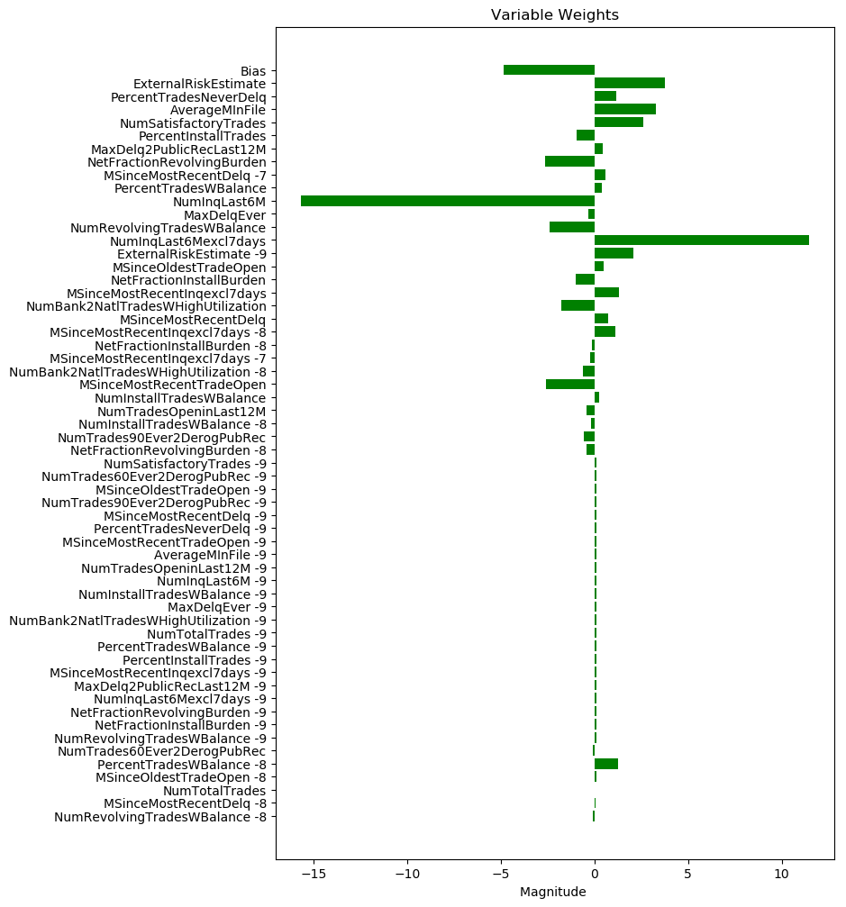
Figure 1. A visualisation of the weights learnt by logistic regression on the FICO dataset. Weights are ordered by their median contribution to the score of each datapoint over the entire dataset, with a positive sign indicating that they drive the classifier towards a score of “good”.

6. Conclusion

This is the first work to show how coherent counterfactual explanations can be generated for the mixed datasets commonly used in the real world, and the first to propose a concrete method for generating diverse counterfactuals. As such the methods proposed in this paper provide an significant step forward in what can be done with counterfactual explanations. Generalising the approach to non-linear functions, and indeed to non-differentiable classifiers such as k-nearest neighbour or random forests, looks to be a useful direction for future work. However, linear functions represent part of machine learning that “just works” and are consistently used by industry and data scientists in a wide range of scenarios. Reliable methods such as those discussed for generating both coherent and diverse explanations are needed if we want people to make use of them.

Collaboration between policy and technology is a two-way street. Just as policy must respect the limitations of technology in what it calls for, it is important to build the supporting technology in response to policy proposals. Compelling ideas such as counterfactual explanations are of little use unless we develop the technology to make them work. This paper has addressed major technological issues in one of the most substantial use cases for counterfactual explanations namely linear models for mixed financial data. As mentioned in section 5.2, the brute force enumeration of previous approaches do not scale to these datasets. Our work represents progress towards making methods for counterfactual explanation that “just work ” out of the box. Full source code can be found at https://bitbucket.org/ChrisRussell/diverse-coherent-explanations/.

References

- (1)
- Binns et al. (2018) Reuben Binns, Max Van Kleek, Michael Veale, Ulrik Lyngs, Jun Zhao, and Nigel Shadbolt. 2018. ‘It’s Reducing a Human Being to a Percentage’: Perceptions of Justice in Algorithmic Decisions. In Proceedings of the 2018 CHI Conference on Human Factors in Computing Systems. ACM, 377.
- Buchanan and Shortliffe (1984) B.G. Buchanan and E.H. Shortliffe. 1984. Rule Based Expert Systems: The MYCIN Experiments of the Stanford Heuristic Programming Project. Addison-Wesley, Chapter 18.
- Caruana et al. (1999) R. Caruana, H. Kangarloo, J. D. Dionisio, U. Sinha, and D. Johnson. 1999. Case-based explanation of non-case-based learning methods. Proceedings of the AMIA Symposium (1999), 212–215. PMID: 10566351 PMCID: PMC2232607.
- Craven and Shavlik (1996) Mark Craven and Jude W. Shavlik. 1996. Extracting tree-structured representations of trained networks. Advances in neural information processing systems, 24–30. http://papers.nips.cc/paper/1152-extracting-tree-structured-representations-of-trained-networks.pdf [Online; accessed 2017-10-16].
- Doshi-Velez et al. (2017) Finale Doshi-Velez, Mason Kortz, Ryan Budish, Chris Bavitz, Sam Gershman, David O’Brien, Stuart Schieber, James Waldo, David Weinberger, and Alexandra Wood. 2017. Accountability of AI under the law: The role of explanation. arXiv preprint arXiv:1711.01134 (2017).
- Gurobi Optimization (2018) LLC Gurobi Optimization. 2018. Gurobi Optimizer Reference Manual. http://www.gurobi.com
- Kim et al. (2014) Been Kim, Cynthia Rudin, and Julie A. Shah. 2014. The bayesian case model: A generative approach for case-based reasoning and prototype classification. Advances in Neural Information Processing Systems, 1952–1960.
- Kment (2006) Boris Kment. 2006. Counterfactuals and explanation. Mind 115, 458 (2006), 261–310.
- Lewis (1973) David Lewis. 1973. Counterfactuals. Blackwell, Oxford.
- Lim and Dey (2009) Brian Y Lim and Anind K Dey. 2009. Assessing demand for intelligibility in context-aware applications. In Proceedings of the 11th international conference on Ubiquitous computing. ACM, 195–204.
- Lipton (2016) Zachary C. Lipton. 2016. The Mythos of Model Interpretability. arXiv:1606.03490 [cs, stat] (10 6 2016). http://arxiv.org/abs/1606.03490 arXiv: 1606.03490.
- Lundberg and Lee (2017) Scott Lundberg and Su-In Lee. 2017. A Unified Approach to Interpreting Model Predictions. arXiv:1705.07874 [cs, stat] (22 5 2017). http://arxiv.org/abs/1705.07874 arXiv: 1705.07874.
- Martens et al. (2007) David Martens, Bart Baesens, Tony Van Gestel, and Jan Vanthienen. 2007. Comprehensible credit scoring models using rule extraction from support vector machines. European journal of operational research 183, 3 (2007), 1466–1476.