IPPP/19/4

Modelling and tuning in top quark physics

Marek Schönherr

Theoretical Physics Department, CERN, CH-1211 Geneva 23, Switzerland
and

Institute for Particle Physics Phenomenology, Department of Physics, Durham University, Durham, DH1 3LE, UK

In this proceedings I discuss the general strategy and impact of tuning Monte-Carlo event generators for physics processes involving top quarks. Special emphasis is put on disinguishing the different usages of event generators in the experiments and the subsequent implications on the tuning process. The current status of determining tune uncertainties is also discussed.

PRESENTED AT

$11^{\mathrm{th}}$ International Workshop on Top Quark Physics
Bad Neuenahr, Germany, September 16–21, 2018

1 Introduction

Monte-Carlo event generators [1, 2, 3, 4] are generally used in (at least) two fundamentally different ways:

• They are used to calculate theory predictions. Here, parameters in the perturbative regime are dictated by first principles or theory biases. Parameters of models for non-perturbative physics are determined universally in well-defined and limited sets of observables (akin to PDF determinations).

• They are used for data modelling. To this end, all available parameters are tuned to best reproduce the measured data of a specific process or in a specific observable. The resulting distributions lose all predictivity, but are very useful to determine acceptances, efficiencies, systematic correlations, etc.

Both cases are valid and needed, but must be clearly distinguished. This is especially relevant in the context of tuning the parameters of the models for non-perturbative physics employed by modern Monte-Carlo event generators.

This distinction becomes more relevant the smaller the target uncertainty of the prediction and the measurement become, and thus gains prominence in current and future cutting edge measurements in the top quark sector. In this presentation, I highlight the standard paradigms of tuning Monte-Carlo event generators and will comment on how the uncertainty of these tunes can be assessed.

2 Tuning strategies

Monte-Carlo event generators are built by factorising collisions into different stages with different characteristic energy regimes, e.g. proton fragmentation, parton evolution, hard scattering, multiple interactions, hadronisation, hadron decays, etc, cf. Tab. 1. This factorisation also means that each stage is independent of the details of the other stages. For example, the hadronisation only depends on the colours, flavours and momenta of the parton ensemble at relatively small separations of $\mathcal{O}(\Lambda_{\text{QCD}})$. Each stage is then tuned individually as much as possible: Hadron decay parameters are first fitted to decay data from $b$-/$c$-factories. Then, the hadronisation parameters are tuned to $e^{+}e^{-}$ data at various energies ($b$-factories, SLD, LEP), before the parameters of the multiple interaction model, beam remnant parametrisation, etc. are tuned to hadron collider data. In all stages RIVET [5] and PROFESSOR [6] are the commonly used tools.

	HERWIG 7	PYTHIA 8	SHERPA $\int_{A}^{B}$
PS	$\tilde{q}$-Shower	Default Parton Shower	CSSHOWER $\int_{A}^{B}$
	Dipole Shower	DIRE	DIRE $\int_{A}^{B}$
		VINCIA
MI	soft gluon model	sophisticated	old PYTHIA-style $\int_{A}^{B}$
	& hard scat. model	interleaved model	non-interleaved $\int_{A}^{B}$
	(Jimmy-based)
Had	Cluster	Lund String	Mod. Cluster $\int_{A}^{B}$
	Interface to		Interface to $\int_{A}^{B}$
	Lund String		Lund String $\int_{A}^{B}$
MB	MinBias	MinBias	– $\int_{A}^{B}$

Table 1: List of parton showers and non-perturbative models employed by multi-purpose event generators.

Tuning the non-perturbative models of an event generator generally bases on the minimisation of the following definition of $\chi^{2}$ dependent on a set of parameters $\vec{\mathbf{x}}$

$$\chi^{2}(\vec{\mathbf{x}})=\frac{1}{N}\sum\limits_{i\in\mathcal{O}}w_{i}\,\frac{\left(\text{MC}_{i}(\vec{\mathbf{x}})-\text{Data}_{i}\right)^{2}}{\sigma_{i,\text{Data}}^{2}}\;,$$ (1)

wherein $N$ is the number of observables the index $i$ runs over, $\text{MC}_{i}(\vec{\mathbf{x}})$ is the Monte Carlo prediction given the parameter set $\vec{\mathbf{x}}$, $\text{Data}_{i}$ is the measured data and $\sigma_{i,\text{Data}}$ is its uncertainty [6, 7].

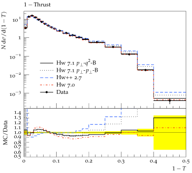
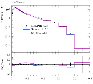
Figure 1: Example of the quality of tuning of different releases of the HERWIG (left) and SHERPA (right) generators compared to data taken by the DELPHI coll. [8].

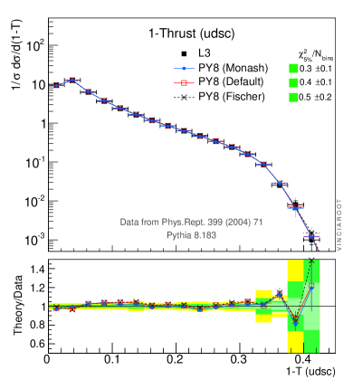
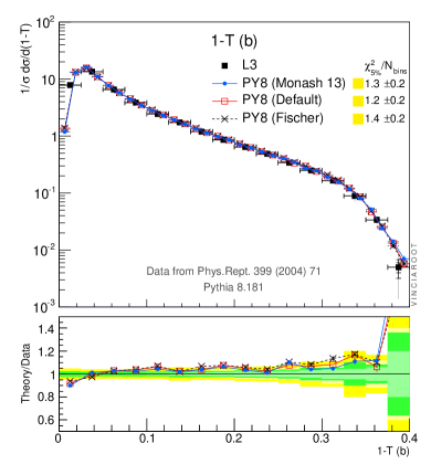
Figure 2: Example of the quality of tuning in PYTHIA 8 for light (left) and $b$ jets (right) compared to data taken by the L3 collaboration [9]. Figures taken from [7].

As the standard setups used to tune the non-perturbative models only include limited perturbative information, caution must be applied when including observables that receive sizeable contributions from multijet final state. They, thus, can only be included if the physics that should be modelled perturbatively is included properly before engaging the non-perturbative event phases. [10]

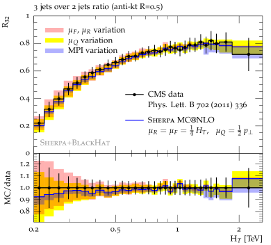
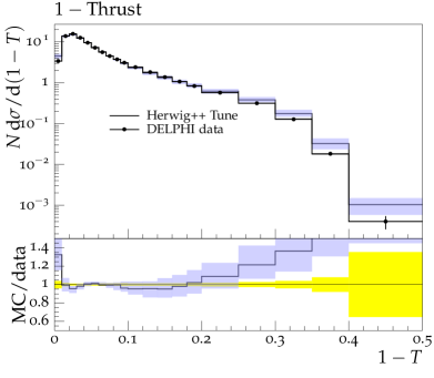
Figure 3: Example of tune uncertainties defined through “reasonable” variations of selected model parameters (left, for the $R_{32}$ at the LHC) and systematically defined Eigentunes (right, for $1-T$ at LEP). Left figure taken from [11].

Traditionally, expert-defined variations of certain key parameters within “reasonable” ranges are used as simple stand-ins to gauge the uncertainty of the given tune, i.e. minimum point $\vec{\mathbf{x}}$ of the $\chi^{2}(\vec{\mathbf{x}})$ distribution. Therein, the “reasonable” range is usually defined such that the resulting uncertainty is comparable to the data uncertainty in the measurement [12]. This can be improved by assuming that the test statistics were distributed according to a second order polynomial around the above minimum or optimal tune. A variation around this minimum to some $\Delta\chi^{2}$ then forms an ellipsoid with $2\,\text{dim}(\vec{\mathbf{x}})$ principal vectors forming the eigenvectors of the covariance matrix computed around the minimum. Variations with the customary $\Delta\chi^{2}=1$, defining a $1\,\sigma$ variation under the above assumption, however, lead to empirically too small variations. Thus, a more useful value of $\Delta\chi^{2}=\tfrac{1}{2}\,\text{dim}(\vec{\mathbf{x}})$ is adopted in practise [13]. Future approaches, relaxing the above assumptions of the behaviour of the models around the minimum, are currently being developed and will lead to more agnostic definitions of tuning uncertainties, necessitating less arbitrary definitions of “reasonableness”.

3 Influence on top quark observables

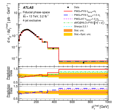
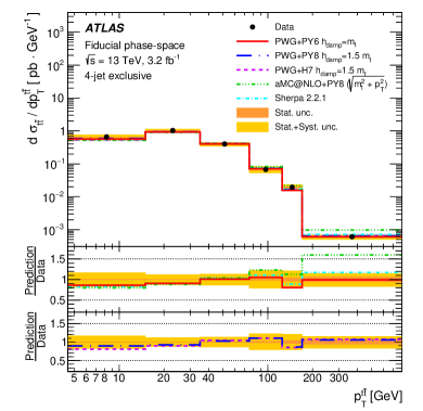
Figure 4: General $t\overline{t}$ observables show only very little dependence on the details of the non-perturbative models and are well described by current tunes. Figures taken from [14].

In contrary to most data used in tuning Monte-Carlo event generators, top quark processes are unique in that they always involve $b$-quarks and almost always involve gluons. Both are not as constrained as their light quark counter parts.

Most observables in standard $t\overline{t}$ measurements show only very little dependence on the details of the non-perturbative modelling. Subsequently, the uncertainty of the current global tunes of all modern event generators hardly impact these measurements. Nonetheless, dedicated examples can be found where they impact. To reduce the tuning uncertainty on this class of observables, one may be tempted to include top quark observables in the tunes. This would, however, exclude exactly these observables from collection of observables unbiased theoretical predictions can be made for. A different approach would be to find suitable proxies to better constrain the gluon and bottom related parameters of the non-perturbative models. Such measurements are already on their way ($\Delta R(B,B)$ at the LHC [15, 16] for $t\overline{t}b\overline{b}$ observables, gluon jet data at LEP [17, 18] and LHC for gluon jet fragmentation, etc.), but will need to be more routinely used in global tuning efforts.

Not all cases of mismodelling are related to imperfect tuning or missing aspects in the non-perturbative models though. The transverse momentum distribution of the top quark in $t\overline{t}$production can be resolved by including electroweak corrections, at least in the large transverse momentum region, as shown in [21].

4 Conclusions

It is important to clearly distinguish (at least) two types of Monte-Carlo event generator usage: calculating theory predictions and providing a controllable and fast tool for data reproduction. While both use cases are perfectly valid in their own right, they mandate different treatments of the tuning of the parameters of their models of non-perturbative physics. If the Monte-Carlo event generator is used to best reproduce already measured data, e.g. for statistical analysis or the evaluation of internal correlations, all parameters of the non-perturbative physics models (and some of the perturbative calculation) may be adjusted to best fit the data of that measurement. Of course, by definition, the resulting output of the Monte-Carlo event generator is no theoretical prediction in this case but fulfils its role as multidimensional fit function. If, on the other hand, a theoretical prediction is sought, the parameters of the non-perturbative models must be tuned to a well-defined and limited global set of observables, while those of the perturbative calculation should be set to a theoretically defined value. The resulting tunes aim to describe all available data to the best ability of the employed models are can be used for theory predictions for all observables except the input observables.

Currently, no tune provided by the authors of the used Monte-Carlo event generators makes use of any direct top quark data. Thus, these tunes can be employed for theory predictions for top quark observables. Of course, when observables receive a non-negligible non-perturbative contribution, mismodelling may happen as the employed models are phenomenological in nature and do not directly derive from first principles and can, thus, not fully capture the underlying dynamics. Conversely, mismodelling does not necessarily originate in suboptimal tuning or incomplete models and the impact of improved perturbative inputs should not be underestimated.

Uncertainties on existing tunes can currently only be assessed using some level of arbitrary “reasonableness” criterion, either through a hand-picked set of representative variations or a set of Eigentunes where the magnitude of the $1\,\sigma$ ellipsoid is set manually. New methods along the lines of using data replica to define alternative tunes are currently being explored.

ACKNOWLEDGEMENTS

MS acknowledges the support of the Royal Society through the award of a University Research Fellowship.

References

- [1] A. Buckley et al., Phys. Rept. 504, 145 (2011) doi:10.1016/j.physrep.2011.03.005 [arXiv:1101.2599 [hep-ph]].
- [2] T. Sjöstrand et al., Comput. Phys. Commun. 191, 159 (2015) doi:10.1016/j.cpc.2015.01.024 [arXiv:1410.3012 [hep-ph]].
- [3] J. Bellm et al., Eur. Phys. J. C 76, no. 4, 196 (2016) doi:10.1140/epjc/s10052-016-4018-8 [arXiv:1512.01178 [hep-ph]].
- [4] T. Gleisberg, S. Höche, F. Krauss, M. Schönherr, S. Schumann, F. Siegert and J. Winter, JHEP 0902, 007 (2009) doi:10.1088/1126-6708/2009/02/007 [arXiv:0811.4622 [hep-ph]].
- [5] A. Buckley, J. Butterworth, L. Lönnblad, D. Grellscheid, H. Hoeth, J. Monk, H. Schulz and F. Siegert, Comput. Phys. Commun. 184, 2803 (2013) doi:10.1016/j.cpc.2013.05.021 [arXiv:1003.0694 [hep-ph]].
- [6] A. Buckley, H. Hoeth, H. Lacker, H. Schulz and J. E. von Seggern, Eur. Phys. J. C 65, 331 (2010) doi:10.1140/epjc/s10052-009-1196-7 [arXiv:0907.2973 [hep-ph]].
- [7] P. Skands, S. Carrazza and J. Rojo, Eur. Phys. J. C 74, no. 8, 3024 (2014) doi:10.1140/epjc/s10052-014-3024-y [arXiv:1404.5630 [hep-ph]].
- [8] P. Abreu et al. [DELPHI Collaboration], Z. Phys. C 73, 11 (1996). doi:10.1007/s002880050295
- [9] P. Achard et al. [L3 Collaboration], Phys. Rept. 399, 71 (2004) doi:10.1016/j.physrep.2004.07.002 [hep-ex/0406049].
- [10] M. Aaboud et al. [ATLAS Collaboration], ATL-PHYS-PUB-2013-017
- [11] S. Höche and M. Schönherr, Phys. Rev. D 86, 094042 (2012) doi:10.1103/PhysRevD.86.094042 [arXiv:1208.2815 [hep-ph]].
- [12] J. Alcaraz Maestre et al. [SM and NLO MULTILEG Working Group and SM MC Working Group], arXiv:1203.6803 [hep-ph].
- [13] A. Buckley and H. Schulz, Adv. Ser. Direct. High Energy Phys. 29, 281 (2018) doi:10.1142/9789813227767_0013 [arXiv:1806.11182 [hep-ph]].
- [14] M. Aaboud et al. [ATLAS Collaboration], JHEP 1810, 159 (2018) doi:10.1007/JHEP10(2018)159 [arXiv:1802.06572 [hep-ex]].
- [15] V. Khachatryan et al. [CMS Collaboration], JHEP 1103, 136 (2011) doi:10.1007/JHEP03(2011)136 [arXiv:1102.3194 [hep-ex]].
- [16] M. Aaboud et al. [ATLAS Collaboration], arXiv:1812.09283 [hep-ex].
- [17] N. Fischer, S. Gieseke, S. Plätzer and P. Skands, Eur. Phys. J. C 74, no. 4, 2831 (2014) doi:10.1140/epjc/s10052-014-2831-5 [arXiv:1402.3186 [hep-ph]].
- [18] N. Fischer et al. [OPAL Collaboration], Eur. Phys. J. C 75, no. 12, 571 (2015) doi:10.1140/epjc/s10052-015-3766-1 [arXiv:1505.01636 [hep-ex]].
- [19] S. Höche, J. Huang, G. Luisoni, M. Schönherr and J. Winter, Phys. Rev. D 88, no. 1, 014040 (2013) doi:10.1103/PhysRevD.88.014040 [arXiv:1306.2703 [hep-ph]].
- [20] S. Höche, F. Krauss, P. Maierhöfer, S. Pozzorini, M. Schönherr and F. Siegert, Phys. Lett. B 748, 74 (2015) doi:10.1016/j.physletb.2015.06.060 [arXiv:1402.6293 [hep-ph]].
- [21] C. Gütschow, J. M. Lindert and M. Schönherr, Eur. Phys. J. C 78, no. 4, 317 (2018) doi:10.1140/epjc/s10052-018-5804-2 [arXiv:1803.00950 [hep-ph]].
- [22] E. Bothmann, F. Krauss and M. Schönherr, Eur. Phys. J. C 78, no. 3, 220 (2018) doi:10.1140/epjc/s10052-018-5696-1 [arXiv:1711.02568 [hep-ph]].