Model and Reinforcement Learning for Markov Games with Risk Preferences

Abstract

We motivate and propose a new model for non-cooperative Markov game which considers the interactions of risk-aware players. This model characterizes the time-consistent dynamic “risk” from both stochastic state transitions (inherent to the game) and randomized mixed strategies (due to all other players). An appropriate risk-aware equilibrium concept is proposed and the existence of such equilibria is demonstrated in stationary strategies by an application of Kakutani’s fixed point theorem. We further propose a simulation-based $Q$-learning type algorithm for risk-aware equilibrium computation. This algorithm works with a special form of minimax risk measures which can naturally be written as saddle-point stochastic optimization problems, and covers many widely investigated risk measures. Finally, the almost sure convergence of this simulation-based algorithm to an equilibrium is demonstrated under some mild conditions. Our numerical experiments on a two player queuing game validate the properties of our model and algorithm, and demonstrate their worth and applicability in real life competitive decision-making.

Keywords: Markov games; time-consistent risk preferences; fixed point theorem; $Q$-learning

1 Introduction

Markov games (a.k.a stochastic games) generalize Markov decision processes (MDPs) to the multi-player setting. In the classical case, each player seeks to minimize his expected costs. In a corresponding equilibrium, no player can decrease his expected costs by changing his strategy. We often want to compute equilibria to predict the outcome of the game and understand the behavior of the players.

In this paper, we directly account for the risk preferences of the players in a Markov game. Informally, risk aversion is at least weakly preferring a gamble with smaller variance when payoffs are the same. Risk-averse players give more attention to low probability but high cost events compared to risk-neutral players. Models for the risk preferences of a single agent are well established [2, 45] for the static problems and [44, 48] for the dynamic case. We extend these ideas to general sum Markov games and extend the framework of Markov risk measures [44, 48] to the multi-agent setting. Our model specifically addresses the risk from the stochastic state transitions as well as the risk from the randomized strategies of the other players. The traditional multilinear formulation approach [1, 30] for computing equilibria in robust games fails in our settings, because our model has an intrinsic bilinear term due to the product of probabilities (the state transitions and mixed strategies) which leads to computational intractability. Thus, it is necessary to develop an alternative algorithm to compute equilibria.

Risk Preferences

Expected utility theory [14, 51, 52] is a highly developed framework for modeling risk preferences. Yet, some experiments [35] show that real human behavior may violate the independence axiom of expected utility theory. Risk measures (as developed in [2, 45]) do not require the independence axiom and have favorable properties for optimization.

In the dynamic setting, [44, 48] develop the class of Markov (a.k.a. dynamic/nested/iterated) risk measures and establish their connection to time-consistency. This class of risk measures is notable for its recursive formulation, which leads to dynamic programming equations. Practical computational schemes for solving large-scale risk-aware MDPs have been proposed, for instance, $Q$-learning type algorithms [25, 26, 27] and simulation-based fitted value iteration [55].

Risk-sensitive/Robust Games

Risk-sensitive games have already been considered in [3, 5, 19, 28, 32]. Risk-sensitivity refers to the specific certainty equivalent $\left(1/\theta\right)\ln\left(\mathbb{E}\left[\exp\left(\theta\,X\right)\right]\right)$ where $\theta>0$ is the risk sensitivity parameter. [3, 19] focus on zero-sum risk-sensitive games under continuous time setting.

Robust games study ambiguity about costs and/or state transition probabilities of the game. [1] develop the robust equilibrium concept where each player optimizes against the worst-case expected cost over the range of model ambiguity. This paradigm is extended to Markov games in [30], and the existence of robust Markov perfect equilibria is demonstrated. [1, 30] formulate robust Markov perfect equilibria as multilinear systems.

Games with risk preferences are not artificial; rather, they emerge organically from many real problems. Traffic equilibrium problems with risk-averse agents are analyzed in [6] with non-cooperative game theory. The preferences of risk-aware adversaries are modeled in Stackelberg security games in [43], and a computational scheme for robust defender strategies is presented.

Contributions of This Work

We make three main contributions in this paper:

1. We develop a model for risk-aware Markov games where agents have time-consistent risk preferences. This model specifically addresses both sources of risk in a Markov game: (i) the risk from the stochastic state transitions and (ii) the risk from the randomized strategies of the other players.

2. We propose a notion of ‘risk-aware’ Markov perfect equilibria for this game. We show that there exist risk-aware equilibria in stationary strategies.

3. We create a practical simulation-based $Q$-learning type algorithm for computing risk-aware Markov perfect equilibria, and we show that it converges to an equilibrium almost surely. This algorithm is model-free and so does not require any knowledge of the true model, and thus can search for equilibria purely by observations.

2 Risk-aware Markov Games

In this section, we develop risk-aware Markov games. Our game consists of the following ingredients: finite set of players $\mathcal{I}$; finite set of states $\mathcal{S}$; finite set of actions $\mathcal{A}^{i}$ for each player $i\in\mathcal{I}$; strategy profiles $\mathcal{A}:=\times_{i\in\mathcal{I}}\mathcal{A}^{i}$; state-action pairs $\mathcal{K}:=\mathcal{S}\times\mathcal{A}$; transition kernel $P(\cdot|s,\,a)\in\mathcal{P}(\mathcal{S})$ (here $\mathcal{P}(\mathcal{S})$ denotes the distribution over $\mathcal{S}$) for all $(s,\,a)\in\mathcal{K}$, and cost functions $c^{i}:\mathcal{S}\times\mathcal{A}\rightarrow\mathbb{R}$ for all players $i\in\mathcal{I}$.

Each round $t\geq 0$ of the game has four steps: (i) first, all players observe the current state $s_{t}\in\mathcal{S}$; (ii) second, each player $i\in\mathcal{I}$ chooses $a_{t}^{i}\in\mathcal{A}^{i}$ (all moves are simultaneous and independent, and the corresponding strategy profile is $a_{t}=\left(a_{t}^{i}\right)_{i\in\mathcal{I}}$); (iii) third, each player $i\in\mathcal{I}$ realizes cost $c^{i}\left(s_{t},\,a_{t}\right)$; and (iv) lastly, the state transitions to $s_{t+1}$ according to $P\left(\cdot\,|\,s_{t},\,a_{t}\right)$.

We next characterize the players’ strategies. In this work, we focus on ‘stationary strategies’. Stationary strategies prescribe a player the same probabilities over his actions each time the player visits a certain state, no matter what route he follows to reach that state. Stationary strategies are more prevalent than normal strategies (which rely on the entire history), due to their mathematical tractability [53, 17, 30]. Furthermore, the memoryless property of stationary strategies conforms to real human behavior [53].

We introduce some additional notations to characterize stationary strategies $x$. Let $\mathcal{P}(\mathcal{A}^{i})$ denote the distribution over $\mathcal{A}^{i}$. For each player $i\in\mathcal{I}$ and state $s\in\mathcal{S}$, $x_{s}^{i}\in\mathcal{P}\left(\mathcal{A}^{i}\right)$ is the mixed strategy over actions where $x_{s}^{i}\left(a^{i}\right)$ denotes the probability of choosing $a^{i}$ at state $s$. We define the strategy $x^{i}:=(x_{s}^{i})_{s\in\mathcal{S}}\in\mathcal{X}^{i}:=\times_{s\in\mathcal{S}}\mathcal{P}\left(\mathcal{A}^{i}\right)$ of player $i$, the multi-strategy $x:=\left(x^{i}\right)_{i\in\mathcal{I}}\in\mathcal{X}:=\times_{i\in\mathcal{I}}\mathcal{X}^{i}$ of all players, the complementary strategy $x^{-i}:=(x^{j})_{j\neq i}\in\mathcal{X}^{-i}:=\times_{j\neq i}\mathcal{X}^{j}$, and the multi-strategy $x_{s}=\left(x_{s}^{i}\right)_{i\in\mathcal{I}}\in\mathcal{X}_{s}:=\times_{i\in\mathcal{I}}\mathcal{P}\left(\mathcal{A}^{i}\right)$ for all players in state $s\in\mathcal{S}$. We sometimes write a multi-strategy as $x=(u^{i},\,x^{-i})$ to emphasize player $i$’s strategy $u^{i}$.

There are two sources of stochasticity in the cost sequence: the stochastic state transitions characterized by the transition kernel $P(\cdot|s,\,a)$, and the randomized mixed strategies of players characterized by $x^{-i}$. In this work, we consider the risk from both sources of stochasticity. We begin by constructing the framework for evaluating the risk of sequences of random variables. A dynamic risk measure is a sequence of conditional risk measures each mapping a future stream of random costs into a risk assessment at the current stage, following the definition of risk maps from [48], and satisfying the stationary and time-consistency property of [44, Definition 3] and [47, Definition 1]. We assume each conditional risk measure satisfies three axioms: normalization, convexity, and positive homogeneity , which were originally introduced for static risk measures in the pioneering paper [2]. Here “convexity” characterizes the risk-averse behavior of players. From [47, Definition 1], a risk-aware optimal policy is time-consistent if, the risk of the sub-sequence of random outcome from any future stage is optimized by the resolved policy. In the Appendix, we give explicit definitions of the above three axioms of risk measures, stationary and time-consistency risk preferences, and derivation of recursive evaluation of dynamic risk.

From [44, Theorem 4] and [47, Proposition 4], time-consistency allows for a recursive (iterative) evaluation of risk. The infinite-horizon discounted risk for player $i$ under multi-strategy $x$ will be:

$$J_{s_{0}}^{i}(x^{i},\,x^{-i}):= \rho^{i}(c^{i}(s_{0},\,a_{0})+\gamma\,\rho^{i}(c^{i}(s_{1},\,a_{1})$$

$$+\gamma\,\rho^{i}\left(c^{i}(s_{2},\,a_{2})+\cdot\cdot\cdot\right))),$$ (1)

where $\rho^{i}$ is a one-step conditional risk measure that maps random cost from the next stage to current stage, with respect to the joint distribution of randomized mixed strategies and transition kernel. In Eq. (19), each $c^{i}(s_{t},\,a_{t}),\,t\geq 1$ is governed by the joint distribution of randomized mixed strategies and transition kernel

$$\times_{i\in\mathcal{I}}x_{s_{t}}^{i}(a_{t}^{i})P(s_{t}|s_{t-1},\,a_{t-1}),$$

which is defined for fixed $(s_{t-1},\,a_{t-1})$ and for all $s_{t}$ and $a_{t}^{i}$. The initial cost $c^{i}(s_{0},\,a_{0})$ is only governed by the random mixed strategies distribution $\times_{i\in\mathcal{I}}x^{i}_{s_{0}}(a_{0}^{i})$.

The corresponding best response function for player $i$ is:

$$\min_{x^{i}\in\mathcal{X}^{i}}\,J_{s_{0}}^{i}(x^{i},\,x^{-i}).$$ (2)

Suppose we replace all $\rho^{i}$ with expectation $\mathbb{E}$ in Eq. (19) which leads to $\mathbb{E}_{s}^{x}\left[\sum_{t=0}^{\infty}\gamma^{t}c^{i}\left(s_{t},\,a_{t}\right)\right]$, where $\mathbb{E}_{s}^{x}$ denotes expectation with respect to multi-strategies $x$, then Problem (2) will become risk-neutral. Thus our formulation recovers the risk-neutral game as a special case.

Denote the ingredients of game $\left\{J_{s}^{i}(x^{i},\,x^{-i})\right\}_{s\in\mathcal{S},\,i\in\mathcal{I}}$ as $\left\{\mathcal{I},\,\mathcal{S},\,\mathcal{A},\,P,\,c,\,\rho\right\}$. In line with the classical definition of Markov perfect equilibrium in [17], we now define risk-aware Markov perfect equilibrium.

Definition 1.

(Risk-aware Markov perfect equilibrium) A multi-strategy $x\in\mathcal{X}$ is a risk-aware Markov perfect equilibrium for $\left\{\mathcal{I},\,\mathcal{S},\,\mathcal{A},\,P,\,c,\,\rho\right\}$ if

$$J_{s}^{i}(x^{i},\,x^{-i})\leq J_{s}^{i}(u^{i},\,x^{-i}),\,\forall s\in\mathcal{S},\,u^{i}\in\mathcal{X}^{i},\,i\in\mathcal{I}.$$ (3)

In Definition 1, each player $i\in\mathcal{I}$ implements a (risk-aware) stationary best response given the stationary complementary strategy $x^{-i}$. It also states that $x$ is an equilibrium if and only if no player can reduce his discounted risk by unilaterally changing his strategy.

Existence of Stationary Equilibria

We prove the existence of stationary equilibira in this section. Let $v^{i}$ denote player $i$’s value function, which is an estimate of the discounted risk starting from the next state $S^{\prime}$. For each player $i$, the value of the stationary strategy $x\in\mathcal{X}$ in state $s\in\mathcal{S}$ is defined to be $v^{i}\left(s\right):=J_{s}^{i}(x)$, and $v^{i}:=\left(v^{i}\left(s\right)\right)_{s\in\mathcal{S}}$ is the entire value function for player $i$. The space of value functions for all players is $\mathcal{V}:=\times_{i\in\mathcal{I}}\mathbb{R}^{|\mathcal{S}|}$, equipped with the supremum norm $\|v\|_{\infty}:=\max_{s\in\mathcal{S},\,i\in\mathcal{I}}|v^{i}\left(s\right)|$. Eq. (19) states that each player must evaluate the stage-wise risk of random variables on $\mathcal{A}\times\mathcal{S}$, formulated as

$$c^{i}\left(s,\,A\right)+\gamma\,v^{i}\left(S^{\prime}\right),$$ (4)

where $A$ is the random strategy profile chosen from $\mathcal{A}$ according to $x_{s}$, and $S^{\prime}$ is the random next state visited (which first depends on $x$ through the random choice of strategy profile $a$, and then depends on the transition kernel $P\left(\cdot\,|\,s,\,a\right)$ after $a\in\mathcal{A}$ is realized).

Recall that in state $s\in\mathcal{S}$, the probability that $a=(a^{i})_{i\in\mathcal{I}}\in\mathcal{A}$ is chosen and then the system transitions to state $k\in\mathcal{S}$ is $\left(\times_{i\in\mathcal{I}}x_{s}^{i}\left(a^{i}\right)\right)P(k\,|\,s,\,a)$. The probability distribution of the strategy profile $a\in\mathcal{A}$ and next state visited $k\in\mathcal{S}$ is given by the matrix

$$P_{s}\left(u_{s}^{i},\,x_{s}^{-i}\right)$$

$$:= \left[u_{s}^{i}\left(a^{i}\right)\left(\times_{j\neq i}x_{s}^{j}\left(a^{j}\right)\right)P(k\,|\,s,\,a)\right]_{\left(a,\,k\right)\in\mathcal{A}\times\mathcal{S}},$$ (5)

where we explicitly denote the dependence on the multi-strategy $x_{s}=\left(u_{s}^{i},\,x_{s}^{-i}\right)$ in state $s$. For simplicity, we often write $P_{s}$ instead of $P_{s}\left(u_{s}^{i},\,x_{s}^{-i}\right)$ when it is not necessary to indicate the dependence on $(u,x)$.

Let $C_{s}^{i}\left(v^{i}\right):=\left(c^{i}\left(s,\,A\right)+\gamma\,v^{i}\left(S^{\prime}\right)\right)$ be the random cost-to-go for player $i$ at state $s$. Based on the Fenchel-Moreau representation of risk [18, 45, 20], the convex risk of random cost-to-go denoted by $\psi_{s}^{i}(u_{s}^{i},\,x_{s}^{-i},\,v^{i})$ can be computed as the worst-case expected cost-to-go

$$\psi_{s}^{i}(u_{s}^{i},\,x_{s}^{-i},\,v^{i}):= \rho^{i}\left(c^{i}(s\,,A)+\gamma\,v^{i}\left(S^{\prime}\right)\right)$$

$$= \sup_{\mu\in\mathcal{M}_{s}^{i}(P_{s})}\left\{\langle\mu,\,C_{s}^{i}\left(v^{i}\right)\rangle-b_{s}^{i}(\mu)\right\},$$

where $\left\{\mathcal{M}_{s}^{i}(P_{s})\right\}_{s\in\mathcal{S},\,i\in\mathcal{I}}\subset\mathcal{P}(\mathcal{A}\times\mathcal{S})$ is the risk envelope of $\rho^{i}$ that depends on the distribution $P_{s}$, and $\left\{b_{s}^{i}\right\}_{s\in\mathcal{S},\,i\in\mathcal{I}}\text{ : }\mathcal{P}\left(\mathcal{A}\times\mathcal{S}\right)\rightarrow\mathbb{R}$ are convex functions satisfying $\inf_{\mu\in\mathcal{P}(\mathcal{A}\times\mathcal{S})}b_{s}^{i}(\mu)=0$ for all $i\in\mathcal{I}$ and $s\in\mathcal{S}$. To connect to risk-neutral games, we can just choose all $\mathcal{M}_{s}^{i}(P_{s})$ to be singletons $\{P_{s}\left(u_{s}^{i},\,x_{s}^{-i}\right)\}$ and $b_{s}^{i}(\mu)=0$ for all $\mu\in\mathcal{M}_{s}^{i}(P_{s})$, $i\in\mathcal{I}$, and $s\in\mathcal{S}$.

We next introduce further assumptions on $\rho^{i}$, $\left\{\mathcal{M}_{s}^{i}(P_{s})\right\}_{s\in\mathcal{S},\,i\in\mathcal{I}}$, and $\left\{b_{s}^{i}\right\}_{s\in\mathcal{S},\,i\in\mathcal{I}}$, that will lead to the existence of stationary equilibria.

Assumption 1.

(i) All $\rho^{i}$ are law invariant, $\rho^{i}(X)=\rho^{i}(Y)$ for all $X=_{D}Y$, where $=_{D}$ denotes equality in distribution.

(ii) $\left\{\mathcal{M}_{s}^{i}(P_{s})\right\}_{s\in\mathcal{S},\,i\in\mathcal{I}}\subset\mathcal{P}\left(\mathcal{A}\times\mathcal{S}\right)$ is a collection of set-valued mappings where $\mathcal{M}_{s}^{i}(P_{s})$ are closed and polyhedral convex for all $P_{s}$. Explicitly, there exists $M\geq 1$ linear constraints and $[M]:=\{1,2,...,M\}$. Then $\mathcal{M}_{s}^{i}(P_{s})$ is defined as:

$$\left\{\mu\in\mathbb{R}^{|\mathcal{A}||\mathcal{S}|}:\begin{array}[]{cc}A_{s,\,m}^{i}\,\mu+f_{m}(P_{s})\geq h_{s,\,m}^{i},m\in[M],\\ e^{T}\mu=1,\\ \mu\geq 0,\end{array}\right\}$$ (9)

where $A_{s,\,m}^{i}$ are matrices, $f_{m}$ are linear functions in $P_{s}$ and $h_{s,\,m}^{i}$ are constants.

(iii) All $\left\{b_{s}^{i}\right\}_{s\in\mathcal{S},\,i\in\mathcal{I}}$ are convex and Lipschitz continuous.

Formulation (9) explains how $\mathcal{M}_{s}^{i}(P_{s})$ depends on $P_{s}$. In addition, if $f_{m}$ depends linearly on $P_{s}$, then $f_{m}$ also depends linearly on $u_{s}^{i}$ and $x_{s}^{-i}$ by definition of $P_{s}$ in Eq. (5). In computational terms, this assumption is close to [30] which assumes polyhedral uncertainty sets for the transition probabilities in its robust Markov game model. This assumption also corresponds to the one in [16] about representation of agent risk preferences.

Example 1.

Conditional value-at-risk (CVaR) is a widely investigated coherent risk measure that computes the conditional expectation of random losses exceeding a threshold with probability $\alpha$.

CVaR can be constructed from system (9) when we choose $M=1$, $A_{s,m}^{i}=-e$, $f_{m}(P_{s})=P_{s}/(1-\alpha^{i})$, and $h_{s,m}^{i}=0$ with $m=1$.

The best response function $v_{\ast}$ corresponding to a risk-aware Markov perfect equilibrium, for all $s\in\mathcal{S},\,i\in\mathcal{I}$, satisfies

$$v_{\ast}^{i}\left(s\right)=\, \min_{u_{s}^{i}\in\mathcal{P}\left(\mathcal{A}^{i}\right)}\,J_{s}^{i}(u^{i},\,x^{-i})$$

$$=\, \min_{u_{s}^{i}\in\mathcal{P}\left(\mathcal{A}^{i}\right)}\,\psi_{s}^{i}(u_{s}^{i},\,x_{s}^{-i},\,v_{\ast}^{i}),$$ (10)

$$x_{s}^{i}\in\, \arg\min_{u^{i}\in\mathcal{X}^{i}}\,J_{s}^{i}(u^{i},\,x^{-i}),$$ (11)

and $v^{i}_{\ast}$ may not be unique. In the mapping $C_{s}^{i}\left(v^{i}\right)$ on $\mathcal{A}\times\mathcal{S}$, the players control the distribution on $\mathcal{P}\left(\mathcal{A}\times\mathcal{S}\right)$ through their mixed strategies. Eqs. (2) - (11) together simply restate Eq. (3). However, Eqs. (2) - (11) give a computational recipe that can be encoded into an operator on multi-strategies. We define this operator $\Phi$ on $\mathcal{X}$:

$$\Phi(x):=\,\Big{\{}\tilde{q}\in\mathcal{X}:\,\tilde{q}_{s}^{i}\in\arg\min_{u_{s}^{i}\in\mathcal{P}(\mathcal{A}^{i})}\psi_{s}^{i}(u_{s}^{i},\,x_{s}^{-i},\,v_{\ast}^{i}),$$

$$v_{\ast}^{i}\left(s\right)=\min_{u_{s}^{i}\in\mathcal{P}\left(\mathcal{A}^{i}\right)}\psi_{s}^{i}(u_{s}^{i},\,x_{s}^{-i},\,v_{\ast}^{i}),\,\forall s\in\mathcal{S},\,i\in\mathcal{I}\Big{\}}.$$ (12)

This operator returns the set of strategies for every player that are best responses to all other players’ strategies.

The following Theorem 1 briefly describes the existence of stationary strategies with detailed proof in the Appendix.

Theorem 1.

Suppose Assumption 1 holds, then the game $\left\{\mathcal{I},\,\mathcal{S},\,\mathcal{A},\,P,\,c,\,\rho\right\}$ has an equilibrium in stationary strategies.

Proof.

(Proof sketch) Our proof of existence of risk-aware Markov perfect equilibrium draws from [17, 30]. The main idea is to show that $\Phi$ is a nonempty, closed, and convex subset of $\mathcal{X}$, and that $\Phi$ is upper semicontinuous. Then, we apply Kakutani’s fixed point theorem to show that this correspondence $\Phi$ has a fixed point which coincides with a risk-aware Markov perfect equilibrium. ∎

3 A $Q$-Learning Algorithm

We propose a simulation-based and asynchronous algorithm for computing equilibria of the risk-aware game $\left\{\mathcal{I},\,\mathcal{S},\,\mathcal{A},\,P,\,c,\,\rho\right\}$, called Risk-aware Nash $Q$-learning (RaNashQL). This algorithm does not require a model for the cost functions $\left\{c^{i}\right\}_{i\in\mathcal{I}}$ or the transition kernel $P$, nor does not it require prior knowledge on $\mathcal{S}$. The algorithm has an outer-inner loop structure, where the risk estimation is performed in the inner loop and the equilibrium estimation is performed in the outer loop.

In each iteration of RaQL, a collection of $Q$-values for each player for all strategy profiles, is generated. The one-shot game formed by the collection of $Q$-values is called a stage game. We will later formulate stage game explicitly. The outer-inner loop structure follows [25, 27, 26] where multiple “stochastic approximation instances” for both risk estimation and $Q$-value updates are “pasted” together. We show that the Nash equilibria mapping for stage games is non-expansive, and both the risk estimation error and equilibrium estimation error are bounded by the gap between the estimated $Q$-value and the $Q$-value under the equilibrium. These two conditions allow us to prove the convergence of the algorithm using the theory of stochastic approximation, as shown in [15].

For this section, we assume that our risk measures $\left\{\rho^{i}\right\}$ have a special form as stochastic saddle-point problems to facilitate computation. Define a probability space $(\Omega,\mathcal{F},P)$ and the space of essentially bounded random variables $\mathcal{L}=L_{\infty}(\Omega,\mathcal{F},P)$.

Assumption 2.

(Stochastic saddle-point problem) For all $i\in\mathcal{I}$,

$$\rho^{i}(X)=\min_{y\in\mathcal{Y}^{i}}\max_{z\in\mathcal{Z}^{i}}\mathbb{E}_{P}\left[G^{i}(X,\,y,\,z)\right],\,\forall X\in\mathcal{L},$$ (13)

where: (i) $\mathcal{Y}^{i}\subset\mathbb{R}^{d_{1}}$ and $\mathcal{Z}^{i}\subset\mathbb{R}^{d_{2}}$ are compact and convex with diameters $D_{\mathcal{Y}}$ and $D_{\mathcal{Z}}$, respectively. (ii) $G^{i}$ is Lipschitz continuous on $\mathcal{L}\times\mathcal{Y}^{i}\times\mathcal{Z}^{i}$ with constant $K_{G}>1$. (iii) $G$ is convex in $y\in\mathcal{Y}^{i}$ and concave in $z\in\mathcal{Z}^{i}$. (iv) The subgradients of $G$ on $y$ and $z$ are Borel measurable and uniformly bounded for all $X\in\mathcal{L}$.

In [26, Theorem 3.2], conditions on $G^{i}$ are given to ensure that the corresponding minimax structure (13) is a convex risk measure. Some examples of the functions $G^{i}$ are shown in the Appendix such that the corresponding risk-aware Markov perfect equilibria exist. For instance, CVaR can be written as:

$$\textrm{CVaR}{}_{\alpha^{i}}(X):=\min_{\eta\in\mathbb{R}}\left\{\eta+\frac{1}{1-\alpha^{i}}\mathbb{E}\left[\max\left\{X-\eta,\,0\right\}\right]\right\},$$ (14)

where $\alpha^{i}\in[0,\,1)$ is the risk tolerance for player $i$.

Risk-aware Nash $Q$-learning Algorithm

RaNashQL is updated based on future equilibrium costs (which depend on all players). In contrast, single-agent $Q$-learning updates are only based on the player’s own costs. Thus, to predict equilibrium losses, every player must maintain and update a model for all other player’s costs and their risk assessments, which follows the settings in [23].

For all $\left(s,\,a\right)\in\mathcal{S}\times\mathcal{A},\,i\in\mathcal{I}$,

$$Q_{\ast}^{i}(s,\,a):= \min_{y\in\mathcal{Y}^{i}}\max_{z\in\mathcal{Z}^{i}}\mathbb{E}_{P\left(\cdot\,|\,s,\,a\right)}\big{\{}$$

$$G^{i}\left(c^{i}(s\,,A)+\gamma\,v_{\ast}^{i}(S),\,y,\,z\right)\big{\}},$$ (15)

denotes the $Q$-values corresponding to a stationary equilibrium and its best response function $v_{\ast}$. In the case of multiple equilibria, different Nash strategy profiles may have different equilibrium $Q$-values, so the pair $(v^{i}_{\ast},\,Q^{i}_{\ast})$ may not be unique.

In a multi-agent $Q$-learning algorithm, the agents play a sequence of stage games where the payoffs are the current $Q$-values. In each state $s\in\mathcal{S}$, the corresponding stage game is the collection $(Q^{i}(s))_{i\in\mathcal{I}}$, where $Q^{i}(s):=\{Q^{i}(s,\,a)\text{ : }a\in\mathcal{A}\}$ is the array of $Q$-values for player $i$ for all strategy profiles. Let $x_{s}$ be a Nash equilibrium of the stage game $(Q^{i}(s))_{i\in\mathcal{I}}$, then the corresponding Nash $Q$-value for all $i\in\mathcal{I}$ is denoted:

$$Nash^{i}(Q^{j}(s))_{j\in\mathcal{I}}:=\sum_{a\in\mathcal{A}}\left(\times_{j\in\mathcal{I}}x_{s}^{j}\left(a^{j}\right)\right)Q^{i}\left(s,\,a\right),$$

which gives each player’s corresponding expected cost in state $s\in\mathcal{S}$ (with respect to the $Q$-values) under $x_{s}$.

RaNashQL builds upon the algorithm in [23] for the risk-aware case. Figure 1 illustrates how players interact with others and update their equilibrium estimation through RaQL.

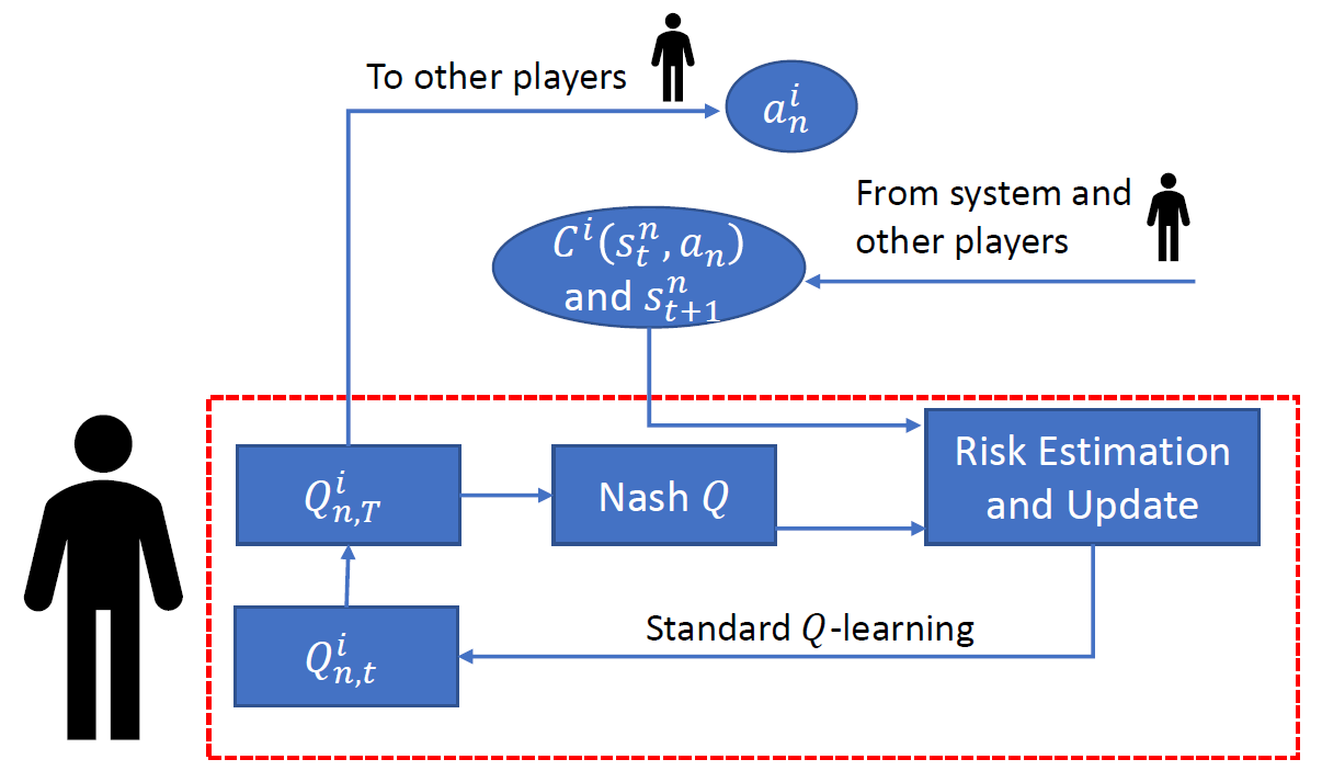
Figure 1: Illustration of RaQL

Each player chooses an action based on a Nash equilibrium of their current $Q$-values, observed cost, other players’ actions, and then the new state in each iteration. The $Q$-values follow a stochastic approximation-type update as in standard $Q$-learning.

Algorithm 1 Risk-aware Nash $Q$-learning

(Step 0) Initialize: Let $n=1$, and $t=1$, get the initial state $s_{1}$. Let the learning agent be indexed by $i$. For all $s\in\mathcal{S}$ and $a^{i}\in\mathcal{A}^{i},\,i\in\mathcal{I}$, let $Q_{n,t}^{i}(s,\,a)=0$.

For $n=1,\,...,\,N$ do

(Step 1) Choose $a_{n}^{i}$ based on the exploration policy $\pi$. Observe the actions and costs for all players, then observe a new state;

      For $t=1,\,...,\,T$ do

      (Step 2) Compute the Nash $Q$-value; Compute the risk-aware cost-to-go for all players;

      (Step 3) Update each $Q_{n,t}^{i},\,i\in\mathcal{I}$ using stochastic approximation;

      (Step 4) Stochastic approximation of risk measure by SASP;

      end for

end for

Return Approximated $Q$-value $Q_{N,T}^{i},\,i\in\mathcal{I}$.

The steps of RaNashQL are summarized in Algorithm 1, which contains $N$ and $T$ number of iterations for outer and inner loops, respectively. In Step 4, we use the stochastic approximation for saddle-point problems (SASP) algorithm, [40, Algorithm 2.1]. Classical stochastic approximation may result in extremely slow convergence for degenerate objectives (i.e. when the objective has a singular Hessian). However, the SASP algorithm with a properly chosen parameter preserves a “reasonable” (close to $O(n^{-1/2})$) convergence rate, even when the objective is non-smooth and/or degenerate. Thus, SASP is a robust choice for solving problem (13). The extended formulations from Steps (0)-(4) in Algorithm 1 are given in the Appendix.

Almost Sure Convergence

Let $\{Q_{n,T}\}_{i\in\mathcal{I}}$ be the $Q$-value estimations at iteration $n$ and $T$ (the end of each inner loop after the risk estimation has been done) from Algorithm 1. We would like to demonstrate the almost sure convergence of $Q_{n,T}^{i}$ to the risk-aware equilibrium $Q$-values $Q_{\ast}^{i}$ for all players. [23] introduce two conditions on the Nash equilibria of all the stage games that lead to almost sure convergence, a global optimal point when every player receives his lowest cost at this point, and a saddle point when each agent would receive a lower cost when at least one of the other players deviates. We found a special type of Nash equilibria that we call an $\mathcal{I}^{\prime}$-mixed point, which builds on [23], and plays a major role in our convergence analysis.

Definition 2.

Let $(C^{i})_{i\in\mathcal{I}}$ denote the expected cost of all players as a function of the multi-strategy $x\in\mathcal{X}$. A multi-strategy $x\in\mathcal{X}$ is a $\mathcal{I}^{\prime}$-mixed point of $\left(C^{i}\right)_{i\in\mathcal{I}}$ if: (i) it is a Nash equilibrium and (ii) there exists an index of players $\mathcal{I}^{\prime}\subseteq\mathcal{I}$ such that: $C^{i}\left(x\right)\leq C^{i}\left(x^{\prime}\right),\,\forall x^{\prime}\in\mathcal{X},\,i\in\mathcal{I}^{\prime}$, and $C^{i}\left(x^{i},\,x^{-i}\right)\leq C^{i}\left(x^{i},\,u^{-i}\right),\,\forall u^{-i}\in\mathcal{X}^{-i},\,i\in\mathcal{I}\backslash\mathcal{I}^{\prime}$.

Our definition of ‘$\mathcal{I}^{\prime}$-mixed point’ combines both notions of global optimal point and saddle point. From Definition 2, a subset of players $\mathcal{I}^{\prime}\subseteq\mathcal{I}$ minimizes their expected costs at $x$. The rest of the players $\mathcal{I}\backslash\mathcal{I}^{\prime}$ each would receive a lower expected cost when at least one of the other players deviates. An example of an $\mathcal{I}^{\prime}$-mixed point in a one shot game follows.

Example 2.

Player 1 has choices Up and Down, and Player 2 has choices Left and Right. Player 1’s loss is the first entry in each cell, and Player 2’s are the second. The first game has a unique Nash equilibrium (Up, Left), which is a global optimal point. The second game also has a unique Nash equilibrium (Down, Right), which is a saddle-point. The third game has two Nash equilibrium: a global optimum (Up, Left), and a mixed point (Down, Right). In equilibrium (Down, Right), Player 1 receives a lower cost if Player 2 deviates, while Player 2 receives a higher cost if Player 1 deviates.

Game 1	Left	Right
Up	$0,\,1$	$10,\,7$
Down	$7,\,10$	$11,\,8$

Game 2	Left	Right
Up	$5,\,5$	$10,\,4$
Down	$4,\,10$	$8,\,8$

Game 3	Left	Right
Up	$0,\,1$	$10,\,9$
Down	$7,\,10$	$8,\,8$

Table 1: Examples of $\mathcal{I}^{\prime}$-mixed point

We now introduce the following additional assumptions for our analysis of RaNashQL.

Assumption 3.

One of the following holds for all stage games $(Q_{n,T}^{i}(s))_{i\in\mathcal{I}}$ for all $n$ and $s\in\mathcal{S}$ in Algorithm 1.

(i) Every $(Q_{n,T}^{i}(s))_{i\in\mathcal{I}}$ for all $n$ and $s\in\mathcal{S}$ has a global optimal point.

(ii) Every $(Q_{n,T}^{i}(s))_{i\in\mathcal{I}}$ for all $n$ and $s\in\mathcal{S}$ has a saddle point.

(iii) For any two stage games $Q,\,\tilde{Q}\in(Q_{n,T}^{i}(s))_{i\in\mathcal{I}}$ for all $n$ and $s\in\mathcal{S}$, we suppose $Q_{1}$ has a $\mathcal{I}_{1}$-mixed point $x$ and $Q_{2}$ has a $\mathcal{I}_{2}$-mixed point $\tilde{x}$. Then: For $i\in\mathcal{I}_{1}\cup(\mathcal{I}\backslash\mathcal{I}_{2})$, then $Q^{i}\left(x\right)\geq\tilde{Q}^{i}\left(\tilde{x}\right)$; For $i\in\mathcal{I}_{2}\cup(\mathcal{I}\backslash\mathcal{I}_{1})$, then $Q^{i}\left(x\right)\leq\tilde{Q}^{i}\left(\tilde{x}\right)$.

Compared with [23, Assumption 3], Assumption 3(iii) enables wider application of RaNashQL. In particular, even the indices $\mathcal{I}_{1}$ and $\mathcal{I}_{2}$ of all the stage games may differ across iterations. Next we list further standard assumptions on exploration in RaNashQL and its asynchronous updates.

Assumption 4.

(i) The exploration policy $\pi$ is $\varepsilon-$greedy, meaning with probability $\varepsilon\in\left(0,\,1\right)$, action $a^{i}$ is chosen uniformly from $\mathcal{A}^{i}$, and with probability $1-\varepsilon$, action $a^{i}$ is drawn from $\mathcal{A}^{i}$ according to $x_{s}^{i}$ which is the equilibrium of the stage game $\{Q^{i}(s)\}_{i\in\mathcal{I}}$; (ii) a single state-action pair is updated when it is observed in each iteration.

By the Extended Borel-Cantelli Lemma [11], the algorithm satisfying Assumption 4(i) will visit every state-action pair infinitely often with probability one.

Theorem 2.

Suppose Assumptions 3 and 4 hold. For any $T\geq 1$, Algorithm 1 generates sequences $\left\{Q_{n,T}^{i}\right\}_{n\geq 1}$ such that $Q_{n,\,T}^{i}\rightarrow Q_{\ast}^{i}$ almost surely as $n\rightarrow\infty$ for all $i\in\mathcal{I}$.

Proof.

(Proof sketch) (i) Show that all $\mathcal{I}^{\prime}$-mixed points of a stage game have equal value, and the property also holds for global optimal points and saddle points. Consequently, from [23], the mapping from $Q$-values to Nash equilibrium (of the stage games) is non-expansive.

(ii) Show that the Hausdorff distance between the subdifferentials of the estimated risk on $\mathcal{Y}^{i}$ and $\mathcal{Z}^{i}$ (corresponding to Eq. (13)), is bounded by a function of $\|Q_{n-1,T}^{i}-Q_{\ast}^{i}\|_{2}$.

(iii) Show that the duality gaps of all the saddle point estimation problems are bounded by a function of $\|Q_{n-1,T}^{i}-Q_{\ast}^{i}\|_{2}$.

(iv) If the conditions in (i)-(iii) hold, then $Q_{n,\,T}^{i}$ from RaNashQL are a well-behaved stochastic approximation sequence [15, Definition 7] that converges to $Q_{\ast}^{i}$ with probability one. ∎

The full proof Theorem 2 is presented in the Appendix.

[26, Theorem 4.7] shows that the single-agent version of RaNashQL has complexity

$$\Omega\left(\left(S\,A\ln(S\,A/\delta\epsilon)/\epsilon^{2}\right)^{1/\beta}+(\ln(\sqrt{S\,A}/\epsilon))^{1/(1-\beta)}\right),$$ (16)

with probability $1-\delta$, where $S$ and $A$ denote the cardinality of state and actions spaces and $\beta\in(0,\,1]$ is the learning rate. In the multi-agent case, our conjecture is to replace $A$ with $|\mathcal{A}|$ in the term (16) to get a rough estimate of the time complexity of RaNashQL. However, the explicit complexity bound is difficult to derive and remains for future research. In RaNashQL, there are multiple $Q$-values being updated in each iteration for each state, and their relationships are complex (they are linked by the solutions of a stage game, since each stage game may yield multiple Nash equilibria).

In the Appendix, we also discuss (i) methods for computing Nash equilibria of stage games involving two or more players; (ii) a rule for choosing a unique Nash equilibrium of stage games from multiple choices; (iii) the storage space requirement of RaNashQL.

4 A Queuing Control Application

We apply our techniques to the single server exponential queuing system from [30]. In this packet switched network, it is service provider’s (denoted as “SP” latter in the tables) benefit to increase the amount of packets processed in the system. However, such an increase may result in an increase in packets’ waiting times in the buffer (called latency), and routers (denoted as “R” latter in the tables) are used to reduce packets’ waiting times. Thus, the game arises because the service provider and router choose their service rates to achieve competing objectives.

The state space $\mathcal{S}$ represents the maximum number ($30$ in these experiments) of packets allowed in the system. We assume that the time until the admission of a new packet and the next service completion are both exponentially distributed. Therefore, the number of packets in the system can be modeled as a birth and death process with fixed state transition probabilities. In the Appendix, we provide the explicit formulation of cost functions, state transition probabilities, as well as other parameter settings. We suppose that each player has the same two available actions (service rates) in every state. CVaR is the risk measure for both players in all the experiments. The player’s risk preferences are obtained by setting $\alpha^{i}$ for $i=1,2$, and we allow $\alpha^{1}\neq\alpha^{2}$.

Experiment I (RaNashQL vs. Nash $Q$-learning)

We compare RaNashQL with Nash $Q$-learning in [23] in terms of their convergence rates. Given any precision $\epsilon>0$, we record the iteration count $n$ until the convergence criterion $\|Q_{n,\,T}^{i}-Q_{\ast}^{i}\|_{2}\leq\epsilon$ is satisfied. Figure 2 (top) reveals that RaNashQL is more computationally expensive than Nash $Q$-learning. Table 2 shows the discounted cost under equilibrium by simulation (1000 samples). The first table reveals that incorporating risk will help the service provider reduce its mean cost, while increase the mean cost of the router. The second table shows that incorporating risk will help to reduce the overall cost to the entire system with only a slightly higher variance.

The first part of Table 3 shows that the mean cost of service provider ($-44.31$) is lower than that under the risk-neutral Markov perfect equilibrium ($-22.22$), and the mean cost of router ($59.64$) is lower than that under the risk-aware Markov perfect equilibrium ($37.48$). This result shows that incorporating risk preference can help decision makers reach a new equilibrium that further reduces his mean cost compared to cases where both players are either risk-neutral or risk-aware. Similar phenomena can also be shown in the second part of Table 3. In the final part of Table 3, we construct a new two-player one-shot game where the risk preferences (risk-neutral and risk-aware) are the actions and the expected value from simulation will be outcome of the game. We find that a equilibrium is attained for this game when the router is risk-neutral and the service provider is risk-aware. This one-shot game demonstrates that the router should be risk-neutral when service provider is risk-aware, in order to reduce his expected cost.

In the Appendix, we further explain the reason for the increase in variance in risk-aware games in Table 2 which is counter-intuitive.

Player	Method	Mean	Variance	$5$%-CVaR	$10$%-CVaR
SP	Neutral	$-22.22$	$1.4736e-06$	$-22.22$	$-22.22$
	CVaR	$-77.78$	$407.84$	$-69.34$	$-68.26$
R	Neutral	$37.48$	$7.32$	$37.94$	$38.18$
	CVaR	$83.68$	$491.20$	$86.03$	$87.54$

Method	Mean	$5$%-CVaR	10%-CVaR
Neutral	15.26	15.72	15.96
CVaR	5.9	16.69	19.28

Table 2: Simulation (Constructing CVaR with $\alpha^{1}=\alpha^{2}=0.1$)

Player	Method	Mean	Variance	$5$%-CVaR	$10$%-CVaR
SP	CVaR	$-44.31$	$266.06$	$-43.38$	$-42.70$
R	Neutral	$59.64$	$316.71$	$61.18$	$62.77$

Player	Method	Mean	Variance	$5$%-CVaR	$10$%-CVaR
SP	CVaR	$-54.76$	$26.05$	$-54.71$	$-54.67$
R	Neutral	$70.56$	$31.03$	$71.56$	$71.81$

		Router
		Risk-neutral	Risk-aware
Service Provider	Risk-neutral	$(-22.22,37.48)$	$(-54.76,70.56)$
	Risk-aware	$(-44.44,59.64)$	$(-77.78,83.68)$

Table 3: Simulation ( Constructing CVaR with $\alpha^{1}=0.95$, $\alpha^{2}=0.1$ for the first table, and $\alpha^{1}=0.1$, $\alpha^{2}=0.95$ for the second)

Experiment II (RaNashQL vs. Multilinear System)

In this experiment, we consider a special case where the risk only comes from state transitions (this setting is basically a risk-aware interpretation of [30]). In this case, we can compute the risk-aware Markov equilibrium “exactly” using a multilinear system and interior point algorithm as detailed in the Appendix. We evaluate performance in terms of the relative error

$$\frac{\sqrt{\sum_{s\in\mathcal{S}}\left(Nash^{i}(Q_{n,\,T}^{j}(s))_{j\in\mathcal{I}}-v_{\ast}^{i}(s)\right)^{2}}}{\sqrt{\sum_{s\in\mathcal{S}}v_{\ast}^{i}(s)^{2}}},\,n\leq N,$$

where $v_{\ast}^{i}$ is the value function corresponding to the equilibrium solved by multilinear system. The Appendix confirms that the service provider’s strategy produced by RaNashQL converges almost surely to the one produced by multilinear system. From the Appendix, interior point algorithm finds a local optimum with 10471.975 seconds, and RaNashQL has relative error lower than 25% with 5122.657 seconds. Thus, our approach possesses superior computational performance compared to an interior point algorithm for solving multilinear systems.

Experiment III (Computational Complexity Conjecture)

In this experiment, we explore the conjecture on the computational complexity of RaNashQL. Given a fixed $\epsilon$, we could compute the complexity conjecture through formulation (16). Figure 2 (bottom) shows that the relative errors of service provider and router under computed complexity conjecture are bounded by $\epsilon$. Thus we derive a potential heuristic for the computational complexity of solving a general sum game given the size of the game. In other words, each practitioner can estimate the upper bound of total complexity in computing the $\epsilon-$ equilibrium through this conjecture.

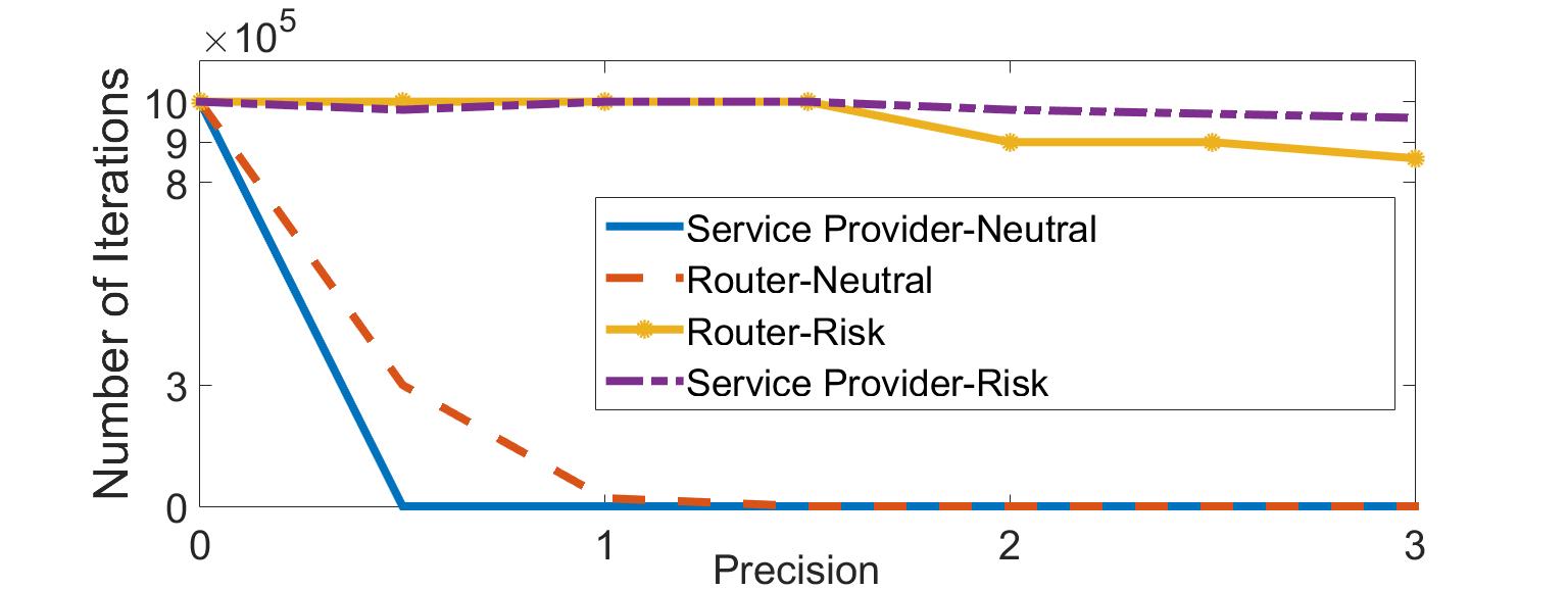
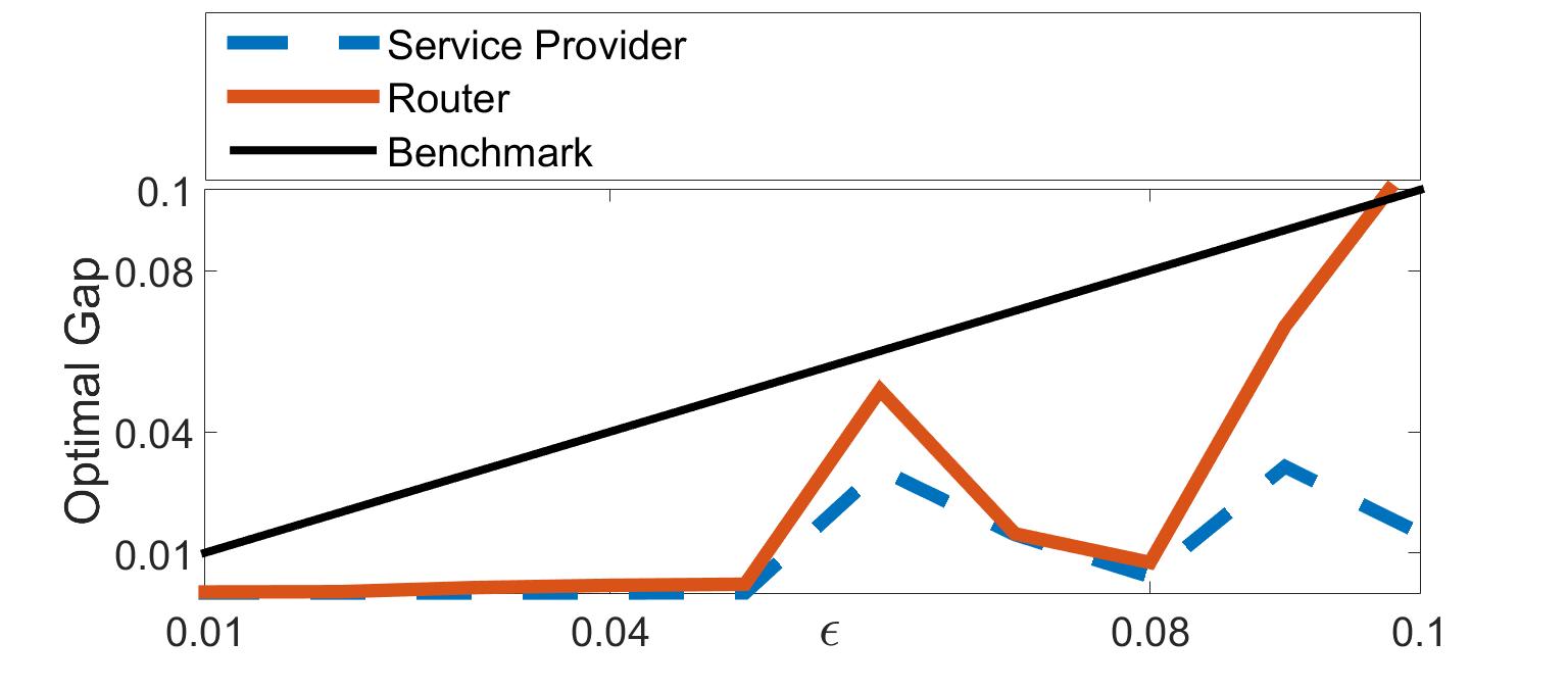
Figure 2: Computational Complexity

5 Conclusion

In this paper, we propose a model and simulation-based algorithm for non-cooperative Markov games with time-consistent risk-aware players. This work has made the following contributions: (i) The model characterizes the “risk” from both the stochastic state transitions and the randomized strategies of the other players. (ii) We define risk-aware Markov perfect equilibrium and prove its existence in stationary strategies. (iii) We show that our algorithm converges to risk-aware Markov perfect equilibrium almost surely. (iv) From a queuing control numerical example, we find that risk-aware Markov games will reach new equilibria other than risk-neutral ones (this is the equilibrium shifting phenomenon). Moreover, the variance is increased for risk-aware Markov games, which is contrary to the variance reduction property of risk-aware optimization for single agents. The sum of expected cost over all players is reduced in risk-aware Markov game, compared to risk-neutral ones. In future research, we seek to improve the scalability of our framework for large-scale Markov games.

Appendix A Appendix

A.1 Dynamic Risk Measures

In this section, we describe the risk measures in our risk-aware Markov games. In our model, each player $i$ faces a sequence of costs $X_{t}=c^{i}(s_{t},\,a_{t})$ for all $t\geq 0$. There are two sources of stochasticity in this cost sequence: (i) stochastic state transitions characterized by the transition kernel $P(\cdot\,|\,s,\,a)$; and (ii) the randomized mixed strategies of other players characterized by $x^{-i}$. The key question is: how should player $i$ account for both sources of stochasticity and evaluate the risk of the tail subsequence $X_{t},\,X_{t+1},\ldots$ from the perspective of time $t$?

We begin by formalizing some details about the risk of finite cost sequences $X_{t,\,T}:=(X_{t},\,X_{t+1},\ldots,\,X_{T})$ before we consider the risk of the infinite cost sequence $X_{0},\,X_{1},\ldots$ actually faced by the players. For a reference distribution $P$ on $\left(\Omega,\,\mathcal{F}\right)$, and we define $L_{t}:=\mathcal{L}_{\infty}(\Omega,\mathcal{\,F}_{t},\,P)$ and $L_{t,\,T}:=L_{t}\times L_{t+1}\times\cdots\times L_{T}$ for all $0\leq t\leq T<\infty$.

Definition 3.

(i) A mapping $\rho_{t,\,T}:\,L_{t,\,T}\rightarrow L_{t}$, is called a conditional risk measure if: $\rho_{t,\,T}(Z_{t,\,T})\leq\rho_{t,\,T}(X_{t,\,T})$ for all $Z_{t,\,T},\,X_{t,\,T}\in L_{t,\,T}$ such that $Z_{t,\,T}\leq X_{t,\,T}$.

(ii) A dynamic risk measure is a sequence of conditional risk measures $\{\rho_{t,\,T}\}_{t=0}^{T}$.

Given a dynamic risk measure $\{\rho_{t,\,T}\}_{t=0}^{T}$, we may define a larger family of risk measures $\rho_{t,\,\tau}$ for $0\leq t\leq\tau\leq T$ via the convention $\rho_{t,\,\tau}(X_{t},\ldots,\,X_{\tau})=\rho_{t,\,\tau}(X_{t},\ldots,\,X_{\tau},\,0,\ldots,\,0)$.

We now make our key assumptions about player risk preferences.

Assumption 5.

The dynamic risk measure $\{\rho_{t,\,T}\}_{t=0}^{T}$ satisfies the following conditions:

(i) (Normalization) $\rho_{t,\,T}(0,\,0,\,...,\,0)=0.$

(ii) (Conditional translation invariance) For any $X_{t,\,T}\in L_{t,\,T}$,

$$\rho_{t,\,T}(X_{t},\,X_{t+1},\,...,\,X_{T})=X_{t}+\rho_{t,\,T}(0,\,X_{t+1},\,...,\,X_{T}).$$

(iii) (Convexity) For any $X_{t,\,T},\,Y_{t,\,T}\in L_{t,\,T}$ and $0\leq\lambda\leq 1$, $\rho_{t,\,T}(\lambda\,X_{t,\,T}+(1-\lambda)Y_{t,\,T})\leq\lambda\,\rho_{t,\,T}(X_{t,\,T})+(1-\lambda)\rho_{t,\,T}(Y_{t,\,T})$.

(iv) (Positive homogeneity) For any $X_{t,\,T}\in L_{t,\,T}$ and $\alpha\geq 0$, $\rho_{t,\,T}(\alpha\,X_{t,\,T})=\alpha\,\rho_{t,\,T}(X_{t,\,T}).$

(v) (Time-consistency) For any $X_{t,\,T},\,Y_{t,\,T}\in L_{t,\,T}$ and $0\leq\tau\leq\theta\leq T$, the conditions $X_{k}=Y_{k}$ for $k=\tau,\,...,\,\theta-1$ and $\rho_{\theta,\,T}(X_{\theta},\,....,\,X_{T})\leq\rho_{\theta,\,T}(Y_{\theta},\,...,\,Y_{T})$ imply $\rho_{\tau,\,T}(X_{\tau},\,....,\,X_{T})\leq\rho_{\tau,\,T}(Y_{\tau},\,...,\,Y_{T})$.

Many of these properties (monotonicity, convexity, positive homogeneity, and translation invariance) were originally introduced for static risk measures in the pioneering paper [2]. They have since been heavily justified in other works including [46, 8, 39].

The next theorem gives a recursive formulation for dynamic risk measures satisfying Assumption 5. This representation is the foundation of [44] and subsequent works on time-consistent risk measures. For this result, we define a mapping $\rho_{t}\text{ : }L_{t+1}\rightarrow L_{t}$, where $t\geq 0$, to be a one-step (conditional) risk measure if $\rho_{t}(X_{t+1})=\rho_{t,\,t+1}(0,\,X_{t+1})$.

Theorem 3.

[44, Theorem 1] Suppose Assumption 5 holds, then

$$\rho_{t,\,T}(X_{t},\,X_{t+1},...,\,X_{T},\ldots)=X_{t}+\rho_{t}(X_{t+1}+\rho_{t+1}(X_{t+2}+\cdot\cdot\cdot+\rho_{T}(X_{T})+\cdot\cdot\cdot)),$$ (17)

for all $0\leq t\leq T$, where $\rho_{t},\ldots,\,\rho_{T}$ are one-step conditional risk measures.

Now we may consider the risk of an infinite cost sequence. Based on [44], the discounted measure of risk $\rho_{t,\,T}^{\gamma}\text{ : }L_{t,\,T}\rightarrow\mathbb{R}$ is defined via

$$\rho_{t,\,T}^{\gamma}(X_{t},\,X_{t+1},\ldots,\,X_{T}):=\rho_{t,\,T}(\gamma^{t}X_{t},\,\gamma^{t+1}X_{t+1},\ldots,\,\gamma^{T}X_{T}).$$

Define $L_{t,\,\infty}:=L_{t}\times L_{t+1}\times\cdot\cdot\cdot$ for $t\geq 0$ and $\rho^{\gamma}\text{ : }L_{0,\,\infty}\rightarrow\mathbb{R}$ via

$$\rho^{\gamma}(X_{0},\,X_{1},\ldots):=\lim_{T\rightarrow\infty}\rho_{0,\,T}^{\gamma}(X_{0},\,X_{1},\ldots,\,X_{T}).$$

To provide our final representation result, we introduce the additional assumption that player risk preferences are stationary (they only depend on the sequence of costs ahead, and are independent of the current time).

Assumption 6.

(Stationary risk preferences) For all $T\geq 1$ and $s\geq 0$,

$$\rho_{0,\,T}^{\gamma}(X_{0},\,X_{1},\ldots,\,X_{T})=\rho_{s,\,T+s}^{\gamma}(X_{0},\,X_{1},\ldots,\,X_{T}).$$

When Assumptions 5 and 6 are satisfied, the corresponding dynamic risk measure is given by the recursion:

$$\rho^{\gamma}(X_{0},\,X_{1},...,\,X_{T},\ldots)=X_{0}+\rho_{1}(\gamma X_{1}+\rho_{2}(\gamma^{2}X_{2}+\cdot\cdot\cdot+\rho_{T}(\gamma^{T}X_{T})+\cdot\cdot\cdot)),$$ (18)

where $\rho_{1},\,\rho_{2},\ldots$ are all one-step risk measures. Based on representation (18), we may define the risk-aware objective for player $i$ to be:

$$J_{s_{0}}^{i}(x^{i},\,x^{-i})=\rho^{i}(c^{i}(s_{0},\,a_{0})+\gamma\,\rho^{i}(c^{i}(s_{1},\,a_{1})+\gamma\,\rho^{i}(c^{i}(s_{2},\,a_{2})+\cdot\cdot\cdot))).$$ (19)

where $\rho^{i}$ is a one-step conditional risk measure that maps random cost from the next stage to current stage, with respect to the joint distribution of randomized mixed strategies and transition kernels. In formulation (19), each $c^{i}(s_{t},\,a_{t}),\,t\geq 1$ is governed by the joint distribution of randomized mixed strategies and transition kernel

$$\times_{i\in\mathcal{I}}~{}x_{s_{t}}^{i}(a_{t}^{i})P(s_{t}|s_{t-1},\,a_{t-1}),$$

which is defined for fixed $(s_{t-1},\,a_{t-1})$ and for all $s_{t}$ and $a_{t}^{i}$. The distribution of $c^{i}$ is only governed by $\times_{i\in\mathcal{I}}~{}x_{s_{0}}^{i}(a_{0}^{i})$.

A.2 Proof of Theorem 1

Fundamental Inequalities

We make heavy use of the following fundamental inequalities and algebraic identity.

Fact 1.

Let $\mathcal{X}$ be a nonempty set and $f_{1},\,f_{2}\text{ : }\mathcal{X}\rightarrow\mathbb{R}$ be functions on $\mathcal{X}$.

(i) $|\min_{x\in\mathcal{X}}f_{1}\left(x\right)-\min_{x\in\mathcal{X}}f_{2}\left(x\right)|\leq\max_{x\in\mathcal{X}}|f_{1}\left(x\right)-f_{2}\left(x\right)|$.

(ii) $|\max_{x\in\mathcal{X}}f_{1}\left(x\right)-\max_{x\in\mathcal{X}}f_{2}\left(x\right)|\leq\max_{x\in\mathcal{X}}|f_{1}\left(x\right)-f_{2}\left(x\right)|$.

Proof.

For part (i), we compute

$$\min_{x\in\mathcal{X}}f_{1}\left(x\right)=\, \min_{x\in\mathcal{X}}\left(f_{1}\left(x\right)-f_{2}\left(x\right)+f_{2}\left(x\right)\right)$$

$$\leq\, \min_{x\in\mathcal{X}}\left(f_{2}\left(x\right)+|f_{1}\left(x\right)-f_{2}\left(x\right)|\right)$$

$$\leq\, \min_{x\in\mathcal{X}}f_{2}\left(x\right)+\max_{x\in\mathcal{X}}|f_{1}\left(x\right)-f_{2}\left(x\right)|$$

which gives

$$\min_{x\in\mathcal{X}}f_{1}\left(x\right)-\min_{x\in\mathcal{X}}f_{2}\left(x\right)\leq\max_{x\in\mathcal{X}}|f_{1}\left(x\right)-f_{2}\left(x\right)|.$$

By a symmetric argument, we have

$$\min_{x\in\mathcal{X}}f_{2}\left(x\right)-\min_{x\in\mathcal{X}}f_{1}\left(x\right)\leq\max_{x\in\mathcal{X}}|f_{1}\left(x\right)-f_{2}\left(x\right)|,$$

from which the desired conclusion follows. The proof for part (ii) is similar. ∎

Define $d_{\mathcal{H}}(\mathfrak{A},\,\mathfrak{B}\text{)}$ to be the Hausdorff distance between nonempty subsets $\mathfrak{A}$ and $\mathfrak{B}$ of $\mathbb{R}^{d}$ with respect to the Euclidean norm $\|\cdot\|_{2}$, explicitly,

$$d_{\mathcal{H}}(\mathfrak{A},\,\mathfrak{B}\text{)}:=\max\left\{\sup_{a\in\mathfrak{A}}\inf_{b\in\mathfrak{B}}\|a-b\|_{2},\,\sup_{b\in\mathfrak{B}}\inf_{a\in\mathfrak{A}}\|a-b\|_{2}\right\}.$$

Fact 2.

Let $\left(\mathcal{X},\,\|\cdot\|\right)$ be a normed space, $f\text{ : }\mathcal{X}\rightarrow\mathbb{R}$ be an $L_{f}$-Lipschitz function, and $\mathcal{X}_{1},\,\mathcal{X}_{2}\subset\mathcal{X}$. Then

$$|\min_{x\in\mathcal{X}_{1}}f\left(x\right)-\min_{x\in\mathcal{X}_{2}}f\left(x\right)|\leq L_{f}d_{\mathcal{H}}(\mathcal{X}_{1},\,\mathcal{X}_{2}).$$

Proof.

Let $x_{1}^{*}\in\mathcal{X}_{1}$ be an optimal solution of $\min_{x\in\mathcal{X}_{1}}f\left(x\right)$. There is an $x_{2}\in\mathcal{X}_{2}$ by definition of $d_{\mathcal{H}}$such that $\|x_{1}^{*}-x_{2}\|\leq d_{\mathcal{H}}(\mathcal{X}_{1},\,\mathcal{X}_{2})$, and so

$$\min_{x\in\mathcal{X}_{2}}f\left(x\right)\leq f(x_{2})\leq f(x_{1}^{*})+L_{f}d_{\mathcal{H}}(\mathcal{X}_{1},\,\mathcal{X}_{2})=\min_{x\in\mathcal{X}_{1}}f(x_{1})+L_{f}d_{\mathcal{H}}(\mathcal{X}_{1},\,\mathcal{X}_{2}),$$

where the second inequality follows by $L_{f}$-Lipschitz continuity of $f$. The other direction follows by symmetric reasoning. ∎

Fact 3.

Define

$$\delta_{0}(\epsilon):=\frac{\min\{\epsilon,\,1\}}{(2^{|\mathcal{I}|}-1)|\mathcal{A}|},$$

then $\left|\Pi_{i\in\mathcal{I}}x_{s}^{i}(a^{i})-\Pi_{i\in\mathcal{I}}y_{s}^{i}(a^{i})\right|\leq\epsilon$ holds for any $x,\,y\in\mathcal{X}$.

Proof.

We make use of the following algebraic identity

$$\left|\Pi_{i\in\mathcal{I}}x_{s}^{i}(a^{i})-\Pi_{i\in\mathcal{I}}y_{s}^{i}(a^{i})\right|$$

$$= \left|\sum_{\left\{\Omega\subset\mathcal{I},\,\Omega\neq\emptyset\right\}}\left(\prod_{\begin{array}[]{c}i\in\Omega\end{array}}(x_{s}^{i}(a^{i})-y_{s}^{i}(a^{i})\right)\left(\prod_{\begin{array}[]{c}i\notin\Omega\end{array}}y_{s}^{i}(a^{i})\right)\right|$$

$$\leq \sum_{\left\{\Omega\subset\mathcal{I},\,\Omega\neq\emptyset\right\}}\left|\prod_{\begin{array}[]{c}i\in\Omega\end{array}}(x_{s}^{i}(a^{i})-y_{s}^{i}(a^{i})\right|$$

$$\leq \sum_{\left\{\Omega\subset\mathcal{I},\,\Omega\neq\emptyset\right\}}\left(\delta_{0}(\epsilon)\right)^{|\Omega|}$$

$$\leq \sum_{\left\{\Omega\subset\mathcal{I},\,\Omega\neq\emptyset\right\}}\delta_{0}(\epsilon)$$

$$= \epsilon.$$

∎

Existence of Stationary Equilibria

This section develops the machinery for our proof of Theorem 1, which is based on Kakutani’s fixed point theorem.

Theorem 4.

[29] (Kakutani’s fixed point theorem) If $\mathcal{X}$ is a closed, bounded, and convex set in Euclidean space, and $\Phi$ is an upper semicontinuous correspondence mapping from $\mathcal{X}$ into the family of closed, convex subsets of $\mathcal{X}$, then there exists an element $x\in\mathcal{X}$ such that $x\in\Phi(x)$.

For a multi-strategy $x\in\mathcal{X}$, we define the operator $\mathcal{T}_{x}:\,\mathcal{V}\to\mathcal{V}$ via

$$[\mathcal{T}_{x}(v)]_{s}^{i}:=\min_{u_{s}^{i}\in\mathcal{P}\left(\mathcal{A}^{i}\right)}\{\rho^{i}\left(c^{i}(s\,,A)+\gamma\,v^{i}\left(S^{\prime}\right)\right)\text{ : }(A,\,S^{\prime})\sim P_{s}(u_{s}^{i},\,x_{s}^{-i})\},\,\forall i\in\mathcal{I},\,s\in\mathcal{S}.$$

For simplification, we define, for any $v\in\mathcal{V}$, $i\in\mathcal{I}$ and $s\in\mathcal{S}$,

$$\psi_{s}^{i}(u_{s}^{i},\,x_{s}^{-i},\,v^{i}):=\rho^{i}\left(c^{i}(s\,,A)+\gamma\,v^{i}\left(S^{\prime}\right)\right),\,(A,\,S^{\prime})\sim P_{s}(u_{s}^{i},\,x_{s}^{-i}).$$

Our proof of Theorem 1 has three main steps:

1. (Step 1) Show that $\mathcal{T}_{x}$ is a contraction.

2. (Step 2) Show that the cost-to-go function $\psi_{s}^{i}(u_{s}^{i},\,x_{s}^{-i},\,v^{i})$ is continuous.

3. (Step 3) Verify that the assumptions of Kakutani’s fixed point theorem are met for $\Phi$.

Step 1: Show that $\mathcal{T}_{x}$ is a contraction

We establish that the operator $\mathcal{T}_{x}$ is a contraction, and subsequently that given any stationary strategy $x$, there is a corresponding unique value function $v^{i}$ for all players.

Proposition 1.

For each $x\in\mathcal{X}$, $\mathcal{T}_{x}$ is a contraction with constant $\gamma\in\left(0,\,1\right)$.

Proof.

Let $v,\,w\in\mathcal{V}$. For $i\in\mathcal{I}$ and $s\in\mathcal{S}$, let $g_{s}^{i}$ attain the minimum in the definition of $\left[\mathcal{T}_{x}(v)\right]_{s}^{i}$,

$$[\mathcal{T}_{x}(v)]_{s}^{i}=\min_{u_{s}^{i}\in\mathcal{P}(\mathcal{A}^{i})}\psi_{s}^{i}\left(u_{s}^{i},\,x_{s}^{-i},\,v^{i}\right)=\sup_{\mu\in\mathcal{M}_{s}^{i}(P_{s}(g_{s}^{i},\,x_{s}^{-i}))}\left\{\langle\mu,\,C_{s}^{i}(v^{i})\rangle-\alpha_{s}^{i}(\mu)\right\}.$$

Similarly, let $z_{s}^{i}$ attain the minimum in $\left[\mathcal{T}_{x}(w)\right]_{s}^{i}$,

$$[\mathcal{T}_{x}(w)]_{s}^{i}=\sup_{\mu\in\mathcal{M}_{s}^{i}(P_{s}(z_{s}^{i},\,x_{s}^{-i}))}\left\{\langle\mu,\,C_{s}^{i}(w^{i})\rangle-\alpha_{s}^{i}(\mu)\right\}.$$

It follows that

$$[\mathcal{T}_{x}(v)]_{s}^{i}-[\mathcal{T}_{x}(w)]_{s}^{i}$$

$$=\, \sup_{\mu\in\mathcal{M}_{s}^{i}(P_{s}(g_{s}^{i},\,x_{s}^{-i}))}\left\{\langle\mu,\,C_{s}^{i}(v^{i})\rangle-\alpha_{s}^{i}(\mu)\right\}-\sup_{\mu\in\mathcal{M}_{s}^{i}(P_{s}(z_{s}^{i},\,x_{s}^{-i}))}\left\{\langle\mu,\,C_{s}^{i}(w^{i})\rangle-\alpha_{s}^{i}(\mu)\right\}$$

$$\leq\, \sup_{\mu\in\mathcal{M}_{s}^{i}(P_{s}(z_{s}^{i},\,x_{s}^{-i}))}\left\{\langle\mu,\,C_{s}^{i}(v^{i})\rangle-\alpha_{s}^{i}(\mu)\right\}-\sup_{\mu\in\mathcal{M}_{s}^{i}(P_{s}(z_{s}^{i},\,x_{s}^{-i}))}\left\{\langle\mu,\,C_{s}^{i}(w^{i})\rangle-\alpha_{s}^{i}(\mu)\right\}$$

$$\leq\, \gamma\sup_{\mu\in\mathcal{M}_{s}^{i}(P_{s}(z_{s}^{i},\,x_{s}^{-i}))}\sum_{\left(a,\,s^{\prime}\right)\in\mathcal{K}}\mu\left(a,\,s^{\prime}\right)|v^{i}\left(s^{\prime}\right)-w^{i}\left(s^{\prime}\right)|$$

$$\leq\, \gamma\|v-w\|_{\infty},$$

where the first inequality holds by choice of $g_{s}^{i}$. The argument to upper bound $[\mathcal{T}_{x}(w)]_{s}^{i}-[\mathcal{T}_{x}(v)]_{s}^{i}$ is symmetric. ∎

Since $(\mathcal{V},\,\|\cdot\|_{\infty})$ is a complete metric space and $\mathcal{T}_{x}$ is a contraction mapping on $\mathcal{V}$ by Proposition 1, $\mathcal{T}_{x}$ has a unique fixed point by the Banach fixed point theorem.

Proposition 2.

For any stationary strategy $x\in\mathcal{X}$, there exists a unique value function $v\in\mathcal{V}$ such that $\forall s\in\mathcal{S},\,i\in\mathcal{I}$,

$$v^{i}\left(s\right)=\min_{u_{s}^{i}\in\mathcal{P}\left(\mathcal{A}^{i}\right)}\rho^{i}(c^{i}(s,\,A)+\gamma\,v^{i}\left(S^{\prime}\right))=\min_{u_{s}^{i}\in\mathcal{P}\left(\mathcal{A}^{i}\right)}\psi_{s}^{i}(u_{s}^{i},\,x_{s}^{-i},\,v^{i}).$$

Step 2: Show that $\psi_{s}^{i}$ is continuous

We want to establish continuity of $\psi_{s}^{i}\left(x_{s}^{i},\,x_{s}^{-i},\,v^{i}\right)$ in all its arguments for all $i\in\mathcal{I}$ and $s\in\mathcal{S}$. Firstly, we know that the function $(\mu,\,v^{i})\rightarrow\langle\mu,\,C_{s}^{i}(v^{i})\rangle-\alpha_{s}^{i}(\mu)$ is Lipschitz continuous based on Assumption 1. We use $L$ to denote the Lipschitz constant. Our argument is based on the following chain of inequalities:

$$|\psi_{s}^{i}(x_{s}^{i},\,x_{s}^{-i},\,v^{i})-\psi_{s}^{i}(y_{s}^{i},\,y_{s}^{-i},\,w^{i})|$$

$$\leq\, |\psi_{s}^{i}(x_{s}^{i},\,x_{s}^{-i},\,v^{i})-\psi_{s}^{i}(x_{s}^{i},\,x_{s}^{-i},\,w^{i})|+|\psi_{s}^{i}(x_{s}^{i},\,x_{s}^{-i},\,w^{i})-\psi_{s}^{i}(y_{s}^{i},\,y_{s}^{-i},\,w^{i})|$$

$$\leq\, |\sup_{\mu\in\mathcal{M}_{s}^{i}(P_{s}(x_{s}))}\left\{\langle\mu,\,C_{s}^{i}(v^{i})\rangle-\alpha_{s}^{i}(\mu)\right\}-\sup_{\mu\in\mathcal{M}_{s}^{i}(P_{s}(x_{s}))}\left\{\langle\mu,\,C_{s}^{i}(w^{i})\rangle-\alpha_{s}^{i}(\mu)\right\}|$$

$$+|\sup_{\mu\in\mathcal{M}_{s}^{i}(P_{s}(x_{s}))}\left\{\langle\mu,\,C_{s}^{i}(w^{i})\rangle-\alpha_{s}^{i}(\mu)\right\}-\sup_{\mu\in\mathcal{M}_{s}^{i}(P_{s}(y_{s}))}\left\{\langle\mu,\,C_{s}^{i}(w^{i})\rangle-\alpha_{s}^{i}(\mu)\right\}|$$

$$\leq\, \gamma\,\|v^{i}-w^{i}\|_{\infty}+L\,d_{\mathcal{H}}\left(\mathcal{M}_{s}^{i}(P_{s}(x_{s})),\,\mathcal{M}_{s}^{i}(P_{s}(y_{s}))\right),$$

where we use Fact 2 to obtain the last inequality. Let $\text{Ex}\left(\mathcal{M}_{s}^{i}(P_{s}(x_{s}))\right)$ denote the set of extreme points of (the bounded polyhedron) $\mathcal{M}_{s}^{i}(P_{s}(x_{s}))$, then we also have

$$|\psi_{s}^{i}(x_{s}^{i},\,x_{s}^{-i},\,v^{i})-\psi_{s}^{i}(y_{s}^{i},\,y_{s}^{-i},\,w^{i})|$$

$$\leq \gamma\,\|v^{i}-w^{i}\|_{\infty}+L\,d_{\mathcal{H}}\left(\mathcal{M}_{s}^{i}(P_{s}(x_{s})),\,\mathcal{M}_{s}^{i}(P_{s}(y_{s}))\right),$$

$$\leq \gamma\,\|v^{i}-w^{i}\|_{\infty}+L\,d_{\mathcal{H}}(\text{Ex}(\mathcal{M}_{s}^{i}(P_{s}(x_{s}))),\,\text{Ex}(\mathcal{M}_{s}^{i}(P_{s}(y_{s})))),$$ (20)

where the last inequality is from [54, Theorem 1].

We define the following metrics for stationary strategies and value functions:

$$d_{\mathcal{X}_{s}}(x_{s},\,y_{s}):=\, \max_{i\in\mathcal{I},\,a\in\mathcal{A}}|x_{s}^{i}\left(a\right)-y_{s}^{i}\left(a\right)|,\,\forall s\in\mathcal{S},$$

$$d_{\mathcal{V}^{i}}(v^{i},\,w^{i}):=\, \max_{s\in\mathcal{S}}|v^{i}\left(s\right)-w^{i}\left(s\right)|,$$

a metric on $\mathcal{X}_{s}\times\mathcal{V}^{i}$ is then given by $d_{\mathcal{X}_{s}\times\mathcal{V}^{i}}\left((x_{s},\,v^{i}),\,(y_{s},\,w^{i})\right):=d_{\mathcal{X}_{s}}(x_{s},\,y_{s})+d_{V^{i}}(v^{i},\,w^{i})$.

In the next lemma, we show that the extreme points of $\mathcal{M}_{s}^{i}(P_{s}(x_{s}))$ and $\mathcal{M}_{s}^{i}(P_{s}(y_{s}))$ are “close” when the stationary strategies $x_{s}$ and $y_{s}$ are “close”.

Lemma 1.

[4, Theorem 3.1] Choose $\epsilon>0$ and $B>0$. For $x_{s},\,y_{s}\in\mathcal{X}_{s}$, suppose

$$d_{\mathcal{X}_{s}}(x_{s},\,y_{s})\leq\delta_{1}(\epsilon):=\frac{\min\{1,\,\epsilon\}}{B\,\sqrt{|\mathcal{S}|\,|\mathcal{A}|}(2^{|\mathcal{I}|}-1)|\mathcal{A}|},$$

then

$$d_{\mathcal{H}}\left(\textrm{Ex}\left(\mathcal{M}_{s}^{i}(P_{s}(x_{s}))\right),\,\textrm{Ex}\left(\mathcal{M}_{s}^{i}(P_{s}(y_{s}))\right)\right) \leq\epsilon.$$

Proof.

By definition, we have

$$\left[P_{s}(x_{s})\right]\left(a,\,k\right)-\left[P_{s}(y_{s})\right]\left(a,\,k\right)=\left(\Pi_{i\in\mathcal{I}}x_{s}^{i}(a^{i})-\Pi_{i\in\mathcal{I}}y_{s}^{i}(a^{i})\right)P(k\,|\,s,\,a).$$

Now, suppose

$$d_{\mathcal{X}_{s}}(x_{s},\,y_{s})\leq\delta_{0}(\epsilon):=\frac{\min\{\epsilon,\,1\}}{(2^{|\mathcal{I}|}-1)|\mathcal{A}|}.$$

Using the Fact 3, we have

$$\|P_{s}(x_{s})-P_{s}(y_{s})\|_{2}$$

$$\leq\sqrt{|\mathcal{S}|\,|\mathcal{A}|}\left|\Pi_{i\in\mathcal{I}}x_{s}^{i}(a^{i})-\Pi_{i\in\mathcal{I}}y_{s}^{i}(a^{i})\right|\max_{a\in\mathcal{A},\,k\in\mathcal{S}}P(k\,|\,s,\,a)$$

$$\leq\sqrt{|\mathcal{S}|\,|\mathcal{A}|}\left|\Pi_{i\in\mathcal{I}}x_{s}^{i}(a^{i})-\Pi_{i\in\mathcal{I}}y_{s}^{i}(a^{i})\right|$$

$$=\sqrt{|\mathcal{S}|\,|\mathcal{A}|}\,\epsilon.$$

By [4, Theorem 3.1], it follows that there exists a constant $B>0$ such that

$$d_{\mathcal{H}}\left(\text{Ex}\left(\mathcal{M}_{s}^{i}(P_{s}(x_{s}))\right),\,\text{Ex}\left(\mathcal{M}_{s}^{i}(P_{s}(y_{s}))\right)\right)\leq B\|P_{s}-P_{s}^{\prime}\|_{2}\leq\sqrt{|\mathcal{S}|\,|\mathcal{A}|}\,B\,\epsilon,$$

and the desired conclusion follows. ∎

As a consequence, we have the following lemma.

Lemma 2.

There exist constants $B,\,C>0$ such that, for any $\epsilon>0$, if

$$d_{\mathcal{X}_{s}\times\mathcal{V}^{i}}\left((x_{s},\,v^{i}),\,(y_{s},\,w^{i})\right)\leq\delta_{2}(\epsilon):=\max\left\{\frac{\min\{1,\,\epsilon\}}{2L\,B\,\sqrt{|\mathcal{S}|\,|\mathcal{A}|}(2^{|\mathcal{I}|}-1)|\mathcal{A}|},\,\frac{\epsilon}{2\gamma}\right\},$$

then

$$|\psi_{s}^{i}(x_{s}^{i},\,x_{s}^{-i},\,v^{i})-\psi_{s}^{i}(y_{s}^{i},\,y_{s}^{-i},\,w^{i})|\leq\epsilon.$$

Proof.

By inequality (20), we have

$$|\psi_{s}^{i}(x_{s}^{i},\,x_{s}^{-i},\,v^{i})-\psi_{s}^{i}(y_{s}^{i},\,y_{s}^{-i},\,w^{i})|$$

$$\leq\, \gamma\,\|v^{i}-w^{i}\|_{\infty}+L\,d_{\mathcal{H}}\left(\mathcal{M}_{s}^{i}(P_{s}(x_{s})),\,\mathcal{M}_{s}^{i}(P_{s}(y_{s}))\right)$$

$$\leq\, \gamma\,\|v^{i}-w^{i}\|_{\infty}$$

$$+L\,d_{\mathcal{H}}\left(\text{Ex}\left(\mathcal{M}_{s}^{i}(P_{s}(x_{s}))\right),\,\text{Ex}\left(\mathcal{M}_{s}^{i}(P_{s}(y_{s}))\right)\right)$$

$$\leq \epsilon.$$

∎

As a consequence of these lemmas, we have the following proposition.

Proposition 3.

For all $i\in\mathcal{I}$ and $s\in\mathcal{S}$, the function $\psi_{s}^{i}(u_{s}^{i},\,x_{s}^{-i},\,v^{i})$ is continuous in all of its variables.

Step 3: Apply Kakutani’s fixed point theorem

In the following two technical results, we establish upper semicontinuity of $\Phi$.

Definition 4.

A correspondence $\Phi:\,\mathcal{X}\rightarrow 2^{\mathcal{X}}$ is upper semicontinuous if $y^{n}\in\Phi(x^{n})$, $\lim_{n\rightarrow\infty}x^{n}=x$, and $\lim_{n\rightarrow\infty}y^{n}=y$ implies $y\in\Phi(x)$.

The proof of Lemma 3 below follows directly from [17] and our earlier Lemma 2. The proof of Lemma 4 follows directly from Lemma 3 and [17]. Lemma 3 is then used to prove Lemma 4, and Lemma 4 is used to establish upper semicontinuity.

We define the operator $\mathcal{D}_{s}^{i}$ as follows:

$$\mathcal{D}_{s}^{i}(x_{s}^{-i},\,v^{i}):=\min_{u_{s}^{i}\in\mathcal{P}\left(\mathcal{A}^{i}\right)}\psi_{s}^{i}(u_{s}^{i},\,x_{s}^{-i},\,v^{i}),$$

it returns the optimal risk-to-go for any $i\in\mathcal{I}$ and $s\in\mathcal{S}$ as a function of the complementary strategy $x_{s}^{-i}$ and the value function $v^{i}$.

Lemma 3.

The operator $\mathcal{D}_{s}^{i}(x_{s}^{-i},\,v^{i})$ is continuous in $x_{s}^{-i}$. Furthermore, the collection of functions

$$\{\mathcal{D}_{s}^{i}(\cdot,\,v^{i})\text{ : }\|v^{i}\|_{\infty}<\infty\},$$

is equicontinuous.

Proof.

Let

$$\mathcal{D}_{s}^{i}(x_{s}^{-i},\,v^{i})=\min_{u_{s}^{i}\in\mathcal{P}\left(\mathcal{A}^{i}\right)}\psi_{s}^{i}(u_{s}^{i},\,x_{s}^{-i},\,v^{i})=\psi_{s}^{i}(w_{s}^{i},\,x_{s}^{-i},\,v^{i}),$$

$$\mathcal{D}_{s}^{i}(y_{s}^{-i},\,v^{i})=\min_{u_{s}^{i}\in\mathcal{P}\left(\mathcal{A}^{i}\right)}\psi_{s}^{i}(u_{s}^{i},\,y_{s}^{-i},\,v^{i})=\psi_{s}^{i}(z_{s}^{i},\,y_{s}^{-i},\,v^{i}).$$

Then

$$\mathcal{D}_{s}^{i}(y_{s}^{-i},\,v^{i})-\mathcal{D}_{s}^{i}(x_{s}^{-i},\,v^{i})\leq\psi_{s}^{i}(w_{s}^{i},\,y_{s}^{-i},\,v^{i})-\psi_{s}^{i}(z_{s}^{i},\,x_{s}^{-i},\,v^{i}),$$

and

$$\mathcal{D}_{s}^{i}(x_{s}^{-i},\,v^{i})-\mathcal{D}_{s}^{i}(y_{s}^{-i},\,v^{i})\leq\psi_{s}^{i}(z_{s}^{i},\,x_{s}^{-i},\,v^{i})-\psi_{s}^{i}(z_{s}^{i},\,y_{s}^{-i},\,v^{i}).$$

If $v^{i}$ is bounded, then the right-hand side of the above inequalities can be made arbitrarily small through control of $x_{s}^{-i}$ and $y_{s}^{-i}$ via Proposition 3. ∎

Let us define a mapping from stationary strategies to value functions via

$$\tau^{i}(x^{-i}):=\{v^{i}=(v^{i}\left(s\right))_{s\in\mathcal{S}}:\,,v^{i}\left(s\right)=\min_{u_{s}^{i}\in\mathcal{P}\left(\mathcal{A}^{i}\right)}\psi_{s}^{i}(u_{s}^{i},\,x_{s}^{-i},\,v^{i}),\,s\in\mathcal{S}\},\,\forall i\in\mathcal{I}.$$

Each $\tau^{i}(x^{-i})$ returns the value function for player $i$ corresponding to a best response to the complementary strategy $x^{-i}$. Denote the $s^{th}$ element of $\tau^{i}(x^{-i})$ by $\tau_{s}^{i}(x^{-i})$, let $(x^{-i})_{n}$ be a sequence of mixed strategies of all players satisfying $\lim_{n\rightarrow\infty}(x^{-i})_{n}=x^{-i}$, and let the corresponding value functions for player $i$ be $\tau^{i}(\left(x^{-i}\right)_{n})$. The proof of the next Lemma 4 follows directly from Proposition 3 as shown in [17].

Lemma 4.

If $(x^{-i})_{n}\rightarrow x^{-i}$ and $\tau_{s}^{i}((x^{-i})_{n})\rightarrow v^{i}(s)$ as $n\rightarrow\infty$, then $\tau_{s}^{i}(x^{-i})=v^{i}(s)$.

The proof of our main result Theorem 1 is encapsulated in the following three lemmas.

Lemma 5.

For all $x\in\mathcal{X}$, the set $\Phi\left(x\right)$ is nonempty and is a subset of $\mathcal{X}$.

Proof.

By Proposition 3, $\psi_{s}^{i}(u_{s}^{i},\,x_{s}^{-i},\,v^{i})$ is continuous in all of its arguments. By the Weierstrass theorem, the minimum of this function on the compact set $\mathcal{P}(\mathcal{A}^{i})$ exists and is attained. Thus, the equality:

$$v^{i}(s)=\min_{u_{s}^{i}\in\mathcal{P}\left(\mathcal{A}^{i}\right)}\psi_{s}^{i}(u_{s}^{i},\,x_{s}^{-i},\,v^{i}),$$

can be established and therefore $\Phi(x)\neq\emptyset$. By definition, $\Phi(x)\subseteq\mathcal{X}$ for all $x\in\mathcal{X}$. ∎

The following intermediate result plays a key role in proving that $\Phi(x)$ is convex for all $x\in\mathcal{X}$.

Lemma 6.

Suppose that $(g^{i})_{i\in\mathcal{I}},\,(z^{i})_{i\in\mathcal{I}}\in\Phi(x)$, then given $x^{-i}\in\mathcal{X}^{-i}$ we have

$$\mathcal{M}_{s}^{i}\left[P_{s}((1-\lambda)\,z^{i}+\lambda\,g_{s}^{i},\,x_{s}^{-i})\right]\subseteq\mathcal{M}_{s}^{i}\left[P_{s}(z_{s}^{i},\,x_{s}^{-i})\right]\cup\mathcal{M}_{s}^{i}\left[P_{s}(g_{s}^{i},\,x_{s}^{-i})\right],$$

for any $\lambda\in[0,\,1]$.

Proof.

From Assumption 1(ii), we know that $\mathcal{M}_{s}^{i}(P_{s})$ is a polyhedron characterized by formulation (6). Suppose that $f_{m},\,m=1,\,....,\,M$ are linear in $u_{s}$, $x_{s}^{-i}$ , and transition kernel $P_{s}$. It follows that for any $\lambda\in[0,\,1]$ and $\mu\in\mathcal{M}_{s}^{i}\left[P_{s}((1-\lambda)\,z^{i}+\lambda\,g_{s}^{i},\,x_{s}^{-i})\right]$ satisfies for $m=1,\,...,\,M$,

$$A_{s,\,m}^{i}\,\mu+f_{m}((1-\lambda)\,z^{i}+\lambda\,g_{s}^{i},\,x_{s}^{-i},\,P_{s})\geq h_{s,\,m}^{i}.$$

Since $f_{m}$, for $m=1,\,....,\,M$ are linear (and thus quasiconvex) functions, for any $\lambda\in[0,\,1]$ and $\mu\in\mathcal{M}_{s}^{i}(P_{s}((1-\lambda)\,z^{i}+\lambda\,g_{s}^{i},\,x_{s}^{-i}))$ for $m=1,\,...,\,M$, the inequalities

$$A_{s,\,m}^{i}\,\mu+\max\left\{f_{m}(z_{s}^{i},\,x_{s}^{-i},\,P_{s}),\,f_{m}(g_{s}^{i},\,x_{s}^{-i},\,P_{s})\right\}$$

$$\geq\, A_{s,\,m}^{i}\,\mu+f_{m}((1-\lambda)\,z^{i}+\lambda\,g_{s}^{i},\,x_{s}^{-i},\,P_{s})\geq h_{s,\,m}^{i},$$

also hold. Thus, for any $\lambda\in[0,\,1]$ and $\mu\in\mathcal{M}_{s}^{i}\left[P_{s}((1-\lambda)\,z^{i}+\lambda\,g_{s}^{i},\,x_{s}^{-i})\right]$, at least one of $\mu\in\mathcal{M}_{s}^{i}\left[P_{s}(z_{s}^{i},\,x_{s}^{-i})\right]$ or $\mu\in\mathcal{M}_{s}^{i}\left[P_{s}(g_{s}^{i},\,x_{s}^{-i})\right]$ must hold. ∎

We now establish the convexity of $\Phi(x)$.

Lemma 7.

The set $\Phi(x)$ is convex.

Proof.

Suppose that $(g^{i})_{i\in\mathcal{I}},\,(z^{i})_{i\in\mathcal{I}}\in\Phi(x)$. For all $u_{s}^{i}\in\mathcal{P}(\mathcal{A}^{i})$ we have

$$v^{i}(s)=\psi_{s}^{i}(g_{s}^{i},\,x_{s}^{-i},\,v^{i})=\psi_{s}^{i}(z_{s}^{i},\,x_{s}^{-i},\,v^{i})\leq\psi_{s}^{i}(u_{s}^{i},\,x_{s}^{-i},\,v^{i}).$$

The above inequality holds based on the definition of operator $\Phi(x)$ via formulation (9), which returns the best responses to all other players’ strategies. Hence, for any $\lambda\in[0,\,1]$ we have

$$v^{i}(s)=\lambda\,\psi_{s}^{i}(z_{s}^{i},\,x_{s}^{-i},\,v^{i})+(1-\lambda)\psi_{s}^{i}(g_{s}^{i},\,x_{s}^{-i},\,v^{i})\leq\psi_{s}^{i}(u_{s}^{i},\,x_{s}^{-i},\,v^{i}).$$

Then, we have

$$\lambda\,\psi_{s}^{i}(g_{s}^{i},\,x_{s}^{-i},\,v^{i})+(1-\lambda)\psi_{s}^{i}(z_{s}^{i},\,x_{s}^{-i},\,v^{i})$$

$$=\, \lambda\max_{\mu\in\mathcal{M}_{s}^{i}(P_{s}(z_{s}^{i},\,x_{s}^{-i}))}\left\{\langle\mu,\,C_{s}^{i}(v^{i})\rangle-\alpha_{s}^{i}(\mu)\right\}$$

$$+(1-\lambda)\max_{\mu\in\mathcal{M}_{s}^{i}(P_{s}(g_{s}^{i},\,x_{s}^{-i}))}\left\{\langle\mu,\,C_{s}^{i}(v^{i})\rangle-\alpha_{s}^{i}(\mu)\right\},$$

based on the Fenchel-Moreau representation. Furthermore, we have

$$\lambda\max_{\mu\in\mathcal{M}_{s}^{i}(P_{s}(z_{s}^{i},\,x_{s}^{-i}))}\left\{\langle\mu,\,C_{s}^{i}(v^{i})\rangle-\alpha_{s}^{i}(\mu)\right\}$$

$$+(1-\lambda)\max_{\mu\in\mathcal{M}_{s}^{i}(P_{s}(g_{s}^{i},\,x_{s}^{-i}))}\left\{\langle\mu,\,C_{s}^{i}(v^{i})\rangle-\alpha_{s}^{i}(\mu)\right\}$$

$$= \max_{\mu\in\mathcal{M}_{s}^{i}(P_{s}(z_{s}^{i},\,x_{s}^{-i}))\cup\mathcal{M}_{s}^{i}(P_{s}(g_{s}^{i},\,x_{s}^{-i}))}\left\{\langle\mu,\,C_{s}^{i}(v^{i})\rangle-\alpha_{s}^{i}(\mu)\right\},$$

since $\psi_{s}^{i}(g_{s}^{i},\,x_{s}^{-i},\,v^{i})=\psi_{s}^{i}(z_{s}^{i},\,x_{s}^{-i},\,v^{i})$ holds in our setting. Thus,

$$\lambda\max_{\mu\in\mathcal{M}_{s}^{i}(P_{s}(z_{s}^{i},\,x_{s}^{-i}))}\left\{\langle\mu,\,C_{s}^{i}(v^{i})\rangle-\alpha_{s}^{i}(\mu)\right\}$$

$$+(1-\lambda)\max_{\mu\in\mathcal{M}_{s}^{i}(P_{s}(g_{s}^{i},\,x_{s}^{-i}))}\left\{\langle\mu,\,C_{s}^{i}(v^{i})\rangle-\alpha_{s}^{i}(\mu)\right\}$$

$$\geq\, \max_{\mu\in\mathcal{M}_{s}^{i}(P_{s}((1-\lambda)\,z^{i}+\lambda\,g_{s}^{i},\,x_{s}^{-i}))}\left\{\langle\mu,\,C_{s}^{i}(v^{i})\rangle-\alpha_{s}^{i}(\mu)\right\},$$

by Lemma 6. Consequently,

$$\psi_{s}^{i}(u_{s}^{i},\,x_{s}^{-i},\,v^{i})\geq\, v^{i}(s)$$

$$=\, \lambda\,\psi_{s}^{i}(z_{s}^{i},\,x_{s}^{-i},\,v^{i})+(1-\lambda)\psi_{s}^{i}(g_{s}^{i},\,x_{s}^{-i},\,v^{i})$$

$$\geq\, \psi_{s}^{i}(\lambda z_{s}^{i}+(1-\lambda)g_{s}^{i},\,x_{s}^{-i},\,v^{i})\geq v^{i}(s),$$

and hence $\lambda(z^{i})_{i\in\mathcal{I}}+(1-\lambda)(g^{i})_{i\in\mathcal{I}}\in\Phi(x)$. ∎

The next lemma completes our proof.

Lemma 8.

$\Phi$ is an upper semicontinuous correspondence on $\mathcal{X}$.

Proof.

Suppose $x_{n}\rightarrow x$, $y_{n}\rightarrow y$, and $y_{n}\in\Phi(x_{n})$. Taking a subsequence, we can suppose $\tau_{s}^{i}((x^{-i})_{n})\rightarrow v^{i}(s)$. Using the triangle inequality, for any $s\in\mathcal{S}$ and $i\in\mathcal{I}$ we have

$$\left|\psi_{s}^{i}(y_{s}^{i},\,x_{s}^{-i},\,v^{i})-v^{i}(s)\right|$$

$$\leq \left|\psi_{s}^{i}(y_{s}^{i},\,x_{s}^{-i},\,v^{i})-\psi_{s}^{i}(y_{s}^{i},\,x_{s}^{-i},\,\tau_{s}^{i}((x^{-i})_{n}))\right|+\left|\psi_{s}^{i}(y_{s}^{i},\,x_{s}^{-i},\,\tau_{s}^{i}((x^{-i})_{n}))-v^{i}(s)\right|$$

$$= \left|\psi_{s}^{i}(y_{s}^{i},\,x_{s}^{-i},\,v^{i})-\psi_{s}^{i}(y_{s}^{i},\,x_{s}^{-i},\,\tau_{s}^{i}((x^{-i})_{n}))\right|+\left|\tau_{s}^{i}((x^{-i})_{n})-v^{i}(s)\right|\rightarrow 0,$$

as $n\rightarrow\infty$. The above equality holds by definition of a best response and therefore, $v^{i}(s)=\psi_{s}^{i}(y_{s}^{i},\,x_{s}^{-i},\,v^{i})$. By Lemma 4, we also have $\tau_{s}^{i}((x^{-i})_{n})=v^{i}(s)$. Thus, we have established

$$v^{i}(s)= \psi_{s}^{i}(y_{s}^{i},\,x_{s}^{-i},\,v^{i})$$

$$= \tau_{s}^{i}((x^{-i})_{n})=\min_{u_{s}^{i}\in\mathcal{P}\left(\mathcal{A}^{i}\right)}\psi_{s}^{i}(u_{s}^{i},\,x_{s}^{-i},\,v^{i}),$$

and so $y\in\Phi(x)$, completing the proof that $\Phi$ is an upper semicontinuous correspondence. The fact that $\Phi(x)$ is a closed set for any $x\in\mathcal{X}$ follows from the definition of upper semicontinuity. ∎

A.3 Examples of Saddle-Point Risk Measures

For our $Q$-learning algorithm, we specifically focus on risk measures that can be estimated by solving a stochastic saddle-point problem such as as Problem (11). The following result, based on [26, Theorem 3.2], gives special conditions on $G^{i}$ for the corresponding risk function $\rho^{i}$ in Problem (11).

Theorem 5.

Suppose there is a collection of functions $\left\{h_{z}\right\}_{z\in\mathcal{Z}^{i}}$ such that: (i) $h_{z}$ is $P$-square summable for every $y\in\mathcal{Y}^{i}$, $z\in\text{$\mathcal{Z}$}^{i}$; (ii) $y\rightarrow h_{z}\left(X-y\right)$ is convex; (iii) $z\rightarrow h_{z}\left(X-y\right)$ is concave; and (iv) $G^{i}:\,\mathcal{L}\times\mathcal{Y}^{i}\times\mathcal{Z}^{i}\rightarrow\mathbb{R}$ is given by $G^{i}(X,\,y,\,z)=y+h_{z}(X-y)$, then the saddle-point risk measure (Problem (11)) is a convex risk measure.

We now give some examples of functions $\left\{h_{z}\right\}_{z\in\mathcal{Z}^{i}}$ satisfying the conditions of Theorem 5 such that a corresponding risk-aware Markov perfect equilibrium exists.

Example 3.

The distance between any probability distribution and a reference distribution may be measured by a $\phi$-divergence function, several examples of $\phi$-divergence functions are shown in Table 4. We can, in principle, approximate convex $\phi$-divergence functions with piecewise linear convex functions of the form $\hat{\phi}(\mu)=\max_{j\in\mathcal{J}}\left\{\langle d_{j},\,\mu\rangle+g_{j}\right\}$. Using this form of $\hat{\phi}$, we may define a corresponding set of probability distributions:

$$\mathcal{M}_{s}^{i}(P_{s})=\{\mu:\,\mu=P_{s}\circ\xi_{s},\,B_{s}\,\mu=e,\,\mu\geq 0,\,B_{s}\,P_{s}\circ\left(d_{j}\circ\xi_{s}+g_{j}\right)\leq\alpha^{i}\cdot e,\,\forall j\in\mathcal{J}\},$$ (21)

for constants $\alpha^{i}\in\left(0,\,1\right)$ for all $i\in\mathcal{I}$. Based on [42, Lemma 1], the risk measure corresponding to (21) has the form

$$\rho(X)=\inf_{b\geq 0,\,\eta\in\mathbb{R}}\left\{\eta+b\,\alpha^{i}+b\,\mathbb{E}_{P_{s}}\left[\hat{\phi}^{\ast}\left(\frac{X-\eta}{b}\right)\right]\right\},$$ (22)

where $\hat{\phi}^{\ast}$ is the convex conjugate of $\hat{\phi}$.

(i) Let $\phi_{z}$ denote a family of $\phi$-divergence functions parameterized by $z\in\mathcal{Z}^{i}$ that is concave in $\mathcal{Z}^{i}$, and let $\hat{\phi}_{z}$ and $\phi_{z}^{\ast}$ denote the corresponding piecewise linear approximation and its convex conjugate, respectively. Then, we may define

$$\mathcal{M}_{z}:=\{ \mu:\,\mu=P_{s}\circ\xi_{s},\,B_{s}\,\mu=e,\,\mu\geq 0,\,$$

$$B_{s}\,P_{s}\circ\hat{\phi_{z}}(\xi_{s})\leq\alpha^{i}\cdot e\},$$

and the risk measure corresponding to $\cup_{z\in\mathcal{Z}^{i}}\mathcal{M}_{z}$ is

$$\rho(X)=\inf_{b\geq 0,\,\eta\in\mathbb{R}}\max_{z\in\mathcal{Z}^{i}}\Bigg{\{}\eta+b\,\alpha^{i}+b\,\mathbb{E}_{P_{s}}\left[\phi_{z}^{\ast}\left(\frac{X-\eta}{b}\right)\right]\Bigg{\}}.$$ (23)

Suppose we choose $h_{z}$ (from Theorem 5) to be

$$\frac{h_{z}(X-\eta)}{b}=\phi_{z}^{\ast}\left(\frac{X-\eta}{b}\right),$$

for any $\eta\in\mathbb{R}$ and $b>0$. Assume $X$ has bounded support $[\eta_{\textrm{min}},\,\eta_{\textrm{max}}]$, then formulation (23) becomes

$$\rho(X)=\min_{\eta\in[\eta_{\textrm{min}},\,\eta_{\textrm{max}}]}\max_{z\in\mathcal{Z}^{i}}\left\{\eta+\mathbb{E}_{P_{s}}\left[h_{z}(X-\eta)\right]\right\},$$

which conforms to the saddle-point structure in Problem (11).

(ii) To recover CVaR, we let $\alpha^{i}\in\left(0,\,1\right)$ for all $i\in\mathcal{I}$ and choose the $\phi$-divergence function

$$\phi(x)=\begin{cases}0&0\leq x\leq\frac{e}{1-\alpha^{i}},\\ \infty&\textrm{otherwise},\end{cases}$$

and we take

$$\mathcal{M}_{s}^{i}(P_{s})=\Big{\{}\mu:\,\mu=P_{s}\circ\xi_{s},\,B_{s}\,\mu=e,\,\mu\geq 0,\,0\leq\mu\leq\frac{P_{s}}{1-\alpha^{i}}\Big{\}}.$$

If we take the convex conjugate of this $\phi$-divergence function and substitute it into Eqs. (22), we obtain

$$\rho(X)=\min_{\eta\in[\eta_{\textrm{min}},\,\eta_{\textrm{max}}]}\{\eta+(1-\alpha^{i})^{-1}\mathbb{E}_{P_{s}}\left[\max\left\{X-\eta,\,0\right\}\right]\},$$

corresponding to $h_{z}(X-\eta)=-(1-\alpha^{i})^{-1}\max\left\{X-\eta,\,0\right\}$ for all $z\in\mathcal{Z}^{i}$.

Name	$\phi(t)\quad t\geq 0$	$\phi^{*}(s)$
Kullback-Leibler	$t\log t-t+1$	$\exp(s)-1$
Burg entropy	$-\log t+t-1$	$-\log(1-s),\quad s<1$
$\chi^{2}$ distance	$\frac{1}{t}(t-1)^{2}$	$2-2\sqrt{1-s},\quad s<1$
Modified $\chi^{2}$ distance	$(t-1)^{2}$	$\begin{cases}-1&\quad s<-2\\ s+s^{2}/4&\quad s\geq-2\end{cases}$
Hellinger distance	$(\sqrt{t}-1)^{2}$	$\frac{s}{1-s},\quad s<1$
$\chi$- divergence	$|t-1|^{\theta}$	$s+(\theta+1)\left(\frac{|s|}{\theta}\right)^{\theta/(\theta-1)}$
Variation distance	$|t-1|$	$\max\left\{-1,\,s\right\},\quad s\leq 1$
Cressie-Read	$\frac{1-\theta+\theta t-t^{\theta}}{\theta(1-\theta)},\quad t\neq 0,1$	$\frac{1}{\theta}(1-s(1-\theta))^{\theta/(1-\theta)}-\frac{1}{\theta},\quad s<\frac{1}{1-\theta}$

Table 4: Examples of $\phi$-divergence functions and their convex conjugate functions

A.4 RaNashQL Implementation Details

We give further details on each step of Algorithm 1 as follows. We will shortly require the definition

$$\Pi_{\mathcal{Y}\times\mathcal{Z}}[(y,\,z)]:=\arg\min_{(y^{\prime},\,z^{\prime})\in\mathcal{Y}\times\mathcal{Z}}\|(y,\,z)-(y^{\prime},\,z^{\prime})\|_{2},$$

i.e., the Euclidean projection onto $\mathcal{Y}\times\mathcal{Z}$.

• Step 0: Initialization:

  • Step 0a: Initialize all $Q$-values $Q_{1,1}^{i}(s,\,a)$ for all $(s,\,a)\in\mathbb{K}$ and $i\in\mathcal{I}$;

  • Step 0b: Initialize $\left(y_{0,t}^{i}(s,\,a),\,z_{0,t}^{i}(s,\,a)\right)$ for all $t\leq T$, $(s,\,a)\in\mathbb{K}$, and $i\in\mathcal{I}$.

• Step 1: For all $(s,\,a)\in\mathbb{K}$ and $i\in\mathcal{I}$, set

  $$\left(y_{n,1}^{i}(s,\,a),\,z_{n,1}^{i}(s,\,a)\right)=\left(y_{n-1,T}^{i}(s,\,a),\,z_{n-1,T}^{i}(s,\,a)\right),$$

  and $Q_{n,1}^{i}(s,\,a)=Q_{n-1,T}^{i}(s,\,a)$. All agents observe the current state $s_{t}^{n}$:

  • Step 1a: Generate an action $a_{n}^{i}$ from policy $\pi$ (which gives some positive probability to all actions);

  • Step 1b: Observe actions $a_{n}=(a_{n}^{i})_{i\in\mathcal{I}}$, costs $\left\{c^{i}(s_{t}^{n},\,a_{n})\right\}_{i\in\mathcal{I}}$, and next state $s_{t+1}^{n}\sim P\left(\cdot\,|\,s_{t}^{n},\,a_{n}\right)$.

• Step 2: Compute Nash $Q$-values $v_{n-1}^{i}(s_{t+1}^{n})=Nash^{i}\left(Q_{n-1,T}^{j}(s_{t+1}^{n})\right)_{j\in\mathcal{I}}$ for all $i\in\mathcal{I}$.Compute

  $$\hat{q}_{n,t}^{i}(s_{t}^{n},\,a^{n})=G^{i}(c^{i}(s_{t}^{n},\,a_{n})+\gamma\,v_{n-1}^{i}(s_{t+1}^{n}),\,y_{n,t}^{i}(s_{t}^{n},\,a_{n}),\,z_{n,t}^{i}(s_{t}^{n},\,a_{n})),$$

  and

  $$\left(y_{n,t}^{i}(s_{t}^{n},\,a_{n}),\,z_{n,t}^{i}(s_{t}^{n},\,a_{n})\right)=\frac{1}{t-\tau_{\ast}(t)+1}\sum_{\tau=\tau_{\ast}(t)}^{t}\left(y_{n,\tau}^{i}(s_{t}^{n},\,a_{n}),\,z_{n.\tau}^{i}(s_{t}^{n},\,a_{n})\right),$$ (24)

  for all $i\in\mathcal{I}$. This step observes a new state and computes the estimated $Q$-value $\hat{q}_{n,t}^{i}$;

• Step 3: For all $(s,\,a)\in\mathbb{K}$, and $i\in\mathcal{I}$, compute

  $$Q_{n,t}^{i}(s,\,a)=\left(1-\text{$\theta$}_{\beta}^{n}(s,\,a)\right)Q_{n-1,T}^{i}(s,\,a)+\theta_{\beta}^{n}(s,\,a)\,\hat{q}_{n,t}^{i}(s_{t}^{n},\,a^{n}).$$ (25)

  This update is the same as in standard $Q$-learning w.r.t. the outer loop.

• Step 4: Update

  $$\left(y_{n,t+1}^{i}(s_{t}^{n},\,a^{n}),\,z_{n,t+1}^{i}(s_{t}^{n},\,a^{n})\right)$$

  $$= \Pi_{\mathcal{Y}^{i}\times\mathcal{Z}^{i}}\left\{\left(y_{n,t}^{i}(s_{t}^{n},\,a^{n}),\,z_{n,t}^{i}(s_{t}^{n},\,a^{n})\right)\right.$$

  $$-\left.\lambda_{t,\alpha}\psi\left(c^{i}(s_{t}^{n},\,a^{n})+\gamma\,v_{n-1}^{i}(s_{t+1}^{n}),\,y_{n,t}^{i}(s_{t}^{n},\,a^{n}),\,z_{n,t}^{i}(s_{t}^{n},\,a^{n})\right)\right\},$$ (26)

  for all $i\in\mathcal{I}$, and

  $$\psi^{i}\left(v_{n-1}^{i}(s_{t+1}^{n}),\,y_{n,t}^{i}(s_{t}^{n},\,a^{n}),\,z_{n,t}^{i}(s_{t}^{n},\,a^{n})\right)$$

  $$= \left(\begin{array}[]{c}H_{\mathcal{Y}}G_{y}^{i}(c^{i}(s_{t}^{n},\,a^{n})+\\ \gamma\,v_{n-1}^{i}(s_{t+1}^{n}),\,y_{n,t}^{i}(s_{t}^{n},\,a^{n}),\,z_{n,t}^{i}(s_{t}^{n},\,a^{n}))\\ \\ -H_{\mathcal{Z}}G_{z}^{i}(c^{i}(s_{t}^{n},\,a^{n})+\\ \gamma\,v_{n-1}^{i}(s_{t+1}^{n}),\,y_{n,t}^{i}(s_{t}^{n},\,a^{n}),\,z_{n,t}^{i}(s_{t}^{n},\,a^{n}))\end{array}\right).$$ (32)

  This is the risk estimation step, it updates the current iterate of the risk corresponding to each selected state-action pair.

A.5 Assumptions for RaNashQL

We now list the necessary definitions and assumptions for our algorithm, most of which are standard in the stochastic approximation literature. We first define a probability space $(\Omega,\,\mathcal{G},\,P)$ where

$$\mathcal{G}=\sigma\left\{(s_{t}^{n},\,a^{n}),\,n\leq N,\,t\leq T\right\},$$

is the $\sigma$-algebra for the history state-action pairs up to iteration $T$ and $N$, and the filtration is

$$\mathcal{G}_{t}^{n}=\left\{\sigma\left\{(s_{\tau}^{i},\,a_{\tau}^{i}),\,i<n,\,\tau\leq T\right\}\cup\left\{(s_{\tau}^{n},\,a_{\tau}^{n}),\,\tau\leq t\right\}\right\},$$

for $t\leq T$ and $n\leq N$, with $\mathcal{G}_{t}^{0}=\left\{\varnothing,\,\Omega\right\}$ for all $t\leq T$. This filtration is nested, $\mathcal{G}_{t}^{n}\subseteq\mathcal{G}_{t+1}^{n}$ for $1\leq t\leq T-1$ and $\mathcal{G}_{T}^{n}\subseteq\mathcal{G}_{0}^{n+1}$. The following assumption reflects our exploration requirement.

Assumption 7.

($\varepsilon$-greedy policy) There is an $\varepsilon>0$ such that the policy $\pi$ satisfies, for any $n\leq N,\,t\leq T$, and all $(s,\,a)\in\mathcal{K}$, $\mathbb{P}\left((s_{t}^{n},\,a^{n})=(s,\,a)\,|\,\mathcal{G}_{t-1}^{n}\right)\geq\varepsilon$ and $\mathbb{P}\left((s_{1}^{n},\,a^{n})=(s,\,a)\,|\,\mathcal{G}_{T}^{n-1}\right)\geq\varepsilon$.

In particular, let $x_{s}\in\mathcal{X}_{s}$ be a Nash equilibrium of the stage game $(Q^{i}(s))_{i\in\mathcal{I}}$. Then, with probability $\varepsilon\in\left(0,\,1\right)$, the action $a^{i}$ is chosen randomly from $\mathcal{A}^{i}$, and with probability $1-\varepsilon$, the action $a^{i}$ is drawn from $\mathcal{A}^{i}$ according to $x_{s}^{i}$. Assumption 7 guarantees, by the Extended Borel-Cantelli Lemma in [11], that we will visit every state-action pair infinitely often with probability one.

The next assumption contains our requirements on the step-sizes for the $Q$-value update.

Assumption 8.

For all $(s,\,a)\in\mathbb{K}$ and for all $n\leq N,\,t\leq T$, the step-sizes for the $Q$-value update satisfy: $\sum_{n=1}^{\infty}\theta_{\beta}^{n}(s,\,a)=\infty$ and $\sum_{n=1}^{\infty}\theta_{\beta}^{n}(s,\,a)^{2}<\infty$ for all $t\leq T$ and $(s,\,a)\in\mathbb{K}$ a.s. Let $\#(s,\,a,\,n)$ denote one plus the number of times, until the beginning of iteration $n$, that the state-action pair $(s,\,a)$ has been visited, and let $N^{s,a}$ denote the set of outer iterations where action $a$ was performed in state $s$. The step-sizes $\theta_{\beta}^{n}(s,\,a)$ satisfy $\theta_{\beta}^{n}(s,\,a)=\frac{1}{[\#(s,a,n)]^{\beta}}$ if $n\in N^{s,a}$ and $\theta_{\beta}^{n}(s,\,a)=0$ otherwise.

Assumption 8 reflects the asynchronous nature of the $Q$-learning algorithm as stated in [15], only a single state-action pair is updated when it is observed in each iteration, which can be implemented when there is no initial knowledge on the state space.

A.6 Proof of Theorem 2

In this section, we develop the proof of almost sure convergence of RaNashQL (Theorem 2). This proof uses techniques from the stochastic approximation literature [33, 10, 9, 25, 26], and is based on the following steps:

1. Show that the stage game Nash equilibrium operator is non-expansive.

2. Bound the saddle-point estimation error in terms of the error between estimated $Q$-value to the optimal $Q$-value.

3. Apply the classical stochastic approximation convergence theorem.

Preliminaries

We first present preliminary definitions and properties that will be used in the proof of Theorem 2. For any $(s,\,a)\in\mathcal{K}$, we define $(y_{n,\ast}^{i}(s,\,a),\,z_{n,\ast}^{i}(s,\,a))$ to be a saddle point of

$$(y(s,\,a),\,z(s,\,a))\rightarrow\mathbb{E}_{P_{s}(a,\,s^{\prime})}\left[G^{i}\left(c^{i}(s,\,a)+\gamma\,v_{n-1}^{i}(s^{\prime}),\,y(s,\,a),\,z(s,\,a)\right)\right],$$

for each $(s,\,a)\in\mathcal{K}$, where

$$v_{n-1}^{i}(s^{\prime})=Nash^{i}\left(Q_{\ast}^{j}(s^{\prime})\right)_{j\in\mathcal{J}}.$$

Similarly, we define $(y_{\ast}^{i}(s,\,a),\,z_{\ast}^{i}(s,\,a))$ to be a saddle point of

$$(y(s,\,a),\,z(s,\,a))$$

$$\rightarrow \mathbb{E}_{P_{s}(a,\,s^{\prime})}\left[G^{i}\left(c^{i}(s,\,a)+\gamma\,v_{\ast}^{i}(s^{\prime}),\,y(s,\,a),\,z(s,\,a)\right)\right],$$

for each $(s,\,a)\in\mathcal{K}$, where

$$v_{\ast}^{i}(s^{\prime})=Nash^{i}\left(Q_{\ast}^{j}(s^{\prime})\right)_{j\in\mathcal{J}}.$$

Let

$$\mathcal{S}_{n,t}^{i}:=\{(\partial G_{y}^{i}(c^{i}+\gamma\,v_{n-1}^{i},\,y_{n,t}^{i},\,z_{n,t}^{i}),\,\partial G_{z}^{i}(c^{i}+\gamma\,v_{n-1}^{i},\,y_{n,t}^{i},\,z_{n,t}^{i}))\},$$

and

$$\overline{\mathcal{S}}_{n,t}^{i}:=\{(\partial G_{y}^{i}(c^{i}+\gamma\,v_{\ast},\,y_{n,t}^{i},\,z_{n,t}^{i}),\,\partial G_{z}^{i}(c^{i}+\gamma\,v_{\ast},\,y_{n,t}^{i},\,z_{n,t}^{i}))\},$$

be the subdifferentials of $G^{i}$ with respect to $v_{n-1}^{i}$ and $v_{\ast}^{i}$, given $(y_{n,t}^{i},\,z_{n,t}^{i})$. The following Lemma 9 bounds $d_{\mathcal{H}}(\mathcal{S}_{n,t}^{i},\,\overline{\mathcal{S}}_{n,t}^{i})$ in terms of $\|\cdot\|_{2}$. This result follows from the convergence of subdifferentials of convex functions, the Lipschitz continuity of $G^{i}$, and non-expansiveness of the Nash equilibrium mapping for stage games.

Lemma 9.

[41, Theorem 4.1] Under the Lipschitz continuity of function $G^{i}$, there exist constants $K_{\psi}^{(1)},\,K_{\psi}^{(2)}>0$, such that

$$d_{\mathcal{H}}(\mathcal{S}_{n,t}^{i},\,\overline{\mathcal{S}}_{n,t}^{i})\leq K_{\psi}^{(1)}\|Q_{n-1,T}^{i}-Q_{\ast}^{i}\|_{2}+K_{\psi}^{(2)}\sqrt{\|Q_{n-1,T}^{i}-Q_{\ast}^{i}\|_{2}}.$$ (33)

We conclude this preliminary subsection by showing that all mixed points of a stage game have equal value.

Lemma 10.

Let $x$ and $y$ be $\mathcal{I}^{\prime}-$mixed points of $(C^{i})_{i\in\mathcal{I}}$, then $C^{i}(x)=C^{i}(y)$ for all $i\in\mathcal{I}$.

Proof.

Suppose $x$ is a $\mathcal{I}_{1}$-mixed point and $y$ is a $\mathcal{I}_{2}$-mixed point. For $i\in\mathcal{I}_{1}\cup(\mathcal{I}/\mathcal{I}_{2})$, we have $C^{i}(x)\leq C^{i}(y)$ and

$$C^{i}(x)\geq C^{i}(y_{s}^{i},\,x_{s}^{-i})\geq C^{i}(y).$$

The only consistent solution is $C^{i}(x)=C^{i}(y)$. Similarly, for $i\in\mathcal{I}_{2}\cup(\mathcal{I}/\mathcal{I}_{1})$, we have the similar argument. For $i\in\mathcal{I}_{1}\cap\mathcal{I}_{2}$ and $i\in(\mathcal{I}/\mathcal{I}_{1})\cap(\mathcal{I}/\mathcal{I}_{2})$, we have $C^{i}(x)=C^{i}(y)$ by the definitions of global optimal point and saddle point. ∎

Step 1: Show that the stage game Nash equilibrium operator is non-expansive

The following Lemma 11 shows that the Nash equilibrium mapping is non-expansive. We use the following norm

$$\|Q^{i}(s)-\tilde{Q}^{i}(s)\|_{\infty}:=\max_{a\in\mathcal{A}}|Q^{i}(s,\,a)-\tilde{Q}^{i}(s,\,a)|$$

for $Q$-values in all state $s\in\mathcal{S}$.

Lemma 11.

For $Q$ and $\tilde{Q}$, let $x$ and $\tilde{x}$ be Nash equilibria for $Q$ and $\tilde{Q}$, respectively. Then, for all $s\in\mathcal{S}$,

$$|\left[Q^{i}(s)\right](x)-\left[\tilde{Q}^{i}(s)\right](\tilde{x})|\leq\|Q^{i}(s)-\tilde{Q}^{i}(s)\|_{\infty}.$$

Proof.

Let $v^{i}(s)=\left[Q^{i}(s)\right](x)$ and $\tilde{v}^{i}(s)=\left[\tilde{Q}^{i}(s)\right](\tilde{x})$. By Assumption 3, there are three possible cases to consider:

Case 1: Both $x$ and $\tilde{x}$ are global optimal points. If $\left[Q^{i}(s)\right](x)\geq\left[\tilde{Q}^{i}(s)\right](\tilde{x})$, we have

$$v^{i}(s)-\tilde{v}^{i}(s)$$

$$=\, \left[Q^{i}(s)\right](x)-\left[\tilde{Q}^{i}(s)\right](\tilde{x})$$

$$\leq\, \left[Q^{i}(s)\right](\tilde{x})-\left[\tilde{Q}^{i}(s)\right](\tilde{x})$$

$$=\, \sum_{a\in\mathcal{A}}\left(\prod_{i\in\mathcal{I}}\tilde{x}^{i}(a^{i})\right)\left(Q^{i}(s,\,a)-\tilde{Q}^{i}(s,\,a)\right)$$

$$\leq\, \sum_{a\in\mathcal{A}}\left(\prod_{i\in\mathcal{I}}\tilde{x}^{i}(a^{i})\right)\|Q^{i}(s)-\tilde{Q}^{i}(s)\|_{\infty}$$

$$=\, \|Q^{i}(s)-\tilde{Q}^{i}(s)\|_{\infty}.$$

If $\left[Q^{i}(s)\right](x)\leq\left[\tilde{Q}^{i}(s)\right](\tilde{x})$, the proof follows similarly.

Case 2: Both $x$ and $\tilde{x}$ are saddle points. If $\left[Q^{i}(s)\right](x)\geq\left[\tilde{Q}^{i}(s)\right](\tilde{x})$, we have

$$v^{i}(s)-\tilde{v}^{i}(s)$$

$$=\, \left[Q^{i}(s)\right](x)-\left[\tilde{Q}^{i}(s)\right](\tilde{x})$$

$$\leq\, \left[Q^{i}(s)\right](x)-\left[\tilde{Q}^{i}(s)\right](x^{i},\,\tilde{x}^{-i})$$ (34)

$$\leq\, \left[Q^{i}(s)\right](x^{i},\,\tilde{x}^{-i})-\left[\tilde{Q}^{i}(s)\right](x^{i},\,\tilde{x}^{-i})$$ (35)

$$\leq\, \|Q^{i}(s)-\tilde{Q}^{i}(s)\|_{\infty},$$

where the first inequality (34) is by definition of Nash equilibrium, and inequality (35) is from Assumption 3 (ii)

Case 3: Both $x$ and $\tilde{x}$ are $\mathcal{I}_{1}$- and $\mathcal{I}_{2}$-mixed points, respectively. Then, for $i\in\mathcal{I}_{1}\cup(\mathcal{I}/\mathcal{I}_{2})$, and $\left[Q^{i}(s)\right](x)\geq\left[\tilde{Q}^{i}(s)\right](\tilde{x})$, and by the arguments from Cases 1 and 2, we know that $v^{i}(s)-\tilde{v}^{i}(s)\leq\|Q^{i}(s)-\tilde{Q}^{i}(s)\|_{\infty}$. Alternatively, for $i\in\mathcal{I}_{2}\cup(\mathcal{I}/\mathcal{I}_{1})$ and $\left[Q^{i}(s)\right](x)\leq\left[\tilde{Q}^{i}(s)\right](\tilde{x})$, we have $\tilde{v}^{i}(s)-v^{i}(s)\leq\|Q^{i}(s)-\tilde{Q}^{i}(s)\|_{\infty}$. ∎

Step 2: Bound the saddle-point estimation error in terms of the $Q$-value error

In this step we will bound $\|(y_{n,t}^{i},\,z_{n,t}^{i})-(y_{n,\ast}^{i},\,z_{n,\ast}^{i})\|_{2}^{2}$ by a function of $\|Q_{n-1,T}^{i}-Q_{\ast}^{i}\|_{2}^{2}$ and then we will bound $\|(y_{\ast}^{i},\,z_{\ast}^{i})-(y_{n,\ast}^{i},\,z_{n,\ast}^{i})\|_{2}$ by a function of $\|Q_{n-1,T}^{i}-Q_{*}^{i}\|_{2}$. Our intent is to establish a relationship between the risk estimation error (which depends on the saddle points of the risk measure) and the error between estimated $Q$-value and the optimal one.

Lemma 12.

[26, Lemma 5.3] Suppose Assumptions 7 and 8 hold, then there exists a constant $0<\kappa<1/C\,K_{\psi}^{(1)}$ such that

$$\|(y_{n,\,t}^{i},\,z_{n,\,t}^{i})-(y_{n,\ast}^{i},\,z_{n,\ast}^{i})\|_{2}^{2}\leq\frac{C(\tau_{\ast}(t))^{-\alpha}}{\kappa(1-C(\tau_{\ast}(t))^{-\alpha}K_{\psi}^{(1)}\kappa)}\|Q_{n-1,T}^{i}-Q_{\ast}^{i}\|_{2}^{2},$$ (36)

for all $t\leq T$ and $n\leq N$.

Proof.

As a consequence of Eq. (26) in Step 4 of Algorithm 1, we have

$$\|(y_{n,\,t+1}^{i},\,z_{n,\,t+1}^{i})-(y_{n,\ast}^{i},\,z_{n,\ast}^{i})\|_{2}^{2}$$

$$=\, \Biggl{\|}\prod_{\mathcal{Y}^{i}\times\mathcal{Z}^{i}}\left((y_{n,\,t}^{i},\,z_{n,\,t}^{i})-\lambda_{t,\alpha}\psi(v_{n-1}^{i},\,y_{n,\,t}^{i},\,z_{n,\,t}^{i})\right)-\prod_{\mathcal{Y}^{i}\times\mathcal{Z}^{i}}(y_{n,\ast}^{i},\,z_{n,\ast}^{i})\Biggr{\|}_{2}^{2}$$

$$\leq\, \|(y_{n,\,t}^{i},\,z_{n,\,t}^{i})-(y_{n,\ast}^{i},\,z_{n,\ast}^{i})-\lambda_{t,\alpha}\psi^{i}(c^{i}+\gamma\,v_{n-1}^{i},\,y_{n,\,t}^{i},\,z_{n,\,t}^{i})\|_{2}^{2}$$

$$\leq\, \|(y_{n,\,t}^{i},\,z_{n,\,t}^{i})-(y_{n,\ast}^{i},\,z_{n,\ast}^{i})\|_{2}^{2}+(H_{\mathcal{Y}}^{2}+H_{\mathcal{Z}}^{2})L^{2}C^{2}t^{-2\alpha}$$

$$-2\left((y_{n,\,t}^{i},\,z_{n,\,t}^{i})-(y_{n,\ast}^{i},\,z_{n,\ast}^{i})\right)^{\top}Ct^{-\alpha}\psi^{i}(c^{i}+\gamma\,v_{n-1}^{i},\,y_{n,\,t}^{i},\,z_{n,\,t}^{i}),$$ (37)

where the first inequality holds by non-expansiveness of the projection operator and the second inequality holds since the subgradients of $G^{i}$ are bounded based on Assumption 2. Based on Lemma 9, we have

$$\|\psi^{i}(c^{i}+\gamma\,v_{n-1}^{i},\,y_{n,\,t}^{i},\,z_{n,\,t}^{i})-\psi^{i}(c^{i}+\gamma\,v_{\ast}^{i},\,y_{n,\,t}^{i},\,z_{n,\,t}^{i})\|_{2}$$

$$\leq\, d_{\mathcal{H}}(\mathcal{S}_{n,t}^{i},\,\overline{\mathcal{S}}_{n,t}^{i})\leq K_{\psi}^{(1)}\|Q_{n-1,T}^{i}-Q_{\ast}^{i}\|_{2}+K_{\psi}^{(2)}\sqrt{\|Q_{n-1,T}^{i}-Q_{\ast}^{i}\|_{2}}.$$

Sum the terms $\left((y_{n,\,t}^{i},\,z_{n,\,t}^{i})-(y_{n,\ast}^{i},\,z_{n,\ast}^{i})\right)^{\top}Ct^{-\alpha}\cdot\psi^{i}(c^{i}+\gamma\,v_{n-1}^{i},\,y_{n,\,t}^{i},\,z_{n,\,t}^{i})$ from $\tau_{\ast}(t)$ to $t$, then divide by $\frac{1}{t-\tau_{\ast}(t)+1}$ to obtain:

$$\frac{1}{t-\tau_{\ast}(t)+1}\sum_{\tau=\tau_{\ast}(t)}^{t}\left((y_{n,\tau}^{i},\,z_{n,\tau}^{i})-(y_{n,\ast}^{i},\,z_{n,\ast}^{i})\right)^{\top}C\tau^{-\alpha}\left(\psi^{i}(c^{i}+\gamma\,v_{n-1}^{i},\,y_{n,\,t}^{i},\,z_{n,\,t}^{i})\right)$$

$$\leq \left((y_{n,\,t}^{i},\,z_{n,\,t}^{i})-(y_{n,\ast}^{i},\,z_{n,\ast}^{i})\right)^{\top}C(\tau_{\ast}(t))^{-\alpha}\left(\psi^{i}(c^{i}+\gamma\,v_{n-1}^{i},\,y_{n,\,t}^{i},\,z_{n,\,t}^{i})-\psi^{i}(c^{i}+\gamma\,v_{\ast}^{i},\,y_{n,\,t}^{i},\,z_{n,\,t}^{i})\right)$$

$$\leq\, \|(y_{n,\,t}^{i},\,z_{n,\,t}^{i})-(y_{n,\ast}^{i},\,z_{n,\ast}^{i})\|_{2}C(\tau_{\ast}(t))^{-\alpha}\|\psi^{i}(c^{i}+\gamma\,v_{n-1}^{i},\,y_{n,\,t}^{i},\,z_{n,\,t}^{i})-\psi^{i}(c^{i}+\gamma\,v_{\ast}^{i},\,y_{n,\,t}^{i},\,z_{n,\,t}^{i})\|_{2}$$

$$\leq\, C(\tau_{\ast}(t))^{-\alpha}\|(y_{n,\,t}^{i},\,z_{n,\,t}^{i})-(y_{n,\ast}^{i},\,z_{n,\ast}^{i})\|_{2}\left(K_{\psi}^{(1)}\|Q_{n-1,T}^{i}-Q_{\ast}^{i}\|_{2}+K_{\psi}^{(2)}\sqrt{\|Q_{n-1,T}^{i}-Q_{\ast}^{i}\|_{2}}\right),$$

where the first inequality is by convexity of $G^{i}$ in $y$ and concavity of $G^{i}$ in $z$. Using the standard inequality $2ab\leq a^{2}\kappa+b^{2}/\kappa$ for all $\kappa>0$, we see that

$$-2\left((y_{n,\,t}^{i},\,z_{n,\,t}^{i})-(y_{n,\ast}^{i},\,z_{n,\ast}^{i})\right)^{\top}C(\tau_{\ast}(t))^{-\alpha}\left(\psi^{i}(c^{i}+\gamma\,v_{n-1}^{i},\,y_{n,\,t}^{i},\,z_{n,\,t}^{i})-\psi^{i}(c^{i}+\gamma\,v_{\ast}^{i},\,y_{n,\,t}^{i},\,z_{n,\,t}^{i})\right)$$

$$\geq\, -C(\tau_{\ast}(t))^{-\alpha}K_{\psi}^{(1)}\|(y_{n,\,t}^{i},\,z_{n,\,t}^{i})-(y_{n,\ast}^{i},\,z_{n,\ast}^{i})\|_{2}^{2}\,\kappa$$

$$-C(\tau_{\ast}(t))^{-\alpha}\|Q_{n-1,T}^{i}-Q_{\ast}^{i}\|_{2}^{2}/\kappa$$

$$-C(\tau_{\ast}(t))^{-\alpha}K_{\psi}^{(2)}\|(y_{n,\,t}^{i},\,z_{n,\,t}^{i})-(y_{n,\ast}^{i},\,z_{n,\ast}^{i})\|_{2}\sqrt{\|Q_{n-1,T}^{i}-Q_{\ast}^{i}\|_{2}}.$$ (38)

By summing the right hand side of inequality (37) from $\tau_{\ast}(t)$ to $t$, dividing by $\frac{1}{t-\tau_{\ast}(t)+1}$, and combining with inequality (38) we obtain

$$\frac{1}{t-\tau_{\ast}(t)+1}\sum_{\tau=\tau_{\ast}(t)}^{t}(\|(y_{n,\tau}^{i},\,z_{n,\tau}^{i})-(y_{n,\ast}^{i},\,z_{n,\ast}^{i})\|_{2}^{2}+(H_{\mathcal{Y}}^{2}+H_{\mathcal{Z}}^{2})L^{2}C^{2}\tau^{-2\alpha})$$

$$-2\left((y_{n,\,t}^{i},\,z_{n,\,t}^{i})-(y_{n,\ast}^{i},\,z_{n,\ast}^{i})\right)^{\top}C(\tau_{\ast}(t))^{-\alpha}\times\psi^{i}(c^{i}+\gamma\,v_{n-1}^{i},\,y_{n,\,t}^{i},\,z_{n,\,t}^{i})$$

$$\geq\, \|(y_{n,\,t}^{i},\,z_{n,\,t}^{i})-(y_{n,\ast}^{i},\,z_{n,\ast}^{i})\|_{2}^{2}-2\left((y_{n,\,t}^{i},\,z^{i,n,t})-(y_{n,\ast}^{i},\,z_{n,\ast}^{i})\right)^{\top}C(\tau_{\ast}(t))^{-\alpha}\times\psi^{i}(c^{i}+\gamma\,v_{n-1}^{i},\,y_{n,\,t}^{i},\,z_{n,\,t}^{i})$$

$$\geq\, (1-C(\tau_{\ast}(t))^{-\alpha}K_{\psi}^{(1)}\kappa)\|(y_{n,\,t}^{i},\,z_{n,\,t}^{i})-(y_{n,\ast}^{i},\,z_{n,\ast}^{i})\|_{2}^{2}-C(\tau_{\ast}(t))^{-\alpha}\|Q_{n-1,T}^{i}-Q_{\ast}^{i}\|_{2}^{2}/\kappa$$

$$-C(\tau_{\ast}(t))^{-\alpha}K_{\psi}^{(2)}\|(y_{n,\,t}^{i},\,z_{n,\,t}^{i})-(y_{n,\ast}^{i},\,z_{n,\ast}^{i})\|_{2}\sqrt{\|Q_{n-1,T}^{i}-Q_{\ast}^{i}\|_{2}}.$$ (39)

We further claim that we can choose $\kappa$ satisfying $0<\kappa<1/C\,K_{\psi}^{(1)}$ such that

$$(1-C(\tau_{\ast}(t))^{-\alpha}K_{\psi}^{(1)}\kappa)\|(y_{n,\,t}^{i},\,z_{n,\,t}^{i})-(y_{n,\ast}^{i},\,z_{n,\ast}^{i})\|_{2}^{2}-C(\tau_{\ast}(t))^{-\alpha}\|Q_{n-1,T}^{i}-Q_{\ast}^{i}\|_{2}^{2}/\kappa\leq 0,$$ (40)

since the right hand side of inequality (40) will go to infinity when $\kappa$ approaches zero, while the left hand side is bounded by a constant. Then we achieve the desired result. ∎

The following lemma bounds the difference between $(y_{\ast}^{i},\,z_{\ast}^{i})$ and $(y_{n,\ast}^{i},\,z_{n,\ast}^{i})$.

Lemma 13.

[26, Lemma 5.5] Under the Lipschitz continuity of $G^{i}$ and Lemma 11, there exists $K_{S}>0$ such that for all $n\leq N$ we have

$$\|(y_{\ast}^{i},\,z_{\ast}^{i})-(y_{n,\ast}^{i},\,z_{n,\ast}^{i})\|_{2}\leq K_{S}\,K_{G}\|Q_{n-1,T}^{i}-Q_{\ast}^{i}\|_{2}.$$ (41)

Proof.

It can be shown that

$$\|(y_{\ast}^{i},\,z_{\ast}^{i})-(y_{n,\ast}^{i},\,z_{n,\ast}^{i})\|_{2}$$

$$\leq\, K_{S}\left\|\mathbb{E}_{s^{\prime}\sim P(\cdot|s,a)}\left[G^{i}\left(c^{i}+\gamma\,v_{n-1}^{i}(s^{\prime}),\,y_{\ast}^{i}(s,\,a),\,z_{\ast}^{i}(s,\,a)\right)\right]\right.$$

$$-\left.\mathbb{E}_{s^{\prime}\sim P(\cdot|s,a)}\left[G^{i}\left(c^{i}+\gamma\,v_{n-1}^{i}(s^{\prime}),\,y_{n,\ast}^{i}(s,\,a),\,z_{n,\ast}^{i}(s,\,a)\right)\right]\right\|_{2}$$

$$\leq\, K_{S}\max_{z\in\mathcal{Z}^{i}}\left\|\min_{y\in\mathcal{Y}^{i}}\mathbb{E}_{s^{\prime}\sim P(\cdot|s,a)}\left[G^{i}\left(c^{i}+\gamma\,v_{n-1}^{i}(s^{\prime}),\,y(s,\,a),\,z(s,\,a)\right)\right]\right.$$

$$-\left.\min_{y\in\mathcal{Y}^{i}}\mathbb{E}_{s^{\prime}\sim P(\cdot|s,a)}\left[G^{i}\left(c^{i}+\gamma\,v_{\ast}^{i}(s^{\prime}),\,y(s,\,a),\,z(s,\,a)\right)\right]\right\|_{2}$$

$$\leq\, K_{S}\max_{y\in\mathcal{Y}^{i},\,z\in\mathcal{Z}^{i}}\left\|\mathbb{E}_{s^{\prime}\sim P(\cdot|s,a)}\left[G^{i}\left(c^{i}+\gamma\,v_{n-1}^{i}(s^{\prime}),\,y(s,\,a),\,z(s,\,a)\right)\right]\right.$$

$$-\left.\mathbb{E}_{s^{\prime}\sim P(\cdot|s,a)}\left[G^{i}\left(c^{i}+\gamma\,v_{\ast}^{i}(s^{\prime}),\,y(s,\,a),\,z(s,\,a)\right)\right]\right\|_{2}$$

$$\leq\, K_{S}\,K_{G}\|v_{n,t-1}^{i}(s)-v_{\ast}^{i}(s)\|_{2}\leq K_{S}\,K_{G}\|Q_{n-1,T}^{i}-Q_{\ast}^{i}\|_{2},$$

where the first inequality follows from [50, Theorem 3.1] and [36, Proposition 3.1] (results on the stability of optimal solutions of stochastic optimization problems), the second and fourth inequalities are due to Lemma 11, and the third inequality is by Lipschitz continuity of $G^{i}$. ∎

Step 3: Apply the classical stochastic approximation convergence theorem

This step completes the proof of Theorem 2 by applying the stochastic approximation convergence theorem (as in [9]). We first introduce a functional operator $H^{i}:\,\mathcal{V}\times\mathcal{Y}\times\mathcal{Z}\rightarrow\mathcal{V}$ for each player $i\in\mathcal{I}$, defined for all $(s,\,a)\in\mathcal{K},$

$$\left[H^{i}(v,\,y,\,z)\right](s,\,a):=G^{i}\left(c^{i}(s,\,a)+\gamma\,v(s^{\prime}),y(s,\,a),\,z(s,\,a)\right),$$ (42)

where $s^{\prime}\sim P(\cdot\,|\,s,a)$.

Eq. (13) can then be written as, $\forall(s,\,a)\in\mathcal{K}$,

$$Q_{\ast}^{i}(s,\,a)=\mathbb{E}_{s^{\prime}\sim P(\cdot|s,a)}\left[H^{i}(v_{\ast}^{i},\,y_{\ast}^{i},\,z_{\ast}^{i})\right](s,\,a).$$ (43)

Next, for all $(s,\,a)\in\mathcal{K}$, we define two stochastic processes:

$$\epsilon_{n,t}^{i}(s,\,a) :=\left[H^{i}(v_{n-1}^{i},\,y_{n,\ast}^{i},\,z_{n,\ast}^{i})\right](s,\,a)-\left[H^{i}(v_{n-1}^{i},\,y_{n,t}^{i},\,z_{n,t}^{i})\right](s,\,a),$$ (44)

$$\xi_{n,t}^{i}(s,\,a) :=\left[H^{i}(v_{\ast}^{i},\,y_{\ast}^{i},\,z_{\ast}^{i})\right](s,\,a)-\left[H^{i}(v_{n-1}^{i},\,y_{n,\ast}^{i},\,z_{n,\ast}^{i})\right](s,\,a),$$ (45)

for $t\leq T$ and $n\leq N$. The process $\epsilon_{n,t}^{i}$ represents the risk estimation error (e.g. the duality gap in the corresponding stochastic saddle-point problem) and the process $\xi_{n,t}^{i}$ represents the $Q$-value approximation error of $Q_{n,T}^{i}$ with respect to $Q_{\ast}^{i}$. In this new notation, we may write Step 3 in Algorithm 1 as

$$Q_{n,t}^{i}(s,\,a)-Q_{n-1,T}^{i}(s,\,a)$$

$$= -\text{$\theta$}_{k}^{n}[Q_{n-1,T}^{i}(s,\,a)-Q_{\ast}^{i}(s,\,a)+\xi_{n,t}^{i}(s,\,a)+\epsilon_{n,t}^{i}(s,\,a)+Q_{\ast}^{i}(s,\,a)-H^{i}(v_{\ast}^{i},\,y_{\ast}^{i},\,z_{\ast}^{i})(s,\,a)],$$ (46)

for all $(s,\,a)\in\mathcal{K}$, $t\leq T$, and $n\leq N$. Based on Eq. (43), we see that for all $(s,\,a)\in\mathcal{K}$,

$$\mathbb{E}\left[Q_{\ast}^{i}(s,\,a)-\left[H^{i}(v_{\ast}^{i},\,y_{\ast}^{i},\,z_{\ast}^{i})\right](s,\,a)\,|\,\mathcal{G}_{t+1}^{n-1}\right]=0.$$

By Lemma 12, we know that

$$\|\epsilon_{n,t}^{i}\|_{2}^{2}\leq\frac{\gamma^{2}C\,K_{G}^{2}}{\kappa(1-C\,K_{\psi}^{(1)}\kappa)}\|Q_{n-1,T}^{i}-Q_{\ast}^{i}\|_{2}^{2},$$ (47)

by setting $t=1$ in inequality (36). In particular, inequality (47) shows that the conditional expectation w.r.t. $\mathcal{G}_{t+1}^{n-1}$ of the risk estimation error is bounded by $\|Q_{n-1,T}^{i}-Q_{\ast}^{i}\|_{2}^{2}$. In addition, by Lipschitz continuity of $G^{i}$, we have

$$\|\xi_{n,t}^{i}\|_{2}^{2}\leq\, \gamma^{2}\,K_{G}^{2}|v_{n-1,T}^{i}(s)-v_{\ast}^{i}(s)|+\gamma^{2}\,K_{G}^{2}|(y_{\ast}^{i}(s,\,a),\,z_{\ast}^{i}(s,\,a))-(y_{n,\ast}^{i}(s,\,a),\,z_{n,\ast}^{i}(s,\,a))|$$

$$\leq\, \gamma^{2}\,K_{G}^{2}[\|Q_{n-1,T}^{i}-Q_{\ast}^{i}\|_{2}+\|(y_{\ast}^{i},\,z_{\ast}^{i})-(y_{n,\ast}^{i},\,z_{n,\ast}^{i})\|_{2}]$$

$$\leq\, \gamma^{2}\,K_{G}^{2}(1+K_{G}K_{S})\|Q_{n-1,T}^{i}-Q_{\ast}^{i}\|_{2}.$$ (48)

An iterative stochastic algorithm is of the form:

$$X_{t+1}(s)= \left(1-\alpha_{t}(s)\right)X_{t}(s)+\alpha_{t}(s)\left((\mathcal{B}_{t}X_{t})(s)+w_{t}(s)\right),\,\forall s\in\mathcal{S},$$

where $w_{t}$ is bounded zero-mean noise, $\alpha_{t}$ is the step size, and each $\mathcal{B}_{t}$ belongs to a family $\mathcal{B}$ of pseudo-contraction mappings (see [7] for details).

Definition 5.

[15, Definition 7] An iterative stochastic algorithm is well-behaved if:

1. The step sizes $\{\alpha_{t}(s)\}$ satisfy: (i) $\sum_{t=0}^{\infty}\alpha_{t}(s)=\infty$, (ii) $\sum_{t=0}^{\infty}\alpha_{t}^{2}(s)<\infty$, and (iii) $\alpha_{t}(s)\in(0,\,1)$ for all $s\in\mathcal{S}$.

2. There exists $B<\infty$ such that $|w_{t}(s)|\leq B$ for all $s\in\mathcal{S}$ and $t\geq 0$.

3. For each $\mathcal{B}_{t}$, there exists $\gamma\in[0,\,1)$ and $X^{\ast}$ such that $\|\mathcal{B}_{t}X-X^{\ast}\|\leq\gamma\|X-X^{\ast}\|$ for all $X$.

We define additional operators $\mathfrak{U}_{n,t}^{i}:\,\mathbb{R}^{|\mathcal{S}|\,|\mathcal{A}|}\rightarrow\mathbb{R}^{|\mathcal{S}|\,|\mathcal{A}|}$ on the $Q$-values for $i\in\mathcal{I}$,

$$\mathfrak{U}_{n,t}^{i}\left[Q^{i}\right]:=H^{i}(v^{i},\,y_{n,t}^{i},\,z_{n,t}^{i})-H^{i}(v_{\ast}^{i},\,y_{\ast}^{i},\,z_{\ast}^{i}),$$ (49)

where $v^{i}$ is the value function in a Nash equilibrium of the stage game $\left(Q^{i}(s)\right)_{i\in\mathcal{I}}$. We can then formulate the process (46) as

$$Q_{n,t}^{i}-Q_{\ast}^{i}=(1-\theta_{k}^{n})(Q_{n-1,T}^{i}-Q_{\ast}^{i})+\theta_{k}^{n}(\mathfrak{U}_{n,t}^{i}\left[Q_{n-1,T}^{i}-Q_{\ast}^{i}\right]+Q_{\ast}^{i}-H^{i}(v_{\ast}^{i},\,y_{\ast}^{i},\,z_{\ast}^{i})).$$ (50)

Noting that

$$\|\mathfrak{U}_{n,t}^{i}\left[Q_{n-1,T}^{i}\right]-\mathfrak{U}_{n,t}^{i}\left[Q_{\ast}^{i}\right]\|_{2}=\|H^{i}(v_{n-1}^{i},\,y_{n,\,t}^{i},\,z_{n,\,t}^{i})-H^{i}(v_{\ast}^{i},\,y_{n,\,t}^{i},\,z_{n,\,t}^{i})\|_{2},$$

where $H^{i}$ is defined in (42). By leveraging the non-expansiveness of the stage game equilibrium mapping in Lemma 11 and Lipschitz continuity of $G$, it follows that the operators $\mathfrak{U}_{n,t}^{i}$ is a pseudo-contraction.

Theorem 6.

For all $Q_{n-1,\,T}^{i}$, we have $\|\mathfrak{U}_{n,t}^{i}\left[Q_{n-1,T}^{i}\right]-\mathfrak{U}_{n,t}^{i}\left[Q_{\ast}^{i}\right]\|_{2}\leq\gamma K_{G}\|Q_{n-1,T}^{i}-Q_{\ast}^{i}\|_{2}.$

In addition, from Assumption 8, we know that the update rule (50) satisfies Condition 1 of Definition 5. Furthermore, based on Eq. (43), we know that update rule (50) satisfies Condition 2 of Definition 5. For the following Lemma 14, we bound the $l_{2}$-norm of $\mathfrak{U}_{n,t}^{i}\left[Q_{n-1,T}^{i}\right]$ in terms of the estimation error. Such results conform to Condition 3 in [15, Definition 7] or Condition 3 in Definition 5.

Lemma 14.

Let

$$\gamma<\frac{1}{K_{G}}\min\left\{\sqrt{\frac{\kappa(1-C\,K_{\psi}^{(1)}\kappa)}{C+(1+K_{G}K_{S})\kappa(1-C\,K_{\psi}^{(1)}\kappa)}},\,1\right\}.$$

There exists $\gamma^{\prime}\in[0,\,1)$ such that

$$\gamma^{\prime}=\gamma\,\sqrt{\frac{C\,K_{G}^{2}}{\kappa(1-C\,K_{\psi}^{(1)}\kappa)}+K_{G}^{2}(1+K_{G}K_{S})},$$

and

$$\|\mathfrak{U}_{n,t}^{i}\left[Q_{n-1,T}^{i}\right]\|_{2}\leq\gamma^{\prime}\|Q_{n-1,T}^{i}-Q_{\ast}^{i}\|_{2}.$$

Proof.

We have

$$\|\mathfrak{U}_{n,t}^{i}\left[Q_{n-1,T}^{i}\right]\|_{2}^{2}$$

$$=\, \left\|H^{i}(v^{i},\,y_{n,\,t}^{i},\,z_{n,\,t}^{i})-H^{i}(v_{\ast}^{i},\,y_{\ast}^{i},\,z_{\ast}^{i})\right\|_{2}^{2}$$

$$=\, \|\epsilon_{n,t}^{i}+\xi_{n,t}^{i}\|_{2}^{2}$$

$$\leq\, \|\epsilon_{n,t}^{i}\|_{2}^{2}+\|\xi_{n,t}^{i}\|_{2}^{2}$$

$$\leq\, \gamma^{2}\left(\frac{C\,K_{G}^{2}}{\kappa(1-C\,K_{\psi}^{(1)}\kappa)}+K_{G}^{2}(1+K_{G}K_{S})\right)\|Q_{n-1,T}^{i}-Q_{\ast}^{i}\|_{2}^{2},$$

where the first equality holds by definition of $\mathfrak{U}_{n,t}^{i}$ in Eq. (49), the second equality holds by Eq. (44) and Eq. (45), and the last inequality follows from inequalities (47) and (48). Given the relationship between $\gamma$ and $\gamma^{\prime}$, we get the desired result. ∎

Given the update rule (46), Theorem 6, Lemma 14, and unbiasedness of

$$\mathbb{E}\left[Q_{\ast}^{i}-H^{i}(v_{\ast}^{i},\,y_{\ast}^{i},\,z_{\ast}^{i})|\mathcal{G}_{t+1}^{n-1}\right]=0.$$

We may now apply the stochastic approximation convergence theorem [49, Corollary 5] or [15, Theorem 8]. We conclude that $Q_{n,T}^{i}(s,\,a)\rightarrow Q_{\ast}^{i}(s,\,a)$ almost surely as $n\rightarrow\infty$, for all $i\in\mathcal{I}$ and $(s,\,a)\in\mathcal{K}$.

A.7 Practical Implementation of RaNashQL

There are several methods for computing Nash equilibria of stage games. The Lemke-Howson algorithm for two player (bimatrix) games is proposed in [34]. This algorithm is efficient in practice, yet, in the worst case the number of pivot operations may be exponential in the number of the game’s pure strategies. Recently, [37] gives an algorithm for two player games that achieves polynomial-time complexity. Polynomial-time approximation methods, such as [12, 21, 38], have been proposed for general sum games with more than two players.

Implementation of RaNashQL is complicated by the fact that there might be multiple Nash equilibria for a stage game. In RaNashQL, we choose a unique Nash equilibrium either based on its expected loss, or based on the order it is ranked in a list of solutions. Such an order is determined by the action sequence, which has little to do with the equilibrium conditions. For a two-player game, we calculate Nash equilibria using the Lemke-Howson method (see [34]), which can generate equilibrium in a certain order.

We briefly discuss the storage requirement of RaNashQL. RaNashQL needs to maintain $|\mathcal{I}|$ $Q$-values and $|\mathcal{I}|\times|\mathcal{S}|$ risk estimates (in terms of computing solutions of the corresponding saddle-point problems). In each iteration, RaNashQL updates all $Q^{i}(s,\,a)$ for all $\left(s,\,a\right)\in\mathcal{S}\times\mathcal{A}$ and $i\in\mathcal{I}$. Additionally, it updates $\left(y^{i}(s,\,a),\,z^{i}(s,\,a)\right)$ for all $i\in\mathcal{I}$ through SASP. The total number of entries in each array $Q^{i}$ is $|\mathcal{S}|\times|\mathcal{A}|$. Since RaNashQL has to maintain the $Q$-values for every player, the total space requirement is $|\mathcal{I}|\times|\mathcal{S}|\times|\mathcal{A}|$. The storage requirement for the risk estimation is similar. Therefore, the storage requirement of RaNashQL in terms of space is linear in the number of states, polynomial in the number of actions, and exponential in the number of players.

The algorithm’s running time is dominated by computation of Nash equilibrium for the $Q$-function updates. In general, the complexity of equilibrium computation in matrix games is unknown. As mentioned in the previous section, some commonly used algorithms for two player games have exponential worst-case bounds, and approximation methods are typically used for $n$-player games (see [38]).

A.8 Experiment Settings

We apply our techniques to the single server exponential queuing system from [30]. In this packet switched network, packets (blocks of data) are routed between servers over links shared with other traffic. The service rate of each server can be set to different levels and is controlled by a service provider (Player 1). Packets are routed by a programmable physical device, called a router (Player 2). A router dynamically controls the flow of arriving packets into a finite buffer at each server. The rates chosen by the service provider and router depend on the number of packets in the system. In fact, it is to the benefit of a service provider to increase the amount of packets processed in the system. However, such an increase may result in an increase in packets’ waiting times in the buffer (called latency), and routers are used to reduce packets’ waiting times. Thus, the game theoretic nature of the problem arises because the service provider and router the have such competing objectives.

The state space is $\mathcal{S}=\{0,\,1,\,...,\,S\}$, where $S<\infty$ is the maximum number of packets allowed in the system. Only one packet can be in service at each time, while the remaining packets wait for service in the buffer. The router admits one packet into the system at each time. Every time a state is visited, the service provider and the router simultaneously choose a service rate $\mu>0$ and an admission rate $\lambda>0$. Suppose there are $s$ packets in the system and the players choose the action tuple $(\mu,\,\lambda)$, then the router incurs a holding cost $h(s)$ and a cost $\theta(\mu,\,\lambda)$ associated with having packets served at rate $\mu$ when it admits packets at rate $\lambda$. If there are no packets in the system, $\theta(\mu,\,\lambda)$ can be interpreted as the setup cost of the server. These payoffs are modeled as being paid to the service provider, since the players’ objectives are in conflict. The service provider, in turn, pays the router $\beta(\mu,\,\lambda)$ which represents the reward to the router for choosing the rate $\lambda$. It can also be interpreted as the setup cost of the router. The cost functions for strategy profile $a=(\mu,\,\lambda)$ are then:

$$c^{1}(s,\,a):=\beta(a)-\theta(a),$$

and

$$c^{2}(s,\,a):=h(s)+\theta(a)-\beta(a).$$

We assume that the time until the admission of a new packet and the next service completion are both exponentially distributed with means $1/\lambda$ and $1/\mu$, respectively. We can therefore model the number of packets in the system as a birth and death process with state transition probabilities:

$$P(k\,|\,s,\,a):=\begin{cases}\mu/(\lambda+\mu),&1<s<S,\,k=s-1,\\ \lambda/(\lambda+\mu),&0<s<S-1,\,k=s+1,\\ 1,&s=0,\,k=1,\\ 1,&s=S,\,k=S-1.\end{cases}$$

We choose the following parameters for our example:

• $S=30$.

• Each player has the same two available actions in every state:

  • router: first action (denoted $\overline{\lambda}$) is to admit one packet into the system every $10$s; second action (denoted $\underline{\lambda}$) is to admit one packet every $25$s.

  • service provider: first action (denoted $\overline{\mu}$) is to serve one packet every $11$s; second action (denoted $\underline{\mu}$) is to serve a packet every $20$s.

• Holding costs are exponential $h(s)=a\,b^{\alpha s}$ for $s\geq 1$ with $a=1.2$ and $b=e$, and $\alpha=0.2$ and $h\left(0\right)=0$. We set costs: $\theta(\overline{\mu},\,\overline{\lambda})=\theta(\overline{\mu},\,\underline{\lambda})=110$, $\theta(\underline{\mu},\,\overline{\lambda})=\theta(\underline{\mu},\,\underline{\lambda})=90$, $\beta(\overline{\mu},\,\overline{\lambda})=60$, $\beta(\overline{\mu},\,\underline{\lambda})=30$, $\beta(\underline{\mu},\,\overline{\lambda})=20$, and $\beta(\underline{\mu},\,\underline{\lambda})=70$.

In this setting, the router pays the service provider more when the service rate is higher. Also, the router receives higher reward when both players choose higher rates or lower rates. The router receives lower reward when the admission and service rates do not match.

We conduct three experiments, where all risk-aware players’ use CVaR. The CVaR for player $i$ is

$$\textrm{CVaR}{}_{\alpha^{i}}(X):=\min_{\eta\in\mathbb{R}}\left\{\eta+\frac{1}{1-\alpha^{i}}\mathbb{E}\left[\max\left\{X-\eta,\,0\right\}\right]\right\},$$

where $\alpha^{i}\in[0,\,1)$ is the risk tolerance for player $i$.

When implementing RaNashQL, we use the Lemke-Howson method to compute the Nash equilibria of stage games, and we update the $Q$-values based on the first Nash equilibrium generated from the method. We run our experiments in Matlab R2015a on a computer with an Intel Core i7 2.30GHz processor, 8GM RAM, running the 64-bit Windows 8 operating system.

A.9 Multilinear Systems

In this section, we only focus on stochasticity from state transitions and derive a multilinear system formulation for risk-aware Markov perfect equilibria. This is to facilitate comparison with the robust Markov perfect equilibria in[30]. All $\rho^{i}$ are taken to be CVaR. Corresponding to CVaR, we define

$$\mathcal{M}_{s}^{i}(P_{s})\equiv\Big{\{} \mu\text{ : }-e^{\top}\mu+\frac{P_{s}}{1-\alpha^{i}}\geq 0,$$

$$e^{\top}\mu=1,\,\mu\geq 0\Big{\}}.$$ (51)

The set (51) conforms to Assumption 1(ii). Suppose Assumption 1 holds, then $x^{*}\in\mathcal{X}$ is a risk-aware Markov perfect equilibrium if and only if $(x,\,v)\in\mathcal{X}\times\mathcal{V}$ is a solution of:

$$x_{s}^{i}\in\text{argmin}_{u_{s}^{i}\in\mathcal{P}(\mathcal{A}^{i})}\max_{\mu\in\mathcal{M}_{s}^{i}(P_{s})}\langle\mu,\,C_{s}^{i}(v^{i})\rangle,$$ (52)

for all $s\in\mathcal{S},\,i\in\mathcal{I}$. Since we only consider the risk from the stochastic state transitions, Problem (52) is equivalent to the system, for all $s\in\mathcal{S},\,i\in\mathcal{I}$,

$$x_{s}^{i}\in\text{argmin}_{u_{s}^{i}\in\mathcal{P}(\mathcal{A}^{i})}\max_{\mu\in\mathcal{M}_{s}^{i}(P_{s})}\sum_{a\in\mathcal{A}}\left[u_{s}^{i}(a^{i})\left(\Pi_{j\neq i}x_{s}^{j}(a^{j})\right)\right]\left[c^{i}\left(s,\,a\right)+\gamma\sum_{k\in\mathcal{S}}P(k\,|\,s,\,a)v^{i}\left(k\right)\right].$$ (53)

Formulation (53) can be further rewritten as

$$x_{s}^{i}\in \text{argmin}_{u_{s}^{i}\in\mathcal{P}\left(\mathcal{A}^{i}\right)}\Bigg{\{}q_{s}^{i}\text{ : }$$

$$q_{s}^{i}\geq\max_{\mu\in\mathcal{M}_{s}^{i}(P_{s})}\sum_{a\in\mathcal{A}}\left[u_{s}^{i}(a^{i})\left(\Pi_{j\neq i}x_{s}^{j}(a^{j})\right)\right]$$

$$\left[c^{i}\left(s,\,a\right)+\gamma\,\sum_{k\in\mathcal{S}}P(k\,|\,s,\,a)v^{i}\left(k\right)\right]\Bigg{\}}.$$ (54)

We introduce the following notation for our multilinear system formulation:

1. Let $E_{s}^{i}(x_{s}^{-i},\,C^{i})\in\mathbb{R}^{|\mathcal{A}^{i}|{}^{|\mathcal{I}|-1}\times|\mathcal{A}^{i}|}$ denote the matrix whose rows are given by the vector

   $$\left[\prod_{j\neq i}x_{s}^{j}(a^{j})c^{i}(s,\,(a^{-i},\,a^{i}))\right]_{a^{i}\in\mathcal{A}^{i}}.$$ (55)

2. Define the vector $z_{s}^{i}\in\mathbb{R}^{|\mathcal{S}|\,|\mathcal{A}|}$ as

   $$z_{s}^{i}:=\left[\prod_{j\neq i}u_{s}^{i}(a^{i})\left(\Pi_{j\neq i}x_{s}^{j}(a^{j})\right)v^{i}(k)\right]_{a^{j}\in\mathcal{A}^{j},\,a^{i}\in\mathcal{A}^{i},\,k\in\mathcal{S}}.$$ (56)

3. Let $Y_{s}^{i}(x_{s}^{-i},\,v^{i})\in\mathbb{R}^{|\mathcal{S}|\,|\mathcal{A}|\times|\mathcal{A}^{i}|}$ be the matrix such that

   $$Y_{s}^{i}(x_{s}^{-i},\,v^{i})u_{s}^{i}=z_{s}^{i}.$$ (57)

4. Let $t_{s}^{i}:=[t^{i}(k\,|\,s,\,a)]_{a\in\mathcal{A},\,k\in\mathcal{S}}$ be probability distributions that satisfy

   $$\sum_{k\in\mathcal{S}}\left[t^{i}(k\,|\,s,\,a)\right]=1,\,\forall s\in\mathcal{S},\,a\in\mathcal{A}.$$

5. Finally, let

   $$T^{i}(x):=\left[\sum_{a\in\mathcal{A}}\prod_{\begin{array}[]{c}i\in\mathcal{I}\end{array}}x_{s}^{i}(a^{i})t^{i}(k\,|\,s,\,a)\right]_{s,\,k\in\mathcal{S}},$$

   and denote the $s^{th}$ row of $T^{i}(x)$ by $[t_{s}^{i}(x)]^{\top}$.

The next theorem uses the strategy of [31] to give a multilinear system formulation for the equilibrium conditions (52) (which correspond to a risk-aware Markov perfect equilibrium).

Theorem 7.

A stationary strategy $x$ is a CVaR risk-aware Markov perfect equilibrium point with value $\left\{v^{i}\right\}_{i\in\mathcal{I}}$ if and only if for all $i\in\mathcal{I}$ and $s\in\mathcal{S}$, there exist $m_{s}^{i},\,n_{s}^{i}\in\mathbb{R}^{|\mathcal{A}|},\,t_{s}^{i}\in\mathbb{R}^{|\mathcal{S}|\,|\mathcal{A}|}$ such that for any $a\in\mathcal{A}$, and for $h\in\mathcal{A}$, $(v^{i},\,x_{s},\,m_{s}^{i},\,n_{s}^{i},\,t_{s}^{i})$ satisfies

$$v^{i}(s)=\, e^{\top}E_{s}^{i}(x_{s}^{-i},\,C^{i})x_{s}^{i}+\gamma\left[t_{s}^{i}(x)\right]^{\top}v^{i}$$

$$v^{i}(s)\leq\, e_{h}^{\top}\left[E_{s}^{i}(x_{s}^{-i},\,C^{i})\right]^{\top}e$$

$$+\gamma e_{h}^{\top}Y_{s}^{i}(x_{s}^{-i},\,v^{i})t_{s}^{i},$$

$$v^{i}(s)\geq\, [-\frac{P_{s}}{1-\alpha^{i}}]^{\top}n_{s}^{i}$$

$$+e^{\top}m_{s}^{i}+e^{\top}E_{s}^{i}(x_{s}^{-i},\,C^{i})u_{s}^{i},$$

$$\gamma Y_{s}^{i}(x_{s}^{-i},\,v^{i})u_{s}^{i}\leq\, -e^{\top}n_{s}^{i},$$

$$-e^{\top}t_{s}^{i}\leq\, -\frac{P_{s}}{1-\alpha^{i}},$$

$$e^{\top}t_{s}^{i}=\, 1,$$

$$e^{\top}x_{s}^{i}=\, 1,$$

$$x_{s}^{i}\geq\, 0,$$

$$n_{s}^{i}\leq\, 0,$$

where $e_{h}$ is the $h^{th}$ unit column vector of dimension $|\mathcal{A}|$, $e^{\top}$ is a row vector of all ones of appropriate dimension, $E_{s}^{i}(x_{s}^{-i},\,C^{i})$ is obtained from formulation (55) and $Y_{s}^{i}(x_{s}^{-i},\,v^{i})$ is the matrix given by Eq. (57).

Proof.

(Proof sketch) (Step 1) First we reformulate the inner maximization (primal problem) in Problem (53) as

$$\max_{\mu\geq 0}\,\left\{\gamma\,\left\langle\mu,\,v^{i}\right\rangle\right\}+e^{\top}E_{s}^{i}(x_{s}^{-i},\,C^{i})u_{s}^{i},$$

then take the dual of the first maximization term

$$\max_{\mu\geq 0}\left\{\gamma\,\left\langle\mu,\,v^{i}\right\rangle\text{ : }-e^{\top}\mu+\frac{P_{s}}{1-\alpha^{i}}\geq 0,\,e^{\top}\mu=1,\,\mu\geq 0\right\}.$$

The dual problem is

$$\min_{n_{s}^{i}\geq 0,\,m_{s}^{i}}\Bigg{\{} -\left(n_{s}^{i}\right)^{\top}\left(\frac{P_{s}}{1-\alpha^{i}}\right)-m_{s}^{i}\text{ : }$$

$$\gamma Y_{s}^{i}(x_{s}^{-i},\,v^{i})u_{s}^{i}+\left(n_{s}^{i}\right)^{\top}e+m_{s}^{i}e\leq 0\Bigg{\}},$$

which can be rewritten as

$$\min_{n_{s}^{i}\leq 0,\,m_{s}^{i}}\Bigg{\{} \left(n_{s}^{i}\right)^{\top}\left(\frac{P_{s}}{1-\alpha^{i}}\right)+m_{s}^{i}\text{ : }$$

$$\gamma Y_{s}^{i}(x_{s}^{-i},\,v^{i})u_{s}^{i}-\left(n_{s}^{i}\right)^{\top}e-m_{s}^{i}e\leq 0\Bigg{\}}.$$

The primal problem has a non-empty bounded feasible region (by assumption) so it attains its optimal value. Strong duality then holds, and so the dual problem also attains its optimal value and the optimal values are equal.

(Step 2) We combine the two minimization objectives to rewrite Problem (52), use formulation (54), and then derive a single linear programming problem as

$$\min_{u_{s}^{i},q_{s}^{i},m_{s}^{i},n_{s}^{i}}\, q_{s}^{i}$$ (58)

s.t. $$q_{s}^{i}\geq\left(n_{s}^{i}\right)^{\top}\left(\frac{P_{s}}{1-\alpha^{i}}\right)+m_{s}^{i}$$

$$+\gamma Y_{s}^{i}(x_{s}^{-i},\,v^{i})u_{s}^{i},$$ (59)

$$\left(n_{s}^{i}\right)^{\top}e-m_{s}^{i}e\geq\gamma Y_{s}^{i}(x_{s}^{-i},\,v^{i})u_{s}^{i},$$ (60)

$$e^{T}u_{s}^{i}=1,$$ (61)

$$u_{s}^{i}\geq 0,\,n_{s}^{i}\leq 0.$$ (62)

(Step 3) For the final step, we take the dual of Problem (58)-(62). And the resulting dual problem is

$$\max_{v^{i}(s),\,t_{s}^{i}}\, v^{i}(s)$$

s.t. $$e^{\top}\,t_{s}^{i}\geq\frac{P_{s}}{1-\alpha^{i}},$$

$$e^{\top}t_{s}^{i}=1,$$

$$v^{i}(s)\leq\,e_{h}^{\top}\left[E_{s}^{i}(x_{s}^{-i},\,C^{i})\right]^{\top}1+\gamma e_{h}^{\top}Y_{s}^{i}(x_{s}^{-i},\,v^{i})t_{s}^{i},\quad h=1,\,...,\,A.$$

The desired multilinear system follows by strong duality since the primal feasible region is non-empty and bounded. ∎

Remark 1.

Nonlinear optimization methods have been used to solve multilinear systems that arise from equilibrium computation of one-shot games with up to four players and four actions per player in less than five minutes (see [1, 13]). Homotopy methods have been used to solve multilinear systems that arise from complete information stochastic games for two players, two actions per player, and five states in less than one minute, see [22]. We adopt the methodology proposed in [1, Section 5.2.2]. We first cast the multilinear constraints into an appropriate penalty function, and then solve the resulting unconstrained minimization problem with an interior point algorithm. This procedure will converge a local minimum, but not necessarily to a global minimum.

A.10 Additional Experiments

In the section, we provide supplementary materials for Experiment I and II.

Experiment I: We compare RaNashQL for risk-aware Markov game with Nash $Q$-learning in [24] for risk-neutral Markov game, in terms of their convergence rates. Given any precision $\epsilon>0$, we record the iteration count $n$ until the convergence criterion $\|Q_{n,\,T}^{i}-Q_{\ast}^{i}\|_{2}\leq\epsilon$ is satisfied. Here we choose $T=10$ and we choose $N=1\times 10^{5}$ for RaNashQL and $N=1\times 10^{6}$ for Nash $Q$-learning, such that both methods have the same total number of iterations. When $\epsilon$ is extremely small e.g., $\epsilon=0.001$, the total number of iterations for RaNashQL and Nash $Q$-learning for the two players are respectively: $983443$ (Nash $Q$-learning, Service provider), $936761$ (Nash $Q$-learning, Router), $999991$ (RaNashQL, Service provider and Router), which are relatively equal. Moreover, Figure 1 shows that the total number of iterations for Nash $Q$-learning decrease dramatically as the increase of precision $\epsilon$, which reveals that RaNashQL is more computationally expensive than Nash $Q$-learning in terms of achieving the same convergence criterion.

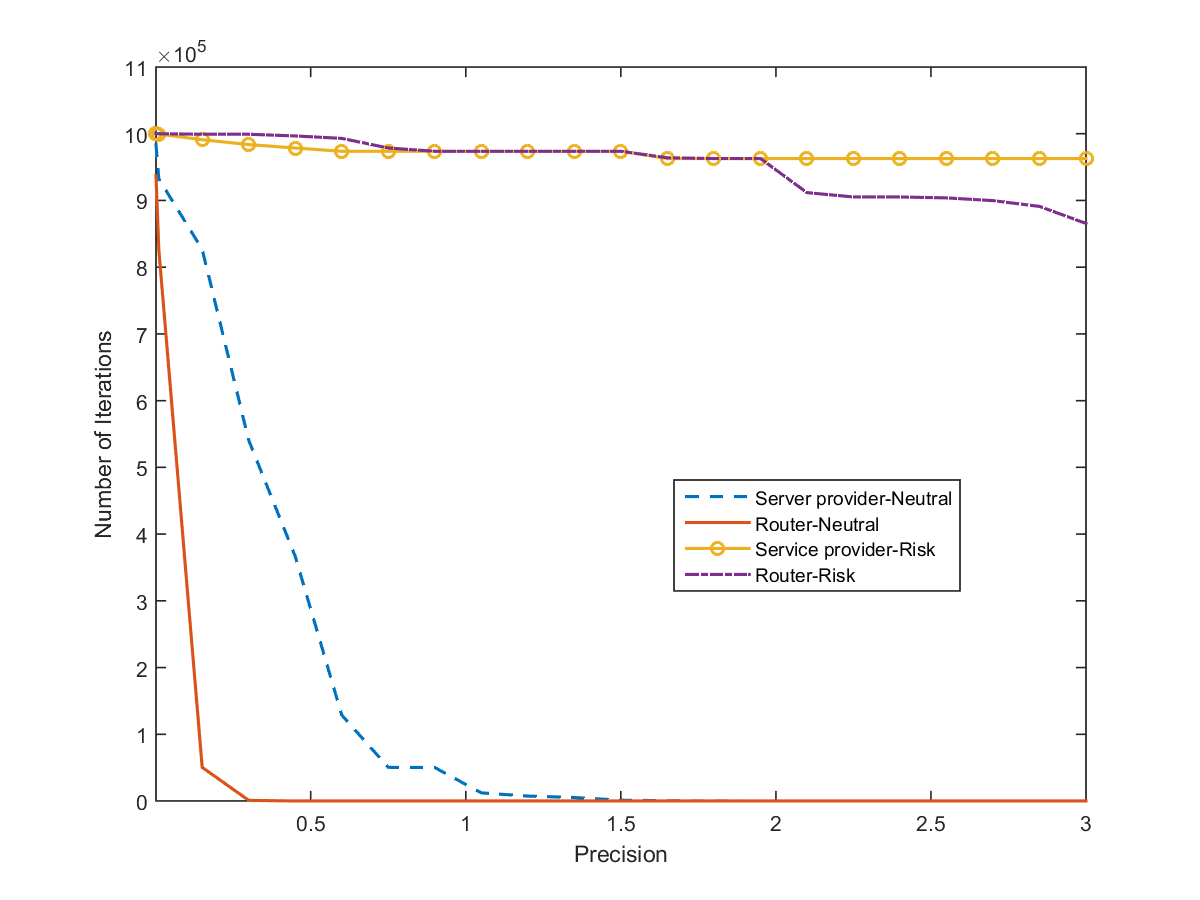
Figure 3: Comparison between NashQL and RaNashQL

Figure 2 presents the Markov perfect equilibrium for the risk-neutral and risk-aware cases. It shows the equilibrium shifting when considering the risk-awareness of players. It also shows that the both risk-neutral and risk-aware Markov perfect equilibrium are sensitive to the perturbations in the service rates, and risk-aware strategies for both players highly fluctuate with the change of state (number of packet in the queuing system). We also study how the risk tolerance level $\alpha^{i}$ (See Table 2) affects the risk-aware Markov perfect equilibrium, which also shows the risk-aware Markov perfect equilibrium fluctuates with the change of the risk tolerance level of CVaR.

	Service Provider ($\alpha^{1}$)	Router ($\alpha^{2}$)
Scenario 1	0.1	0.1
Scenario 2	0.2	0.2
Scenario 3	0.1	0.2
Scenario 4	0.2	0.1

Table 5: Risk Tolerance Level $\alpha^{i}$

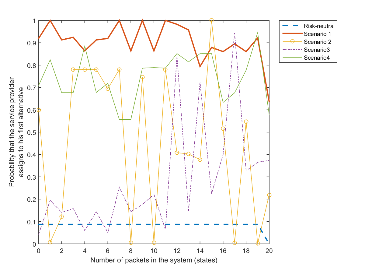
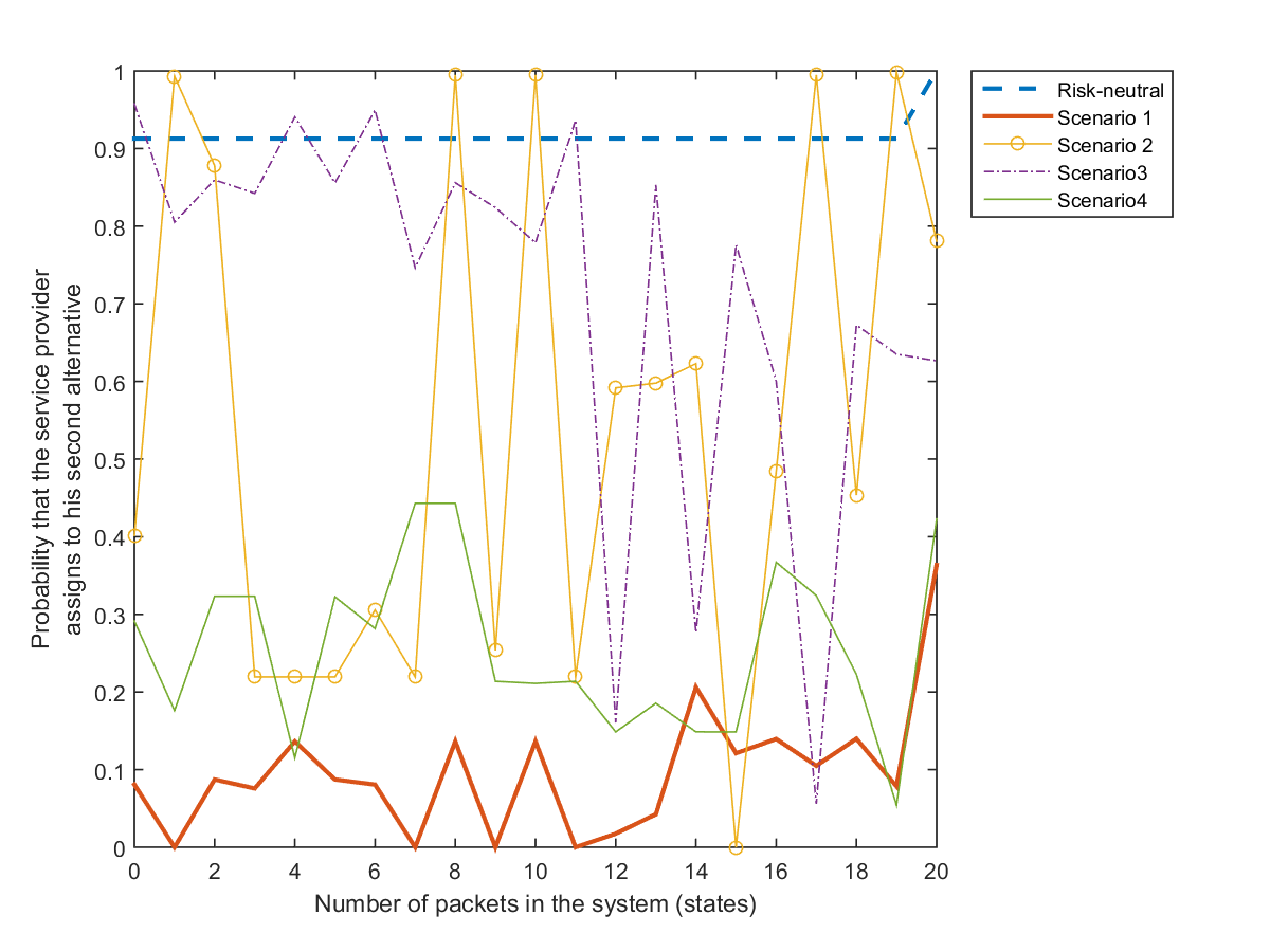
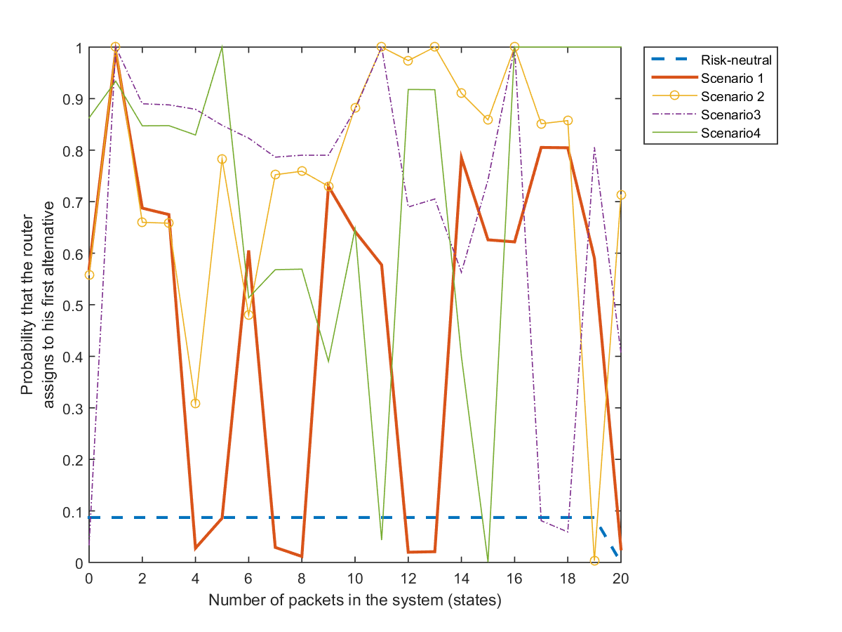
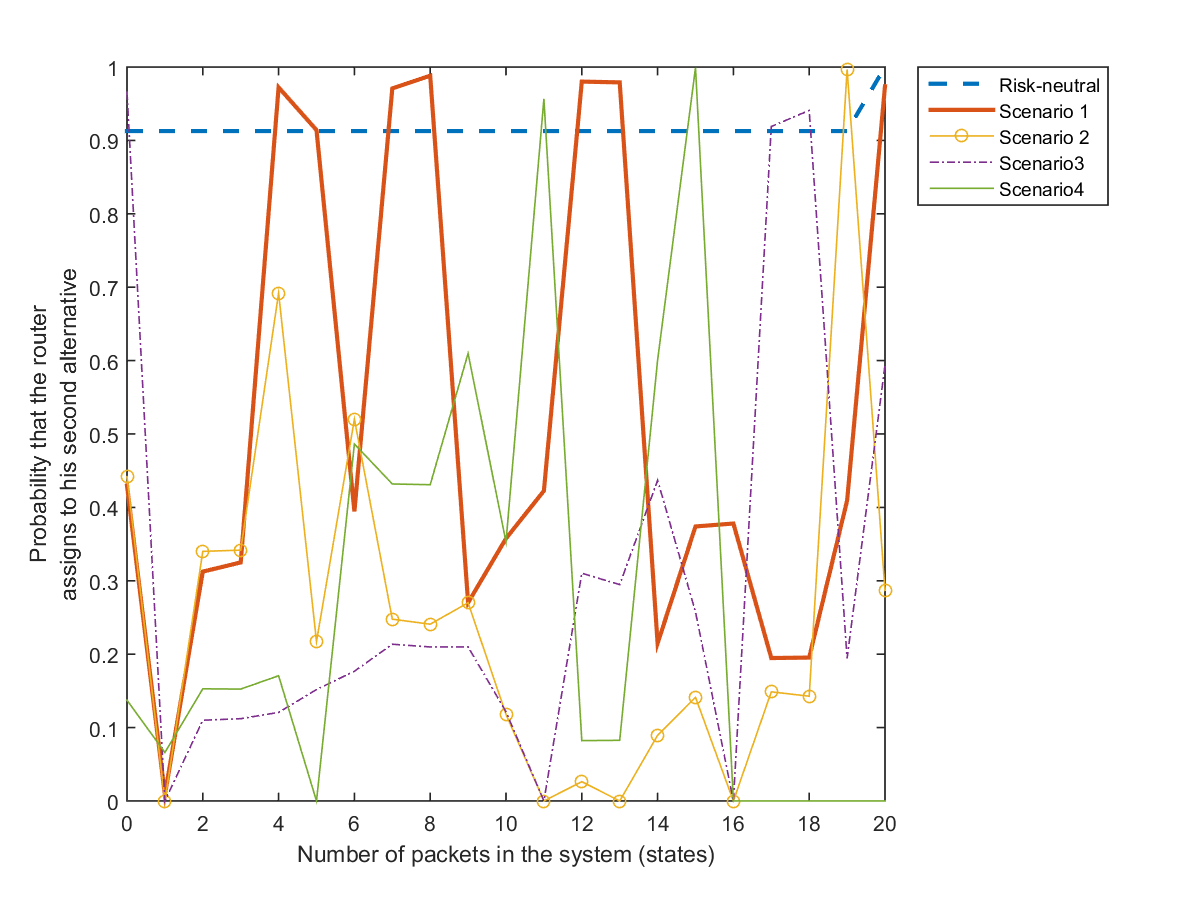
Figure 4: Comparison of Risk-Neutral and Risk-aware Markov Perfect Equilibrium

Next, we evaluate the discounted cost under risk-neutral and risk-aware Markov perfect equilibrium in simulation ($1000$ complete runs of the algorithm to compute the entire risk-aware Markov perfect equilibria). The risk tolerance levels are selected as $\alpha^{1}=\alpha^{2}=0.1$, for the risk-aware (CVaR) method in Table 3 here. Table 3 shows that considering risk awareness will significantly increase the variance of the discounted cost, which is contrary to expectation. The possible reason is the higher fluctuation of risk-aware strategies with the change of state (number of packet in the queuing system) than risk-neutral strategies.

Player	Method	Mean	Variance	$5$%-CVaR	$10$%-CVaR
Service Provider	Risk-neutral	$-22.22$	$1.4736e-06$	$-22.22$	$-22.22$
	Risk-aware (CVaR)	$-77.78$	$407.84$	$-69.34$	$-68.26$
Router	Risk-neutral	$37.48$	$7.32$	$37.94$	$38.18$
	Risk-aware (CVaR)	$83.68$	$491.20$	$86.03$	$87.54$

Table 6: Simulation for Risk-neutral Strategies and Risk-aware Strategies ($\alpha^{1}=\alpha^{2}=0.1$)

Experiment II: In this experiment, we consider a special case where the risk only comes from the stochasticity from state transitions (this setting is basically a risk-aware interpretation of [31] where the ambiguity is over the transition kernel). In this special case, we can compute risk-aware Markov equilibrium using a multilinear system as detailed in Section A.9. We evaluate performance in terms of the relative error

$$\frac{\sqrt{\sum_{s\in\mathcal{S}}\left(Nash^{i}(Q_{n,\,T}^{j}(s))_{j\in\mathcal{I}}-v_{\ast}^{i}(s)\right)^{2}}}{\sqrt{\sum_{s\in\mathcal{S}}v_{\ast}^{i}(s)^{2}}},\,n\leq N.$$

In this experiment, we take the risk measure as $10\%$-CVaR. The multilinear system is solved by an interior point algorithm within $5\times 10^{7}$ maximum function evaluation and $1\times 10^{5}$ maximum iterations, and it converges to a local optimal solution in $10471.975$ seconds. For RaNashQL, we choose $T=10$ and $N=2\times 10^{6}$, and the total implementation time for RaNashQL is $10245.314$ seconds. The following Figure 3 validates the almost sure convergence of RaNashQL to the service provider’s strategy. For the router, the relative error is large (around $190$%). One possible reason is that RaNashQL converges to different equilibria compared to the one obtained by the multilinear system solver. We see that RaNashQL possesses superior computational performance than interior point algorithm for this task, since the relative error of service provider is within $25\%$ in $1\times 10^{6}$ iterations, and the implementation time will be $5122.657$ seconds.

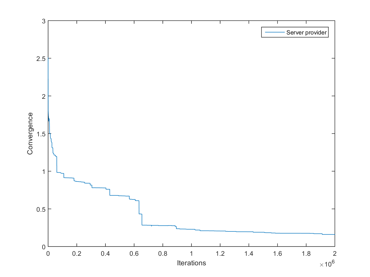
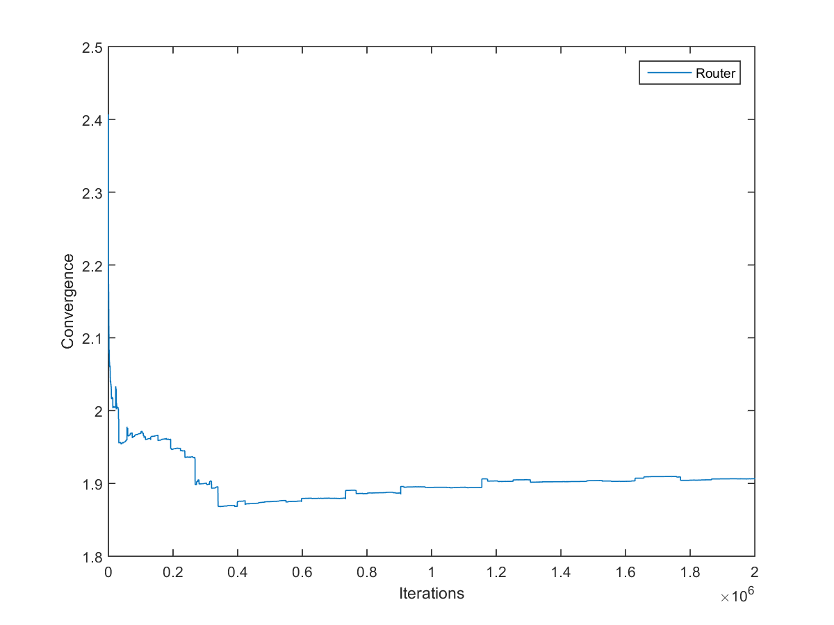
Figure 5: Almost Sure Convergence of RaNashQL

References

- [1] Michele Aghassi and Dimitris Bertsimas. Robust game theory. Mathematical Programming, 107(1-2):231–273, 2006.
- [2] Philippe Artzner, Freddy Delbaen, Jean-Marc Eber, and David Heath. Coherent measures of risk. Math. Finance, 9(3):203–228, 1999.
- [3] Arnab Basu and Mrinal K Ghosh. Nonzero-sum risk-sensitive stochastic games on a countable state space. Mathematics of Operations Research, 43(2):516–532, 2017.
- [4] Robert G. Batson. Combinatorial behavior of extreme points of perturbed polyhedra. 127:130–139, 1987.
- [5] Nicole Bäuerle and Ulrich Rieder. Zero-sum risk-sensitive stochastic games. Stochastic Processes and their Applications, 127(2):622–642, 2017.
- [6] Michael GH Bell and Chris Cassir. Risk-averse user equilibrium traffic assignment: an application of game theory. Transportation Research Part B: Methodological, 36(8):671–681, 2002.
- [7] Dimitri P Bertsekas and John N Tsitsiklis. Neuro-dynamic programming. Athena Scientific Belmont, MA, 1996.
- [8] Dimitris Bertsimas and David B. Brown. Constructing uncertainty sets for robust linear optimization. Operations Research, 57(6):1483–1495, 2009.
- [9] Vivek S Borkar et al. Stochastic approximation. Cambridge Books, 2008.
- [10] Vivek S Borkar and Sean P Meyn. The ode method for convergence of stochastic approximation and reinforcement learning. SIAM Journal on Control and Optimization, 38(2):447–469, 2000.
- [11] Leo Breiman. Probability, volume 7 of classics in applied mathematics. Society for Industrial and Applied Mathematics (SIAM), Philadelphia, PA, 1992.
- [12] Artur Czumaj, Michail Fasoulakis, and Marcin Jurdziński. Multi-player approximate nash equilibria. In Proceedings of the 16th Conference on Autonomous Agents and MultiAgent Systems, pages 1511–1513. International Foundation for Autonomous Agents and Multiagent Systems, 2017.
- [13] Ruchira S. Datta. Using computer algebra to find nash equilibria. In Proceedings of the 2003 International Symposium on Symbolic and Algebraic Computation, ISSAC ’03, pages 74–79, New York, NY, USA, 2003. ACM.
- [14] Dirk Engelmann and Jakub Steiner. The effects of risk preferences in mixed-strategy equilibria of 2 2 games. Games and Economic Behavior, 60(2):381–388, 2007.
- [15] Eyal Even-Dar and Yishay Mansour. Learning rates for q-learning. The Journal of Machine Learning Research, 5:1–25, 2004.
- [16] Michael Ferris and Andy Philpott. Dynamic risked equilibrium, 2018.
- [17] Arlington M Fink. Equilibrium in a stochastic -person game. Journal of science of the hiroshima university, series ai (mathematics), 28(1):89–93, 1964.
- [18] Hans Föllmer and Alexander Schied. Convex measures of risk and trading constraints. Finance and stochastics, 6(4):429–447, 2002.
- [19] Mrinal K Ghosh, K Suresh Kumar, and Chandan Pal. Zero-sum risk-sensitive stochastic games for continuous time markov chains. Stochastic Analysis and Applications, 34(5):835–851, 2016.
- [20] Vincent Guigues, Volker Krätschmer, and Alexander Shapiro. Statistical inference and hypotheses testing of risk averse stochastic programs. arXiv preprint arXiv:1603.07384, 2016.
- [21] Sébastien Hémon, Michel de Rougemont, and Miklos Santha. Approximate nash equilibria for multi-player games. In International Symposium on Algorithmic Game Theory, pages 267–278. Springer, 2008.
- [22] P. Jean-Jacques Herings and Ronald J. A. P. Peeters. Stationary equilibria in stochastic games: structure, selection, and computation. Journal of Economic Theory, 118:32–60, 2004.
- [23] Junling Hu and Michael P Wellman. Nash q-learning for general-sum stochastic games. Journal of machine learning research, 4(Nov):1039–1069, 2003.
- [24] Junling Hu and Michael P Wellman. Nash q-learning for general-sum stochastic games. Journal of machine learning research, 4(Nov):1039–1069, 2003.
- [25] W. Huang and W. B. Haskell. Risk-aware q-learning for Markov decision processes. In Proc. IEEE 56th Annual Conf. Decision and Control (CDC), pages 4928–4933, December 2017.
- [26] Wenjie Huang and William B Haskell. Stochastic approximation for risk-aware markov decision processes. arXiv preprint arXiv:1805.04238, 2018.
- [27] Daniel R Jiang and Warren B Powell. Risk-averse approximate dynamic programming with quantile-based risk measures. Mathematics of Operations Research, 43(2):554–579, 2017.
- [28] Victor Richmond R Jose and Jun Zhuang. Incorporating risk preferences in stochastic noncooperative games. IISE Transactions, 50(1):1–13, 2018.
- [29] Shizuo Kakutani et al. A generalization of brouwer’s fixed point theorem. Duke mathematical journal, 8(3):457–459, 1941.
- [30] Erim Kardes, Fernando Ordonez, and Randolph W. Hall. Discounted robust stochastic games and an application to queueing control. Operations Research, 59(2):365–382, 2011.
- [31] Erim Kardeş, Fernando Ordóñez, and Randolph W Hall. Discounted robust stochastic games and an application to queueing control. Operations research, 59(2):365–382, 2011.
- [32] M. B. Klompstra. Nash equilibria in risk-sensitive dynamic games. IEEE Transactions on Automatic Control, 45(7):1397–1401, July 2000.
- [33] Harold J. Kushner and G.George Yin. Stochastic Approximation and Recursive Algorithms and Applications. Springer, 2003.
- [34] Carlton E Lemke and Joseph T Howson, Jr. Equilibrium points of bimatrix games. Journal of the Society for Industrial and Applied Mathematics, 12(2):413–423, 1964.
- [35] Jonathan Levin. Choice under uncertainty. Lecture Notes, 2006.
- [36] Adam B Levy, Ren6 A Poliquin, and R Tyrrell Rockafellar. Stability of locally optimal solutions. SIAM Journal on Optimization, 10(2):580–604, 2000.
- [37] Michael L Littman, Nishkam Ravi, Arjun Talwar, and Martin Zinkevich. An efficient optimal-equilibrium algorithm for two-player game trees. arXiv preprint arXiv:1206.6855, 2012.
- [38] Richard D McKelvey and Andrew McLennan. Computation of equilibria in finite games. Handbook of computational economics, 1:87–142, 1996.
- [39] Karthik Natarajan, Dessislava Pachamanova, and Melvyn Sim. Constructing risk measures from uncertainty sets. Oper. Res., 57:1129–1141, September 2009.
- [40] Arkadi Nemirovski and Reuven Rubinstein. An efficient stochastic approximation algorithm for stochastic saddle point problems. Modeling Uncertainty, pages 156–184, 2005.
- [41] Jean-Paul Penot. On the convergence of subdifferentials of convex functions. Nonlinear Analysis: Theory, Methods & Applications, 21(2):87–101, 1993.
- [42] Krzysztof Postek, Dick Den Hertog, and Bertrand Melenberg. Computationally tractable counterparts of distributionally robust constraints on risk measures. 2015.
- [43] Yundi Qian, William B Haskell, and Milind Tambe. Robust strategy against unknown risk-averse attackers in security games. In Proceedings of the 2015 International Conference on Autonomous Agents and Multiagent Systems, pages 1341–1349. International Foundation for Autonomous Agents and Multiagent Systems, 2015.
- [44] Andrzej Ruszczyński. Risk-averse dynamic programming for markov decision processes. Mathematical programming, 125(2):235–261, 2010.
- [45] Andrzej Ruszczynski and Alexander Shapiro. Optimization of convex risk functions. Mathematics of operations research, 31(3):433–452, 2006.
- [46] Andrzej Ruszczyński and Alexander Shapiro. Optimization of convex risk functions. Mathematics of operations research, 31(3):433–452, 2006.
- [47] Alexander Shapiro and Alois Pichler. Time and dynamic consistency of risk averse stochastic programs. optimization-online.org, 2016.
- [48] Yun Shen, Wilhelm Stannat, and Klaus Obermayer. Risk-sensitive markov control processes. SIAM Journal on Control and Optimization, 51(5):3652–3672, 2013.
- [49] Csaba Szepesvári and Michael L Littman. A unified analysis of value-function-based reinforcement-learning algorithms. Neural computation, 11(8):2017–2060, 1999.
- [50] Yasushi Terazono and Ayumu Matani. Continuity of optimal solution functions and their conditions on objective functions. SIAM Journal on Optimization, 25(4):2050–2060, 2015.
- [51] PJ Thomas. Measuring risk-aversion: The challenge. Measurement, 79:285–301, 2016.
- [52] John von Neumann and Oskar Morgenstern. Theory of Games and Economic Behavior. Princeton University Press, 1944.
- [53] OJ Vrieze. Stochastic games and stationary strategies. In Stochastic Games and Applications, pages 37–50. Springer, 2003.
- [54] David W Walkup and Roger J-B Wets. A lipschitzian characterization of convex polyhedra. Proceedings of the American Mathematical Society, pages 167–173, 1969.
- [55] Pengqian Yu, William B Haskell, and Huan Xu. Approximate value iteration for risk-aware markov decision processes. IEEE Transactions on Automatic Control, 2018.