Soil Texture Classification with 1D Convolutional Neural Networks based on Hyperspectral Data

Abstract

Soil texture is important for many environmental processes. In this paper, we study the classification of soil texture based on hyperspectral data. We develop and implement three 1-dimensional (1D) convolutional neural networks (CNN): the LucasCNN, the LucasResNet which contains an identity block as residual network, and the LucasCoordConv with an additional coordinates layer. Furthermore, we modify two existing 1D CNN approaches for the presented classification task. The code of all five CNN approaches is available on GitHub (Riese,, 2019). We evaluate the performance of the CNN approaches and compare them to a random forest classifier. Thereby, we rely on the freely available LUCAS topsoil dataset. The CNN approach with the least depth turns out to be the best performing classifier. The LucasCoordConv achieves the best performance regarding the average accuracy. In future work, we can further enhance the introduced LucasCNN, LucasResNet and LucasCoordConv and include additional variables of the rich LUCAS dataset.

1 INTRODUCTION

The texture of soil influences the soil’s capability to store water and its fertility. Therefore, the classification of soil texture is important for agricultural applications as well as for the monitoring of environmental processes. The term soil texture refers to the relative content of soil particles of various sizes. It is determined by the percentages of clay, sand and silt in the soil. Soil texture can be classified with respect to these three properties e.g. according to the KA5 taxonomy defined by Eckelmann et al., (2006).

The monitoring of soil texture with in-situ measurements is expensive and is not feasible on large areas. To cover such large areas, optical remote sensing provides a good alternative. For example, hyperspectral sensors are such optical remote sensing devices which measure solar reflectance spectra of objects. The information of soil texture derived from the soil reflectance corresponds to specific absorption features of clay or other soil mineral and organic constituents (Cloutis,, 1996). For a classification of soil texture based on hyperspectral data, a model has to be developed that is able to link different reflectance spectra to the respective soil textures.

The field of machine learning provides well-suited techniques to learn the links between the hyperspectral data and soil texture. Machine learning techniques can be divided into shallow learning and deep learning approaches. Shallow learning approaches like support vector machines (Vapnik,, 1995), random forest (Breiman,, 2001; Geurts et al.,, 2006) and self-organizing maps (Kohonen,, 1990) have shown good performance in the past with hyperspectral estimation tasks (Melgani and Bruzzone,, 2004; Ham et al.,, 2005; Riese and Keller,, 2018). Recent studies focus on deep learning approaches, meaning network architectures with several hidden layers. One subcategory of deep neural networks are convolutional neural networks (CNN). In contrast to common fully-connected neural networks, the number of trainable parameters of CNNs are independent of the size of the input data. This makes CNNs interesting candidates for the classification of high-dimensional data like hyperspectral data.

In this paper, we use the freely available Land Use/Cover Area Frame Statistical Survey (LUCAS) Soil dataset. It includes hyperspectral and soil texture data from measurements all over Europe. Based on this dataset, we assess the performance of several CNN models with respect to the classification of soil texture. Our main contributions are:

• the pre-processing of the freely available LUCAS soil dataset,

• the modification of two existing CNN approaches to the classification task,

• the development and implementation of three own CNN approaches including a residual network and a CNN with an extra coordinates layer and

• a comprehensive evaluation of all applied approaches.

We give an overview of the current research in hyperspectral classification and soil texture classification in Section 2. The dataset and its pre-processing is described in Section 3. The applied machine learning approaches are introduced in Section 4. Section 5 contains the evaluation of the different approaches. Finally, we conclude this study and give an outlook of possible future research ideas in Section 6.

2 Related Work

In this section, we briefly review the published research which is related to the presented classification of soil texture based on hyperspectral data. A first review of geological remote sensing is given by Cloutis, (1996). Traditional approaches like nearest mean, nearest neighbor, maximum likelihood, hidden Markov models and spectral angle matching for the classification of soil texture show acceptable results (Zhang et al.,, 2003, 2005; Shrestha et al.,, 2005).

The increasing popularity of deep learning approaches in many research disciplines has also reached the field of remote sensing. Deep learning approaches turn out to solve classification tasks better than shallow methods (Hinton and Salakhutdinov,, 2006). Zhu et al., (2017) give a detailed overview of deep learning in remote sensing and Petersson et al., (2016) review the application of deep learning in hyperspectral image analysis. The application of 2-dimensional CNNs for classification and regression tasks based on hyperspectral images is proposed among others by Makantasis et al., (2015). The two dimensions refer to the two spatial dimensions of hyperspectral images. Since hyperspectral images consist of several spectral channels, one additional dimension is possible: the spectral dimension. This spectral dimension can be utilized as a third dimension of a CNN or can be analyzed on its own by 1-dimensional (1D) CNNs. Hu et al., (2015) propose the use of 1D CNNs based on the spectral dimension of hyperspectral images. This network is described in Section 4 in detail.

In most publications, the applied machine learning approaches are trained on a specific training dataset. Zhao et al., (2017) propose the use of pre-trained networks for the hyperspectral image classification, so called transfer learning. In transfer learning, it is assumed that the trained features of a neural network are comparable between different image datasets. Therefore, this approach is time-saving and enables training on smaller datasets. The latter is possible since the training of the neural network is mostly done with another dataset beforehand (pre-trained). Transfer learning of a 1D CNN is proposed by Liu et al., 2018a . They apply the CNN for the regression of clay content in the soil based on the LUCAS soil dataset. We describe this approach in detail in Section 4 and compare it to other methods with respect to our classification task.

3 Dataset

In the following Section 3.1, the dataset used in this study is described. The pre-processing of this dataset is summarized in Section 3.2.

3.1 The LUCAS dataset

The Land Use/Cover Area Frame Statistical Survey (LUCAS) Soil dataset is a large and comprehensive survey of topsoil (Tóth et al., 2013b, ; Tóth et al., 2013a, ; Orgiazzi et al.,, 2018). The dataset was collected in different locations all over Europe between 2009 and 2012. Further measurements have been performed in 2018 but are not included into this publication. The LUCAS dataset consists of about $22\,000$ datapoints that include physico-chemical properties like the percentage of coarse fragments, the particle size distributions clay, sand and silt, the pH value, the organic carbon content, the carbonate content, the total nitrogen content, the extractable potassium content, the phosphorus content, the cation exchange capacity and metals. Additionally, this dataset includes continuous reflectance spectra from $400\text{\,}\mathrm{nm}2500\text{\,}\mathrm{nm}$, referred to as hyperspectral data in the following. The spectral resolution of the applied sensor is $0.5\text{\,}\mathrm{nm}$. The new 2018 dataset will include, among others, soil biodiversity properties and soil moisture data (Orgiazzi et al.,, 2018).

Based on the LUCAS dataset, a variety of studies exists. For example, the estimation of $\mathrm{N_{2}O}$ is shown by Lugato et al., (2017). Several studies focus on the soil organic carbon content (Panagos et al.,, 2013; Nocita et al.,, 2014; Castaldi et al.,, 2018). Studies about land cover and land use diversity benefit from the large area covered by the LUCAS dataset. They calculate landscape indices (Palmieri et al., 2011a, ; Palmieri et al., 2011b, ) and combine land use data with Landsat images (Pflugmacher et al.,, 2019). The soil erodibility is studied by Panagos et al., (2014).

As stated in Section 2, the soil texture information is addressed in several studies applying machine learning techniques. For example, Ballabio et al., (2016) perform a regression of soil properties such as the three layers of soil texture (clay, sand, silt) plus coarse fragments with the MARS model. A recent study applies 1D CNNs to estimate the clay content (Liu et al., 2018a, ).

3.2 Pre-processing

In this paper, we rely on the LUCAS dataset which was processed beforehand according to Tóth et al., 2013a . In addition, we apply three pre-processing steps as illustrated in Figure 1 in the following order:

1. Dimensionality reduction to reduce the number of spectral bands of the hyperspectral data from $4200$ to $256$ with minimal information loss by averaging $16\text{\,}17\text{\,}$ neighboring bands to one new band. This dimensionality reduction is necessary for practical reasons, e.g. to reduce the computation time and to avoid overtraining by minimizing the weights of the networks.

2. Removal of the duplicates of the multiple hyperspectral datapoints per soil sample and removal of unused features to generate a minimal classification dataset. This step reduces the bias of the training and evaluation of machine learning techniques.

3. Aggregation the general soil classes L, S, T, U for the supervised classification performed below.

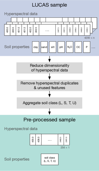
Figure 1: Preprocessing workflow with three steps: the dimensionality reduction, the removal of the duplicates and the aggregation of the general soil classes.

We rely on the main group soil classes according to Eckelmann et al., (2006) consisting of the classes L (loam), S (sand), T (clay) and U (silt). The class names are derived from the German words ”Lehm”, ”Sand”, ”Ton” and ”Schluff”. The classification is based on the distribution of clay, sand and silt contents. The distribution of the datapoints based on these soil classes is shown in Figure 2.

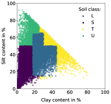
Figure 2: Clay and silt content of all pre-processed datapoints of the LUCAS dataset. The color of the datapoints symbolizes the respective soil class introduced in this paper.

To evaluate the performance of the different classification approaches, the pre-processed dataset is split into three disjoint subsets: the training subset, the validation subset and the test subset. We choose random splitting with a ratio of approximately $60:20:20$. In total, the training subset consists of $9759$ datapoints, the validation subset contains $3109$ datapoints and the test subset contains $3208$ datapoints. The class distributions of the three datasets are shown in Figure 3. One datapoint consists of $256$ hyperspectral reflectance values and one of the four soil classes L, S, T, U.

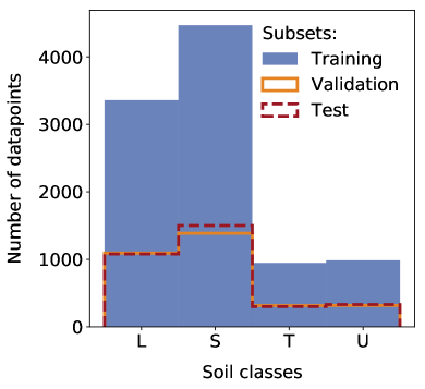
Figure 3: Class distributions of the three datasets: training, validation and test.

4 Methodology

For supervised learning based on hyperspectral images, various methods exist. For example, Keller et al., 2018a ; Keller et al., 2018b combine ten shallow learning techniques for the regression of environmental variables. For the presented soil texture classification task, we study several machine learning approaches. All approaches are CNNs except for the random forest (RF) classifier. The RF classifier is established in remote sensing applications (see e.g. Ham et al., (2005)). Therefore, the classification accuracy of the several CNN approaches is compared against the results of the RF classifier.

In addition to the RF classifier, we study five different 1D CNN architectures. Two of them have been introduced by Hu et al., (2015) and Liu et al., 2018a and are modified for the underlying classification task. The 1D CNN of Hu et al., (2015) consists of one 1D convolutional layer followed by one max-pooling layer and one fully-connected (FC) layer. The 1D CNN of Liu et al., 2018a was introduced as a regression approach for the estimation of clay content based on the LUCAS dataset. It consists of four 1D convolutional layers each followed by a max-pooling layer. At the end of each network by Hu et al., (2015) and Liu et al., 2018a , we implement one FC layer with a softmax activation and four outputs. This prepares these CNNs for the classification task of this study.

In addition to these two existing CNN approaches, we introduce three 1D CNN architectures for the soil texture classification. All three architectures are inspired by the LeNet5 network (Lecun et al.,, 1998). In order to distinguish between the three implemented CNNs, we refer to the three architectures as LucasCNN, LucasResNet and LucasCoordConv. In Figure 4, the architectures of the three Lucas networks are illustrated. The LucasCNN consists of four convolutional layers, each followed by a max-pooling layer with a kernel size of $2$. After flattening the output of the fourth convolutional layer, two FC layers are implemented and, as before, one FC layer with a softmax activation and four outputs is placed at the end of the network.

For the LucasResNet, we add an identity block to the LucasCNN. The input vector is bypassing the four convolutional layer and is concatenated to the activation of the last convolutional layer and before the first FC layers. The special feature of the LucasCoordConv is one coordinates layer placed before the first convolutional layer of the LucasCNN. Liu et al., 2018b introduced such a coordinates layer first. The network architecture after the first convolutional layer remains the same as in the LucasCNN. The code of all presented implementations of 1D CNNs is published on GitHub (Riese,, 2019).

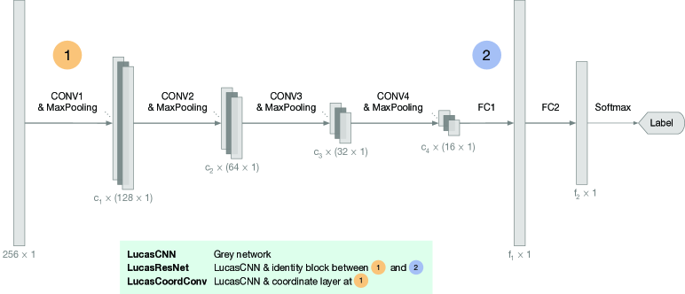
Figure 4: Flowchart of the LucasCNN (grey). The network consist of convolutional (CONV), fully-connected (FC) layers and max-pooling layers. The $i$-th CONV layer consists of $c_{i}$ filters and the $j$-th FC layer consists of $f_{j}$ units. For the LucasResNet, an identity block is implemented between the marker 1 and 2. For the LucasCoordConv, a coordinates layer is inserted before the first CONV layer at marker 1. At the end of each network, a softmax layer provides the classification output as a 4-dimensional vector.

5 Results and discussion

The classification results are compared based on the overall accuracy (OA), average accuracy (AA) and Cohen’s kappa coefficient $\kappa$. The OA is defined as number of correctly classified datapoints divided by the size of the dataset. The AA is the sum of the recall of each class divided by the number of classes. The recall of a class is defined as the number of correctly classified instances (datapoints) of that class, divided by the total number of instances of that class. Finally, $\kappa$ is defined as

$$\kappa=\frac{\mathrm{OA}-\theta}{1-\theta},$$ (1)

with the hypothetical probability of chance agreement $\theta$.

Machine learning models are characterized by two types of parameters: model parameters and hyperparameters. Model parameters are adapted during the training of the model and hyperparameters are set beforehand. For the RF classifier, we use the implementation of Pedregosa et al., (2011) with $10\,000$ estimators. This configuration achieves good results e.g. in a regression task based on hyperspectral data (Keller et al., 2018b, ). All hyperparameters of the two existing CNNs are adopted from the respective introducing publications. The hyperparameters of the three new approaches LucasCNN, LucasResNet and LucasCoordConv are determined with a hyperparameter optimization process.

The training dataset is used for the training of each CNN while their evaluation is performed on the validation dataset. The hyperparameters of the all five 1D CNN approaches are shown in Table 1. The test dataset is not used for this procedure.

Table 1: Hyperparameters of the new 1D CNN approaches LucasCNN, LucasResNet and LucasCoordConv as well as the existing CNN approaches by Hu et al., (2015) and Liu et al., 2018a . The number of filters in the $i$-th CONV layer is defined as $c_{i}$ and the number of units in the $i$-th FC layer is defined as $f_{j}$.

Hyperparameters	LucasCNN	LucasResNet	LucasCoordConv	Hu et al., (2015)	Liu et al., 2018a
Number of epochs	150	120	120	200	235
Batch size	100	64	32	100	100
Kernel size	3	3	3	28	3
Pooling size	2	2	2	6	2
Activations	ReLU	ReLU	ReLU	$\tanh$	ReLU
Padding	valid	same	valid	valid	valid
$c_{1}$	32	32	32	20	32
$c_{2}$	32	32	64	-	32
$c_{3}$	64	64	64	-	64
$c_{4}$	64	64	128	-	64
$f_{1}$	120	150	256	100	-
$f_{2}$	160	100	128	-	-
Loss	categorical crossentropy
Optimizer	Adam

Based on the test dataset, the final classification results are calculated (see Table 2). The RF classifier shows the worst performance. The classifier based on the CNN by Hu et al., (2015) achieves the best performance with respect to OA and $\kappa$. It represents the most basic CNN implementation in this study. This directly implies that smaller networks with larger kernel sizes (28 vs. 3) solve the presented classification task. Another finding is that adding the identity block in the LucasResNet and the coordinates layer in the LucasCoordConv slightly improves the performance of the network compared to the LucasCNN. Moreover, the added coordinates layer in the LucasCoordConv improves the AA significantly. Therefore, the LucasCoordConv represents the best approach of this study with respect to this performance metric.

Table 2: Classification results based on the test subset.

Model	OA	AA	$\kappa$
Random forest	$0.63$	$0.47$	$0.41$
Liu et al., 2018a	$0.70$	$0.59$	$0.54$
Hu et al., (2015)	$0.74$	$0.61$	$0.59$
LucasCNN	$0.71$	$0.56$	$0.54$
LucasResNet	$0.72$	$0.56$	$0.55$
LucasCoordConv	$0.73$	$0.62$	$0.57$

Beyond that, the impact of the coordinates layer is shown in the confusion matrices in Figure 5. In general, the classes L and S are correctly classified in more than $70\text{\,}\mathrm{\char 37\relax}$ of the cases. In contrast, the class U and especially the class T are misclassified. Two findings can be derived from this result: first, the class T is more difficult to distinguish from the other classes based on hyperspectral data. Second, adding a coordinates layer in the LucasCoordConv improves the classification performance significantly. While all other classifiers label more than $70\text{\,}\mathrm{\char 37\relax}$ of the class T as class L, the LucasCoordConv only misclassifies about $48\text{\,}\mathrm{\char 37\relax}$ as class L.

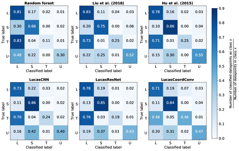
Figure 5: Normalized confusion matrices based on the test dataset.

6 Conclusion

In this paper, we address the classification of soil texture based on hyperspectral data with 1D CNNs. We use the freely available LUCAS soil dataset and describe its pre-processing and splitting in detail. For the classification of the dataset, we apply a RF classifier as well as two existing 1D CNNs by Hu et al., (2015) and Liu et al., 2018a . In addition, we introduce three new approaches LucasCNN, LucasResNet and LucasCoordConv.

After the hyperparameter optimization of the three new approaches, we compare the classification performance of all six approaches based on the metrics OA, AA and $\kappa$ as well as the confusion matrices. We conclude, that the RF classifier is incapable of handling this classification task sufficiently. All five CNN approaches show similar classification results. The most basic CNN approach by Hu et al., (2015) achieves the best performance in OA and $\kappa$. The introduced LucasCoordConv, which includes a coordinates layer according to Liu et al., 2018b , performs best regarding the AA. This means that this approach performs best on each individual class.

This study presents a further step towards the classification of hyperspectral data based on CNNs. Although up to now, 1D CNNs are often underrated in context of hyperspectral classification tasks, we demonstrate their potential on the LUCAS dataset. In general, the application of 2D and 3D CNNs on point measurements as the LUCAS dataset is not possible by definition. However, the results of this publication can be of value for studies focussing methodologically on 3D CNNs utilizing the spectral dimension as third dimension, e.g. Chen et al., (2016). In future work, we can further enhance the introduced LucasCNN, LucasResNet and LucasCoordConv and include additional variables of the rich LUCAS dataset. Regularization methods like dropout and batch normalization can help to generalize the presented CNN approaches. Additionally, techniques like transfer learning with 1D CNNs and their applications on new datasets like the LUCAS 2018 (Orgiazzi et al.,, 2018) dataset are promising. Furthermore, the developed methods of this publication can be applied on upcoming hyperspectral satellite data like EnMAP.

References

- Ballabio et al., (2016) Ballabio, C., Panagos, P. and Monatanarella, L., 2016. Mapping topsoil physical properties at European scale using the LUCAS database. Geoderma 261, pp. 110–123.
- Breiman, (2001) Breiman, L., 2001. Random forests. Machine Learning 45(1), pp. 5–32.
- Castaldi et al., (2018) Castaldi, F., Chabrillat, S., Jones, A., Vreys, K., Bomans, B. and Wesemael, B. v., 2018. Soil organic carbon estimation in croplands by hyperspectral remote apex data using the lucas topsoil database. Remote Sensing 10(2), pp. 153.
- Chen et al., (2016) Chen, Y., Jiang, H., Li, C., Jia, X. and Ghamisi, P., 2016. Deep feature extraction and classification of hyperspectral images based on convolutional neural networks. IEEE Transactions on Geoscience and Remote Sensing 54(10), pp. 6232–6251.
- Cloutis, (1996) Cloutis, E. A., 1996. Review article hyperspectral geological remote sensing: evaluation of analytical techniques. International Journal of Remote Sensing 17(12), pp. 2215–2242.
- Eckelmann et al., (2006) Eckelmann, W., Sponagel, H., Grottenthaler, W., Hartmann, K.-J., Hartwich, R., Janetzko, P., Joisten, H., Kühn, D., Sabel, K.-J. and Traidl, R., 2006. Bodenkundliche Kartieranleitung. KA5. 5 edn, Schweizerbart’sche Verlagsbuchhandlung.
- Geurts et al., (2006) Geurts, P., Ernst, D. and Wehenkel, L., 2006. Extremely randomized trees. Machine Learning 63(1), pp. 3–42.
- Ham et al., (2005) Ham, J., Chen, Y., Crawford, M. M. and Ghosh, J., 2005. Investigation of the Random Forest Framework for Classification of Hyperspectral Data. IEEE Transactions on Geoscience and Remote Sensing 43, pp. 492–501.
- Hinton and Salakhutdinov, (2006) Hinton, G. E. and Salakhutdinov, R. R., 2006. Reducing the Dimensionality of Data with Neural Networks. Science 313, pp. 504–507.
- Hu et al., (2015) Hu, W., Huang, Y., Wei, L., Zhang, F. and Li, H., 2015. Deep convolutional neural networks for hyperspectral image classification. Journal of Sensors 2015, pp. 1–12.
- (11) Keller, S., Maier, P. M., Riese, F. M., Norra, S., Holbach, A., Börsig, N., Wilhelms, A., Moldaenke, C., Zaake, A. and Hinz, S., 2018a. Hyperspectral data and machine learning for estimating cdom, chlorophyll a, diatoms, green algae, and turbidity. International Journal of Environmental Research and Public Health 15(9), pp. 1881.
- (12) Keller, S., Riese, F. M., Stötzer, J., Maier, P. M. and Hinz, S., 2018b. Developing a machine learning framework for estimating soil moisture with VNIR hyperspectral data. ISPRS Annals of Photogrammetry, Remote Sensing and Spatial Information Sciences IV-1, pp. 101–108.
- Kohonen, (1990) Kohonen, T., 1990. The self-organizing map. 78(9), pp. 1464––1480.
- Lecun et al., (1998) Lecun, Y., Bottou, L., Bengio, Y. and Haffner, P., 1998. Gradient-based learning applied to document recognition. Proceedings of the IEEE 86(11), pp. 2278–2324.
- (15) Liu, L., Ji, M. and Buchroithner, M., 2018a. Transfer learning for soil spectroscopy based on convolutional neural networks and its application in soil clay content mapping using hyperspectral imagery. Sensors 18(9), pp. 3169.
- (16) Liu, R., Lehman, J., Molino, P., Petroski Such, F., Frank, E., Sergeev, A. and Yosinski, J., 2018b. An intriguing failing of convolutional neural networks and the CoordConv solution. In: S. Bengio, H. Wallach, H. Larochelle, K. Grauman, N. Cesa-Bianchi and R. Garnett (eds), Advances in Neural Information Processing Systems 31, Curran Associates, Inc., pp. 9628–9639.
- Lugato et al., (2017) Lugato, E., Paniagua, L., Jones, A., Vries, W. d. and Leip, A., 2017. Complementing the topsoil information of the Land Use/Land Cover Area Frame Survey (LUCAS) with modelled N2O emissions. PLOS ONE 12(4), pp. 1–16.
- Makantasis et al., (2015) Makantasis, K., Karantzalos, K., Doulamis, A. and Doulamis, N., 2015. Deep Supervised Learning for Hyperspectral Data Classification Through Convolutional Neural Networks. In: 2015 IEEE International Geoscience and Remote Sensing Symposium (IGARSS), pp. 4959–4962.
- Melgani and Bruzzone, (2004) Melgani, F. and Bruzzone, L., 2004. Classification of Hyperspectral Remote Sensing Images With Support Vector Machines. IEEE Transactions on Geoscience and Remote Sensing 42, pp. 1778–1790.
- Nocita et al., (2014) Nocita, M., Stevens, A., Toth, G., Panagos, P., Wesemael, B. v. and Montanarella, L., 2014. Prediction of soil organic carbon content by diffuse reflectance spectroscopy using a local partial least square regression approach. Soil Biology and Biochemistry 68, pp. 337–347.
- Orgiazzi et al., (2018) Orgiazzi, A., Ballabio, C., Panagos, P., Jones, A. and Fernández-Ugalde, O., 2018. LUCAS Soil, the largest expandable soil dataset for Europe: a review. European Journal of Soil Science 69(1), pp. 140–153.
- (22) Palmieri, A., Dominici, P., Kasanko, M. and Martino, L., 2011a. Diversified landscape structure in the EU Member States. Statistics in focus.
- (23) Palmieri, A., Martino, L., Dominici, P. and Kasanko, M., 2011b. Land Cover and Land Use Diversity Indicators in LUCAS 2009 data. Land Quality and Land Use Information in the European Union pp. 59––68.
- Panagos et al., (2013) Panagos, P., Ballabio, C., Yigini, Y. and Dunbar, M. B., 2013. Estimating the soil organic carbon content for European NUTS2 regions based on LUCAS data collection. Science of The Total Environment 442, pp. 235–246.
- Panagos et al., (2014) Panagos, P., Meusburger, K., Ballabio, C., Borrelli, P. and Alewell, C., 2014. Soil erodibility in Europe: A high-resolution dataset based on LUCAS. Science of The Total Environment 479, pp. 189–200.
- Pedregosa et al., (2011) Pedregosa, F., Varoquaux, G., Gramfort, A., Michel, V., Thirion, B., Grisel, O., Blondel, M., Louppe, G., Prettenhofer, P., Weiss, R., Dubourg, V., Vanderplas, J., Passos, A., Cournapeau, D., Brucher, M., Perrot, M. and Duchesnay, E., 2011. Scikit-learn: Machine learning in python. Journal of Machine Learning Research 12, pp. 2825–2830.
- Petersson et al., (2016) Petersson, H., Gustafsson, D. and Bergström, D., 2016. Hyperspectral Image Analysis Using Deep Learning - A Review. 2016 Sixth International Conference on Image Processing Theory, Tools and Applications (IPTA).
- Pflugmacher et al., (2019) Pflugmacher, D., Rabe, A., Peters, M. and Hostert, P., 2019. Mapping pan-european land cover using landsat spectral-temporal metrics and the european lucas survey. Remote Sensing of Environment 221, pp. 583–595.
- Riese, (2019) Riese, F. M., 2019. CNN Soil Texture Classification. doi.org/10.5281/zenodo.2540718. Code implementation in Python.
- Riese and Keller, (2018) Riese, F. M. and Keller, S., 2018. Introducing a Framework of Self-Organizing Maps for Regression of Soil Moisture with Hyperspectral Data. In: IGARSS 2018 - 2018 IEEE International Geoscience and Remote Sensing Symposium, Valencia, Spain, pp. 6151–6154.
- Shrestha et al., (2005) Shrestha, D., Margate, D., Meer, F. v. d. and Anh, H., 2005. Analysis and classification of hyperspectral data for mapping land degradation: An application in southern spain. International Journal of Applied Earth Observation and Geoinformation 7(2), pp. 85–96.
- (32) Tóth, G., Jones, A. and Montanarella, L., 2013a. LUCAS Topsoil Survey: Methodology, Data, and Results.
- (33) Tóth, G., Jones, A. and Montanarella, L., 2013b. The LUCAS topsoil database and derived information on the regional variability of cropland topsoil properties in the European Union. Environmental Monitoring and Assessment.
- Vapnik, (1995) Vapnik, V. N., 1995. The Nature of Statistical Learning Theory. Springer-Verlag New York, Inc., New York, NY, USA.
- Zhang et al., (2003) Zhang, X., Vijayaraj, V. and Younan, N. H., 2003. Hyperspectral soil texture classification. In: IEEE Workshop on Advances in Techniques for Analysis of Remotely Sensed Data, 2003, pp. 182–186.
- Zhang et al., (2005) Zhang, X., Younan, N. H. and O’Hara, C. G., 2005. Wavelet domain statistical hyperspectral soil texture classification. IEEE Transactions on Geoscience and Remote Sensing 43(3), pp. 615–618.
- Zhao et al., (2017) Zhao, B., Huang, B. and Zhong, Y., 2017. Transfer learning with fully pretrained deep convolution networks for land-use classification. IEEE Geoscience and Remote Sensing Letters 14(9), pp. 1436–1440.
- Zhu et al., (2017) Zhu, X. X., Tuia, D., Mou, L., Xia, G., Zhang, L., Xu, F. and Fraundorfer, F., 2017. Deep learning in remote sensing: A comprehensive review and list of resources. IEEE Geoscience and Remote Sensing Magazine 5(4), pp. 8–36.