Hysteretic behavior of spatially coupled phase-oscillators

Abstract.

Motivated by phenomena related to biological systems such as the synchronously flashing swarms of fireflies, we investigate a network of phase oscillators evolving under the generalized Kuramoto model with inertia. A distance-dependent, spatial coupling between the oscillators is considered. Zeroth and first order kernel functions with finite kernel radii were chosen to investigate the effect of local interactions. The hysteretic dynamics of the synchronization depending on the coupling parameter was analyzed for different kernel radii. Numerical investigations demonstrate that (1) locally locked clusters develop for small coupling strength values, (2) the hysteretic behavior vanishes for small kernel radii, (3) the ratio of the kernel radius and the maximal distance between the oscillators characterizes the behavior of the network.

1. Introduction

Synchronization is a collective behavior observed in many fields. It is a result of the interaction between oscillators capable of adjusting their rhythms/natural frequencies. To model synchronization of coupled phase oscillators the Kuramoto model proposed in 1975 [1] is often used, for example, to investigate the collective behavior of lasers [2], neurons [3, 4, 5], social groups [6] and even crickets [7]. This model was also used to describe the interesting phenomena related to Pteroptyx malaccae, a species of firefly capable of synchronous firing with almost no phase lag [8]. This can be attributed to this insect’s ability to alter its flashing frequency in response to external stimulus [9]. Motivated by behavior of fireflies, the original first order Kuramoto model was later extended with an inertial term by Tanaka et al. [10] which allows for the adaptation of the flashing frequency of one firefly. They showed that in a fully coupled system, the degree of synchrony depends on the coupling strength between the oscillators in a hysteretic manner. The critical coupling strength necessary for the system to transition from the incoherent state to the coherent state is larger than the critical coupling strength resulting in the breaking of synchrony. According to Tanaka et al., the coupling strength of a firefly depends on the ratio of the brightness of the firing and that of the environment. This can lead to the swarm dynamics to exhibit hysteretic behavior. As a result, if the brightness of the background is too large, the fireflies are unable to synchronize. However, the model suggests that by increasing the brightness of the background of a synchronously flashing swarm, they can also maintain synchrony in a much brighter environment.

The generalized model is used to describe the synchronization of Josephson junctions [11] and power-grids . The hysteretic behavior in the model is affected by many factors. In the original Kuramoto model, the coupling between the oscillators is usually considered to be undirected: they are either connected or not, which is a valid model for some applications such as power grids. Direction of current research include considering the topology of the network [18], the heterogeneity of the network connections [19], the effect of dilution [15, 20] and assortativity [21]. Heterogeneity can be also considered by assuming time-delay or frequency-weighted coupling [22, 23]. Spatial distribution of the oscillators can also result in the delay or weakening of the signal. As it was reported in [24], P. malaccae has a 3 feet range of vision which advocates the assumption of local interactions. The distance-dependency of the coupling strength was taken into account in the original Kuramoto model by using kernel functions [25, 26] .

In this work, we numerically analyzed the hysteretic behavior of spatially coupled phase oscillators described by the generalized Kuramoto-model with inertia. The paper is structured as follows. In the next Section, we briefly describe the model and our approach to include spatial coupling. We describe the simulations in Section 3, which is followed by the report of our main results in Section 4. Finally, in Section 5, we summarize our observations and discuss some possible applications.

2. The phase-oscillator model

2.1. Coupled oscillators with inertia

Also known as the damped driven pendulum model, the system of coupled oscillators with the inertial term extension has been introduced and numerically investigated by [10]. The system with $N$ mutually coupled oscillators reads as follows:

(1)

where $\theta_{i}(t)$ and $\Omega_{i}$ are the phase and natural frequency of the $i$th oscillator respectively, $K$ is the coupling strength parameter expressing how quickly an oscillator can adapt to (the resultant of the) external stimuli, and $m$ is the inertial constant.

The global synchronization of the system of oscillators can be characterized by the complex order parameter

$$Re^{\rm{i}\Phi}=\sum_{j=1}^{N}{e^{\rm{i}\theta_{j}}},$$ (2)

where magnitude of the complex parameter $R$ – hereinafter referred to as order parameter – describes the level of synchronization, $\Phi=1/N\sum_{j}{\theta_{j}}$ is the arithmetic mean of the $\theta$’s. Using (2), $R=1$ corresponds to the complete synchronization ($\Phi=\theta_{j}$) and $R=0$ corresponds to an incoherent state of the oscillators.

Varying the coupling strength $K$ in the system leads to a hysteretic behavior in the model. For small $K$ values, the phases of the oscillators are incoherently distributed and $R\approx 0$. Increasing $K$ leads to the appearance of phase-locked oscillators and eventually the system reaches a coherent state. However, decreasing $K$ from a completely synchronized state results in a higher level of synchronization for smaller $K$ values.

2.2. Coupling with spatial collocation

The second term on the right-hand side of Eq. (1) represents the Kuramoto-synchronization term, which is often modified with the adjacency matrix $A_{ij}$ so that

$$\frac{K}{N}\sum_{j=1}^{N}{A_{ij}\sin(\theta_{j}-\theta_{i})},$$ (3)

where the value of $A_{ij}$ is $1$ if and only if the $i$th and $j$th oscillators are coupled, and $0$ otherwise [28]. In case $A_{ij}\neq 1\,\forall\,i,j$, the system is diluted. It is known, that some diluted systems exhibit a hysteretic behavior similar to the fully coupled case. The hysteretic dynamics of randomly diluted systems has recently been investigated [15]. However, even in case of the modified model Eq. (3), former investigations neglect the effect of spatial distribution on the hysteretic phase-synchronization dynamics.

As a generalization of the mean in Eqs. (1) and (3), we propose a spatial averaging technique for the computation of pairwise coupling strength as a function of internodal distances and local neighborhoods. Systems with spatially distributed phase-oscillators may require special treatment depending on the spatial distribution. Recently [25] and [26] investigated the phase-oscillator model without inertial term using wavelet-like and bell-shaped kernel functions, respectively. Both works consider the kernel as a function of the internodal distances for the weighting of the coupling strength.

We consider a set of $N$ spatially distributed nodes on the plane with positions $\textbf{r}_{i}$ with internodal Euclidean distances $d_{ij}=|\textbf{r}_{ij}|=|\textbf{r}_{i}-\textbf{r}_{j}|$. Using the nodal positions, we define the phase assigned to each node as

$$\theta_{i}=\theta(\textbf{r}_{i}).$$ (4)

In order for the pairwise coupling strength to be scaled as a function of the distances, we define a spherically symmetric kernel-function $W_{ij}=W(d_{ij},\Delta)$ with (finite or infinite) smoothing radius $\Delta$ and construct the weighted average for the Kuramoto phase-synchronizer term as

$$K\sum_{j=1}^{n_{i}}{\sin(\theta_{j}-\theta_{i})\hat{W}_{ij}},$$ (5)

$$\hat{W}_{ij}=\frac{W_{ij}}{\sum_{j=1}^{n_{i}}{W_{ij}}},$$ (6)

where $n_{i}$ is the number of neighbors within the kernel radius $\Delta$ around the $i$th node. The $j$th oscillator is a neighbor of the $j$th oscillator if it is in the $\Delta$ neighborhood of the $i$th oscillator, i.e. if $d_{ij}\leq\Delta$. The normalization (6) is also known as Shepard’s correction of the weighted summation [29]. As a result, instead of Eq. (1) we consider the following equation

$$\frac{\ddot{\theta}_{i}}{m}+\dot{\theta}_{i}=\Omega_{i}+K\sum_{j=1}^{n_{i}}{\sin(\theta_{j}-\theta_{i})\hat{W}_{ij}}\quad\quad\quad i=1,..,N,$$ (7)

where $K$ is the coupling parameter. Note, that in Eq. (7), the coupling parameter of the $i$th and $j$th oscillator is weighted with the kernel function, therefore the actual coupling strength between the oscillators is varying.

The model described by Eq. (7) is a generalization of Eq. (1). Choosing $W_{ij}=1$, in the $\Delta\rightarrow\infty$ limit we have $\sum_{j=1}^{n_{i}}{W_{ij}}=N$ and Eq. (7) reproduces the conventional Kuramoto model. Consequently, we keep the definition of the order parameter $R$ (Eq. (2)) to describe the level of synchronization of the spatially coupled system.

3. Simulations

We implemented the model in Nauticle, the general purpose particle-based simulation tool [30]. Facilitating the implementation and application of meshless numerical methods, Nauticle provides the sufficient flexibility in building arbitrary mathematical models with free-form definition of governing equations. Being a meshless open source simulation package, it is capable to solve large system of coupled ordinary differential equations, hence, the numerical model discussed in the present work can be configured easily in terms of both the equations and the geometrical layout.

Although the proposed model is suitable for arbitrary spatial distribution of the oscillators, as an initial study, unless stated otherwise, we investigate $N=n^{2}$ coupled phase oscillators placed on a two-dimensional equidistant square-grid with grid cell size $\Delta x$ and of edge length $L=(n-1)\Delta x$. Consequently, the position vector of an oscillator is $\mathbf{r}^{jk}=((j-1)\Delta x,(k-1)\Delta x)$, where $j,k=1,...,n$. Each oscillator is assigned with a scalar index parameter $i$, such that $i=(k-1)n+j$.

Following [10], we chose an evenly spaced natural frequency distribution on the interval of $[-\Omega_{M},\Omega_{M}]$ such that

$$\Omega_{i}=-\Omega_{M}+\frac{2(i-1)\Omega_{M}}{N-1},$$ (8)

where $\Omega_{M}$ is a constant. We considered two types of initial conditions of Eq. (7), the uniformly diffused (IC 1) taking

$$\begin{split}&\theta_{i}(t=0)=2\pi\frac{i}{N},\\ &\dot{\theta}_{i}(t=0)=\Omega_{i},\end{split}$$ (9)

and the perfectly synchronized (IC 2), where

$$\begin{split}&\theta_{i}(t=0)=0,\\ &\dot{\theta}_{i}(t=0)=0.\end{split}$$ (10)

In the present work we performed the simulations with two different, finite width spatial kernel-functions with a kernel radius $\Delta$. The zeroth order kernel-function is constant in the neighborhood of the $i$th oscillator

$$W^{0}_{ij}=\begin{cases}&1\quad\rm{if}\quad d_{ij}\leq\Delta,\\ &0\quad\rm{if}\quad d_{ij}>\Delta,\end{cases}$$ (11)

and the first order kernel-function depends linearly on the distance between the $i$th and $j$th oscillators

$$W^{1}_{ij}=\begin{cases}&1-\frac{d_{ij}}{\Delta},\quad\rm{if}\quad d_{ij}\leq\Delta,\\ &0,\quad\rm{if}\quad d_{ij}>\Delta,\end{cases}$$ (12)

consequently it is maximal at the center and decreases toward the boundary of the neighborhood.

During the solution we applied the classic fourth order Runge-Kutta scheme for numerical integration of the system defined by Eq. (7). We fixed the time step size $\Delta t=0.1$ in all simulations. On the one hand, to let the value of $R$ reach a developed state, we run all cases for $500$ in simulation time and in order to eliminate the oscillations of $R$ in time, we computed the temporal average of the order parameter $\bar{R}$ of the last $2000$ steps. Also, an extended simulation of $10000$ steps had been performed to check if the results sufficiently converged but no significant changes were observed.

4. Results

Since the hysteretic behavior of the fully coupled system of oscillators with inertia was studied in [10], it is known that the temporal development of the order parameter $R$ may strongly depend on the initial conditions. In this section we present our numerical investigation in terms of the effects of the finite width spatial covering on the synchronization of the spatially distributed oscillators. We kept $\Omega_{M}=5$ and the inertia $m=0.85$ constant in all simulation cases and varied the kernel radii and the spatial distribution.

As a measure of the distance-based dilution we introduce a dimensionless parameter $q$, the relative kernel radius

$$q:=\frac{\Delta}{d_{ij}^{max}}$$ (13)

expressing the ratio between the kernel radius and $d_{ij}^{max}$ the maximal Euclidean distance between two oscillators of the system. In case of the zeroth order kernel-function $W_{ij}^{0}$ and $q\geq 1$, i.e. $\Delta>L$ the numerical setup reproduces the fully coupled second-order model (Eq. (1)).

4.1. The effect of spatial coupling

In order to present the local synchronization effects, we solved the equation for IC 1 and IC 2 for three different values of $q$ and both zeroth and first order kernel-functions (Eqs. (11) and (12), respectively).

If $q$ is large enough (Figs. 1A-D), the spatially coupled model exhibits similar hysteretic behavior as the fully-coupled model. However, spatial coupling leads to the appearance of a of the system (Fig. 1). Starting from an incoherent state (IC 1) and a small coupling parameter $K$, the average order parameter $\bar{R}$ stays near zero. As $K$ is increased, at a critical point $K_{C1}$ the synchronization begins, i.e. $\bar{R}$ start to increase. Further increasing $K$ leads to $\bar{R}$ reaching a maximum and it stays constant for a range of $K$. However it decreases before transitioning to the globally coherent state by starting to increase again at a critical value of the coupling parameter $K_{C2}$. Therefore in case of IC 1, the globally coherent state is reached through two critical points $K_{C1}$ and $K_{C2}$, the beginning of the local and global synchronization, respectively. In case of IC 2, i.e. starting from a coherent state and decreasing the value of $K$, the system either jumps into an incoherent state (Fig. 1A) or the transitional state corresponding to locally locked clusters (Fig. 1B-D) at a bifurcation point $K_{C3}$. For $K<K_{C3}$ there is almost no difference between IC 1 and IC 2. In particular, if the maximal coupling strength is small enough, the local behavior dominates.

Under a critical value of the relative kernel radius $q$, the local and global behavior are separated and the system exhibits no hysteresis (Figs. 1E-F), i.e. there is almost no difference between IC 1 and IC 2. Moreover, there is no constant part of the $\bar{R}-K$ diagram. Decreasing $q$ increases $K_{C2}$ and $K_{C3}$ and decreases $K_{C1}$. For $q\approx 0.14$ (Figs. 1E-F) the synchronization starts near $K\approx 0$.

There is no qualitative difference between the results calculated with the applied kernel-functions. However, for constant $\Delta$, $W_{ij}^{1}$ leads to a higher level of dilution compared to $W_{ij}^{0}$. As a result, having the same kernel radii, the range of the partial synchronization (i.e. $K_{C1}\leq K\geq K_{C2}$) is always larger when using a first order than a zeroth order kernel-function. Interestingly, the average order parameter always decreased before the global synchronization began at $K_{C2}$ in all of our simulations.

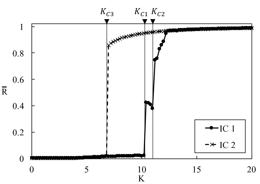
(a) $\Delta=1\,(q\approx 0.70)$

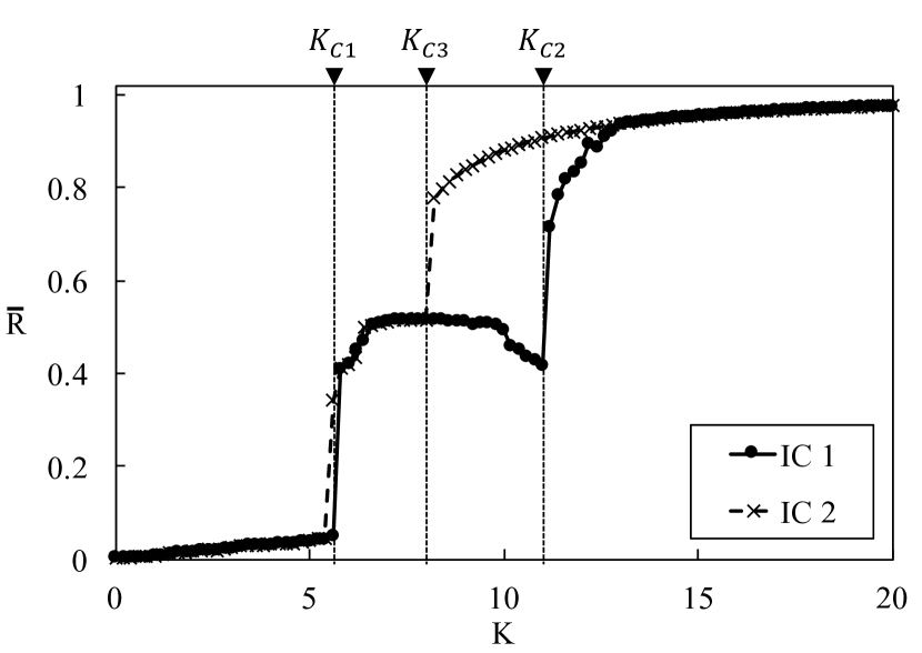
(b) $\Delta=1\,(q\approx 0.70)$

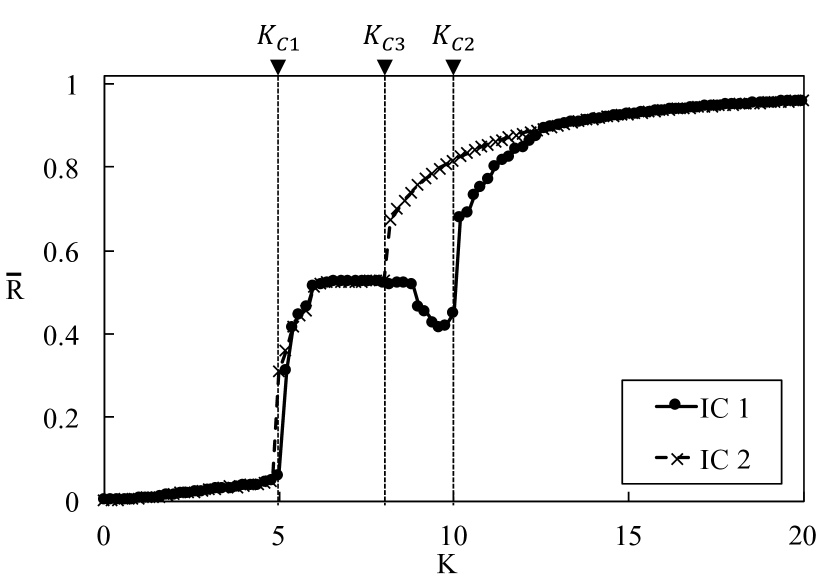
(c) $\Delta=0.6\,(q\approx 0.42)$

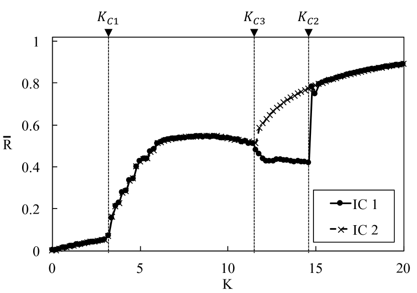
(d) $\Delta=0.6\,(q\approx 0.42)$

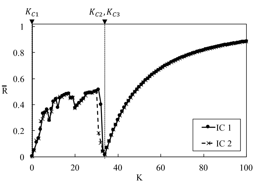
(e) $\Delta=0.2\,(q\approx 0.14)$

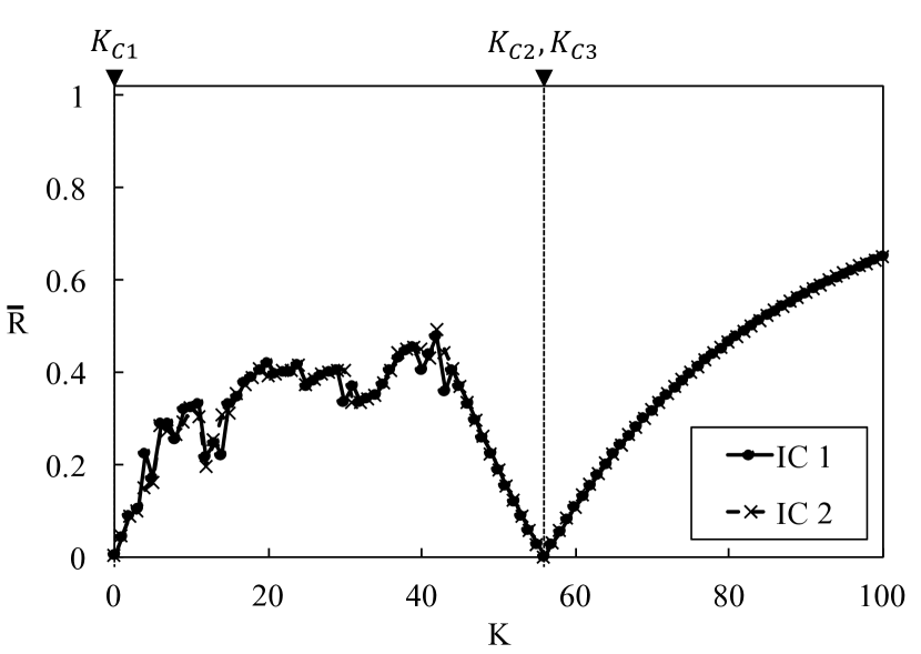
(f) $\Delta=0.2\,(q\approx 0.14)$

Figure 1. Comparison of the hysteretic loops of synchronization in case of different kernel radii. Results with zeroth and first order kernel-functions are shown on the left and right, respectively.

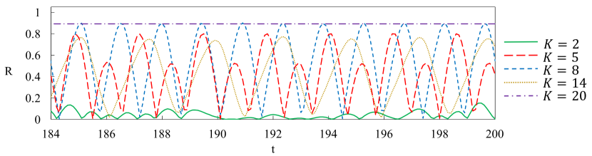
(a) •

(b) •

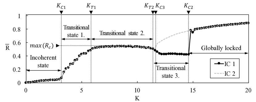
(c) •

Figure 2. States of a system of spatially coupled oscillators depending on the coupling parameter $K$. The relative kernel radius is $q\approx 0.46$, taking $\Delta=0.6$ and $\Delta x=0.05,N=400$ applying first order kernel-function. a) Time series of the order parameter $R$ for different values of $K$ calculated for IC 1. For $K_{C1}<K<K_{C2}$, $R$ has an oscillatory nature. b) Final phases of the oscillators in polar form at $t=500s$ illustrating the different states of the system calculated for IC 1. c) States of the system and the time average $\bar{R}$ of the order parameter depending on the coupling parameter $K$.

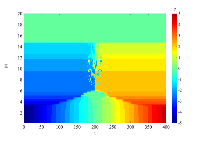
Figure 3.

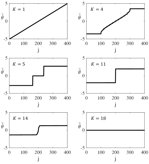
Figure 4.

4.2. States of the system

We analyzed the states of the spatially coupled model depending on the coupling parameter $K$ in case $q$ is large enough for the system to exhibit the hysteretic behavior. Analysis of the solutions of Eq. 7 in time was carried out by taking uniformly diffused initial conditions (IC 1) and first order kernel-function $W_{ij}^{1}$ with fixed kernel radius $\Delta=0.6$ ($q\approx 0.46$) and $\Delta x=0.05$. By examining the time evolution of the order parameter $R$ (Fig. 2A) and the phases of the individual oscillators (Fig. 2B), three states of the system in the $\bar{R}-K$ diagram (Fig. 2C) was found. 2B is only a visualization of the data and the distances measured on the circle are independent of the strength of the interactions. .

If $0<K<K_{C1}$, the system is in the incoherent state. Since we keep the natural frequency distribution defined by Eq. (8) and it is a dominant part of the equation, there are two in the initial configuration ($\Omega_{i}<0$ and $\Omega_{i}\geq 0$). The order parameter $R$ varies in time in a random-like manner, but it remains close to zero (Fig. 2A, $K=2$) and the phases of the oscillators are heterogeneous (Fig. 2B $K=2$). The fluctuations of $R$ in time can be attributed to the finite number of oscillators in the system. Increasing $K$, the average order parameter $\bar{R}$ stays near zero until reaching a $K_{C1}$ value. Above $K_{C1}$, the degree of synchronization gradually increases.

Increasing $K$ from $K_{C1}$, Note, that the overlap of the clusters neither result in their interaction nor global synchronization. Further increasing $K$, the system rapidly jumps into a globally locked state in a bifurcation point, at a $K_{C2}$ value. At this point, the clusters merge as one of them take over the domination

If $K_{C2}<K$, there is only one cluster, the system is in a globally locked state (Fig. 2B, $K=20$) and $R$ is constant in time (Fig. 2A, $K=20$). As $K$ is further increased, the synchronization and $\bar{R}$ gradually increases (Fig. 2A-B, $K=200$) and the system seemingly reaches the globally coherent state at a large value of $K$. In contrast to the fully coupled model, where $R\approx 1$ is reached at moderate $K$, here the results imply, that $\bar{R}\rightarrow 1$ asymptotically. Accordingly, spatial coupling can hinder full synchronization for large system sizes in case the coupling strength of the individual oscillators is limited.

We also checked the solutions of the model for IC 2. For $0\leq K\geq K_{C3}$, the system has the same states as for IC 1. Above $K_{C3}$, there is one globally locked cluster with constant $R$ in time.

Figure 5.

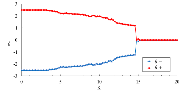
Figure 6.

4.3. Effect of the relative kernel radius

In Fig. 1, $\Delta$ and $q$ were varied simultaneously in the different simulations. The diagrams show varying values of $K_{C1},K_{C2},K_{C3}$ and different $max(R_{C})$ in the locally locked state. To examine the effect of the parameters separately, we calculated $\bar{R}$ versus $K$ for both IC 1 and IC 2 keeping either the number of oscillators in a neighborhood of a general point constant (i.e. keeping $\Delta$ and $\Delta x$ constant) or the relative kernel radius $q$ fixed. Since, there is no qualitative difference between the first and zeroth order kernel-functions, we applied $W_{ij}^{1}$ in all cases.

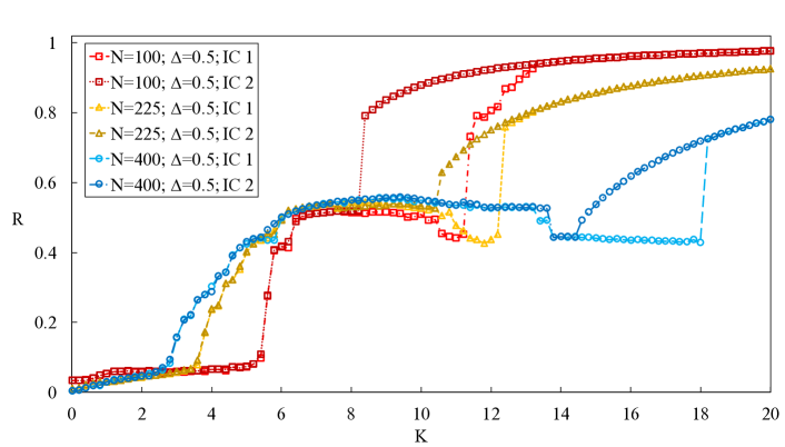
Figure 7. Average order parameter $\bar{R}$ versus the coupling parameter $K$ calculated for IC 1 and IC 2 fixing the kernel radius $\Delta=0.5$ and varying the domain size $L_{1}=0.5,L_{2}=0.75,L_{3}=1$ ($q_{1}\approx 0.7,q_{2}\approx 0.47,q_{3}\approx 0.35$), applying the first order kernel $W_{ij}^{1}$.

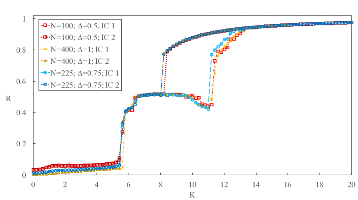
Figure 8.

As we can see in Fig. 7, although the number of oscillators in a general in-domain neighborhood is the same in all cases, both the local and global parts of the diagram are affected. In case of a smaller relative kernel radius, the local synchronization starts at smaller values of $K$ and a larger $K$ is necessary for the onset of the global synchronization. Furthermore, the maximal order $max(R_{C})$ of the system in the locally synchronized state is higher for $q_{2}$. Smaller relative kernel radius $q$ results in a larger range of $K$ corresponding to the locally synchronized states (i.e. $|K_{C1}-K_{C2}|$ increases), but it also requires a larger value of $K_{C3}$ for the global synchronization.

Fig. 8 shows, that there is only a small difference between the locations of $K_{C1}$ and $K_{C3}$, but the transitional state is not affected. The onset of the local synchronization requires larger $K$ as the system size is increased, but the global synchronization can be maintained for smaller values of $K$. Similar dependencies on the system size were reported in [10, 15] for the fully coupled and diluted systems, respectively. These results suggest, that the $\bar{R}-K$ diagram is characterized by $q$ and the local behavior is not affected by the system size. The maximal order $max({R_{C}})$ of the system in the locally synchronized state was also independent of the system size in our simulations.

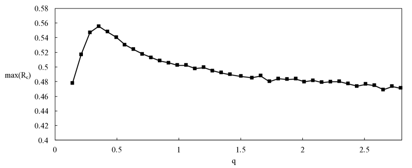
Figure 9. Maximum of the average order parameter in the locally locked state $max(R_{C})$ depending on $q$ fixing $L=1,\Delta x=0.05,N=400$, applying first order kernel-function. For the simplicity, the diagram was computed assuming IC 1.

Finally, we computed the maximal value of the order parameter in the locally locked state $\mathrm{max}(R_{C})$ for $K_{C1}<K<K_{C2}$ depending on $q$, keeping $L=1,\Delta x=0.05,N=400$ fixed and applying first order kernel-function. According to Fig. 9, the $max(R_{C})(q)$ function has a maximum. Consequently, there is an optimal value of the relative kernel radius in terms of the local synchronization. If $q$ is too large, the local behavior dominates and if the kernel radius is too small compared to the domain size, the local synchronization is hindered.

5. Conclusion

In summary, we carried out a numerical study to examine the effect of the spatial coupling of phase oscillators in the Kuramoto model with inertia. A finite size system was considered with compact zeroth and first order kernel functions to incorporate distance-dependent coupling strength between the oscillators. A dimensionless parameter, the relative kernel radius $q$ was introduced, expressing the ratio between the kernel radius and the maximal distance between the $i$th and $j$th oscillators. We examined the order of the global synchronization depending on the coupling parameter for different $q$ values. In the case of large kernel radii, the model gives back the original, fully coupled model.

We implemented the model in the Nauticle general purpose particle-based simulation tool [30] and examined the hysteretic behavior of the spatially coupled model. We fixed the domain size and investigated the behavior for different values of $q$. For a range of $q$, the system exhibits a hysteretic behavior depending on the initial conditions and the coupling parameter, but for a range of $K$ values locally locked clusters develop and dominate. In case of the presence of the local clusters, the order parameter $R$ is oscillates in time. We pointed out, that this oscillations can be attributed to locally locked clusters that develop and break up through some transitional states. If $q$ is small enough, the system exhibits no hysteresis, which agree with previous works showing that reducing the number of links between the oscillators lead to the vanish of the hysteretic behavior [15]. Analysis of the parameters in the problem showed, that the local behavior is characterized mainly by the relative kernel radius $q$, which has an optimal value leading to a maximal value of the synchronization in the locally locked state.

Our results suggest, that large systems of oscillators having a distance limited vision, such as the fireflies can develop locally synchronized clusters without transitioning into global synchronization. The proposed framework can be used to model more complex spatially coupled systems. Some bacteria such as Myxococcus xanthus [31] or systems of microgears [32] exhibit not only social interactions but also complex mechanical behavior. By the implementation of the model into Nauticle it is possible to consider a mathematical coupling of the Kuramoto model with other equations, such as mechanical models to examine complex systems of spatially moving oscillators.

References

- [1] Y. Kuramoto. International symposium on mathematical problems in mathematical physics. Lecture Notes in Theoretical Physics, 30:420, 1975. cited By 14.
- [2] Ziping Jiang and Martin McCall. Numerical simulation of a large number of coupled lasers. Journal of the Optical Society of America B, 10(1):155, jan 1993.
- [3] D. Cumin and C.P. Unsworth. Generalising the Kuramoto model for the study of neuronal synchronisation in the brain. Physica D: Nonlinear Phenomena, 226(2):181–196, feb 2007.
- [4] Ritwik K. Niyogi and L. Q. English. Learning-rate-dependent clustering and self-development in a network of coupled phase oscillators. Physical Review E, 80(6), dec 2009.
- [5] Yuri L. Maistrenko, Borys Lysyansky, Christian Hauptmann, Oleksandr Burylko, and Peter A. Tass. Multistability in the Kuramoto model with synaptic plasticity. Physical Review E, 75(6), jun 2007.
- [6] Di Yuan, Fang Lin, Limei Wang, Danyang Liu, Junzhong Yang, and Yi Xiao. Multistable states in a system of coupled phase oscillators with inertia. Scientific Reports, 7:42178, 2017.
- [7] T. J. Walker. Acoustic synchrony: two mechanisms in the snowy tree cricket. Science, 166(3907):891–894, nov 1969.
- [8] Bard Ermentrout. An adaptive model for synchrony in the firefly pteroptyx malaccae. Journal of Mathematical Biology, 29(6):571–585, 1991.
- [9] F.E. Hanson. Comparative studies of firefly pacemakers. In Federation proceedings, volume 37, pages 2158–2164, 1978.
- [10] Hisa Aki Tanaka, Allan J. Lichtenberg, and Shinichi Oishi. Self-synchronization of coupled oscillators with hysteretic responses. Physica D: Nonlinear Phenomena, 100(3-4):279–300, 1997.
- [11] B. R. Trees, V. Saranathan, and D. Stroud. Synchronization in disordered Josephson junction arrays: Small-world connections and the Kuramoto model. Physical Review E, 71(1), jan 2005.
- [12] F. Salam, J. Marsden, and P. Varaiya. Arnold diffusion in the swing equations of a power system. IEEE Transactions on Circuits and Systems, 31(8):673–688, aug 1984.
- [13] G. Filatrella, A. H. Nielsen, and N. F. Pedersen. Analysis of a power grid using a Kuramoto-like model. The European Physical Journal B, 61(4):485–491, feb 2008.
- [14] Martin Rohden, Andreas Sorge, Marc Timme, and Dirk Witthaut. Self-organized synchronization in decentralized power grids. Physical Review Letters, 109(6), aug 2012.
- [15] Simona Olmi, Adrian Navas, Stefano Boccaletti, and Alessandro Torcini. Hysteretic transitions in the Kuramoto model with inertia. Phys. Rev. E, 90:042905, Oct 2014.
- [16] Géza Ódor and Bálint Hartmann. Heterogeneity effects in power grid network models. Phys. Rev. E, 98:022305, Aug 2018.
- [17] N. Motee and Q. Sun. Sparsity measures for spatially decaying systems, June 2014.
- [18] Jan Sieber and Tamás Kalmár-Nagy. Stability of a chain of phase oscillators. Physical Review E, 84(1):016227, 2011.
- [19] G. H Paissan and D. H Zanette. Synchronization and clustering of phase oscillators with heterogeneous coupling. Europhysics Letters (EPL), 77(2):20001, jan 2007.
- [20] Liudmila Tumash, Simona Olmi, and Eckehard Schöll. Effect of disorder and noise in shaping the dynamics of power grids. EPL (Europhysics Letters), 123(2):20001, 2018.
- [21] Thomas K DM Peron, Peng Ji, Francisco A Rodrigues, and Jürgen Kurths. Effects of assortative mixing in the second-order Kuramoto model. Physical Review E, 91(5):052805, 2015.
- [22] Can Xu, Yuting Sun, Jian Gao, Tian Qiu, Zhigang Zheng, and Shuguang Guan. Synchronization of phase oscillators with frequency-weighted coupling. Scientific Reports, 6:21926, 2016.
- [23] Hui Wu, Ling Kang, Zonghua Liu, and Mukesh Dhamala. Exact explosive synchronization transitions in Kuramoto oscillators with time-delayed coupling. Scientific Reports, 8(1), oct 2018.
- [24] B. Ermentrout and J. Rinzel. Beyond a pacemaker’s entrainment limit: phase walk-through. American Journal of Physiology-Regulatory, Integrative and Comparative Physiology, 246(1):R102–R106, 1984.
- [25] Michael Breakspear, Stewart Heitmann, and Andreas Daffertshofer. Generative models of cortical oscillations: neurobiological implications of the Kuramoto model. Frontiers in human neuroscience, 4:190, 2010.
- [26] Angelo Cenedese and Chiara Favaretto. On the synchronization of spatially coupled oscillators. 2015.
- [27] Tomasz Kapitaniak, Patrycja Kuzma, Jerzy Wojewoda, Krzysztof Czolczynski, and Yuri Maistrenko. Imperfect chimera states for coupled pendula. Scientific reports, 4:6379, 2014.
- [28] Xiang Li and Pengchun Rao. Synchronizing a weighted and weakly-connected Kuramoto-oscillator digraph with a pacemaker. IEEE Transactions on Circuits and Systems I: Regular Papers, 62(3):899–905, mar 2015.
- [29] Donald Shepard. A two-dimensional interpolation function for irregularly-spaced data. In Proceedings of the 1968 23rd ACM national conference, pages 517–524. ACM, 1968.
- [30] Balázs Tóth. Nauticle: a general-purpose particle-based simulation tool. CoRR, abs/1710.08259, 2017.
- [31] Simone Leonardy, Gerald Freymark, Sabrina Hebener, Eva Ellehauge, and Lotte Søgaard-Andersen. Coupling of protein localization and cell movements by a dynamically localized response regulator in myxococcus xanthus. The EMBO Journal, 26(21):4433–4444, 2007.
- [32] Antoine Aubret, Mena Youssef, Stefano Sacanna, and Jérémie Palacci. Targeted assembly and synchronization of self-spinning microgears. Nature Physics, 14(11):1114–1118, jul 2018.