Polarisation as a tracer of CMB anomalies:
Planck results and future forecasts
Abstract
The lack of power anomaly is an intriguing feature at the largest angular scales of the CMB anisotropy temperature pattern, whose statistical significance is not strong enough to claim any new physics beyond the standard cosmological model. We revisit the former statement by also considering polarisation data. We propose a new one-dimensional estimator which takes jointly into account the information contained in the TT, TE and EE CMB spectra. By employing this estimator on Planck 2015 low- data, we find that a random CDM realisation is statistically accepted at the level of . Even though Planck polarisation contributes a mere to the total information budget, its use pushes the lower-tail-probability down from the obtained with only temperature data. Forecasts of future CMB polarised measurements, as e.g. the LiteBIRD satellite, can increase the polarisation contribution up to times with respect to Planck at low-. We argue that the large-scale E-mode polarisation may play an important role in analysing CMB temperature anomalies with future mission.
keywords:
Lack of Power , CMB anomalies , CMB polarisation , CMB1 Introduction
CMB observations show anomalies at large angular scale of the temperature map, see e.g. [1]. The statistical level of these signatures is around 2-3 from what expected in the concordance CDM model. Not all of these anomalies are independent and a certain degree of correlation exists [2]. Here we focus on the lack of power anomaly: the temperature CMB anisotropy pattern exhibits less power with respect to what foreseen by CDM. This effect has been studied with the variance estimator in WMAP data [3, 4, 5] and in Planck 2013 [6] and Planck 2015 [7] data, measuring a lower-tail-probability of the order of few per cent. Such a percentage can become even smaller, below , once only regions at high Galactic latitude are taken into account [5].
WMAP and Planck agree well on this feature, so it is very hard, albeit not impossible, to attribute this anomaly to systematic effects of instrumental origin. Moreover it is also difficult to believe that a lack of power could be generated by residuals of astrophysical emission, since the latter is not expected to be correlated111In particular they should be anti-correlated to produce a decrease of the total power. with the CMB and therefore an astrophysical residual should increase the total power rather than decreasing it. Hence, it appears natural to accept this as a real feature present in the CMB pattern.
An early fast-roll phase of the inflaton could naturally explain such a lack of power, see e.g. [8, 9, 10, 11, 12]: this anomaly might then witness a new cosmological phase before the standard inflationary era (see e.g. [13, 14, 15]).
However, with only the observations based on the temperature map, this anomaly is not statistically significant enough to be used to claim new physics beyond the standard cosmological model. Therefore, it is legitimate to conservatively interpret it as a statistical fluke of the CDM concordance model.
The main point of this paper is to argue that future CMB polarisation data at low- might increase the significance of this anomaly. In other words, considering the counterpart in polarisation of the lack of power currently observed in temperature might be key to confirm it as a simple statistical fluke or to raise it up at the level of manifestation of new physics222Of course this argument might be used for any CMB anomaly..
In this paper we propose a new one-dimensional estimator which combines information from the CMB TT, EE and TE angular power spectra at the largest angular scales, i.e. , with being the multipole moment. Considering Planck data in the whole harmonic range mentioned above, noise dominated polarisation provides an information content at the level of to this estimator which, even though small, has a non-negligible impact on the analysis, the lower-tail-probability shifting downward from (obtained considering only temperature data) to C.L. (obtained considering jointly temperature and polarisation data). We show that for future CMB observations, polarisation at the largest angular scales can weight as much as of the total information entering our estimator.
We argue that the inclusion of large-scale E-mode polarisation could crucially help in changing the interpretation from a simple statistical fluke into the detection of a new physical phenomenon. Therefore, future CMB large-scale polarised observations, which are typically aimed at primordial B-modes, might provide signals of new physics also through the other polarised CMB mode, i.e. the E-mode.
The paper is organised as follows: in Section 2 we introduce the algebra needed to build the new estimator which condensates all the TT, EE and TE information into a 1-D object; in Section 3 we elaborate on an optimised (i.e. minimum variance) version of the proposed estimator; Section 4 is devoted to the description of the dataset used and of the simulations employed; in Section 5 we present the results on Planck data and provide estimates of the improvement expected with future CMB polarised observations, as the LiteBIRD satellite [16]; conclusions are drawn in Section 6.
2 A new one-dimensional joint estimator: the dimensionless normalised mean power
The idea of this joint estimator starts from the usual equations employed to simulate temperature and E-mode CMB maps, see e.g. [17]:
| (1) | |||||
| (2) |
where are the coefficients of the Spherical Harmonics (with being integers numbers so that and ), , and are the theoretical angular power spectra (APS) for , and and with being Gaussian random variables, uncorrelated, with zero mean and unit variance:
| (3) | |||||
| (4) | |||||
| (5) | |||||
| (6) |
From equations (1),(2) one can compute the corresponding APS, defined as
| (7) | |||||
| (8) | |||||
| (9) |
where the label stands for “simulated”, i.e. realised randomly from the theoretical spectra , and , finding the following expressions,
| (10) | |||||
| (11) | |||||
| (12) |
where are vectors with components, i.e.
| (13) |
and is defined as
| (14) |
It is easy to check that taking the ensemble average of equations (10),(11) and (12) yields to
| (15) | |||||
| (16) | |||||
| (17) |
since for each , as a consequence of equations (5),(6),
| (18) | |||||
| (19) | |||||
| (20) |
Equations (10),(11) and (12) can be inverted, giving the following set of equations
| (21) | |||||
| (22) | |||||
| (23) |
where we have dropped out the label “” for sake of simplicity. Now, we can interpret , and as the CMB APS recovered by a CMB experiment under realistic circumstances, i.e. including noise residuals, incomplete sky fraction and finite angular resolution333In principle one can also include residuals of systematic effects.. Once the model is chosen, i.e. once the spectra , and are fixed, for example to CDM, one can compute the following objects
| (24) | |||||
| (25) | |||||
| (26) |
for the observations and/or for the corresponding realistic simulations.
In the following we will call the variables , and as APS of the normal random variables or normalised APS (henceforth NAPS). The advantage of using NAPS, instead of the standard APS, is that they are dimensionless and similar amplitude numbers and can be easily combined to define a 1-D estimator in harmonic space, which depends on temperature, E-mode polarisation and their cross-correlation. A natural definition of this 1-D estimator, called , is the following
| (27) |
The estimator could be interpreted as a dimensionless normalised mean power, which jointly combines the temperature and polarisation data. The expectation value of is
| (28) |
regardless of the value of . Note that a definition of the following type
| (29) |
is expected to have less signal-to-noise ratio with respect to because while and have the same expectation value, the intrinsic variance of is in general smaller than the one of .
We will see in the following that Eq. (27) is noise-limited for Planck data due to (its polarisation part) and in practice can be employed only up to . An optimised version of this estimator, given in Section 3, does not suffer from this issue and can be employed up to the maximum multipole considered in this analysis, i.e. .
3 Optimised estimator
In equation (27) the NAPS and are combined with equal weights. However the signal-to-noise ratios of the two NAPS are different even in the cosmic variance limit case: therefore one might wonder which are the best weights that we can use in the definition of the joint estimator in order to make it optimal, i.e. with minimum variance. It is possible to show, see A, that the optimised estimator , defined as
| (30) |
has minimum variance when
| (31) | |||
| (32) |
where and stand respectively for the variance and the covariance of the variables which appear in the brackets. These coefficients, namely and as defined in Eqs.(31-32), will be actually used to build the estimator. Note that as done for , , which depends on , has been normalised such that for any value of . Note also, that can be employed up to both for Planck and LiteBIRD-like simulated data: what changes between the two cases is the set of the coefficients and , or, in other words, the relative contribution of the temperature and polarisation data.
4 Dataset and simulations
We use the latest public Planck satellite CMB temperature data444http://www.cosmos.esa.int/web/planck/pla. i.e. the Planck 2015 Commander map with its standard mask () entering the temperature sector of the low- Planck likelihood555At the moment of writing the corresponding Planck 2018 likelihood code and corresponding data set is not publicly available. [18]. In polarisation we consider a noise-weighted combination of WMAP9 and Planck data as done in [19]. This allows to gain some signal-to-noise ratio and to deal with a larger sky fraction in polarisation (). Temperature and polarisation maps are sampled at HEALPix666http://healpix.sourceforge.net/. [20] resolution . For sake of simplicity we will refer to this data set as the Planck-WMAP low- data set.
In order to build the estimators and , as defined in equations (27) and (30), we estimate the six CMB APS from simulated CMB-plus-noise maps. The signal is extracted from the Planck fiducial CDM model defined by the following parameters
being the baryon density, the cold dark matter density, the angle subtended by the sound horizon at recombination, the re-ionization optical depth, the amplitude and the spectral index of primordial scalar perturbations. This set of parameters is obtained confronting data and models through the likelihood function defined as the sum of the three following likelihoods (see [18, 19] for further details):
-
1.
a pixel based low- likelihood, , where the Planck 2015 Commander map enters the temperature sector and a noise-weighted combination of WMAP9 and Planck data enters the polarisation sector of this likelihood777Note that the low- data-set used to perform the analysis is exactly the same as the one entering the low- likelihood. This makes the whole investigation self-consistent.;
-
2.
a high- Planck TT likelihood based on APS of Planck data in the range ;
-
3.
the Planck lensing likelihood, based on the range of the four-point correlation function of the temperature anisotropies.
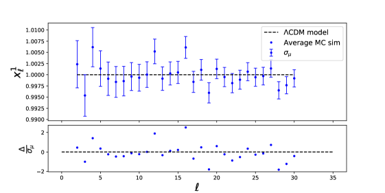
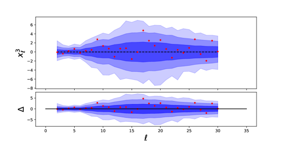
The noise of the simulated maps is generated through Cholesky decomposition of the total noise covariance matrix in pixel space, see B. Such estimates are obtained over the observed sky fraction, with the optimal angular power spectrum estimator BolPol [22]. Montecarlo simulations for the Planck-WMAP low- data set are validated in Figure 1, where the average of the NAPS (, and ) are shown respectively in the upper, middle and lower panels along with their uncertainties of the means (). Each panel displays also a lower box where for each it is shown the distance of mean in units of standard deviation of the mean itself.
 |
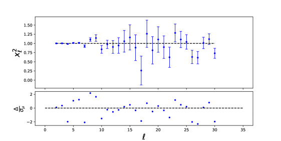 |
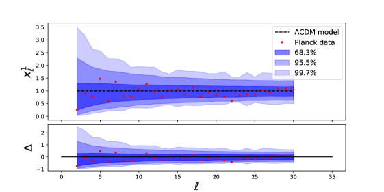
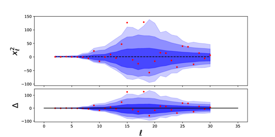
Figure 2 shows the low- estimates of , and of the Planck-WMAP low- data set (red dots), with the contours at one, two and three as estimated from simulations (blue regions).
 |
 |
 |
Simulations for a LiteBIRD-like noise level [21] are obtained following the same procedure as described above but dividing the polarisation part of the noise covariance matrix by a factor of .
The choice of the parameter, which enters the definition of , see eq.(27), is dictated by the signal-to-noise ratio of since is always signal dominated in the whole range considered. In Figure 3 we display the signal-to-noise ratio (), see C, of the NAPS for the Planck-WMAP low- data set (see solid lines). While for such a ratio grows monotonically (red line), for (solid blue line) it saturates around . Consequently we will employ the estimator with for the Planck-WMAP low- data set.
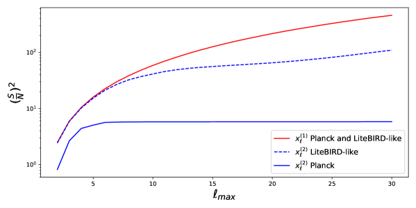 |
The signal-to-noise ratio of for the LiteBIRD-like noise level is instead shown in Figure 3 as a dashed blue line. Since such a ratio grows monotonically, in this case we can choose the maximum available in our simulations, i.e. .
5 Results of the analyses
5.1 Results for
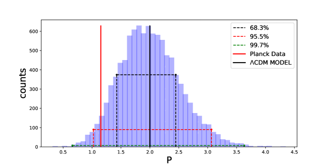
In Figure 4 we plot the empirical distribution expected in CDM for with considering the Planck-WMAP low- characteristics. The red vertical line stands for the observed value of the Planck-WMAP low- data set. The lower-tail probability (LTP) of the observed value of is . Such a value is smaller than the corresponding LTP of when, still with , we neglect the contribution of in eq. (27). In that case the LTP we obtain is . Similarly for the same maximum multipole, when we neglect the contribution of in , we get a LTP of . In short, the combination of temperature and polarisation data provides a LTP smaller than what obtained with only temperature or only polarisation, although our findings cannot be considered as statistically anomalous.
 |
In Figure 5 we plot the empirical distribution of expected in CDM with for the Planck-WMAP low- data set and for the LiteBIRD-like noise level.
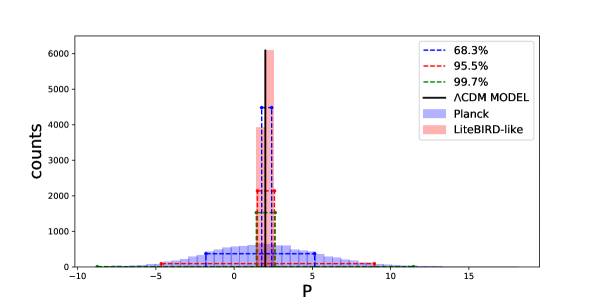 |
In order to evaluate the improvement of the latter with respect to the former, we build the ratios between the widths of the empirical distributions of , corresponding to the level of , for the LiteBIRD-like noise level () and for the Planck-WMAP low- noise level (). We find that the width of the estimator in the LiteBIRD case can be even times smaller with respect to what obtained in the Planck-WMAP low- case, if .
5.2 Results for
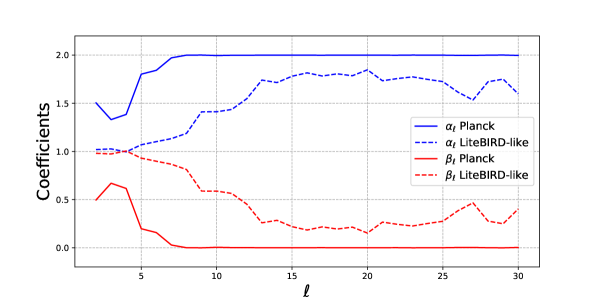
In Figure 6 we plot and (see equations (31) and (32)) as a function of for the Planck-WMAP low- data set (solid lines). Note how for go to zero (and consequently for same multipoles) because of the noise level in polarisation.
 |
For , even though the distribution of is narrower with respect to shown in Figure 4, Planck-WMAP low- data shift a little so that the LTP is increased to . However , as already mentioned, is not limited in the choice of and still for the Planck-WMAP low- data at we obtain a LTP at the level of . In Figure 7 we give the LTP for at each , displayed in black, compared to a naive estimator defined only with temperature data as
shown in blue.
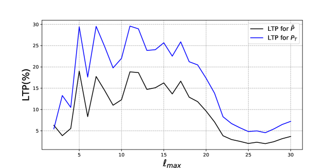 |
It is interesting to note how the inclusion of the subdominant polarisation part impacts on the analysis making the LTP of smaller then for the whole range considered. In particular for at we compute that the LTP is .
Still in Figure 6 we plot and as a function of for the LiteBIRD-like noise level (see dashed lines). Note that for this case none of the go to zero and therefore polarisation data provide a contribution for each of the multipoles considered at large scale. Correspondently temperature data will not saturate the information entering for any considered multipoles.
In order to evaluate the impact of polarisation and temperature data on we define the following weights
| (33) | |||
| (34) |
such that for every .
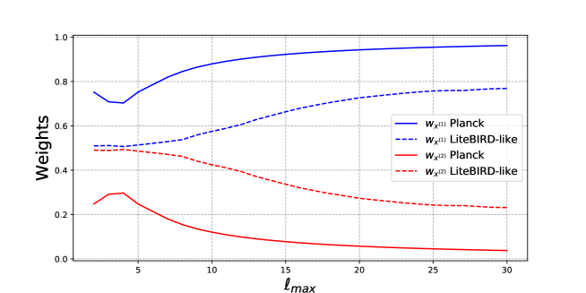 |
For we find that polarised Planck-WMAP low- data contribute at the level of to the building of . This value increases to for future LiteBIRD-like polarised data at the same maximum multipole. At we forecast that future LiteBIRD-like polarised data will weight as the with respect to the obtained with Planck-WMAP low- data, therefore providing an increasing factor . The behaviour of and for each is given in Figure 8.
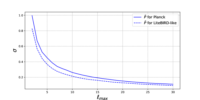
We end this Section showing in Figure 9 how the standard deviation of shrinks for each from current Planck data (solid blue) to future LiteBIRD-like data (dashed blue). We compute that at low- future data will allow to build with a statistical uncertainty that will be around smaller with respect to current Planck data.
 |
6 Conclusions
In this paper we have proposed a new one-dimensional estimator, i.e. and its optimised version , see equations (27) and (30), which is able to jointly test the lack of power in TT, TE and EE. The main outcomes of this analysis are listed below.
-
1.
Considering Planck-WMAP low- data it is interesting to note that the inclusion of polarisation information through our new one-dimensional estimator, either or , provides estimates which are less likely accepted in a CDM model than the corresponding only-temperature version of the same estimator. In other words, polarisation though subdominant in terms of signal-to-noise ratio with respect to temperature, plays a non-negligible role in the evaluation of compatibility between data and the standard model. However the LTP obtained are at the level of few per cent and therefore still compatible with a statistical fluke. See for instance Figure 7: even though the weight of polarisation data is only around of the total information budget, the LTP probability of is always smaller than its corresponding temperature-only version .
-
2.
E-modes at large angular scale still contain information which might be capable to probe new physics beyond the standard cosmological model.
-
(a)
We forecast that future CMB polarised measurements à la LiteBIRD can tight the empirical distribution of up to a factor of .
-
(b)
Considering the optimised version of the proposed estimator, i.e. , we evaluate that future LiteBIRD-like measurements can shrink the statistical uncertainty by and at the same time increasing the contribution of the polarisation part by a factor ranging from to .
-
(a)
Future all-sky CMB experiments aimed at detecting primordial B-modes (which in turn are related to the energy scale of inflation) are designed to observe CMB polarisation with exquisite accuracy and precision. In order to make this possible, residual systematic effects both of instrumental and astrophysical origin have to be carefully measured or, at least, kept under control. In this paper we suppose that this is the case and that the statistical noise is the dominant source of uncertainty. Under these circumstances, E-modes will be in practice known at the cosmic variance limit at large angular scales. This is a great opportunity, since E-mode polarisation might contain important information about the lack of power anomaly currently observed only in the temperature map, which could be tracing new physical phenomena beyond the standard cosmological model in the early universe.
Appendix A Computation of the weights for
We use the method of the Lagrange multipliers to minimise the variance of , i.e. , keeping fixed the expected value of . This can be achieved requiring that
| (35) |
for each multipole . Replacing the definition of , see equation (30), in the expression of , one obtains
| (36) | |||||
where the cross-terms among different multipoles goes exactly to zero in the full sky case, and with defined as
| (37) |
where the barred quantities are defined as and where and are the variance of and respectively, and is their covariance
| (38) |
Because of Eq. (36), the minimisation of is equivalent to the minimisation of each . As it is customary in the Lagrange multiplier method, for each multipole we introduce a new variable , known as the Lagrange multiplier, and minimise the function which is defined as
| (39) |
This is equivalent to minimise the variance of on the constrain given by equation (35) (multiplied by ). Therefore we compute the partial derivatives with respect to the coefficients , and and set them to be zero:
| (40) | |||||
| (41) | |||||
| (42) |
This set of equations is solved by equations (31), (32) together with
| (43) |
Appendix B Noise generation through Cholesky decomposition
Given a noise covariance matrix defined over the observed pixels, it is possible to generate a noise map, , statistically compatible with , through the following expression
| (44) |
where is the lower triangular matrix of the Cholesky decomposition [23] such that
| (45) |
and is a vector with the same dimension as and whose entries are randomly extracted from a normal distribution. In this way turns out to be statistically compatible with since
| (46) |
where is the identity matrix and stands for ensamble average.
Appendix C Signal-to-noise ratio
The total signal-to-noise ratio contained in or up to a maximum harmonic scale , is defined summing up over the multipoles from to as:
| (47) |
where
| (48) |
since , for .
Acknowledgments
We acknowledge the use of computing facilities at NERSC (USA), of the HEALPix package [20], and of the Planck Legacy Archive (PLA). This research was supported by ASI through the Grant 2016-24-H.0 (COSMOS) and through the ASI/INAF Agreement I/072/09/0 for the Planck LFI Activity of Phase E2, and by INFN (I.S. FlaG, InDark). L.M. acknowledges the PRIN MIUR 2015 “Cosmology and fundamental physics: illuminating the dark universe with Euclid”.
References
References
- [1] D. J. Schwarz, C. J. Copi, D. Huterer and G. D. Starkman, Class. Quant. Grav. 33 (2016) no.18, 184001 [arXiv:1510.07929 [astro-ph.CO]].
- [2] J. Muir, S. Adhikari and D. Huterer, arXiv:1806.02354 [astro-ph.CO].
- [3] C. Monteserin, R. B. B. Barreiro, P. Vielva, E. Martinez-Gonzalez, M. P. Hobson and A. N. Lasenby, Mon. Not. Roy. Astron. Soc. 387 (2008) 209 [arXiv:0706.4289 [astro-ph]].
- [4] M. Cruz, P. Vielva, E. Martinez-Gonzalez and R. B. Barreiro, Mon. Not. Roy. Astron. Soc. 412 (2011) 2383 [arXiv:1005.1264 [astro-ph.CO]].
- [5] A. Gruppuso, P. Natoli, F. Paci, F. Finelli, D. Molinari, A. De Rosa and N. Mandolesi, JCAP 1307 (2013) 047 [arXiv:1304.5493 [astro-ph.CO]].
- [6] P. A. R. Ade et al. [Planck Collaboration], Astron. Astrophys. 571 (2014) A23 doi:10.1051/0004-6361/201321534 [arXiv:1303.5083 [astro-ph.CO]].
- [7] P. A. R. Ade et al. [Planck Collaboration], Astron. Astrophys. 594 (2016) A16 [arXiv:1506.07135 [astro-ph.CO]].
- [8] C. R. Contaldi, M. Peloso, L. Kofman and A. D. Linde, JCAP 0307 (2003) 002 doi:10.1088/1475-7516/2003/07/002 [astro-ph/0303636].
- [9] J. M. Cline, P. Crotty and J. Lesgourgues, JCAP 0309 (2003) 010 doi:10.1088/1475-7516/2003/09/010 [astro-ph/0304558].
- [10] C. Destri, H. J. de Vega and N. G. Sanchez, Phys. Rev. D 81 (2010) 063520 doi:10.1103/PhysRevD.81.063520 [arXiv:0912.2994 [astro-ph.CO]].
- [11] M. Cicoli, S. Downes and B. Dutta, JCAP 1312 (2013) 007 doi:10.1088/1475-7516/2013/12/007 [arXiv:1309.3412 [hep-th]].
- [12] E. Dudas, N. Kitazawa, S. P. Patil and A. Sagnotti, JCAP 1205 (2012) 012 [arXiv:1202.6630 [hep-th]]; N. Kitazawa and A. Sagnotti, JCAP 1404 (2014) 017 [arXiv:1402.1418 [hep-th]], EPJ Web Conf. 95 (2015) 03031 [arXiv:1411.6396 [hep-th]], Mod. Phys. Lett. A 30 (2015) no.28, 1550137 [arXiv:1503.04483 [hep-th]].
- [13] A. Gruppuso and A. Sagnotti, Int. J. Mod. Phys. D 24 (2015) no.12, 1544008 [arXiv:1506.08093 [astro-ph.CO]].
- [14] A. Gruppuso, N. Kitazawa, N. Mandolesi, P. Natoli and A. Sagnotti, Phys. Dark Univ. 11 (2016) 68 [arXiv:1508.00411 [astro-ph.CO]].
- [15] A. Gruppuso, N. Kitazawa, M. Lattanzi, N. Mandolesi, P. Natoli and A. Sagnotti, Phys. Dark Univ. 20 (2018) 49 doi:10.1016/j.dark.2018.03.002 [arXiv:1712.03288 [astro-ph.CO]].
- [16] A. Suzuki et al., arXiv:1801.06987 [astro-ph.IM].
- [17] C. J. Copi, D. Huterer, D. J. Schwarz and G. D. Starkman, Mon. Not. Roy. Astron. Soc. 434 (2013) 3590 doi:10.1093/mnras/stt1287 [arXiv:1303.4786 [astro-ph.CO]].
- [18] N. Aghanim et al. [Planck Collaboration], Astron. Astrophys. 594 (2016) A11 doi:10.1051/0004-6361/201526926 [arXiv:1507.02704 [astro-ph.CO]].
- [19] M. Lattanzi et al., JCAP 1702 (2017) no.02, 041 doi:10.1088/1475-7516/2017/02/041, 10.1088/1475- [arXiv:1611.01123 [astro-ph.CO]].
- [20] K. M. Gorski, E. Hivon, A. J. Banday, B. D. Wandelt, F. K. Hansen, M. Reinecke and M. Bartelman, Astrophys. J. 622 (2005) 759 doi:10.1086/427976 [astro-ph/0409513]. http://sourceforge.net/projects/healpix/.
- [21] T. Matsumura et al., J. Low. Temp. Phys. 176 (2014) 733 doi:10.1007/s10909-013-0996-1 [arXiv:1311.2847 [astro-ph.IM]].
- [22] A. Gruppuso, A. De Rosa, P. Cabella, F. Paci, F. Finelli, P. Natoli, G. de Gasperis and N. Mandolesi, Mon. Not. Roy. Astron. Soc. 400 (2009) 463 doi:10.1111/j.1365-2966.2009.15469.x [arXiv:0904.0789 [astro-ph.CO]].
- [23] W. H. Press, S. A. Teukolsky, W. T. Vetterling, B. P. Flannery “Numerical Recipes 3rd Edition: The Art of Scientific Computing”, 2007 isbn: 0521880688, 9780521880688, Cambridge University Press, New York, NY, USA.