The white dwarf mass–radius relation and its dependence on the hydrogen envelope.

Abstract

We present a study of the dependence of the mass–radius relation for DA white dwarf stars on the hydrogen envelope mass and the impact on the value of $\log g$, and thus the determination of the stellar mass. We employ a set of full evolutionary carbon-oxygen core white dwarf sequences with white dwarf mass between 0.493 and $1.05M_{\odot}$. Computations of the pre-white dwarf evolution uncovers an intrinsic dependence of the maximum mass of the hydrogen envelope with stellar mass, i.e., it decreases when the total mass increases. We find that a reduction of the hydrogen envelope mass can lead to a reduction in the radius of the model of up to $\sim 12\%$. This translates directly into an increase in $\log g$ for a fixed stellar mass, that can reach up to 0.11 dex, mainly overestimating the determinations of stellar mass from atmospheric parameters. Finally, we find a good agreement between the results from the theoretical mass–radius relation and observations from white dwarfs in binary systems. In particular, we find a thin hydrogen mass of $M_{H}\sim 2\times 10^{-8}M_{\odot}$, for 40 Eridani B, in agreement with previous determinations. For Sirius B, the spectroscopic mass is 4.3% lower than the dynamical mass. However, the values of mass and radius from gravitational redshift observations are compatible with the theoretical mass–radius relation for a thick hydrogen envelope of $M_{H}=2\times 10^{-6}M_{\odot}$.

1 Introduction

One of the results of Chandrasekhar’s theory for the structure of white dwarf stars is a dependence of the radius with the stellar mass, known as the mass–radius relation. This relation is widely used in stellar astrophysics. It makes possible to estimate the stellar mass of white dwarf stars from spectroscopic temperatures and gravities, which in turn are used to determine the mass distribution (see e.g., Koester et al., 1979; Bergeron et al., 2001; Liebert et al., 2005; Holberg et al., 2012; Falcon et al., 2012; Tremblay et al., 2017). In addition, a determination of the white dwarf mass distribution contains information about the star formation history and is directly related with the initial–final mass function (Catalán et al., 2008; Cummings et al., 2016; El-Badry et al., 2018) which determines how much stellar material is returned to the interstellar medium, affecting the chemical evolution of the Galaxy.

Semi-empirical determinations of the mass–radius relations can be obtained from atmospheric parameters, effective temperature and surface gravity, which combined with flux measurements and parallax, can lead to a determination of the radius and stellar mass (Provencal et al., 1998; Holberg et al., 2012; Bédard et al., 2017). This technique started with the works by Schmidt (1996) and Vauclair et al. (1997), who used atmospheric parameters and trigonometric parallax measurements for 20 white dwarfs observed with the Hypparcos satellite. Later, this technique was expanded to include wide binary systems for which the primary has a precise parallax from Hipparcos (Provencal et al., 1998; Holberg et al., 2012) and Gaia DR1 (Tremblay et al., 2017). However, this method is not completely independent of theoretical models, since the determination of the radius depends on the flux emitted at the surface of the star, that is based on the predictions of model atmospheres. In addition, the determinations of the effective temperature and surface gravity also rely on model atmospheres, usually through spectral fitting, which can suffer from large uncertainties, up to $\sim 0.1$ in $\log g$ and 1–10% in temperature (Joyce et al., 2018a; Tremblay et al., 2019).

For eclipsing binary systems, the mass and radius of the white dwarf component can be obtained from photometric observations of the eclipses and kinematic parameters, without relying on white dwarf model atmospheres, except for the determination of the effective temperature. However, the specific configuration of eclipsing binaries implies that they have most probably interacted in the past, as common-envelope binaries (Tremblay et al., 2017). A sample of eclipsing binaries containing a white dwarf component applied to the study of the mass–radius relation can be found in Parsons et al. (2010, 2012a, 2012b, 2017). In particular, Parsons et al. (2017) analysed a sample of 16 white dwarfs in detached eclipsing binary and estimated their mass and radius up to a precision of 1–2 per cent.

Another method to test the mass–radius relation is to rely on astrometric binaries with precise orbital parameters, in particular a dynamical mass determination, and distances. Examples of those systems are Sirius, 40 Eridani and Procyon, for which recent determinations of the dynamical masses based on detailed orbital parameters were reported by Bond et al. (2017a), Mason et al. (2017) and Bond et al. (2015), respectively. However, the radius of the white dwarf component cannot be determined from orbital parameters and other techniques are necessary to estimate this parameters. In particular, for the systems mentioned above, the radius is estimated from the measured flux and precise parallax, depending on model atmospheres.

From evolutionary model computations for single stars it is known that the theoretical mass–radius relation depends systematically on effective temperature, core composition, helium abundance and hydrogen abundance in the case of DA white dwarf stars (Wood, 1995; Fontaine et al., 2001; Renedo et al., 2010; Salaris et al., 2010; Romero et al., 2015). Previous theoretical mass–radius relations (e.g. Wood, 1995; Fontaine et al., 2001) have assumed a constant hydrogen layer thickness which is applied to all models regardless of progenitor and white dwarf mass, being typically $M_{H}/M_{*}=10^{-4}$ (Iben & Tutukov, 1984). However, full evolutionary computations from Romero et al. (2012, 2013) showed that the upper limit for the mass of the hydrogen layer in DA white dwarf depends on the total mass of the remnant. The hydrogen content can vary from $M_{H}/M_{*}\sim 10^{-3}$, for white dwarf masses of $\sim 0.5M_{\odot}$, to $M_{H}/M_{*}=10^{-6}$ for massive white dwarfs with $\sim 1M_{\odot}$. In addition, asteroseismological studies show strong evidence of the existence of a hydrogen layer mass range in DA white dwarfs, within the range $10^{-9.5}<M_{H}/M_{*}<10^{-4}$, with an average of $M_{H}/M_{*}\sim 10^{-6.3}$ (Fontaine & Brassard, 2008; Castanheira & Kepler, 2009; Romero et al., 2012). The mass of the hydrogen layer is an important factor, since the mass–radius relation varies by 1-15 per cent, depending on the white dwarf mass and temperature, whether a thick ($10^{-4}M_{*}$) or a thin ($10^{-10}M_{*}$) hydrogen layer is assumed (Tremblay et al., 2017).

In this work we study the dependence of the mass–radius relation with the mass of the hydrogen layer. The white dwarf cooling sequences employed are those from Romero et al. (2012, 2013, 2017), extracted from the full evolutionary computations using the LPCODE evolutionary code (Althaus et al., 2005; Renedo et al., 2010). The model grid expands from $\sim 0.493M_{\odot}$ to $1.05M_{\odot}$ in white dwarf mass, where carbon-oxygen core white dwarfs are found. We also consider a range in hydrogen envelope mass from $\sim 10^{-3}M_{*}$ to $\sim 5\times 10^{-10}M_{*}$, depending on the stellar mass.

We compare our theoretical sequences with mass and radius determinations for white dwarfs in binary systems, in order to test the predictions of the theoretical mass–radius relation and to measure the hydrogen content in the star, when possible. We consider four white dwarfs in astromeric binaries – 40 Eridani B (Mason et al., 2017), Sirius B (Bond et al., 2017a), Procyon B (Bond et al., 2015) and Stein 2051 B (Sahu et al., 2017) – and a sample of 11 white dwarfs in detached eclipsing binaries (Parsons et al., 2017).

The paper is organized as follows. In section 2 we briefly describe the evolutionary cooling sequences used in our analysis. Section 3 is devoted to study the evolution of the hydrogen mass in the white dwarf cooling sequence for different stellar masses. In section 4 we present an analysis on the dependence on the total radius of the white dwarf with the hydrogen envelope mass and the possible impacts on the spectroscopic stellar mass determinations. We also compare our theoretical cooling sequences with other model grids used in the literature. Section 5 is devoted to present the comparison between our theoretical models and the mass and radius obtained for white dwarfs in binary systems. Final remarks are presented in section 6.

2 Computational details

2.1 Input Physics

The white dwarf cooling sequences employed in this work are those from Romero et al. (2012, 2013, 2017), extracted from full evolutionary computations calculated with the LPCODE evolutionary code. Details on the code can be found in Althaus et al. (2005, 2010); Renedo et al. (2010); Romero et al. (2015). LPCODE computes the evolution of single stars with low and intermediate mass at the main sequence, starting at the zero age main sequence, going through the hydrogen and helium burning stages, the thermally pulsing and mass-loss stages on the AGB, to the white dwarf cooling evolution. Here we briefly mention the main input physics relevant for this work.

The LPCODE evolutionary code considers a simultaneous treatment of non-instantaneous mixing and burning of elements (Althaus et al., 2003). The nuclear network accounts explicitly for 16 elements and 34 nuclear reactions, that include $pp$ chain, CNO-cycle, helium burning and carbon ignition (Renedo et al., 2010).

We consider the occurrence of extra-mixing beyond each convective boundary following the prescription of Herwig et al. (1997), except for the thermally pulsating AGB phase. We treated the extra–mixing as a time–dependent diffusion process, assuming that the mixing velocities decay exponentially beyond each convective boundary. The diffusion coefficient is given by $D_{\rm EM}=D_{0}\exp(−2z/fH_{P})$, where $H_{P}$ is the pressure scaleheight at the convective boundary, $D_{0}$ is the diffusion coefficient of unstable regions close to the convective boundary, $z$ is the geometric distance from the edge of the convective boundary, and $f$ describes the efficiency, and was set to $f=0.016$ (see Romero et al., 2015, for details). Mass loss episodes follow the prescription from Schröder & Cuntz (2005) during the core helium burning and the red giant branch phases, and the prescription of Vassiliadis & Wood (1993) during the AGB and thermally pulsating AGB phases (De Gerónimo et al., 2017, 2018). During the white dwarf evolution, we considered the distinct physical processes that modify the inner chemical profile. In particular, element diffusion strongly affects the chemical composition profile throughout the outer layers. Indeed, our sequences develop a pure hydrogen envelope with increasing thickness as evolution proceeds. Our treatment of time dependent diffusion is based on the multicomponent gas treatment presented in Burgers (1969). We consider gravitational settling and thermal and chemical diffusion of H, ³He, ⁴He, ¹²C, ¹³C, ¹⁴N and ¹⁶O (Althaus et al., 2003). To account for convection process in the interior of the star, we adopted the mixing length theory, in its ML2 flavor, with the free parameter $\alpha=1.61$ (Tassoul et al., 1990) during the evolution previous to the white dwarf cooling curve, and $\alpha=1$ during the white dwarf evolution. Last, we considered the chemical rehomogenization of the inner carbon-oxygen profile induced by Rayleigh-Taylor instabilities following Salaris et al. (1997).

For the white dwarf stage, the input physics of the code includes the equation of state of Segretain et al. (1994) for the high density regime complemented with an updated version of the equation of state of Magni & Mazzitelli (1979) for the low density regime. Other physical ingredients considered in LPCODE are the radiative opacities from the OPAL opacity project (Iglesias & Rogers, 1996) supplemented at low temperatures with the molecular opacities of Alexander & Ferguson (1994). Conductive opacities are those from Cassisi et al. (2007), and the neutrino emission rates are taken from Itoh et al. (1996) and Haft et al. (1994).

Cool white dwarf stars are expected to crystallize as a result of strong Coulomb interactions in their very dense interior (van Horn, 1968). In the process two additional energy sources, i.e., the release of latent heat and the release of gravitational energy associated with changes in the chemical composition of the carbon–oxygen profile induced by crystallization (Garcia-Berro et al., 1988; Winget et al., 2009), are considered self-consistently and locally coupled to the full set of equations of stellar evolution. The chemical redistribution due to phase separation has been considered following the procedure described in Montgomery & Winget (1999) and Salaris et al. (1997). To assess the enhancement of oxygen in the crystallized core we used the azeotropic-type formulation of Horowitz et al. (2010).

2.2 Model Grid

The DA white dwarf cooling sequences considered in this work are the result of full evolutionary computations of progenitor stars with stellar masses between $0.95$ and $6.6M_{\odot}$ at the zero age main sequence. The initial metallicity was set to $Z=0.01$. As a result, the stellar mass range in the cooling sequence expands from $\sim 0.493M_{\odot}$ to $1.05M_{\odot}$, where carbon-oxygen core white dwarfs are found. These sequences were presented in the works of Renedo et al. (2010); Romero et al. (2012, 2013, 2017). The values of stellar mass of our model grid are listed in table LABEL:masses, along with the hydrogen and helium content as predicted by single stellar evolution, for an effective temperature of $\sim 12\,000$ K. The central abundance of carbon and oxygen for each mass is also listed. Note that the value of the hydrogen content listed in table LABEL:masses is the maximum possible value, since a larger hydrogen mass will trigger nuclear reactions, consuming all the exceeding material (see section 3). The upper limit for the possible hydrogen content shows a strong dependence on the stellar mass. It ranges from $1.6\times 10^{-4}M_{\odot}$ for $M_{*}=0.493M_{\odot}$ to $1.5\times 10^{-6}M_{\odot}$ for $M_{*}=1.050M_{\odot}$, with a value $\sim 10^{-4}M_{*}$ for the averaged-mass sequence of $M_{*}=0.60M_{\odot}$, for effective temperatures near the beginning of the ZZ Ceti instability strip. The helium abundance also shows a dependence with the stellar mass, decreasing monotonically with the increase of the stellar mass. In particular, the sequence with $1.05M_{\odot}$ was obtained by artificially scaling the stellar mass from the $0.976M_{\odot}$ sequence at high effective temperatures (see Romero et al., 2013, for details). Since no residual helium burning is present in the cooling sequence the helium content does not change, and both sequences present similar helium content.

Uncertainties related to the physical processes occurring during the AGB stage, lead to uncertainties in the amount of hydrogen remaining on the envelope of a white dwarf star. For instance, the hydrogen mass can be reduced to a factor of two as a result of the carbon enrichment of the envelope due to third dredge–up episodes at the thermally pulsing AGB phase (Althaus et al., 2015). Also, the hydrogen envelope mass depends on the initial metallicity of the progenitor, being a factor of 2 thicker when the metallicity decreasses from $Z=0.01$ to $Z=0.001$ (Renedo et al., 2010; Romero et al., 2015). However, the mass loss rate during the AGB and planetary nebula stages will not strongly impact the amount of hydrogen left on the white dwarf (Althaus et al., 2015).

In order to compute cooling sequences with different values of the thickness of the hydrogen envelope, in particular thinner than the value expected by the burning limit, ¹H was replaced with ⁴He at the bottom of the hydrogen envelope (see Romero et al., 2012, 2013, for details). This procedure is done at high effective temperatures ($\gtrsim 90\,000$K), so the transitory effects caused by the artificial procedure are quickly washed out. The values of hydrogen content as a function of the stellar mass are depicted in Figure 1. The thick red line connects the values of the maximum value of $M_{H}$ predicted by our stellar evolution computations.

Figure 1: Grid of DA WD evolutionary sequences considered in this work in the $M_{*}/M_{\odot}$ vs. $-\log(M_{H}/M_{*})$ plane. Each circle corresponds to a sequence of models representative of white dwarf stars characterized by a given stellar mass and hydrogen envelope mass. The envelope mass is measured at an effective temperature of $12\,000$ K. The red line connects the sequences with the maximum values for the thickness of the hydrogen envelope, predicted by our evolutionary computations.

Table 1: The main characteristics of our set of DA white dwarf models. The stellar mass at the white dwarf stage is listed in column 1. Also listed are the hydrogen mass at $12\,000$ K (column 2), the helium mass (column 3) and the central abundances of carbon (column 4) and oxygen (column 5).

$M_{\star}/M_{\sun}$	$-\log(M_{\rm H}/M_{\star})$	$-\log(M_{\rm He}/M_{\star})$	$X_{\rm C}$	$X_{\rm O}$
0.493	3.50	1.08	0.268	0.720
0.525	3.62	1.31	0.278	0.709
0.548	3.74	1.38	0.290	0.697
0.570	3.82	1.46	0.301	0.696
0.593	3.93	1.62	0.283	0.704
0.609	4.02	1.61	0.264	0.723
0.632	4.25	1.76	0.234	0.755
0.660	4.26	1.92	0.258	0.730
0.705	4.45	2.12	0.326	0.661
0.721	4.50	2.14	0.328	0.659
0.770	4.70	2.23	0.332	0.655
0.800	4.84	2.33	0.339	0.648
0.837	5.00	2.50	0.347	0.640
0.878	5.07	2.59	0.367	0.611
0.917	5.41	2.88	0.378	0.609
0.949	5.51	2.92	0.373	0.614
0.976	5.68	2.96	0.374	0.613
0.998	5.70	3.11	0.358	0.629
1.024	5.74	3.25	0.356	0.631
1.050	5.84	2.96	0.374	0.613

3 The evolution of the hydrogen content

After the end of the TP-AGB stage, during the post-AGB evolution at nearly constant luminosity, simple models of the white dwarf progenitors show that CNO cycle reactions reduce the hydrogen content below a critical value. If the star has a white dwarf mass of 0.6 $M_{\odot}$, the value of the critical hydrogen mass is $\sim 2\times 10^{-4}M_{\odot}$ (Iben, 1982, 1984; Iben & Renzini, 1983). Residual nuclear burning will reduce the hydrogen mass in the surface layers to $\sim 10^{-4}M_{\odot}$. These values change with white dwarf mass when the evolution previous and during the cooling curve are computed consistently. In figure 2 we show the hydrogen mass as a function of the white dwarf mass for three points during the evolution: the point with $T_{\rm eff}\sim 10\,000$ K during the post-AGB stage, previous to the white dwarf phase (solid line), the point of maximum effective temperature when the star enters the cooling curve (dashed line) and at $T_{\rm eff}\sim 12\,000$K on the white dwarf cooling curve (dot-dashed line). As can be seen from figure 2, the major reduction of the hydrogen mass occurs during the post-AGB evolution, for all stellar masses, due to CNO shell–burning. For a $M_{\rm WD}\sim 0.6M_{\odot}$ the hydrogen content is $\sim 2.8\times 10^{-4}M_{\odot}$ at $10\,000$ K on the post-AGB stage, and it reduces to $\sim 1.1\times 10^{-4}M_{\odot}$ when the star enters the white dwarf cooling curve.

Figure 2: Hydrogen mass as a function of the white dwarf stellar mass for three point during the evolution: during the nearly constant luminosity stage at the post-AGB at $T_{\rm eff}\sim 10\,000$ K (post-AGB), at the point of maximum effective temperature when the star enters the cooling sequence (WD-maxT_eff) and on the cooling curve at $T_{\rm eff}\sim 12\,000$K (WD-12000K). evolutionary computations.

Residual burning at the cooling curve can further reduce the hydrogen envelope by a factor of $\sim$ 2 (see figure 2). Figures 3 and 4 show the temporal evolution of the hydrogen content for sequences with white dwarf stellar mass 0.609 and 0.998 $M_{\odot}$, respectively, during the cooling curve. Also shown are the luminosity given by the nuclear burning of hydrogen due to the CNO bi-cycle and the pp chain as a function of the logarithm of the cooling time in years, measured from the point of maximum effective temperature when the star enters the white dwarf cooling curve. As can be seen, the hydrogen burning is reducing the hydrogen envelope mass during the early evolutionary phases of the white dwarf stage. At the beginning of the cooling sequence, the 0.609 $M_{\odot}$ sequence has a hydrogen content of $M_{H}/M_{\odot}=8.6\times 10^{-5}$, which is reduced due to residual hydrogen burning to a constant value of $M_{H}/M_{\odot}=5.8\times 10^{-5}$ after 1.76 Gyr. As can be seen from figure 3, that the CNO bi-cycle dominates de energy production due to hydrogen burning for the first $\sim$110 Myr of the cooling sequences. Hydrogen-burning due to the pp chain lasts longer, causing a small reduction in the hydrogen content of the model. Once the hydrogen content decreases below a certain threshold the pressure at the bottom of the envelope is not large enough to support further nuclear reactions. After no residual nuclear burning is present in the star, the main energy source of the white dwarf is the release of gravothermal energy. A similar scenario is found for the more massive sequence shown in figure 4. The star enters the cooling sequence with an hydrogen content of $M_{H}/M_{\odot}=7.3\times 10^{-6}$, 10 times smaller than the hydrogen content in the 0.609 $M_{\odot}$ model at the same stage. After 580 Myrs the hydrogen content reaches a somewhat constant value of $M_{H}/M_{\odot}=1.97\times 10^{-6}$. In this case, because of the higher temperature at the base of the envelope, the contribution to the energy production from the CNO bi-cycle is five orders of magnitude larger than the contribution from the proton-proton chain at the beginning of the cooling sequence, being the dominant source while residual nuclear reactions are still active.

Figure 3: Temporal evolution of the hydrogen content $M_{H}$ (in units of $M_{*}$) and the ratio of hydrogen nuclear burning to surface luminosity for CNO bi-cycle and pp chain, for a white dwarf sequence with stellar mass 0.609 $M_{\odot}$. The time corresponds to the cooling time in yr measured from the point of maximum effective temperature at the beginning of the cooling curve.

Figure 4: Same as figure 3 but for a sequence with stellar mass 0.998 $M_{\odot}$. The time corresponds to the cooling time in yr.

3.1 Massive white dwarf with "thick" hydrogen envelope

Figure 5: Evolution in the H-R diagram for a sequence of 1$M_{\odot}$ in the white dwarf cooling sequence with an artificially increased hydrogen envelope of $M_{\rm H}\sim 10^{-4}M_{*}$ at the begining of the cooling curve. This scenario sumilates the possible acretion of material due to interaction with a binary companion. The color bar indicates the amount of hydrogen left in the envelope of the star. Note that, if residual thermonuclear burning is considered, the amount of hydrogen decreases and reaches a value of $\sim 2.5\times 10^{-6}M_{*}$, similar to that obtained from single stellar evolution.

The hydrogen content in the envelope of a white dwarf can increase due to accretion from a companion star. Depending on the distance to the companion, a certain amount of mass can be added on top of the white dwarf. However, if the hydrogen content exceeds the limiting value for nuclear reactions, the H–shell at the bottom of the hydrogen envelope can be activated and the additional hydrogen is consumed, leading to an equilibrium mass. To explore this scenario, we computed the cooling evolution of a 1$M_{\odot}$ white dwarf sequence with a thick hydrogen layer. To simulate the accreted material we artificially increased the hydrogen envelope mass at high effective temperatures, near the beginning of the cooling sequence. For a white dwarf with 1$M_{\odot}$ the remaining hydrogen content predicted by single stellar evolution is $M_{H}/M_{*}=2.1\times 10^{-6}$ (see Table. LABEL:masses). Thus, we increased the hydrogen mass to a factor 100, $M_{H}/M_{*}=10^{-4}$, and computed the following evolution considering possible sources of nuclear burning. Figure 5 shows the evolution in the H–R diagram for this sequence. The color bar indicates the hydrogen envelope mass in a logarithmic scale. As expected, the hydrogen burning shell at the bottom of the hydrogen envelope is active again, consuming the excess in the hydrogen content. The residual burning makes the model move to the high luminosity and low temperature region of the H–R diagram, similar to what happens in the low mass regime that produces pre-ELM white dwarf stars (Althaus et al., 2013; Istrate et al., 2014). Once the hydrogen content is reduced below the limiting value for nuclear burning, the star settles onto the cooling sequence one more time with a hydrogen mass of $\sim 2.5\times 10^{-6}M_{*}$, similar to the value obtained from single evolution computations. Therefore, the final hydrogen content would not change significantly due to accretion.

4 Radius and hydrogen content

As it was mentioned, the mass-radius relation depends on the amount of hydrogen and helium present in the star. In particular, the hydrogen envelope, although it contains a very small amount of mass, appears to be the dominant parameter in the determination of the radius for DA white dwarfs (Tremblay et al., 2017). Thus a reduction of the hydrogen, and/or helium content, will lead to a smaller radius and thus to an increase in the surface gravity. This effect is depicted in figure 6, where we show white dwarf evolutionary sequences in the $\log g-T_{\rm eff}$ plane for stellar masses from 0.493 to 0.998$M_{\odot}$. The black line indicates the sequence with the thickest hydrogen envelope, as predicted by single stellar evolution. As expected, the surface gravity increases when the hydrogen content decreases for a given stellar mass at a given temperature. The effect is less important for higher stellar masses, since they form with thinner hydrogen envelopes. For instance, the maximum mass for the hydrogen content in a 0.998 $M_{\odot}$ sequence is 100 times thinner than that corresponding to a 0.6 $M_{\odot}$ (see table. LABEL:masses for details). The radius and $\log g$ for the stellar masses are listed in Table LABEL:radius for effective temperatures of $40\,000$ and $20\,000$ K.

Figure 6: Cooling tracks for different hydrogen envelopes in the $T_{\rm eff}-\log g$ plane. The thickness of the hydrogen envelope decreases from top to bottom, and it is labelled in the figure in $\log(M_{\rm H}/M_{*})$. The stellar mass for each group of sequences is indicated.

Comparing the results for the sequences with the thickest envelope with those having the thinnest hydrogen envelope of the grid, the reduction in the total radius is between 8-12% for a stellar mass of 0.493 $M_{\odot}$, 5-8% for stellar mass 0.609 $M_{\odot}$ and almost negligible, 1-2%, for a model with 0.998 $M_{\odot}$, within the ranges of hydrogen mass considered in this work. However, this reduction in the total radius has a strong impact in the surface gravity value, specially for high effective temperatures, being 0.11 dex, 0.08 dex and 0.02 dex in $\log g$ for stellar masses 0.493, 0.609 and 0.998 $M_{\odot}$, respectively, for $T_{\rm eff}=40\,000$ K. For an effective temperature of $20\,000$ K, de increase in $\log g$ is 0.08, 0.07 and 0.011 dex, respectively. Considering that the real mean uncertainty from spectroscopic fits in $\log g$ is $\sim 0.038$ dex (Liebert et al., 2005; Barstow et al., 2005), it is possible to estimate the hydrogen layer for stellar masses lower than $\sim 0.7M_{\odot}$, but not for higher stellar masses, unless the uncertainties are reduced to less than 0.011 dex in $\log g$.

Table 2: Radius (in $R_{\odot}$) and surface gravity ($g$ in cm/s²) extracted from theoretical cooling sequences, for $40\,000$ K (columns 2 and 3), and $20\,000$ K (columns 4 and 5), for the stellar masses presented in Figure 6.

0.493	$R(40kK)$	$\log g$	$R(20kK)$	$\log g$
thick	0.019137	7.5683	0.016157	7.7153
-5.3	0.017661	7.6380	0.015266	7.7646
-6.4	0.017222	7.6586	0.014986	7.7793
-7.4	0.017017	7.6690	0.014927	7.7828
-9.3	0.016826	7.6788	0.014814	7.7894
0.609	$R(40kK)$	$\log g$	$R(20kK)$	$\log g$
thick	0.014794	7.8825	0.013306	7.9747
-5.3	0.014181	7.9206	0.012982	7.9973
-6.4	0.013899	7.9368	0.012796	8.0086
-7.4	0.013766	7.9451	0.012723	8.0136
-9.3	0.013658	7.9520	0.012662	8.0177
0.705	$R(40kK)$	$\log g$	$R(20kK)$	$\log g$
thick	0.0125432	8.0891	0.0116590	8.1526
-5.3	0.0122555	8.1093	0.0114827	8.1658
-6.4	0.0120894	8.1211	0.0113798	8.1737
-7.4	0.0120037	8.1273	0.0113274	8.1777
-9.3	0.0119206	8.1334	0.0112778	8.1815
0.837	$R(40kK)$	$\log g$	$R(20kK)$	$\log g$
thick	0.0103397	8.3315	0.0098452	8.3744
-5.3	0.0110280	8.3365	0.0098002	8.3781
-6.4	0.0101528	8.3474	0.0097275	8.3846
-7.4	0.0100880	8.3530	0.0096864	8.3882
-9.3	0.0100311	8.3579	0.0096513	8.3914
0.998	$R(40kK)$	$\log g$	$R(20kK)$	$\log g$
thick	0.008221	8.6082	0.007945	8.6377
-6.4	0.008124	8.6172	0.007886	8.6430
-7.4	0.008084	8.6215	0.007860	8.6458
-9.3	0.008050	8.6251	0.007837	8.6484

4.1 Comparison with other theoretical models

In the literature we can find a few grids of theoretical white dwarf cooling sequences. Wood (1995) computed DA white dwarf cooling sequences to study the white dwarf luminosity function of our Galaxy. He considered a stratified model with various central compositions, from pure C to pure O. The computations start as polytropes and the early evolution is characterized by a contraction phase at a constant luminosity of $\sim 10^{2}L_{\odot}$, before entering the cooling curve (Winget et al., 1987). The growing degeneracy in the core halts the contraction and the surface temperature reaches a maximum of $T_{\rm eff}\geq 100\,000$ K. In particular, the models presented in Wood (1995) have a fixed hydrogen content of $\sim 10^{-4}M_{*}$.

Another widely used set of white dwarf sequences are those computed by the Montreal group, and published in Fontaine et al. (2001). The first set of models for DA white dwarfs had a C pure core and a helium and hydrogen content of $10^{-2}M_{*}$ and $10^{-4}M_{*}$, respectively, for sequences with stellar mass in the range between 0.2 and 1.3 $M_{\odot}$. Latter, additional models with a C/O = 50/50 where computed with a helium content $10^{-2}M_{*}$ and two different values for the hydrogen mass, being $10^{-4}M_{*}$ ("thick") and $10^{-10}M_{*}$ ("thin").

Finally, Salaris et al. (2010) presented a set of white dwarf cooling sequences with stellar masses between 0.54 and 1 $M_{\odot}$. For each white dwarf mass an initial model was converged at $L\sim 10^{2}L_{\odot}$, considering a chemical composition profile taken from pre-white dwarf computations, specifically at the first thermal pulse (Salaris et al., 2000). The hydrogen and helium mass are set to be $M_{H}=10^{-4}M_{*}$ and $M_{He}=10^{-2}M_{*}$, respectively for all stellar masses, as in Fontaine et al. (2001).

In all cases, the authors assume a constant thickness of the hydrogen layer for all stellar masses. In order to keep the hydrogen mass at a strictly constant value, no residual thermonuclear burning has been included in the calculations. In particular, Salaris et al. (2010) stated that H–burning at the bottom of the hydrogen envelope is negligible in all but the more massive models. In addition, the cooling sequences presented in those works do not compute the post-AGB and planetary nebula stages, crucial to determine the hydrogen envelope mass at the white dwarf stage.

As we show in section 2.2, the maximum mass of hydrogen left on top of a white dwarf model depends on the stellar mass. In particular, the hydrogen envelope mass is larger than $10^{-4}M_{*}$ for stellar masses lower than $\sim 0.6M_{\odot}$, while sequences with white dwarf masses larger than $\sim 0.6M_{\odot}$ show thinner hydrogen envelopes, with masses below $10^{-4}M_{*}$. The extension of the hydrogen envelope will impact the total radius of the star and consequently the value of $\log g$. For instance, the hydrogen envelope mass for a $\sim 1M_{\odot}$ white dwarf model is $\sim 10^{-6}M_{*}$, 100 times thinner than the fixed value considered in previous works, leading to a $\sim 5\%$ decrease in the stellar radius for that stellar masses and radii.

Figure 7: Comparison in the $T_{\rm eff}-\log g$ plane of the theoretical cooling sequences computed with LPCODE (solid lines) and those extracted from Fontaine et al. (2001) with $M_{H}=10^{-4}M_{*}$ (dashed lines). The labels indicates the stellar mass of the sequences. In order to match the stellar mass values from Fontaine et al. (2001), we interpolated the cooling sequences within our model grid (see Table LABEL:masses).

In figure 7 we compare our canonical sequences, those with the thickest hydrogen envelope obtained from single stellar evolution, to the theoretical cooling sequences from Fontaine et al. (2001) with $M_{H}=10^{-4}M_{*}$, in the $T_{\rm eff}-\log g$ plane. Similar results are found when we compare to the cooling sequences from Wood (1995) and Salaris et al. (2010). To match the stellar mass values from Fontaine et al. (2001), we interpolated the cooling sequences within our model grid. Note that for a stellar mass 0.6$M_{\odot}$ the model computed with the LPCODE perfectly overlaps with the model computed by Fontaine et al. (2001). This is a consequence of the value of the hydrogen envelope mass, which for this stellar mass is nearly $\sim 10^{-4}M_{*}$ in both cases. For stellar masses below 0.6 $M_{\odot}$, in this case 0.5 $M_{\odot}$, the cooling sequence computed with LPCODE shows a lower $\log g$ – larger radius – than that from Fontaine et al. (2001), while the opposite happens for sequences with stellar masses larger than 0.6 $M_{\odot}$. Thus, models with fixed hydrogen envelopes, that do not consider the pre-white dwarf evolution and/or the residual burning sources at the cooling sequence, can lead to overestimated or underestimated spectroscopic masses.

5 Measuring the hydrogen mass

In this section we estimate the hydrogen mass content of a selected sample of white dwarf stars in binary systems. The mass and radius for the objects considered in our analysis were taken from the literature and were estimated using different techniques, which are in principle, independent of the theoretical mass–radius relation. First we consider two well studied members of astrometric binary systems, 40 Eridani B and Sirius B. Aditionally, we consider two non-DA white dwarfs, Procyon B and Stein 2051 B. Finally, we analyse the results obtained from a sample of eleven detached eclipsing binaries. We do not consider the data fully based on spectroscopic techniques since the uncertainties in the atmospheric parameters, specially in $\log g$, is too large to estimate the hydrogen envelope mass (Joyce et al., 2018a). In each case we analyse the results and the uncertainties and how they impact the determination of the hydrogen layer mass.

5.1 Astrometric binaries

Astrometric binaries are an important tool to test the mass-radius relation, since independent determinations of the stellar mass can be obtained from the dynamical parameters of the binary system and accurate distances. The determination of the radius, on the other hand, is not model-independent, since it depends on the value of the flux emitted at the surface itself. We consider that, for these systems, the dynamical parameters and distances are precise enough to set constrains not only on the theoretical mass–radius relation but on the hydrogen content. In this section we use the observational determinations of mass and radius for four white dwarfs in astrometric binary systems.

5.1.1 40 Eridani B

40 Eridani B was for many years reported as a low mass white dwarf with a stellar mass of $\sim 0.4M_{\odot}$. Recently, Mason et al. (2017) determined a dynamical mass of $0.573\pm 0.018M_{\odot}$ using observations of the orbit covering a longer period of time and the updated Hipparcos parallax. Latter, Bond et al. (2017b) determined the atmospheric parameters of this star using spectroscopy and obtained an effective temperature of $17\,200\pm 110$ K and a surface gravity of $\log g=7.957\pm 0.020$. In addition, these authors determined the radius of 40 Eridani B using photometric observations combined with the distance (see for details Bédard et al., 2017), being $R=0.01308\pm 0.00020R_{\odot}$.

From the spectroscopic parameters derived by Bond et al. (2017b), we computed the stellar mass for 40 Eridani B from evolutionary tracks in the $T_{\rm eff}-\log g$ plane for different values of the hydrogen envelope thickness. In Figure 8 we depict the location of 40 Eridani B along with theoretical white dwarf cooling tracks computed with LPCODE, with different hydrogen envelope thickness ranging from $10^{-4}M_{*}$ to $2\times 10^{-10}M_{*}$, and stellar mass between 0.570 and 0.609 $M_{\odot}$. We also plotted two cooling sequences from Fontaine et al. (2001) with $0.6M_{\odot}$ for thick ($10^{-4}M_{*}$) and thin ($10^{-10}M_{*}$) hydrogen envelopes.

Figure 8: Location of 40 Eridani B in the $T_{\rm eff}-\log g$ plane. Solid lines correspond to thick envelope sequences, those with the larger amount of hydrogen allowed by single stellar evolution. Thinner envelopes are depicted with different lines (see inset in the figure). The labels associated to the sequences with different thin envelopes correspond to the value of $\log(M_{H}/M_{*})$. Different colors indicate different stellar masses (in solar units). Green and blue lines correspond to sequences with 0.570 and 0.593 $M_{\odot}$, respectively, while the black solid line correspond to a sequences with $0.609M_{\odot}$. The magenta lines corresponds to sequences from Fontaine et al. (2001) for a stellar mass $0.6M_{\odot}$ with thick (0.6–04) and thin (0.6–10) hydrogen envelopes.

If we consider the uncertainties in the atmospheric parameters, specifically in $\log g$, the stellar mass varies when the different hydrogen envelope thickness is taken into account (Tremblay et al., 2017). From figure 8 we note that the spectroscopic stellar mass is higher if we consider thick envelope tracks, those with the thickest hydrogen envelope allowed by our models of single stellar evolution, and it decreases for thinner hydrogen envelopes. We computed the stellar mass for each envelope thickness. The results are listed in Table 3, along with the corresponding hydrogen mass in solar units, the determinations of the dynamical mass (Shipman et al., 1997; Mason et al., 2017) and the spectroscopic mass (Bond et al., 2017b). We notice that the spectroscopic stellar mass varies from $0.594M_{\odot}$, for the thick envelope set of tracks, to $0.571M_{\odot}$, $\sim 4$% lower, for the thinnest value. Note that the values for the spectroscopic mass for the two thinnest envelopes are the same, implying that this parameter is not sensitive to the hydrogen envelope once it is thinner than $2.79\times 10^{-9}M_{\odot}$. The spectroscopic mass that better matches the value of the dynamical mass from Mason et al. (2017) is the one characterized by an hydrogen envelope of $M_{H}=2.63\times 10^{-8}M_{\odot}$. If we consider 1 $\sigma$ uncertainties, the hydrogen mass is between $M_{H}=2.63\times 10^{-6}M_{\odot}$ and $M_{H}=2.67\times 10^{-10}M_{\odot}$. Thus, we conclude that the hydrogen envelope for 40 Eridani B should be thinner than the value predicted by single stellar evolution. This result is consistent with previous works (Holberg et al., 2012; Bédard et al., 2017; Bond et al., 2017b). In particular, Bond et al. (2017b) found a spectroscopic mass somewhat lower than the values presented in this work, but they also found a thin envelope for 40 Eridani B, consistent with $M_{H}=10^{-10}M_{\odot}$.

Table 3: Stellar mass determinations for different hydrogen envelope layers, considering the spectroscopic atmospheric parameters for 40 Eridani B (left) and Sirius B (right). Also listed are the dynamical mass (Mason et al., 2017) and the spectroscopic mass derived by Bond et al. (2017b). Dynamical masses and other spectroscopic determinations are listed in the last three rows. Note: Values of the stellar mass determined by the techniques: ⁽¹⁾ dynamical mass, ⁽²⁾ fully spectroscopical, ⁽³⁾ gravitational redshift.

$M_{H}/M_{\odot}$	Mass [$M_{\odot}]$	$M_{H}/M_{\odot}$	Mass [$M_{\odot}]$
$6.87\times 10^{-5}$	$0.594\pm 0.010$	$\cdots$	$\cdots$
$3.07\times 10^{-5}$	$0.589\pm 0.010$	$\cdots$	$\cdots$
$2.64\times 10^{-6}$	$0.580\pm 0.010$	$2.02\times 10^{-6}$	$0.974\pm 0.013$
$2.67\times 10^{-7}$	$0.575\pm 0.010$	$3.16\times 10^{-7}$	$0.970\pm 0.015$
$2.63\times 10^{-8}$	$0.573\pm 0.011$	$3.66\times 10^{-8}$	$0.968\pm 0.014$
$2.79\times 10^{-9}$	$0.571\pm 0.011$	$4.00\times 10^{-9}$	$0.967\pm 0.014$
$2.65\times 10^{-10}$	$0.571\pm 0.011$	$4.87\times 10^{-10}$	$0.966\pm 0.014$
Shipman et al. (1997)(1)	$0.501\pm 0.011$	Bond et al. (2017a)(1)	$1.018\pm 0.011$
Mason et al. (2017)(1)	$0.573\pm 0.018$	Barstow et al. (2005)(2)	$0.978\pm 0.005$
Bond et al. (2017b)(2)	$0.565\pm 0.031$	Joyce et al. (2018b)(3)	$1.017\pm 0.025$

Another way to estimate the hydrogen mass in 40 Eridani B is by comparing the radius and dynamical mass to the theoretical mass–radius relation. This is shown in figure 9, where we depict the mass–radius relations for six different envelope thickness. The solid black curve correspond to the mass–radius relation for thick envelope sequences. The thinnest hydrogen envelope in the model grid is $\log(M_{H}/M_{*})\sim-9.33$. From figure 9, we see that the observations of 40 Eridani B are in agreement with a thin envelope solution. Specifically, the upper limit for the hydrogen mass is the same as the one obtained using the value of the dynamical mass and the spectroscopic parameters (Figure 8).

Figure 9: Location of 40 Eridani B in the mass–radius plane, where the values correspond to the dynamical mass (Mason et al., 2017) and radius (Bond et al., 2017b). The curves are the mass–radius relation for an effective temperature of $T_{\rm eff}=17\,200$ K, corresponding to the spectroscopic temperature of 40 Eridani B. Each curve is characterized by a value of $M_{H}/M_{*}$. The black solid line ("Thick") corresponds to the maximum hydrogen content allowed by single stellar evolution.

The cooling age for 40 Eridani B, for a stellar mass of $(0.573\pm 0.0011)M_{\odot}$, is $\sim 145$ Myrs. Considering the Initial–to–final mass relation from Romero et al. (2015) for solar metallicity, we estimate a progenitor mass of $1.53\pm 0.11M_{\odot}$ and a total age of $2.68\pm 0.43$ Gyr for 40 Eridani B.

5.1.2 Sirius B

Sirius B is the brightest and nearest of all white dwarfs, located at 2.65 pc. Combining the information from the orbital parameters and parallax, Bond et al. (2017a) determined a dynamical mass of $M_{\rm B}=1.018\pm 0.011M_{\odot}$ for Sirius B. In addition, Bond et al. (2017a) reported spectroscopic atmospheric parameters of $T_{\rm eff}=25\,369\pm 46$ K and $\log g=8.591\pm 0.016$ and a radius of $R=0.008098\pm 0.000046R_{\odot}$. Note that, the surface gravity calculated from radius and dynamical mass is $\log g=8.629\pm 0.007$, not compatible with the spectroscopic value within 2 $\sigma$ (Bond et al., 2017a). More recently, Joyce et al. (2018b) determine the mass for Sirius B using the effect of gravitational redshift and a radius from the flux and the parallax, and obtained values of $M_{*}=1.017\pm 0.025M_{\odot}$ and $R_{*}=0.00803\pm 0.00011R_{\odot}$, in agreement with those of Bond et al. (2017a).

Using the spectroscopic parameters reported in Bond et al. (2017a) we proceed to estimate the stellar mass of Sirius B. In Figure 10 we depict the location of Sirius B in the $T_{\rm eff}-\log g$ plane. Cooling tracks for stellar masses in the range of $0.949-1.024M_{\odot}$ are color-coded for each stellar mass and the values are indicated for each group. The solid lines correspond to thick envelope sequences, while thinner envelopes, i.e. with $M_{\rm H}/M_{*}<2\times 10^{-6}$, are depicted with different lines, with increasing $\log g$ when $M_{\rm H}$ decreases. The figure includes cooling curves with $1M_{\odot}$ from Fontaine et al. (2001). The spectroscopic mass, determined using our evolutionary tracks, results in $\sim 0.974M_{\odot}$ for the sequences with the thickest envelope, 4.3 % lower than the dynamical mass, in agreement with previous determinations of the spectrocopic mass (Barstow et al., 2005; Holberg et al., 2012; Bédard et al., 2017; Joyce et al., 2018a). The spectroscopic stellar mass for each hydrogen envelope mass, computed using the LPCODE cooling tracks is listed in table 3. Also listed, are stellar mass determinations from observations.

Also from Fig. 10, while the cooling track from Fontaine et al. (2001) for thin hydrogen envelope (1.0-10) overlaps with the cooling sequences of LPCODE with the same mass, the track with thick hydrogen envelope (1.0-04, $10^{-4}$) overlaps with the LPCODE tracks with stellar mass of $0.973M_{\odot}$. We can easily explain the difference in $\log g$ with the different total hydrogen mass in the models, since, for our models, the thickest hydrogen envelope mass for a $\sim 1M_{\odot}$ white dwarf is $\sim 2\times 10^{-6}M_{*}$, two orders of magnitude thinner than the value adopted by Fontaine et al. (2001) (see section 4.1). We compute an additional sequence with $0.988M_{\odot}$ and thick hydrogen envelope of $\sim 10^{-4}M_{*}$, labelled as 0998-thick in figure 10. We use the same technique described in section 3.1 but, we turned off all hydrogen nuclear reactions, to keep its hydrogen content fixed. Note that with an hydrogen envelope $\sim 100$ times more massive our model with $0.998M_{\odot}$ is able to nearly reproduce the spectroscopic surface gravity for Sirius B. Although the hydrogen content is the dominant factor, additional discrepancies in the surface gravities between the thick envelope models can be explained with the difference in the helium content, being arbitrarily set to $10^{-2}M_{*}$ for the models from Fontaine et al. (2001), and being set by stellar evolution to $10^{-3.1}M_{*}$ for the models computed with LPCODE.

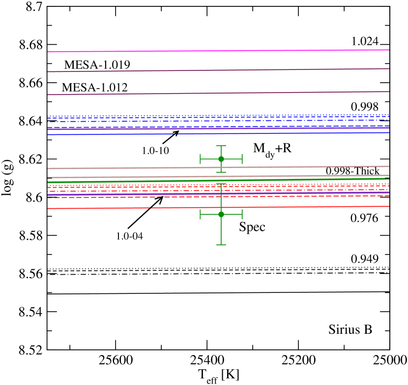
Figure 10: Location of Sirius B in the $T_{\rm eff}-\log g$ plane, using the spectroscopic determinations (Spec) and the dynamical mass combined with the radius (M_dy+R) from Bond et al. (2017a). The lines correspond to theoretical white dwarf sequences, that are color-coded in stellar mass: black lines for $0.949M_{\odot}$, red lines for $0.976M_{\odot}$, blue lines for $0.998M_{\odot}$ and magenta lines for $1.024M_{\odot}$. Solid lines correspond to canonical sequences. Thinner envelopes are depicted with different lines, being thinner as the $\log g$ increases. The violet lines correspond to the cooling tracks from Fontaine et al. (2001) for a stellar mass of $1.0M_{\odot}$ with thick (1.0-04) and thin (1.0-10) hydrogen envelopes. Just for comparison, we included two tracks computed with the MESA code with stellar masses 1.012 and 1.019 $M_{\odot}$ from Lauffer et al. (2018). The thick brown line labelled "0.998-Thick" correspond to a cooling track computed with LPCODE having thicker hydrogen envelopes than the canonical value (see text for details).

.

Note that, the uncertainties associated to the spectroscopic determinations of the atmospheric parameters in the literature correspond to internal errors and could be as large as 1.2 % in effective temperature, and 0.038 dex in $\log g$ (Barstow et al., 2005; Liebert et al., 2005). In the case of Sirius B, Joyce et al. (2018a) computed the atmospheric parameters using different spectra for HST and found a dispersion for $\log g$ of 0.05 dex, leading to spectroscopic stellar masses between 0.874 and 0.962 $M_{\odot}$. With this criteria, the uncertainties in the spectroscopic mass are three times larger than the ones considered by Bond et al. (2017a). In addition, the uncertainties presented by Bond et al. (2017a) correspond to uncorrelated internal uncertainties of the fitting, even though the orbital parameters and stellar masses are correlated. By computing the uncertainties using a simple error propagation statistics, we obtain an uncertainty $\sim 48$% larger for the mass of Sirius B, implying that the quoted uncertainties could be underestimated.

In Figure 11 we compare the observational parameters for Sirius B with our theoretical models using the mass–radius relation. The different lines correspond to theoretical mass–radius relations for an effective temperature of $T_{\rm eff}=25\,369$ K. The solid black line corresponds to the sequences with the thickest hydrogen envelope allowed by single stellar evolution, computed with LPCODE, while the solid magenta line correspond to the thinnest envelope, with $M_{\rm H}\sim 10^{-9.33}M_{*}$. We also show the theoretical mass–radius relation from Fontaine et al. (2001) with hydrogen envelope mass $M_{\rm H}\sim 10^{-4}M_{*}$ as a dashed line. We include the gravitational redshift mass from Joyce et al. (2018b) obtained using parallaxes from Hiparcos (full triangle) and Gaia DR2 (open triangle), from Bond et al. (2017a) (full square) and from Barstow et al. (2005) (red diamond). With a black circle, we show the result obtained by considering the spectroscopic mass computed in this work combined with the radius from Joyce et al. (2018b).

Figure 11: Same as figure 9 but for Sirius B and an effective temperature of $T_{\rm eff}=25\,369$ K. The points show the location of the spectroscopic mass obtain in this work combined with the radius from Joyce et al. (2018b) (circle), the dynamical mass from Bond et al. (2017a) (square) and the gravitational redshift mass from Joyce et al. (2018b) considering parallax from Hipparcos (full triangle) and Gaia DR2 (open triangle).

As expected, the spectroscopic mass and the dynamical mass from Bond et al. (2017a) do not agree within the uncertainties in 1 $\sigma$. However, the results from Joyce et al. (2018b) are compatible with our theoretical mass – radius relation, within 1 $\sigma$ for a hydrogen envelope with $M_{H}\sim 2\times 10^{-6}M_{*}$. Note that, the mass and radius for Sirius B from Joyce et al. (2018b) are also in agreement with the “thick” envelope, with $M_{H}=10^{-4}M_{*}$, sequences from (Fontaine et al., 2001).

A thicker envelope could perhaps be expected if Sirius B had accretion episodes after the residual nuclear burning has turned off. Considering that the Sirius system is a visual binary with a period of $\sim 50$ yr (Bond et al., 2017a), this scenario can be disregarded. The accretion rate of hydrogen from the interstellar medium is less than $10^{-17}M_{\odot}$/yr (Dupuis et al., 1993; Koester & Kepler, 2015), too low to build a thick hydrogen envelope of $\sim 10^{-4}M_{*}$. In any case, as it was shown in section 3.1, the increase of the hydrogen content will trigger nuclear burning at the base of the envelope, reducing the hydrogen mass to $\sim 10^{-6}M_{*}$.

Davis et al. (2011) determined the structure parameters for Sirius A using photometry and spectroscopy combined with parallax, to be $R=1.7144\pm 0.009R_{\odot}$, $T=9845\pm 64$ K and $L=24.74\pm 0.70L_{\odot}$. Considering the uncertainties in mass and metallicity, we estimate an age between $205-245$ Myr. With a cooling age of $115\pm 6$ Myr, the stellar mass of the progenitor of Sirius B is $5.11^{+0.47}_{-0.28}M_{\odot}$, in agreement with the value obtained by Bond et al. (2017a) and Liebert et al. (2005).

5.1.3 Binaries with non-DA white dwarf components

In this section we briefly consider two non-DA white dwarfs in binary systems: Procyon B and Stein 2051 B. Procyon B is a DQZ white dwarf with an effective temperature of $7740\pm 50$ K (Provencal et al., 2002) in a binary system with a slightly evolved subgiant of spectral type F5 IV-V. The Procyon system was analysed by Bond et al. (2015) using precise relative astrometry for HST observations combined with ground base observations and parallax. For Procyon B, the dynamical mass resulted in $M_{*}=0.593\pm 0.006M_{\odot}$ and the radius, determined using flux and parallax measurements, was $0.01232\pm 0.00032R_{\odot}$.

Stein 2051 B, is a DC white dwarf with $T_{\rm eff}=7122\pm 181$ K, in a binary system with a main sequence companion of spectral type M4. The stellar mass was determined by Sahu et al. (2017) using astrometric microlensing, being $M=0.75\pm 0.051M_{\odot}$, while the radius of $R_{*}=0.0114\pm 0.0004R_{\odot}$ was determine using photometry and parallax measurements.

Figure 12 shows the position of Procyon B and Stein 2051 B as compared to the theoretical mass–radius relations for $T_{\rm eff}=7450$ K. The red point-dashed line corresponds to thin hydrogen envelope models, with $M_{H}=10^{-9}M_{*}$ while the green dashed line corresponds to DB white dwarf models from Althaus et al. (2009). We also included the mass-radius relation for thick envelope models computed with LPCODE, those with the thickest hydrogen envelope allowed by stellar evolution. Considering the uncertainties reported by Bond et al. (2015), Procyon B is in very good agreement with our theoretical models for thin H-envelope, as it was found by Bond et al. (2015, 2017b), but also is in agreement with the theoretical mass–radius relation for DB white dwarfs. The results for Stein 2051 B are not that conclusive since the uncertainties are too large, but are still consistent with the theoretical models.

Figure 12: Same as figure 9 but for the non-DA white dwarfs Procyon B and Stein 2051 B, where the observations are those from Bond et al. (2015) and Sahu et al. (2017), respectively. The curves are the mass–radius relation for an effective temperature $T_{\rm eff}=7450$ K, for thick (solid balck line) and thin ($M_{H}=10^{-9}M_{*}$, red point-dashed line) and DB white dwarf models from Althaus et al. (2009) (green dashed line).

5.2 Eclipsing binaries

Figure 13: The white dwarf Mass-Radius relation. Solid lines correspond to thick envelope models, while dashed lines correspond to sequences with $M_{H}/M_{*}=10^{-10}$. From top to bottom, the solid lines are color coded, corresponding to effective temperatures of $60\,000$ K (black), $50\,000$ K (blue), $40\,000$ K (red), $30\,000$ K (green), $20\,000$ K (violet), $10\,000$ K (orange). The data point are the sample extracted from Parsons et al. (2017) and indicated with different symbols that are color coded as well.

Parsons et al. (2017) presented mass and radius determinations for 16 white dwarfs in detached eclipsing binaries with low mass main sequence stars companions and combined them with 10 previous measurements to test the theoretical mass–radius relation. The mass and radius are estimated from the eclipses and radial velocity measurements, while the effective temperature of the white dwarf component is determine using spectroscopy. We selected the objects with stellar masses larger than $\sim 0.5M_{\odot}$, that are covered by our model grid. The selected sample is depicted in figure 13, were we compare the observations extracted from Parsons et al. (2017) to the theoretical mass–radius relation. The solid (dashed) lines correspond to the theoretical mass–radius relations for canonical ($M_{H}/M_{\odot}=10^{-10}$) models for effective temperatures from $60\,000$ K to $10\,000$ K, from top to bottom, in steps of $10\,000$ K (see figure for details). From this figure we see a very good agreement between models and observations, being also consistent in effective temperature.

Table 4: White dwarf stars in detached eclipsing binaries analysed in figure 14. For each object we list the effective temperature, stellar mass and radius (columns 2, 3 and 4) from Parsons et al. (2017) and the hydrogen envelope mass determined in this work.

obj ID	$T_{\rm eff}(K)$	$M(M_{\odot})$	$R(R_{\odot})$	$M_{H}/M_{*}$
CSS 21357	$15909\pm 285$	$0.6579\pm 0.0097$	$0.01221\pm 0.00046$	$5.8\times 10^{-5}-4.6\times 10^{-10}$
GK Vir	$50000\pm 673$	$0.5618\pm 0.0142$	$0.01700\pm 0.00030$	$(1.67\pm 0.30)\times 10^{-4}$
NN Ser	$63000\pm 3000$	$0.5354\pm 0.0117$	$0.02080\pm 0.00020$	$(2.18\pm 0.23)\times 10^{-4}$
QS Vir	$14220\pm 350$	$0.7816\pm 0.0130$	$0.01068\pm 0.00007$	$1.8\times 10^{-5}-4.6\times 10^{-10}$
J0024+1745	$8272\pm 580$	$0.5340\pm 0.0090$	$0.01398\pm 0.00070$	$2.2\times 10^{-4}-2.6\times 10^{-10}$
J0138-0016	$3570\pm 100$	$0.5290\pm 0.0100$	$0.01310\pm 0.00030$	$2.3\times 10^{-4}-5.8\times 10^{-10}$
J0314+0206	$46783\pm 7706$	$0.5967\pm 0.0088$	$0.01597\pm 0.00022$	$(1.25\pm 0.01)\times 10^{-4}$
J0121+1744	$10644\pm 1721$	$0.5338\pm 0.0038$	$0.01401\pm 0.00032$	$(2.21\pm 0.73)\times 10^{-4}$
J1123-1155	$10210\pm 87$	$0.6050\pm 0.0079$	$0.01278\pm 0.00037$	$(1.02\pm 0.10)\times 10^{-4}$
J1307+2156	$8500\pm 500$	$0.6098\pm 0.0031$	$0.01207\pm 0.00061$	$9.6\times 10^{-5}-1.4\times 10^{-10}$
V471 Tau	$34500\pm 1000$	$0.8400\pm 0.0500$	$0.01070\pm 0.00070$	$9.8\times 10^{-6}-4.8\times 10^{-10}$

Next we proceed to measure the hydrogen content in the selected sample of eleven white dwarfs. The sample is listed in table LABEL:parson17-table, along with the effective temperature, stellar mass and radius extracted from Parsons et al. (2017). For each object we compare the observed mass and radius with our theoretical mass–radius relation, considering different thickness of the hydrogen envelope. From the selected sample, only five objects, GK Vir, NN Ser, J0138-0016, J0121+1744 and J1123-1155, show uncertainties small enough to measure the hydrogen envelope mass, within our model grid. The remaining objects are consistent with the theoretical mass–radius relation but the uncertainties are too large to constrain the mass of the hydrogen content. The results for the five objects are depicted in figure 14, while the values for the hydrogen envelopes are listed in the last column of table LABEL:parson17-table. From figure 14 it shows that all five objects have a canonical hydrogen envelope, i,e., the maximum amount of hydrogen as predicted by stellar evolution theory. This is expected given the mass range of the objects, for which the hydrogen envelope is intrinsically thicker. Also, note that the larger differences between the theoretical mass–radius relations for different hydrogen envelope mass occurs for low stellar masses and higher effective temperatures, as shown in figure 6.

Figure 14: Comparision with the observational values for mass and radius for five white dwarf in eclipsing binaries presented in Parsons et al. (2017), with the theoretical mass-radius relations for different masses of the hydrogen envelope. Each panel corresponds to a single object. The hydrogen envelope for each curve is color-coded (see inset in the figure).

6 Conclusions

In this work we studied the mass–radius relation for white dwarf stars and its dependence with the hydrogen envelope mass. In particular, how the extension of the hydrogen envelope affects the radius, and the surface gravity, which directly impacts the calculation of the stellar mass using atmospheric parameters, i.e., the spectroscopic mass.

We find that, comparing the sequences with the thickest envelope with those having the thinnest hydrogen envelope in our model grid, the reduction in the radius is around 8-12%, 5-8% and 1-2% for stellar masses of 0.493 $M_{\odot}$, 0.609 $M_{\odot}$ and 0.998 $M_{\odot}$, respectively. As expected the differences are larger for models with lower stellar mass since, for these objects, the maximum hydrogen envelope left on top of a white dwarf star is thicker, according to single stellar evolution theory. The reduction of the stellar radius translates directly into an increase in $\log g$ for a fixed stellar mass, that can reach up to 0.11 dex, for low mass and high effective temperatures. Considering that the mean uncertainty in $\log g$ is 0.038 dex, then it is possible to measure the hydrogen envelope mass.

In addition, the maximum hydrogen mass allowed by stellar evolution theory is mass dependent, being thinner than $M_{H}=10^{-4}M_{*}$, for white dwarf masses larger than $0.6M_{\odot}$, and thicker for masses below $0.6M_{\odot}$. Thus, considering a hydrogen envelope of $M_{H}=10^{-4}M_{*}$ for all stellar masses, can lead to overestimated or underestimated spectroscopic masses.

The hydrogen envelope mass is the dominant factor influencing the value of the radius. The central composition leads to less than 1% difference in the radius, as shown by Tremblay et al. (2017). For the helium content, the radius can be reduced by $\sim 1.1\%$ if the helium mass is reduced by more than a factor of 10.

We also use the mass–radius relation as a tool to measure the mass of the hydrogen envelope. We analyse a sample of white dwarf in astrometric and eclipsing binaries, for which it is possible to determine the mass and radius independently of the theoretical models. We consider four white dwarfs in astrometric binaries with very well determined orbital parameters and a sample of eleven white dwarf stars in detached eclipsing binary systems. Our main results are the following.

• For 40 Eridani B, we find a spectroscopic mass of $(0.573\pm 0.0011)M_{\odot}$ and a hydrogen envelope mass of $M_{H}\sim 2.63\times 10^{-8}M_{\odot}$. This result is in agreement with previous determinations, pointing to a thin hydrogen envelope solution. The cooling age for 40 Eridani B is $\sim 145$ Myr, with a total age of $2.68\pm 0.43$ Gyr and a progenitor mass of $1.53\pm 0.11M_{\odot}$.

• For Sirius B, we find a spectrocopic stellar mass of $(0.974\pm 0.013M_{\odot}$ in agreement with previous determinations (Barstow et al., 2005). In addition, the gravitational redshift mass from Joyce et al. (2018b) as compared with our theoretical mass–radius relation, are in agreement within 1 $\sigma$, considering a thick hydrogen envelope of $M_{H}=2.02\times 10^{-6}$. The cooling age for Sirius B is $115\pm 6$ Myr, leading to a stellar mass of the progenitor of $5.11^{+0.47}_{-0.28}M_{\odot}$. As compared to the dynamical mass, the spectrocopic value is 4.3% lower than that obtained by Bond et al. (2017a), and not compatible within the uncertainties. We conclude that, either the uncertainties in the dynamical mass are underestimated by at least $\sim$ 50% or the difference is due to the fitting method and/or current atmospheric models.

• Observations of both non-DA white dwarfs, Procyon B and Stein 2051 B, are consistent with a thin hydrogen envelope ($M_{H}\lesssim 10^{-9}$) as found by Bond et al. (2017b), but also with the pure He theoretical models from Althaus et al. (2009).

• For a sample of 11 white dwarfs in detached eclipsing binaries we found a good agreement between the theoretical mass–radius relation and the observations. For five objects, in the low mass range ($\lesssim 0.6M_{\odot}$), we measured the hydrogen mass and found thick hydrogen envelopes in all cases. For the remaining objects the uncertainties are too large to constrain the hydrogen envelope mass, but the observations are in agreement with the theoretical mass–radius relation.

In general the mass–radius relation computed using our models is in good agreement with the observations. For some objects we were able to constrain the hydrogen envelope mass given the lower uncertainties in the observed mass and radius. However, for most objects uncertainties are still too large. High mass white dwarf models show that these stars are born with hydrogen envelopes of $\sim 10^{-6}M_{*}$ or thinner. Thus the challenge of constrain the hydrogen mass is higher since the difference in radius is 1-2% within the hydrogen mass range allowed by our model grid.

Finally, we emphasize that the maximum hydrogen content left on top of a white dwarf is mass dependent, when the evolution of the white dwarf progenitor in computed consistently. In particular, the hydrogen envelope is thinner than the canonical value for stellar masses larger than $0.6M_{\odot}$ and thicker for stellar masses below that value. Not taking into account this dependence can lead to a overestimation of the stellar mass when the determination is based on spectroscopy, i.e., using the atmospheric parameters $\log g$ and effective temperature.

References

- Alexander & Ferguson (1994) Alexander, D. R., & Ferguson, J. W. 1994, ApJ, 437, 879
- Althaus et al. (2003) Althaus, L. G., Serenelli, A. M., Córsico, A. H., & Montgomery, M. H. 2003, A&A, 404, 593
- Althaus et al. (2005) Althaus, L. G., Serenelli, A. M., Panei, J. A., et al. 2005, A&A, 435, 631
- Althaus et al. (2009) Althaus, L. G., Panei, J. A., Miller Bertolami, M. M., et al. 2009, ApJ, 704, 1605
- Althaus et al. (2010) Althaus, L. G., Córsico, A. H., Bischoff-Kim, A., et al. 2010, ApJ, 717, 897
- Althaus et al. (2013) Althaus, L. G., Miller Bertolami, M. M., & Córsico, A. H. 2013, A&A, 557, A19
- Althaus et al. (2015) Althaus, L. G., Camisassa, M. E., Miller Bertolami, M. M., Córsico, A. H., & García-Berro, E. 2015, A&A, 576, A9
- Barstow et al. (2005) Barstow, M. A., Bond, H. E., Holberg, J. B., et al. 2005, MNRAS, 362, 1134
- Bédard et al. (2017) Bédard, A., Bergeron, P., & Fontaine, G. 2017, ApJ, 848, 11
- Bergeron et al. (2001) Bergeron, P., Leggett, S. K., & Ruiz, M. T. 2001, ApJS, 133, 413
- Bond et al. (2015) Bond, H. E., Gilliland, R. L., Schaefer, G. H., et al. 2015, ApJ, 813, 106
- Bond et al. (2017a) Bond, H. E., Schaefer, G. H., Gilliland, R. L., et al. 2017a, ApJ, 840, 70
- Bond et al. (2017b) Bond, H. E., Bergeron, P., & Bédard, A. 2017b, ApJ, 848, 16
- Burgers (1969) Burgers, J. M. 1969, Flow Equations for Composite Gases, New York: Academic Press, 1969,
- Cassisi et al. (2007) Cassisi, S., Potekhin, A. Y., Pietrinferni, A., Catelan, M., & Salaris, M. 2007, ApJ, 661, 1094
- Castanheira & Kepler (2009) Castanheira, B. G., & Kepler, S. O. 2009, MNRAS, 396, 1709
- Catalán et al. (2008) Catalán, S., Isern, J., García-Berro, E., & Ribas, I. 2008, MNRAS, 387, 1693
- Cummings et al. (2016) Cummings, J. D., Kalirai, J. S., Tremblay, P.-E., & Ramirez-Ruiz, E. 2016, ApJ, 818, 84
- Davis et al. (2011) Davis, J., Ireland, M. J., North, J. R., et al. 2011, Publ. Astron. Soc. Australia, 28, 58
- De Gerónimo et al. (2017) De Gerónimo, F. C., Althaus, L. G., Córsico, A. H., Romero, A. D., & Kepler, S. O. 2017, A&A, 599, A21
- De Gerónimo et al. (2018) De Gerónimo, F. C., Althaus, L. G., Córsico, A. H., Romero, A. D., & Kepler, S. O. 2018, A&A, 613, A46
- Dupuis et al. (1993) Dupuis, J., Fontaine, G., Pelletier, C., & Wesemael, F. 1993, ApJS, 84, 73
- El-Badry et al. (2018) El-Badry, K., Rix, H.-W., & Weisz, D. R. 2018, ApJ, 860, L17
- Falcon et al. (2012) Falcon, R. E., Winget, D. E., Montgomery, M. H., & Williams, K. A. 2012, ApJ, 757, 116
- Fontaine et al. (2001) Fontaine, G., Brassard, P., & Bergeron, P. 2001, PASP, 113, 409
- Fontaine & Brassard (2008) Fontaine, G., & Brassard, P. 2008, PASP, 120, 1043
- Garcia-Berro et al. (1988) Garcia-Berro, E., Hernanz, M., Isern, J., & Mochkovitch, R. 1988, Nature, 333, 642
- Gatewood & Gatewood (1978) Gatewood, G. D., & Gatewood, C. V. 1978, ApJ, 225, 191
- Haft et al. (1994) Haft, M., Raffelt, G., & Weiss, A. 1994, ApJ, 425, 222
- Heintz (1974) Heintz, W. D. 1974, AJ, 79, 819
- Herwig et al. (1997) Herwig, F., Bloecker, T., Schoenberner, D., & El Eid, M. 1997, A&A, 324, L81
- Holberg et al. (2012) Holberg, J. B., Oswalt, T. D., & Barstow, M. A. 2012, AJ, 143, 68
- Horowitz et al. (2010) Horowitz, C. J., Schneider, A. S., & Berry, D. K. 2010, Physical Review Letters, 104, 231101
- Iben (1982) Iben, I., Jr. 1982, ApJ, 260, 821
- Iben & Renzini (1983) Iben, I., Jr., & Renzini, A. 1983, ARA&A, 21, 271
- Iben (1984) Iben, I., Jr. 1984, ApJ, 277, 333
- Iben & Tutukov (1984) Iben, I., Jr., & Tutukov, A. V. 1984, ApJ, 282, 615
- Iglesias & Rogers (1996) Iglesias, C. A., & Rogers, F. J. 1996, ApJ, 464, 943
- Istrate et al. (2014) Istrate, A. G., Tauris, T. M., & Langer, N. 2014, A&A, 571, A45
- Itoh et al. (1996) Itoh, N., Hayashi, H., Nishikawa, A., & Kohyama, Y. 1996, ApJS, 102, 411
- Joyce et al. (2018a) Joyce, S. R. G., Barstow, M. A., Casewell, S. L., et al. 2018a, MNRAS, 479, 1612
- Joyce et al. (2018b) Joyce, S. R. G., Barstow, M. A., Holberg, J. B., et al. 2018b, MNRAS, 481, 2361
- Koester et al. (1979) Koester, D., Schulz, H., & Weidemann, V. 1979, A&A, 76, 262
- Koester (2010) Koester, D. 2010, Mem. Soc. Astron. Italiana, 81, 921
- Koester & Kepler (2015) Koester, D., & Kepler, S. O. 2015, A&A, 583, A86
- Lauffer et al. (2018) Lauffer, G. R., Romero, A. D., & Kepler, S. O. 2018, MNRAS, 480, 1547
- Liebert et al. (2005) Liebert, J., Young, P. A., Arnett, D., Holberg, J. B., & Williams, K. A. 2005, ApJ, 630, L69
- Magni & Mazzitelli (1979) Magni, G., & Mazzitelli, I. 1979, A&A, 72, 134
- Mason et al. (2017) Mason, B. D., Hartkopf, W. I., & Miles, K. N. 2017, AJ, 154, 200
- Montgomery & Winget (1999) Montgomery, M. H., & Winget, D. E. 1999, ApJ, 526, 976
- Parsons et al. (2010) Parsons, S. G., Marsh, T. R., Copperwheat, C. M., et al. 2010, MNRAS, 402, 2591
- Parsons et al. (2012a) Parsons, S. G., Gänsicke, B. T., Marsh, T. R., et al. 2012a, MNRAS, 426, 1950
- Parsons et al. (2012b) Parsons, S. G., Marsh, T. R., Gänsicke, B. T., et al. 2012b, MNRAS, 420, 3281
- Parsons et al. (2017) Parsons, S. G., Gänsicke, B. T., Marsh, T. R., et al. 2017, MNRAS, 470, 4473
- Paxton et al. (2011) Paxton, B., Bildsten, L., Dotter, A., et al. 2011, ApJS, 192, 3
- Paxton et al. (2013) Paxton, B., Cantiello, M., Arras, P., et al. 2013, ApJS, 208, 4
- Provencal et al. (1998) Provencal, J. L., Shipman, H. L., Høg, E., & Thejll, P. 1998, ApJ, 494, 759
- Provencal et al. (2002) Provencal, J. L., Shipman, H. L., Koester, D., Wesemael, F., & Bergeron, P. 2002, ApJ, 568, 324
- Rebassa-Mansergas et al. (2007) Rebassa-Mansergas, A., Gänsicke, B. T., Rodríguez-Gil, P., Schreiber, M. R., & Koester, D. 2007, MNRAS, 382, 1377
- Renedo et al. (2010) Renedo, I., Althaus, L. G., Miller Bertolami, M. M., et al. 2010, ApJ, 717, 183
- Romero et al. (2012) Romero, A. D., Córsico, A. H., Althaus, L. G., et al. 2012, MNRAS, 420, 1462
- Romero et al. (2013) Romero, A. D., Kepler, S. O., Córsico, A. H., Althaus, L. G., & Fraga, L. 2013, ApJ, 779, 58
- Romero et al. (2015) Romero, A. D., Campos, F., & Kepler, S. O. 2015, MNRAS, 450, 3708
- Romero et al. (2017) Romero, A. D., Córsico, A. H., Castanheira, B. G., et al. 2017, ApJ, 851, 60
- Sahu et al. (2017) Sahu, K. C., Anderson, J., Casertano, S., et al. 2017, Science, 356, 1046
- Salaris et al. (1997) Salaris, M., Domínguez, I., García-Berro, E., et al. 1997, ApJ, 486, 413
- Salaris et al. (2000) Salaris, M., García-Berro, E., Hernanz, M., Isern, J., & Saumon, D. 2000, ApJ, 544, 1036
- Salaris et al. (2010) Salaris, M., Cassisi, S., Pietrinferni, A., Kowalski, P. M., & Isern, J. 2010, ApJ, 716, 1241
- Schmidt (1996) Schmidt, H. 1996, A&A, 311, 852
- Schröder & Cuntz (2005) Schröder, K.-P., & Cuntz, M. 2005, ApJ, 630, L73
- Segretain et al. (1994) Segretain, L., Chabrier, G., Hernanz, M., et al. 1994, ApJ, 434, 641
- Shipman et al. (1997) Shipman, H. L., Provencal, J. L., Høg, E., & Thejll, P. 1997, ApJ, 488, L43
- Tassoul et al. (1990) Tassoul, M., Fontaine, G., & Winget, D. E. 1990, ApJS, 72, 335
- Tremblay et al. (2017) Tremblay, P.-E., Gentile-Fusillo, N., Raddi, R., et al. 2017, MNRAS, 465, 2849
- Tremblay et al. (2019) Tremblay, P.-E., Cukanovaite, E., Gentile Fusillo, N. P., Cunningham, T., & Hollands, M. A. 2019, MNRAS, 482, 5222
- van Horn (1968) van Horn, H. M. 1968, ApJ, 151, 227
- van Leeuwen (2007) van Leeuwen, F. 2007, A&A, 474, 653
- Vassiliadis & Wood (1993) Vassiliadis, E., & Wood, P. R. 1993, ApJ, 413, 641
- Vauclair et al. (1997) Vauclair, G., Schmidt, H., Koester, D., & Allard, N. 1997, A&A, 325, 1055
- Winget et al. (1987) Winget, D. E., Hansen, C. J., Liebert, J., et al. 1987, ApJ, 315, L77
- Winget et al. (2009) Winget, D. E., Kepler, S. O., Campos, F., et al. 2009, ApJ, 693, L6
- Wood (1995) Wood, M. A. 1995, White Dwarfs, 443, 41