Equilibrium time-correlation functions of the long-range interacting Fermi-Pasta-Ulam model

Abstract

We present a numerical study of dynamical correlations (structure factors) of the long-range generalization of the Fermi-Pasta-Ulam oscillator chain, where the strength of the interaction between two lattice sites decays as a power $\alpha$ of the inverse of their distance. The structure factors at finite energy density display distinct peaks, corresponding to long-wavelength propagating modes, whose dispersion relation is compatible with the predictions of the linear theory. We demonstrate that dynamical scaling holds, with a dynamical exponent $z$ that depends weakly on $\alpha$ in the range $1<\alpha<3$. The lineshapes have a non-trivial functional form and appear somehow independent of $\alpha$. Within the accessible time and size ranges, we also find that the short-range limit is hardly attained even for relatively large values of $\alpha$.

1 Introduction

Statistical mechanics of long-range interacting systems displays many peculiar features like ensembe inequivalence, long-living metastable states and anomalous diffusion of energy [1, 2, 3]. Other unusual effects range from lack of thermalization upon interaction with a single external bath [4] to the presence, in isolated systems, of non-isothermal inhomogeneous stationary states, where the density and the temperature are anticorrelated [5, 6]. From the dynamical point of view, propagation of perturbations can occur with infinite velocities, in a way qualitatively different from the short-range cases [7, 8, 9].
Long-range forces should have yet unexplored effects on energy transport for open systems interacting with external reservoirs. This issue has so far received little attention in the literature [10, 11, 12, 13, 14] with respect to the case of short-range nonlinear, low-dimensional systems. For the latter there is currently a detailed understanding of anomalous transport properties [15, 16, 17, 18, 19], leading to the breakdown of the classical Fourier law. Anomalous heat diffusion amounts to say that random motion of the energy carriers is basically a Lèvy walk [20], a description that accounts for most of the phenomenology [21, 22, 23].
A considerable insight has been obtained by Nonlinear Fluctuating Hydrodynamics (NFH) , whereby long-wavelength fluctuations are described in terms of hydrodynamic modes [24]. In a system with three conserved quantities, like chains of coupled oscillators with momentum conservation, the linear theory would yield two propagating sound modes and one diffusing heat mode, all of the three diffusively broadened. Nonlinear terms can be added and treated within the mode-coupling approximation [25, 26, 24]. This predicts that, at long times, the sound mode correlations satisfy the Kardar-Parisi-Zhang (KPZ) scaling, while the heat mode correlations follow a Lévy-walk scaling. Several positive numerical tests for several models of coupled anharmonic oscillators with three conserved quantities (e.g., the Fermi-Pasta-Ulam chain with periodic boundary conditions) have been reported in the recent literature [27, 28, 29, 30].
A relevant consequence of the above approaches is that models can be classified in dynamical universality classes, mostly determined by the conserved quantities and the coupling among their fluctuations [31]. This entails the idea of dynamical scaling of equilibrium correlation functions and of the corresponding dynamical scaling exponent $z$ (defined below). Thus, it is interesting to investigate for possible universality classes also in the long-range models and seek for deviations from the standard diffusive behavior.
In this paper we investigate how the interaction range exponent determines the scaling properties of equilibrium time-dependent correlations. In the absence of a theoretical background, numerical results can be of guidance for constructing a theory: here we report a series of simulations for the Fermi-Pasta-Ulam model with long-range interaction [32], previously investigated in different variants in the context of relaxation [33], excitation propagation [8, 34] and heat transport [35, 13, 36, 14].
The paper is organized as follows. Section 2 describes the details of the model, while structure factors and their scaling properties are reported in Section 3. The main features associated to the propagation of energy perturbations are discussed in Section 4 together with the dependence of the standard chaos indicator, the maximum Lyapunov exponent, on the range exponent in Section 5. The main results of our study are summarized in Section 6.

2 The Model

We consider a one-dimensional lattice of $N$ particles with periodic boundary conditions, whose dynamics is governed by the long-range Hamiltonian

$$H=\sum_{i=1}^{N}\left[\frac{p_{i}^{2}}{2}+\frac{1}{N_{0}(\alpha,N)}\sum_{j\neq i}^{N}\,c_{ij}(\alpha)V(q_{i}-q_{j})\right]$$ (1)

where $q_{i}(t)$ and $p_{i}(t)$ are canonically conjugated variables (i.e., the displacement with respect to the equilibrium position at the $i$-th lattice site and its associated momentum, respectively) and the function $V$ specifies the interaction potential. The strength of the interaction is controlled by the coupling matrix $c_{ij}(\alpha)=(d_{ij})^{-\alpha}$, where the quantity $d_{ij}$ identifies the shortest distance between sites $i$ and $j$ on a periodic lattice [37, 38], i.e.

$$d_{ij}=\min\{|i-j|,N-|i-j|\}$$ (2)

The real non-negative exponent $\alpha$ is the parameter that controls the interaction range, while $N_{0}(\alpha,N)$ is given by the generalized Kac prescription, that insures the extensivity with $N$ of Hamiltonian (1):

$$N_{0}(\alpha,N)=\frac{2}{N}\sum_{i=1}^{N}\sum_{j\neq i}^{N}c_{ij}(\alpha).$$ (3)

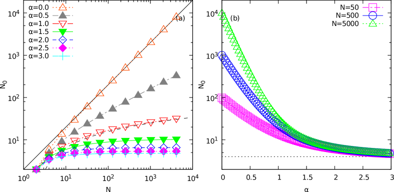
Figure 1: (a) The Kac factor $N_{0}$ as function of the system size $N$. Different sets of points correspond to different values of the exponent $\alpha$ in the range $0\leq\alpha\leq 3$. The solid and the dashed lines draw the linear and the logarithmic trends for $\alpha=0$ and 1, respectively. (b) The Kac factor $N_{0}$ as function of the exponent $\alpha$ for $N=50$ (squares), 500 (circles) and 5000 (triangles). The thin dotted line draws the asymptotic value $N_{0}\to 4$ in the limit $\alpha\to\infty$.

Notice that for $\alpha=0$, i.e. the case of a fully connected lattice, one retrieves the standard Kac prescription, $N_{0}(0)=2(N-1)$. For any finite $\alpha$, $N_{0}(\alpha,N)$ is a monotonically increasing function of $N$: it has a finite positive derivative w.r.t. $N$ for $0<\alpha<1$ ( i.e. in the region where Hamiltonian (1) would be non-extensive in the absence of the Kac factor), while in the large $N$ limit it converges to a constant for $\alpha>1$. The case $\alpha=1$ identifies the extensivity threshold in $d=1$ and $N_{0}(1,N)$ is characterized by a logarithmic divergence with $N$. Finally, in the limit of $\alpha\to+\infty$ one obtains $N_{0}=4$ and $c_{ij}$ vanishes for $|i-j|>1$, while $c_{ij}=1$ for $|i-j|=1$, thus retrieving the case of nearest-neighbor interactions. All this information is summarized in the two panels of Fig. 1.

In this paper, we focus on the Fermi-Pasta-Ulam-$\beta$ (FPU) potential

$$V(x)=\frac{x^{2}}{2}+\frac{x^{4}}{4},$$ (4)

for which we have assumed fixed dimensionless units, in such a way that the only relevant parameter is the total energy $H=E$, or, equivalently, the energy per particle $e=E/N$. A few results about the model with the addition to $V$ of the cubic term $g|x|^{3}/3$ will be also reported. For $\alpha\to+\infty$ the above model reduces to the standard short-range FPU lattice, that has been extensively studied in the context of heat transport in low-dimensional anharmonic chains [39, 40, 41].

The linear dispersion relation for model Hamiltonian (1) with $V$ given by (4) is obtained by neglecting the quartic term and looking for plane-wave solutions of the form $q_{n}\sim\exp(\imath kn-\imath\Omega_{\alpha}t)$ [33, 42] :

$$\Omega_{\alpha}^{2}(k)=\frac{2}{N_{0}(\alpha)}\sum_{n=1}^{N}\frac{1-\cos kn}{n^{\alpha}}$$ (5)

In what follows we will consider periodic boundary conditions so that the allowed values of the wave number $k$ are integer multiples of $2\pi/N$. Note that, at variance with [33, 42], the generalized Kac factor appears explicitly in the definition of $\Omega_{\alpha}$. An important feature of the linear dispersion relation is that in the small wavenumber limit, $|k|\to 0$, the contribution of the leading term is given by the proportionality relations

$$\Omega_{\alpha}(k)\propto|k|^{\frac{\alpha-1}{2}},\quad\text{for}\quad 1<\alpha<3;\quad\propto|k|,\quad\text{for}\quad\alpha\geq 3.$$ (6)

As a consequence, the group velocity diverges as $|k|^{\frac{\alpha-3}{2}}$ in the first case, while it is finite in the second one. This result can be derived from the continuum limit of the equations of motion, where the long-range harmonic force can be approximated as a fractional derivative of order $(\alpha-1)$ [43].
In the present work we will limit the analysis to the case $\alpha>1$ which is the most relevant to the aim of understanding the effect of the interaction range on heat-transport. In fact, in a previous paper [14] we collected evidence that in the genuine long-range case, $0<\alpha<1$, the mechanism of heat transport is dominated by the interaction of each oscillator with the external reservoirs, while the energy exchanged between oscillators is practically immaterial in the limit of large values of $N$. Conversely, for $\alpha>1$ energy currents need to flow through the whole chain and bulk transport processes become relevant. It is thus important, to assess the type of energy diffusion that occurs there.
Before discussing the main results, we want to comment about the numerical method we have adopted. The forces acting between oscillators have been computed by an algorithm based on the Fast Fourier Transform, akin to the one previously used for similar models [38]. In fact, the form of the long-range potential defined at the beginning of this Section allows to write forces as convolution products. This provides a considerable advantage: the computational cost to compute forces in a chain of $N$ oscillators amounts to ${\mathcal{O}}(N\ln N)$, to be compared with any naive algorithmic implementation, that would demand ${\mathcal{O}}(N^{2})$ operations. The integration of the equations of motion $\dot{p}_{i}=-\partial H/\partial q_{i}$ and $\dot{q}_{i}=\partial H/\partial p_{i}$ has been performed by a 4-th order symplectic algorithm [44] with fixed time step $\delta t=0.01$, that guarantees energy conservation with a relative accuracy of ${\mathcal{O}}(10^{-5})$.

3 Structure factors

In the spirit of the NFH theory, many interesting aspects of the heat transport mechanisms can be investigated by looking at the dynamical scaling of the structure factors associated to different linear modes. To accomplish this task we consider the discrete space-Fourier transform of the particles displacement,

$$\hat{q}({k},t)=\frac{1}{N}\sum_{l=1}^{N}q_{l}(t)\,\exp(-\imath{k}l)$$ (7)

and define the dynamical structure factor $S(k,\omega)$ as the ensemble-averaged modulus squared of the temporal Fourier transform of $\hat{q}({k},t)$:

$$S({k},\omega)=\langle|\hat{q}({k},\omega)|^{2}\rangle.$$ (8)

Here the angular brackets denote an equilibrium average in the microcanonical ensemble characterized by the energy density $e$. It is worth recalling that, according to the Wiener-Khinchin theorem, $S({k},\omega)$ is the Fourier transform of the temporal autocorrelation function of $\hat{q}({k},t)$. In the numerical implementation, the microcanonical equilibrium average can be estimated by evolving the dynamics over a sufficiently large set of independent trajectories. A representative example of the numerical results is shown in Fig.2.

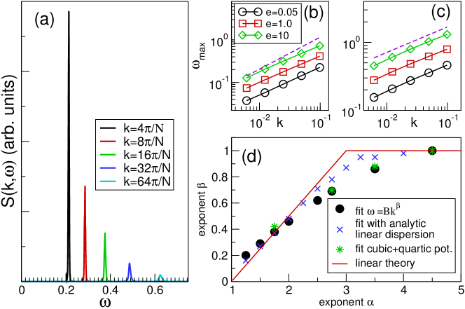
Figure 2: (a) Structure factors of the displacement variable defined in Eq.(8) for the quartic potential, $N=4096$, $\alpha=1.75$, energy density $e=1$ and different values of the wavenumber $k$. Each peak is obtained by averaging over $10^{3}$ independent dynamical trajectories lasting over $10^{4}$ time units. (b,c) Dispersion relations obtained by plotting the peak frequency $\omega_{\rm max}(k)$ as a function of the wavenumber $k$, for $\alpha=1.25$ (b) $\alpha=1.75$ (c) and for different values of the energy density $e$. The dashed lines are the power-law $|k|^{\frac{\alpha-1}{2}}$ predicted by the linear theory (6). (d) The measured exponent $\beta$ versus $\alpha$, see text for details. The solid line corresponds to the scaling given by (6).

In the large-scale limit, i.e. for $k\to 0$, $S(k,\omega)$ exhibits sharp peaks at $\omega=\pm\omega_{\rm max}(k)$ (in panel (a) of Fig.2 we display only the positive $\omega$-axis), that correspond to some kind of propagating modes akin to sound modes usually observed in short-range interacting oscillators [45, 46, 47, 48]. Note that there are no components around $\omega=0$. In the language of NFH this can be an indication that the heat-like mode does not couple significantly with the sound mode.
In order to characterize the nature of these propagating excitations, in Fig.2 (b), (c) and (d) we report an analysis of the positions of the peaks in $k$-space. The figures in panels (b) and (c) show that indeed $\omega_{\rm max}(k)$ scales with a power law $|k|^{\beta}$, with $\beta$ roughly independent of the energy density. In this way one can estimate the value of $\beta$ and report it as a function of the exponent $\alpha$. The full circles in Fig.2 (d) have been obtained in this way. We can see that they are quite close to the predictions of the linear theory (Eq.(6) ), although some sensible deviations are present in the range $2<\alpha<4$. Numerical data can be better fitted by the function $\omega_{\rm max}(k)=B\Omega_{\beta}(k)$ with $\Omega_{\beta}$ given by Eq.(5): $B$ and $\beta$ are the fitting parameters. The estimates of $\beta$ obtained in this way correspond to the crosses in Fig.2 (d), that are closer to the linear scaling (6).
Another interesting observation is that by adding to the interaction potential (4) the cubic term $g|x|^{3}/3$ the dependence of $\beta$ on $\alpha$ does not change significantly (see the stars in Figure 2 (d) ). We want to stress that the data reported have been obtained for $e\sim\mathcal{O}(1)$, where the nonlinear terms of the potential are by no means small with respect to the linear one. This notwithstanding, we obtain evidence that the reasonable agreement of numerical data with the linear dispersion relation accounts, upon a suitable energy-dependent parameter renormalization (by the above defined constant $B$), for a characteristic speed of the excitations, as in the “effective phonon” description used for short-range interacting anharmonic lattices [45].

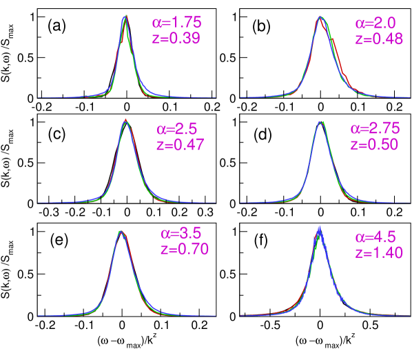
Figure 3: Dynamical scaling of structure factors of displacement for the quartic model $N=2048$, energy density $e=1$ and different values of the range exponent $\alpha$. In each panel four values of the wavenumber ($k=2\pi/N,4\pi/N,16\pi/N,32\pi/N$) are empirically collapsed according to formula (9), the best estimate of the dynamical exponent $z$ is reported alongside. Data are averaged over at least $10^{3}$ trajectories in the microcanonical ensemble.

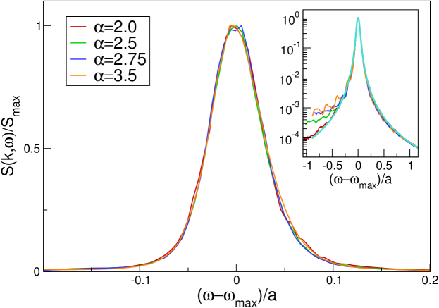
Figure 4: Main panel: Line-shape of structure factors of displacement for the quartic potential; $N=2048$, energy density $e=1$ and fixed $k=16\pi/N$. A data collapse of line-shapes corresponding to different values of the range exponent $\alpha$ is obtained by scaling the horizontal axis by a suitable factor $a$. Inset: the same data plotted in semi-logarithmic scale: the thick cyan solid line is a best fit with a function $A/(B+x^{\eta})$ with $\eta=2.77$.

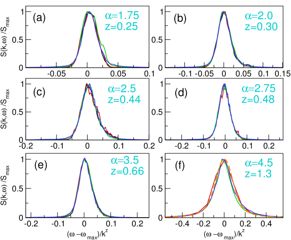
Figure 5: Dynamical scaling of structure factors of displacement for the cubic plus quartic model $N=2048$, energy density $e=1$, $g=0.5$ and different values of the range exponent $\alpha$. In each panel four values of the wavenumber ($k=2\pi/N,4\pi/N,16\pi/N,32\pi/N$) are empirically collapsed according to formula (9), the best estimate of the dynamical exponent $z$ is reported alongside. Data are averaged over at least $10^{3}$ trajectories in the microcanonical ensemble. For comparison in panel (f) we plot the (suitably rescaled) function $f_{KPZ}$ predicted in the short-range case by NFH theory [24] (dashed orange line).

Let us now turn to the issue of dynamical scaling. In analogy with what found in the short-range case, we may surmise that for $\omega\approx\pm\omega_{\rm max}$ structure factors of different wavenumbers $k$ are represented by a suitable scaling function $f_{\alpha}$:

$$S({k},\omega)\sim f_{\alpha}\left(\frac{\omega\pm\omega_{\rm max}}{k^{z}}\right).$$ (9)

In this expression the subscript $\alpha$ points out that, in principle, the kind of scaling function $f$ might depend on $\alpha$. What is expected to depend on $\alpha$ is the dynamical exponent $z$. This is a quantity of major importance, because its value determines the universality class of transport processes. In Fig.3 we illustrate that the above surmise holds independently of $\alpha$. The data have been scaled empirically according to Eq.(9) and the best estimates of $z$ have been determined. The data collapse is generally very good and in some cases excellent.
A further important result is illustrated in Fig.4, where we compare the line-shapes of the structure factors for different values of $\alpha$ at fixed wavenumber $k$ (for the sake of clarity we report just the case $k=16\pi/N$). The line-shapes collapse very well onto each other by suitably rescaling the horizontal axis. Quite remarkably, this indicates that the form of the scaling function $f_{\alpha}$ should be independent of $\alpha$. In the absence of any theoretical hint on its functional form, in the inset of Fig.4 we plot the same data in semi-logarithmic scale, along with an empirical fit. The available data rule out the possibility that the scaling function $f$ could be a simple standard lineshape, like a Gaussian or a Lorentzian one. Fitting rather suggests a non trivial behavior with slowly decaying tails.
For comparison, we also performed a series of simulation for the FPU potential (4) with the addition of the cubic term $g|x|^{3}/3$. The results reported in Fig.5 show that also in this case the scaling hypothesis works quite well in the considered range of values of $\alpha$ and $k$. For this type of potential in the short-range case, the prediction of NFH is $z=3/2$ and the scaling function $f_{\rm KPZ}$ is universal and known exactly [24], albeit not in analytic form, so that one has to compute it numerically [29]. In Fig.5 (f) ($\alpha=4.5$) we plot for comparison also $f_{\rm KPZ}$: it exhibits some systematic deviations from the data-collapsed line-shape, while $z$ is still smaller than the one expected in the short-range limit, $\alpha\to\infty$.

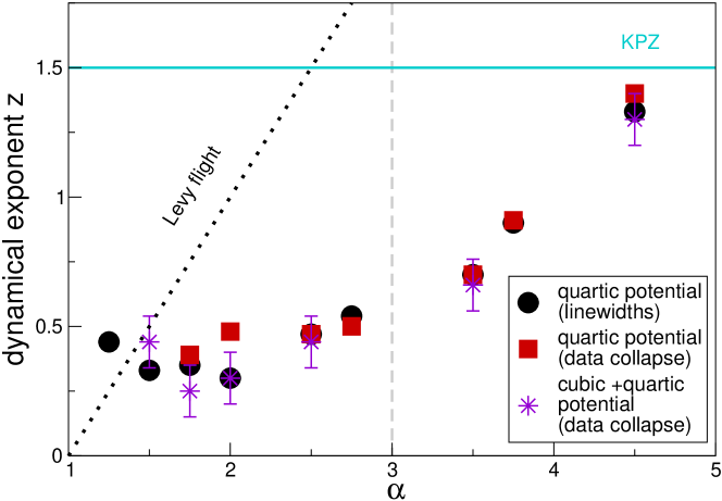
Figure 6: Dynamical exponent $z$ extracted from the measurements of the sound peaks. For comparison, the exponents are measured by data collapse (squares, stars) according to Eq.(9) and by fitting the dependence of line-widths on wavenumber at half maximum by a power law $k^{z}$ (circles). Stars refer to the FPU cubic plus quartic potential. The errors are tentative a priori estimates of the empirical uncertainty in the data-collapse. The grey vertical line signals the value $\alpha=3$ above which the group velocities of linear waves is finite.

The main outcome of our numerical analysis is that we have found evidence that the dynamical exponent $z$ depends on the interaction range exponent $\alpha$ for both the FPU potential (4) and its cubic plus quartic variant. The results are summarized in Fig.6, where, for comparison, we draw the function $z=\alpha-1$, which corresponds to the scaling relation for a simple Lévy flight, i.e. a random walk with step length $\ell$ distributed with probability proportional to $\ell^{-\alpha}$ [49]. The data show that the naive expectation that peak broadening might be described by such simple kinetic process does not account for the observed dependence of $z$ on $\alpha$.
Some further remarks are in order. First of all, for $1<\alpha\lesssim 4$ the dynamical exponent $z$ is smaller than one. At first glance this could appear unusual and unexpected: for instance, think about standard diffusion, where $z=2$. On the other hand, if one considers that the presence of long-range interactions induces instantaneous energy transfer, akin to the dynamical processes characterizing Lévy flights, this fact seems less surprising. Moreover, in the range $1<\alpha<3$, $z$ is weakly dependent on the range exponent $\alpha$, and the numerical data could be also compatible with a constant value, $z\approx 0.4$. Note also that the addition of the cubic term affects very little the value of $z$, the differences being within the uncertainty of the empirical scaling procedure. Finally, for $\alpha>3$ the exponents are remarkably smaller than what predicted for the short-range case within the NFH-mode-coupling approach [24], i.e. $z=3/2$ (horizontal line in Fig.6) and $z=2$ for the cubic plus quartic and pure quartic potentials, respectively. In any case, data seem to indicate that the short-range limit is approached very slowly and, accordingly, we cannot exclude that such a case belongs to a different universality class.

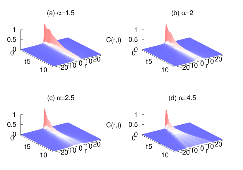
Figure 7: The space-time excess energy correlations $C(r,t)$ for different values of $\alpha$. Simulations have been performed for a chain of $N=1024$ oscillators in a quartic potential with $e=1$.

4 Propagation of energy correlations

The structure factor of the displacement variables $q_{i}(t)$ gives direct information on propagating modes on long spatial and temporal scales. In heat transport problems one is also interested in the propagation of energy fluctuations. Further insight in the energy transport can be obtained by looking at the dynamics of the site energies

$$h_{i}=\frac{p_{i}^{2}}{2}+\frac{1}{N_{0}(\alpha)}\sum_{j\neq i}^{N}\,c_{ij}V(q_{i}-q_{j})$$ (10)

and their (normalized) spatio-temporal correlation functions defined as

$$C(r,t)=\frac{\langle h_{i+r}(t)h_{i}(0)\rangle-\langle h_{i}\rangle^{2}}{\langle h_{i}^{2}\rangle-\langle h_{i}\rangle^{2}}$$ (11)

averaged over the microcanonical ensemble (this is sometimes referred to as excess energy correlation [50, 51]). As usual, translational invariance is assumed, making $C(r,t)$ depend only on the relative distance $r$.
In Fig.7 we compare $C(r,t)$ for different values of $\alpha$. The main outcome is that for $\alpha<3$ energy spreading is somehow slower and propagating peaks of excitation are lacking. We also observed that a similar qualitative behavior characterizes the spreading of an initially localized finite energy perturbation: for instance, this can be checked for a perturbed thermal-equilibrium state, where the kinetic energies of the central 10 oscillators are perturbed (data not shown). This indicates that for $1<\alpha<3$, i.e. in the region of the parameter space where the linear group velocity diverges for small wavenumbers, the model still retains some features of the pure long-range model, where energy can be trapped in single degrees of freedom for arbitrary long times (e.g., see Ref. [8]). We recall that a scaling analysis of the excess energy correlation for the a long-range model with harmonic nearest-neighbor coupling has been presented in Ref.[12]. Although this model has a different harmonic limit (having finite group velocity) there are some resemblance with ours, including the presence of some propagating peaks.

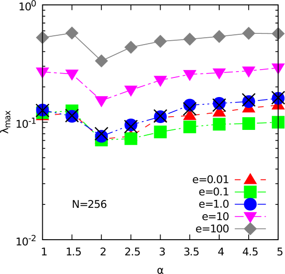
Figure 8: Maximal Lyapunov exponent $\lambda_{\rm max}$ for a long-range quartic FPU chain as function of the range exponent $\alpha$, for $N=256$ and different values of the energy density $e=0.01$ (upward triangles), 0.1 (squares), 1 (circles), 10 (downward triangles) and 100 (diamonds). The heavy crosses mark $\lambda_{\rm max}$ for the cubic plus quartic case with $e=1$.

We also performed some measurements of the energy structure factors $S_{\mathcal{E}}({k},\omega)$, that can be obtained by Fourier-transforming the energy density field defined in Eq.(10) and by computing the modulus squared of its temporal Fourier transform. Here we do not report numerical data, but we just comment that $S_{\mathcal{E}}({k},\omega)$ are characterized by a single central peak, whose width increases with the wavenumber $k$. This is qualitatively consistent with the spreading of the excess energy correlations. Furthermore, a more quantitative analysis has been performed for a couple of values of $\alpha$: within the available frequency range, the data may compatible with dynamical scaling but a reliable estimate of dynamical exponents is not feasible. Also a tentative fitting, suggest that the $S_{\mathcal{E}}$ may have a Lorentzian lineshape, which would imply a Lévy-function shape in real space, analogous to the short-range case [24]. Surely a more quantitative analysis would require very accurate statistical averages and we postpone this task to a future work.

5 Lyapunov exponents

In this last section we complement the above results with an analysis of chaotic properties. Along with previous studies on similar long-range models (see e.g. Refs. [52, 36, 13, 53]) we have computed the maximal Lyapunov exponent $\lambda_{\rm max}$ for $1\leq\alpha\leq 5$ and $64\leq N\leq 16384$, making use of the standard Benettin-Galgani-Strelcyn technique [54]. If on one hand (as expected) $\lambda_{\rm max}$ is essentially constant for increasing $N$ at fixed energy density $e$, on the other hand, for fixed $N$ and for all values of the energy density explored, $\lambda_{\rm max}$ has a remarkably non-monotonic trend with $\alpha$. In particular, it has a relative minimum at $\alpha=2$, as shown in Fig. 8 for $N=256$ and different values of $e$ for the quartic case (filled symbols) and quartic plus cubic case (crosses). We note that, a similar behavior has been reported for the model in Ref. [12], where the quadratic term in (4) is outside the double sum in the model Hamiltonian (1). Interestingly, the $\alpha=2$ case stands out for exhibiting a seemingly ballistic behavior in heat transport [14], that has led to speculate about some sort of (energy dependent) near-integrable behavior or the presence of additional conserved quantities. To assess this possibility we computed also the entire Lyapunov spectra $\lambda_{i}$, $i=1,\ldots,2N$ for $\alpha=2,3,\infty$. The data shown in Fig. 9 demonstrate that the case $\alpha=2$ has the usual four vanishing exponents as the others, corresponding to the usual conservation laws (see the inset of Fig. 9). So the existence of additional integrals of motion should be ruled out. In agreement with this fact, both the scaling analysis of structure factors and the behavior of the space-time excess energy correlations do not display any particular feature to be singled out for $\alpha=2$.

To conclude, let us also mention that the non monotonic behaviour of $\lambda_{\rm max}$ with a control parameter $\alpha$ at fixed energy density $e$ has been observed also for the short-range model obtained by adding to the Toda Hamiltonian a term proportional to $\sum_{i}|q_{i}|^{\alpha}$ (see [55, 56, 57]). In this case however, contrary to what observed here for the long-range FPU chain, such non monotonicity (again with a relative minimum for $\alpha=2$) disappears for increasing values of $e$ at fixed $N$ (see Fig. 2 in [56]), thus pointing towards a different origin of such a non-trivial behaviour of the degree of chaoticity in the two models.

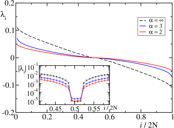
Figure 9: Lyapunov spectra for the long-range quartic FPU chain $\alpha=2,3,\infty$, for $N=64$, energy density $e=1$. The inset reports the absolute values of the exponents zoomed around its minima.

6 Conclusions

In the present work we have undertaken a numerical study of some equilibrium correlations of the long-range FPU model with power-law decaying interaction strengths. In particular, the structure factors of the displacement field provide an interesting complex scenario that we summarize hereafter.

• Even for values of the energy density corresponding to a strongly anharmonic regimes, we obtain convincing evidence of the existence of long-wavelength propagating modes, whose dispersion relation is essentially the one valid for linear waves.

• We obtain also evidence of dynamical scaling, but the corresponding dynamical exponent $z$ depends on the interaction range exponent $\alpha$. In particular, for $1<\alpha\lesssim 4$, $z$ is definitely smaller than one. Lacking any suitable theoretical argument, we cannot envisage any simple relation between these two exponents. Even if it is reasonable to expect that $z$ eventually approaches its value in the short-range case (i.e. in the limit $\alpha\to\infty$), the convergence seems pretty slow.

• Within the numerical accuracy of our simulations, we can conclude that the line-widths of the structure factors are independent of $\alpha$, while any standard Gaussian or Lorentzian form for the scaling function has to be ruled out. Moreover, the similarity between the long-range models of the quartic and of the cubic plus quartic FPU potentials hints at some form of universality in the underlying effective non-linear hydrodynamics. This is a bit surprising, if one considers that these two models, in their short-range version, belong to different universality classes, due to the different symmetries of the forces [58, 24]. Anyway, the previous conjecture demands to be checked for interaction potentials other than the FPU ones – a task that goes beyond the aims of this paper.

• For what concerns the propagation of perturbations in these long-range models we have pointed out that there is a crossover from a localized regime to a propagating one when $\alpha$ increases. A more careful characterization of these two different dynamical phases certainly demands a further numerical effort.

• The case $\alpha=2$ deserves some special consideration. The most puzzling aspect of this case is that different versions of the long-range FPU quartic problem exhibit a sort of “ballistic” transport for $\alpha=2$ (the same value, where $\lambda_{\rm max}$ exhibits a relative minimum). The same peculiar feature does not show up for the cubic plus quartic case (data not shown), despite its overall similarity with the pure quartic one, even with respect to the non-monotonic trend of $\lambda_{\rm max}$ with $\alpha$. On the other hand, the dynamical exponent $z$ measured above is definitely different from one, the value one would expect for ballistic propagation. We do not have an explanation for such apparently contradictory behavior for equilibrium and non-equilibrium, that should be further explored in a future work.

References

References

- [1] Bouchet F, Gupta S and Mukamel D 2010 Physica A: Statistical Mechanics and its Applications 389 4389–4405
- [2] Campa A, Dauxois T and Ruffo S 2009 Phys. Rep. 480 57–159
- [3] Campa A, Dauxois T, Fanelli D and Ruffo S 2014 Physics of long-range interacting systems (OUP Oxford)
- [4] de Buyl P, De Ninno G, Fanelli D, Nardini C, Patelli A, Piazza F and Yamaguchi Y Y 2013 Phys. Rev. E 87(4) 042110
- [5] Teles T N, Gupta S, Di Cintio P and Casetti L 2015 Phys. Rev. E 92 020101 (Preprint 1502.04051)
- [6] Gupta S and Casetti L 2016 New Journal of Physics 18 103051
- [7] Torcini A and Lepri S 1997 Phys. Rev. E 55 R3805
- [8] Pogorelov I V and Kandrup H E 2005 Annals of the New York Academy of Sciences 1045 68 (Preprint nlin/0307004)
- [9] Métivier D, Bachelard R and Kastner M 2014 Phys. Rev. Lett. 112 210601
- [10] Ávila R R, Pereira E and Teixeira D L 2015 Physica A: Statistical Mechanics and its Applications 423 51–60
- [11] Olivares C and Anteneodo C 2016 Phys. Rev. E 94(4) 042117
- [12] Bagchi D 2017 Phys. Rev. E 95 032102
- [13] Bagchi D 2017 Phys. Rev. E 96 042121
- [14] Iubini S, Di Cintio P, Lepri S, Livi R and Casetti L 2018 Phys. Rev. E 97(3) 032102
- [15] Lepri S, Livi R and Politi A 2003 Phys. Rep. 377 1
- [16] Basile G, Delfini L, Lepri S, Livi R, Olla S and Politi A 2007 Eur. Phys J.-Special Topics 151 85–93
- [17] Dhar A 2008 Adv. Phys. 57 457–537
- [18] Iubini S, Lepri S and Politi A 2012 Phys. Rev. E 86 011108
- [19] Lepri S (ed) 2016 Thermal transport in low dimensions: from statistical physics to nanoscale heat transfer (Lect. Notes Phys vol 921) (Springer-Verlag, Berlin Heidelberg)
- [20] Zaburdaev V, Denisov S and Klafter J 2015 Rev. Mod. Phys. 87 483
- [21] Cipriani P, Denisov S and Politi A 2005 Phys. Rev. Lett. 94 244301
- [22] Lepri S and Politi A 2011 Phys. Rev. E 83 030107
- [23] Dhar A, Saito K and Derrida B 2013 Phys. Rev. E 87 010103
- [24] Spohn H 2014 J. Stat. Phys. 154 1191–1227
- [25] Delfini L, Lepri S, Livi R and Politi A 2007 J. Stat. Mech.: Theory and Experiment P02007
- [26] van Beijeren H 2012 Phys. Rev. Lett. 108(18) 180601
- [27] Das S G, Dhar A, Saito K, Mendl C B and Spohn H 2014 Phys. Rev. E 90 012124
- [28] Di Cintio P, Livi R, Bufferand H, Ciraolo G, Lepri S and Straka M J 2015 Phys. Rev. E 92(6) 062108
- [29] Mendl C B and Spohn H 2013 Phys. Rev. Lett. 111(23) 230601
- [30] Cividini J, Kundu A, Miron A and Mukamel D 2017 J. Stat. Mech: Theory Exp. 2017 013203
- [31] Popkov V, Schadschneider A, Schmidt J and Schütz G M 2015 Proceedings of the National Academy of Sciences 112 12645–12650
- [32] Christodoulidi H, Tsallis C and Bountis T 2014 EPL (Europhysics Letters) 108 40006 (Preprint 1405.3528)
- [33] Miloshevich G, Nguenang J P, Dauxois T, Khomeriki R and Ruffo S 2015 Phys. Rev. E 91 032927
- [34] Miloshevich G, Nguenang J P, Dauxois T, Khomeriki R and Ruffo S 2017 J. Phys. A: Math. Theor. 50 12LT02
- [35] Olivares C and Anteneodo C 2016 Physical Review E 94 042117
- [36] Bagchi D 2017 Phys. Rev. E 95 032102
- [37] Gupta S, Campa A and Ruffo S 2012 Physical Review E 86 061130
- [38] Gupta S, Campa A and Ruffo S 2014 Journal of Statistical Mechanics: Theory and Experiment 2014 R08001
- [39] Lepri S, Livi R and Politi A 1997 Phys. Rev. Lett. 78 1896–1899 ISSN 0031-9007
- [40] Lepri S, Livi R and Politi A 2005 CHAOS 15 015118 ISSN 1054-1500
- [41] Wang L and Wang T 2011 EPL (Europhysics Letters) 93 54002
- [42] Chendjou G N B, Nguenang J P, Trombettoni A, Dauxois T, Khomeriki R and Ruffo S 2018 Communications in Nonlinear Science and Numerical Simulation 60 115 – 127 ISSN 1007-5704
- [43] Tarasov V E 2006 Journal of Physics A: Mathematical and General 39 14895
- [44] McLachlan R I and Atela P 1992 Nonlinearity 5 541
- [45] Lepri S 1998 Phys. Rev. E 58 7165–7171
- [46] Lepri S, Sandri P and Politi A 2005 Eur. Phys. J. B 47 549–555
- [47] Gershgorin B, Lvov Y V and Cai D 2005 Phys. Rev. Lett. 95 264302
- [48] Kulkarni M, Huse D A and Spohn H 2015 Phys. Rev. A 92 043612
- [49] Bouchaud J P and Georges A 1990 Phys. Rep. 195 127–293
- [50] Zhao H 2006 Phys. Rev. Lett. 96 140602
- [51] Li Y, Liu S, Li N, Hänggi P and Li B 2015 New J. Phys. 17 043064
- [52] Christodoulidi H, Tsallis C and Bountis T 2014 EPL (Europhysics Letters) 108 40006 (Preprint 1405.3528)
- [53] Christodoulidi H, Bountis A and Drossos L 2018 European Physical Journal Special Topics 227 (Preprint 1801.03282)
- [54] Pikovsky A and Politi A 2016 Lyapunov exponents: a tool to explore complex dynamics (Cambridge University Press)
- [55] Lebowitz J L and Scaramazza J A 2018 arXiv e-prints (Preprint 1801.07153)
- [56] Di Cintio P, Iubini S, Lepri S and Livi R 2018 Chaos Solitons and Fractals 117 249–254 (Preprint 1810.07127)
- [57] Dhar A, Kundu A, Lebowitz J L and Scaramazza J A 2018 arXiv e-prints (Preprint 1812.11770)
- [58] Lepri S, Livi R and Politi A 2003 Phys. Rev. E 68 067102 ISSN 1063-651X