LIMITS ON ELECTROMAGNETIC COUNTERPARTS OF GRAVITATIONAL WAVE-DETECTED BINARY BLACK HOLE MERGERS

Abstract

Unlike mergers of two compact objects containing a neutron star (NS), binary black hole (BBH) mergers are not accompanied by the production of tidally disrupted material, and hence lack the most direct source of accretion to power a jet and generate electromagnetic (EM) radiation. However, following a tentative detection by the Fermi GBM of a $\gamma$-ray counterpart to GW150914, several ideas were proposed for driving a jet and producing EM radiation. If such jets were in fact produced, they would however lack the cocoon emission that makes jets from binary NSs bright also at large viewing angles. Here, via Monte Carlo simulations of a population of BBH mergers with properties consistent with those inferred from the existing LIGO/Virgo observations, and the angular emission characteristic of jets propagating into the interstellar medium, we derive limits on the allowed energetics and Lorentz factors of such jets from EM follow ups to GW-detected BBH merger events to date, and we make predictions which will help tighten these limits with broadband EM follow ups to events in future LIGO/Virgo runs. The condition that $\lesssim 1$ event out of 10 GW-detected BBH mergers be above the Fermi/GBM threshold imposes that any currently allowed emission model has to satisfy the condition $(E_{\rm iso}/10^{49}{\rm erg})(\theta_{\rm jet}/20^{\circ})\lesssim 1$.

1 Introduction

The discovery of gravitational waves (Abbott et al., 2016a) has opened a new window onto the Universe. Furthermore, the simultaneous detection of electromagnetic (EM) radiation from the double binary neutron star merger GW170817 (Abbott et al., 2017a) has demonstrated the impact of these observations in several disparate areas of physics and astrophysics, from high energy astrophysics, to nuclear physics, to cosmology.

The general thinking is that EM radiation accompanying GWs from binary compact object mergers requires at least one of the two objects to be a NS, whose tidally disrupted material provides the accretion energy required to power an electromagnetic counterpart. However, following the first GW detection from a binary BH merger, the GBM detector on the Fermi satellite detected a tentative $\gamma$-ray counterpart, within 1 sec after the GW detection (Connaughton et al., 2016). While this was a low-statistics event, it was of enough interest to spur ideas that could explain such emission, if indeed real. Since there is no accretion material resulting from tidal disruption at merger, various astrophysical scenarios were put forward in which the binary black holes (BBHs) would have some source of pre-existing material, whether related to the progenitor star (Loeb, 2016; Woosley, 2016; Janiuk et al., 2017) and the mini-disk resulting from its supernova explosion (Perna et al., 2016; Murase et al., 2016; de Mink & King, 2017; Martin et al., 2018), or to the environment of the merger, such as an AGN disk (Bartos et al., 2017). Alternatively, the energy source could be entirely of eletromagnetic nature if the BHs are charged (Liebling & Palenzuela, 2016; Zhang, 2016; Liu et al., 2016; Fraschetti, 2018). GRMHD simulations have additionally demonstrated that jets are produced from merging BHs if there is some matter around the BHs at the time of merger (Khan et al., 2018).

The mere possibility that any of the scenarios above (or others) could be realized in nature is very interesting and worth testing. As more GWs from BBH mergers are detected, and EM followups are conducted, the question is what constraints they put to EM emission models. The answer to this question depends on the physical characteristics of the emission (and in particular its geometrical beaming, total energy, Lorentz factor), on the distribution of properties of detected GW events as a function of redshift, and on the observer viewing angle with respect to the emitting jet. An important difference with the case of a double NS merger (or NS-BH for small mass ratios) is that, even if both events were to produce a jet, in the former case the jet would be interacting with the ejecta from the tidally disrupted NS and produce the so-called ’cocoon’ emission, bright at relatively wide angles as observed in GW170817 (Abbott et al., 2017a). On the other hand, in the case of BBH mergers there are no ejecta for any hypothetical jet to interact with, and hence the probability of observing EM radiation off axis is much lower, and dependent on both energy and Lorentz factor of the jet, in addition to the jet size.

In this paper we simulate the evolution of jets expanding into a pure interstellar medium, without any interaction with ejecta from tidally disrupted material. We compute the time-dependent angular emission in $\gamma$-rays (prompt emission) at early times, as well as the longer-wavelength radiation (afterglow) naturally produced by dissipation of the jet into the medium (details in §2). Given the distribution of redshifts and orbital inclinations of BBH mergers as deduced from the GW events observed to date (described in §3), we perform Monte Carlo simulations to predict the fraction of events which would be expected to be above the threshold flux of currently observing instruments in typical observation bands, for a range of jet properties (energy, Lorentz factor, opening angle) (§4). We further derive limits on the presence of jets and their properties (§5) using the available data from the first LIGO run and the EM follow-ups to GW detections. We summarize and conclude in §6.

2 Prompt and afterglow emission from a jet without cocoon

The wide-angle emission, both in the prompt phase and during the afterglow, is computed using the formalism of Lazzati et al. (2017a). Two counter-propagating jets, of energy $E/2$ each, initial Lorentz factor $\Gamma_{0}$, and uniform properties within an angle $\theta_{j}$, propagate into an interstellar medium of density $n$. The prompt emission is computed assuming that the internal energy of the outflow is dissipated at some distance $R_{\rm rad}$ from the engine, and that the duration of the emission lasts for a certain time $t^{\prime}_{\rm eng}$ in the comoving frame of the outflow. The observed bolometric flux is obtained by integrating the local emission over the entire emitting surface, after boosting by the forth power of the Doppler factor $\delta(\Gamma,\theta)=\left[\left(1\,-\,\beta\cos\theta\right)\right]^{-1}$, where $\beta$ is the jet speed in units of the speed of light, and $\theta$ is the angle that the outgoing photon makes with the normal to the jet surface.

For the emission in a specific energy band, we assume a Band spectrum (Band, 1997) with spectral power-law indices $\alpha_{\rm ph}=0$ and $\beta_{\rm ph}=-2.5$, and comoving peak frequency $h\nu^{\prime}_{\rm pk}=2.5$ keV. These gives a typical GRB spectrum (Gruber et al., 2014) with observed peak frequency of 500 keV (for $\Gamma=100$) or an X-ray flash with peak frequency of 50 keV (for $\Gamma=10$). Light curves are calculated by adding up the radiation from three million emission regions, each activated at its own $R_{\rm rad}$, and reaching the observer at a time depending on both the production radius, as well as as the time delay in reaching the observer.

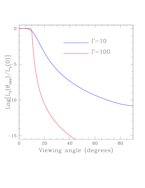
Figure 1: Peak luminosity in the Fermi/GBM band as a function of the observer viewing angle $\theta_{\rm obs}$ with respect to the axis of the closest jet. The function is normalized to its value at $\theta_{\rm obs}=0$, i.e. when the jet is observed on-axis.

For the typical model that we study in this paper (but see later for extensions), we adopt a fiducial value of the jet opening angle of $\theta_{\rm jet}=10^{\circ}$, and explore six different models, produced by the combination of three energy values for the jet, $E=10^{46},10^{47},10^{48}$ ergs and two initial values for the Lorentz factor of the jet, $\Gamma=10,100$. Note that these are the actual energies, which, for the chosen jet angle of $10^{\circ}$, correspond to isotropic energies $\sim 65$ times higher. These isotropic equivalent values straddle the energy inferred for the Fermi/GBM candidate counterpart ($E_{\rm iso}\sim 10^{49}$ ergs). For the Lorentz factor, on the other hand, the two chosen values represent a highly relativistic jet and a mildly relativistic one. Due to relativistic Doppler beaming, the variation of the brightness with viewing angle is very sensitive to the Lorentz factor of the jet, as shown in Fig. 1.

The afterglow radiation, from the X-ray to the radio band, is produced as the jet drives a relativistic shock that propagates and dissipates into the interstellar medium. The local emission is synchrotron radiation (Sari et al., 1998), and the total observed spectrum is computed using a semi-analytic afterglow code (see, e.g., Rossi et al. 2004; Lazzati et al. 2018). The code describes the emission of a relativistic fireball with an arbitrary energy distribution, as seen by observers at arbitrary viewing angles with respect to the jet axis.

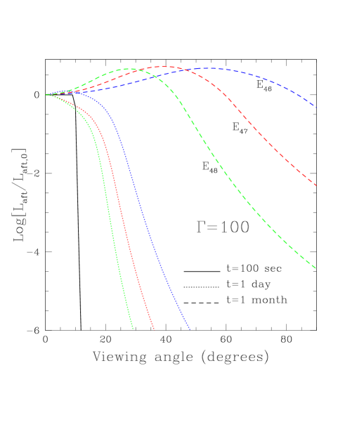
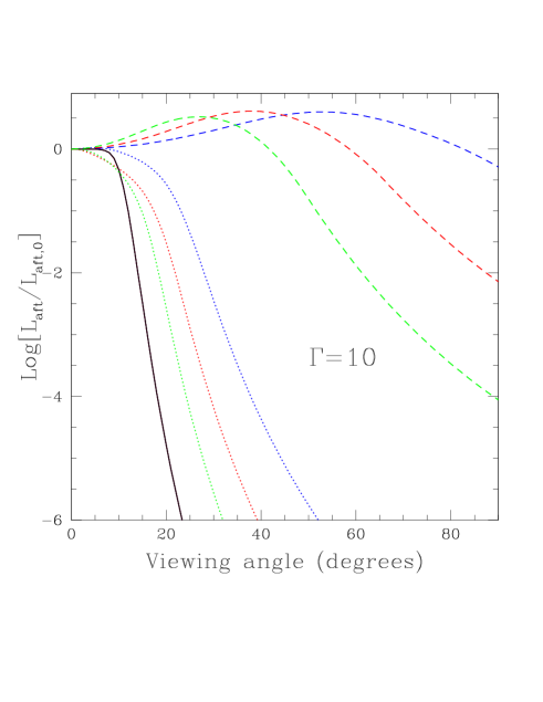
Figure 2: Afterglow luminosity as a function of the observer viewing angle $\theta_{\rm obs}$ with respect to the axis of the closest jet, for three times and the three energy values studied here. In each case, the luminosity function is normalized to its value at $\theta_{\rm obs}=0$, i.e. when the jet is observed on-axis. Note that, while the colors distinguish the three energy values ($E_{46}$ in blue, $E_{47}$ in red, and $E_{48}$ in green), at the two later times (1 day and 1 month), at $t=100$ sec, the (normalized) curves are the same independently of energy, and they are displayed with a single black line for clarity. More energetic jets take a longer time to slow down and hence to isotropize.

In describing the results of our event simulation in §4, we will indicate with the corresponding subscripts the three energy values and the two Lorentz factors, so that, for example, model $E_{47}\Gamma_{10}$ would correspond to the energy $E_{\rm iso}=10^{47}$ ergs, and to the Lorentz factor $\Gamma=10$. Note that the prompt emission scales linearly with energy, and so does the peak of the afterglow emission; however, the afterglow radiation at some specific frequency (or in a given band), does generally not since the break frequencies where the spectrum changes shape depend on energy (Sari et al., 1998). The afterglow intensity further depends on the medium ambient density $n$, as well as on the fraction $\epsilon_{e}$ and $\epsilon_{B}$ of jet energy that goes into the electrons and the magnetic field, respectively, and on the number fraction of accelerated electrons. Inferences of the values of these parameters have been derived via dedicated broadband modeling of the afterglows of gamma-ray bursts. For the astrophysical scenario that we are studying here, the most appropriate sample for comparison is the comprehensive catalogue of 103 short GRBs with prompt follow-up observations in the X-ray, optical, near-infrared and/or radio bands. Fits to the lightcurve of each burst were performed by Fong et al. (2015). Due to the lack of a continuous monitoring in most events, they could not simultaneously fit for all the model parameters, and hence kept fixed the parameter $\epsilon_{e}=0.1$. The magnetic field energy fraction $\epsilon_{B}$ was then found to be consistent with either 0.01 or 0.1 for the greatest majority of the bursts (only a few outliers required smaller values). Since the basic physics of the afterglow phenomenology is expected to be similar for long and short GRBs (it is the result of a point explosion in an external medium), it is useful to look also at results of broadband modeling for long GRBs, which, being typically brighter, generally have a more complete set of broadband data. The sample of well-monitored GRBs modeled by Panaitescu & Kumar (2001) was found to have $\epsilon_{B}$ varying from a few $\times 10^{-5}$ to a few $\times 10^{-1}$, with the largest number of bursts concentrated in the higher range (and those higher values have smaller error bars). The value of $\epsilon_{e}$ was found to be clustered between $\sim 0.01-0.1$. On the other hands, analysis of other bursts by different groups have found lower values; i.e. Wang et al. (2015) found, for a fixed $\epsilon_{e}=0.1$ in their fits, that their sample had $\epsilon_{B}\lesssim 10^{-3}$.

From a theoretical point of view, if the shock simply compresses the upstream magnetic field, then $\epsilon_{B}$ is expected to be low, on the order of $\sim 10^{-7}-10^{-6}$. On the other hand, if the magnetic field is amplified at the shock front via plasma instabilities, then $\epsilon_{B}$ can be as high as $\sim 0.1$ (Medvedev & Loeb, 1999; Nishikawa et al., 2009). In our simulations, we adopt $\epsilon_{e}=0.03$ and $\epsilon_{B}=0.01$. To zeroth order, afterglow luminosities for different values of these parameters can then be derived via analytical scalings (Sari et al., 1998). Following customary habits in afterglow modeling, we further assume that the fraction of electrons which undergo acceleration is on the order of 1. This parameter is hardly constrained by observations, and it is highly degenerate with the other microphysical parameters of the shock (see i.e. discussion in Eichler & Waxman 2005).

The number density, on the other hand, will depend on the type of galaxy and size in which the merger events occur. This (external) variable is expected to vary with the type of progenitors, since merger locations depend on the progenitor type. For BBH mergers, location sites are completely unknown from an observational point of view, at least to date. However, there have been recent numerical (i.e. population synthesis) simulations of isolated binary evolution tracking merger locations (Perna et al., 2018) that can provide a guide. These have shown that, for large galaxies, most of the events will occur in environments with number densities between $\sim 10^{-4}-1$ cm^-3, with generally larger values expected for spiral galaxies and lower for elliptical ones. In our simulations we assume $n=0.01$ cm^-1 as a mean, representative value. However, likewise for the other parameters described above, the luminosities that we derive can be roughly rescaled analytically to different density values, if needed.

The jet size, on the other hand, strongly influences the magnitude of the angular luminosity, which is of fundamental importance for the study carried out here. General relativistic hydrodynamic simulations of accretion flows around black holes remnants of compact object mergers (Aloy et al., 2005) show that ultrarelativistic jets can be driven by thermal energy deposition (possibly due to neutrino-antineutrino annihilation), for energy deposition rates above about $10^{48}$ erg s^-1 and sufficientlhy low baryon density. In those simulations, jets are found to have opening angles $\sim 5^{\circ}-10^{\circ}$, and a sharp edge embedded laterally by a wind with a steeply declining Lorentz factor. Alternatively, jets could be powered via the Blandford-Znajek (BZ) mechanism (Blandford & Znajek, 1977). General relativistic magnetohydrodynamic simulations (Kathirgamaraju et al., 2019) of jets propagating in the environment expected post-merger from a binary neutron star system find a roughly constant Lorentz factor of $\sim 100$ within an angle of about $10^{\circ}$, dropping very rapidly at larger angles. Almost all of the energy is concentrated within $<10^{\circ}$. The luminosity, while also dropping steeply (and becoming $\lesssim 10^{-4}$ of the maximum at viewing angles larger than $\sim 30^{\circ}$), is however shallower than it would have been for a top-hat jet, due to the interaction with the disk-wind. These simulations were however tailored to explain the properties of GRB170817A, resulting from a double neutron star merger, and the jet properties depend on the assumed properties of the disk-wind. For the binary BH case of interest here, Khan et al. (2018) performed general relativistic magneto-hydrodynamic simulations of disk accretion onto black holes with a mass ratio similar to that measured for GW150914. They explored different disk models (in size, scale height), and found that collimated and magnetically dominated outflows emerge in the disk funnel independently of the properties of the disk. The Poynting luminosity is found to converge to the BZ value once quasi-equilibrium is reached. For a fiducial value $\eta=0.1$ of accretion efficiency, they found that an isotropic energy of 1.8$\times 10^{49}$ erg (as inferred for the candidate $\gamma$-ray counterpart to GW150914) can be achieved for a range of disk masses $\sim 10^{-4}-10^{-3}M_{\odot}$, with the specific value depending on the disk model. A fossil disk with mass $\sim 10^{-4}M_{\odot}$ was discussed as a possibility for a dead disk formed from fallback after a supernova explosion (Perna et al., 2016). Hence, at least in theory, the conditions for generating jets from binary black hole mergers do exist. On the other hand, the specific angular dependence of the brightness of such jets will depend on their main driving mechanism, as well as on the structure of the associated disk. Given the above model dependencies, and the fact that bright lateral emission due to the interaction of the jet with ejecta (producing the so-called cocoon and/or a structured jet) is not expected in the binary black hole merger scenario (though there can be weaker off-axis emission due to interaction with a disk-wind), here we adopt the simplest assumption of a top-hat jet with sharp edges. Should any additional emission be present due to disk-wind interaction, this would mostly affect the very large angles in models with high $\Gamma$ and at especially at early times, when $1/\Gamma$ is still small. Hence our results should be intended as the most conservative ones (for the given microphysical parameters) in terms of observability. They will also be the most direct ones to use by observers, when only upper limits to the emission are available.

Fig. 2 shows the afterglow luminosity as a function of the viewing angle at three representative times in the source frame: $t=100$  sec, 1 day, 1 month. The difference between the $\Gamma=100$ (left panel) and the $\Gamma=10$ (right panel) cases is especially apparent at early times, when the fireball has not slowed down yet, and hence the Doppler beaming of the radiation within $1/\Gamma$ causes a sharper decline at viewing angles $\theta_{\rm obs}\gtrsim\theta_{\rm jet}$ for the higher $\Gamma$ case. The behaviour at later times, as a function of the various model parameters, can be readily understood by considering that the fireball starts to decelerate when it has collected an amount of interstellar mass $M_{\rm ISM}\approx E/\Gamma^{2}/c^{2}$. Therefore, for the same energy, the faster fireball will slow down at earlier times than the initially-slower counterpart. On the other hand, for the same initial $\Gamma$, the less energetic is the initial shock, the earlier it slows down and its emission becomes isotropic with viewing angle. Note that, once $\Gamma\sim 1$, the brightness is not uniform with $\theta_{\rm jet}$, as one may naively expect. This is due to the fact that, unlike the prompt emission, which is produced for a thin shell right where the fireball becomes optically thin, the afterglow comes from a large radial region of optically thin material. The radiation that the observer receives depends on both the emission time at location $R_{\rm em}$, as well as on the time for those photons to travel to the observer. For off-axis observers, there is an additional time delay due to the additional path length of the radiation from the edge of the jet closest to the observer, $t_{\rm del}=R_{\rm em}[1-\cos(\theta_{\rm obs}-\theta_{\rm jet})]$, which is longer at larger $\theta_{\rm obs}$. Therefore, emission at larger viewing angles has a contribution from earlier times in the frame of the fireball, when the fireball was brighter. This would explain why there are ranges of viewing geometries for which observers at larger angular distances from the jet axis can measure a brighter emission than observers at smaller angles. For the same initial $\Gamma$, fireballs slow down (and hence isotropize) more quickly for lower jet energies.

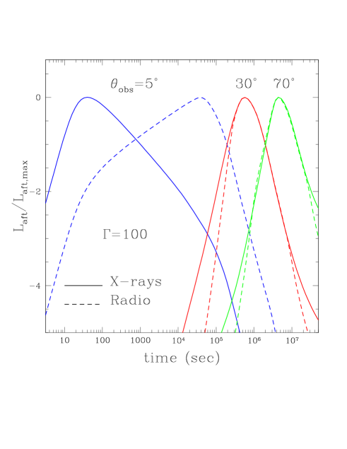
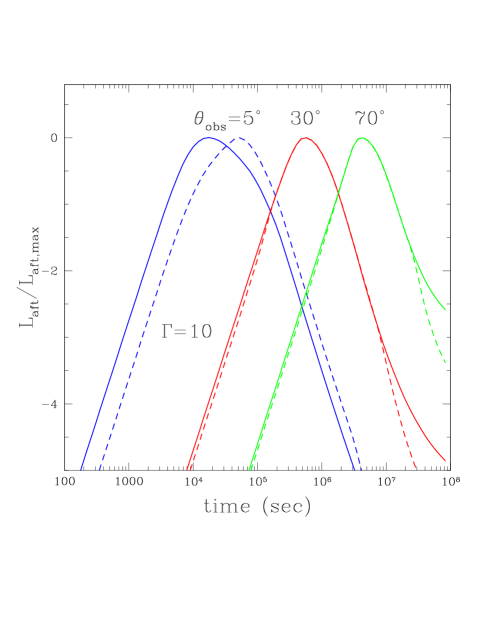
Figure 3: Afterglow luminosity as a function of time, for three viewing angles, two energy bands, and the high and low $\Gamma$ values under study. In all the cases, the jet energy is $E_{\rm 47}$. When all the other parameters are held fixed, the trend with increasing jet energy is of light curves peaking at later times.

The trend of the afterglow luminosity with time is displayed in Fig. 3. For viewing angles larger than $\theta_{\rm jet}$, the rise of the luminosity with time is essentially determined by the viewing geometry, and hence has very little dependence on frequency: as the fireball slows down and the radiation becomes more isotropic, a larger fraction of the jet emission enters into the line of sight. The maximum is reached when the full jet emission reaches the observer, after which it declines following the further slow down and dimming of the jet. On the other hand, for $\theta_{\rm obs}\lesssim\theta_{\rm jet}$, the temporal dependence of the light curve is determined by a combination of factors, and is more strongly dependent on the speed of the fireball, and on the values of the various afterglow parameters ($E,n,\epsilon_{e},\epsilon_{B}$; see Sari et al. 1998). As a result, it also has a much stronger dependence on the frequency of the emission, as can be seen in Fig. 3. For all the other parameters fixed, the general trend with increasing energy (not shown here) is of the peak of the light curve to shift to later times. This is due to the fact that the larger the energy, the longer it takes for the fireball to slow down, and hence for the entire jet to come into the line of view of the observer.

3 Redshift and inclination distribution of the GW-detected BBH mergers

The redshift distribution of the BHs which are detected via their mergers in GWs is just beginning to emerge. Since GWs measure the luminosity distance, they can constrain the redshift dependence of their sources. However, due to the fact that the detection efficiency of GW detectors is a function of the BH masses, the redshift distribution must be fit for simultaneously with that for the BH masses.

This was done by Fishbach et al. (2018) using the data from the first six BBH GW events detected by LIGO: GW150914, LVT151012, GW151226, GW170104, GW170814, and GW170608 (Abbott et al., 2016b, a, c, d, e, 2017b, 2017c). They used the following parameterization for the distribution of the primary and secondary masses in the source frame, $m_{1}$ and $m_{2}<m_{1}$,

$${\cal P}\left(m_{1},m_{2}|\alpha,M_{\rm max}\right)\,\\ =\,A\frac{m_{1}^{-\alpha}}{m_{1}\,-\,M_{\rm min}}{\cal H}\,\left(M_{\rm max}\,-\,{m_{1}}\right)\,{\cal H}\,\left(m_{2}\,-\,M_{\rm min}\right),$$ (1)

where $\cal{H}$ is the Heaviside step function, $A$ a normalization factor, and $M_{\rm min}$ and $M_{\rm max}$ the minimum and maximum BH mass. Conditioned on the mass of the primary, $m_{1}$, the mass of the secondary, $m_{2}$, is drawn from a uniform distribution between $M_{\rm min}$ and $m_{1}$.

For simplicity and to avoid over-parametrization, the mass distribution for both $m_{1}$ and $m_{2}$ was assumed to be redshift-independent (likely a reasonable assumption given the low-redshift of the LIGO horizon), so that the full probability distribution can be written as ${\cal P}(m_{1},m_{2},z)={\cal P}(m_{1},m_{2}){\cal P}(z)$. Fishbach et al. (2018) parameterized the redshift distribution as

$${\cal P}(z)\propto\frac{\mathrm{d}V}{\mathrm{d}z}\left(1+z\right)^{\gamma-1},$$ (2)

where $V$ is the comoving volume (Hogg, 1999); for a merger rate that is uniform in the comoving frame the parameter $\gamma=0$ (the distribution of observed redshifts follows $(1+z)^{\gamma-1}$ due to the redshifting of time between the source and observer frames). A merger rate that tracks the star formation rate at low redshift corresponds to $\gamma\simeq 3$.

Here we choose the parameter values $\alpha=1$ and $\gamma=3$. We fix the minimum mass in Eq. (1 ) to $M_{\rm min}=5\,M_{\odot}$, and the maximum mass $M_{\rm max}=40\,M_{\odot}$. We fix the $z=0$ BBH merger rate to $100\,\mathrm{Gpc}^{-3}\,\mathrm{yr}^{-1}$. To determine which merger events are detected, we use the (semi) analytic selection function described in Abbott et al. (2016c, f), with estimated detector sensitivities taken from Abbott et al. (2018). These choices of parameters are consistent with the inference in Fishbach et al. (2018) and also with the complete set of LIGO observations to date (The LIGO Scientific Collaboration et al., 2018).

For given BH masses and redshifts of the merging binaries, the inclination angle $\theta_{\rm incl}$ that the perpendicular to the orbital plane makes with the observer line of sight is computed according to a probability distribution which is intrinsically isotropic, but weighed by the LIGO sensitivity to detecting GWs for various inclinations.

4 Event statistics from Monte Carlo simulations

We use the distributions in §2 and 3 to generate our event population.

If there is a disk/torus of matter surrounding the merging BBHs, a jet is expected to be launched in the direction perpendicular to its plane (Khan et al. 2018; see also Yamazaki et al. 2016). The next question is then how the plane of the disk is related to the orbital plane of the merging BHs. The simplest and most natural assumption would be of the two planes to be the same, and hence we perform one set of Monte Carlo simulations considering this scenario, which implies $\theta_{\rm obs}$ to be the same as $\theta_{\rm incl}$. However, depending on the source of the matter, this may not necessarily be the case. If, for example, the disk is the remnant of fallback from the SN explosion of one of the two BHs, then its plane would rather be related to the rotation axis of the progenitor star, and hence to the spin of the remnant BH. Therefore, to account for more general and less restrictive astrophysical scenarios, we additionally perform a second set of simulations in which the viewing angle $\theta_{\rm obs}$ with respect to the jet axis is randomly generated on the sky, and independent of $\theta_{\rm incl}$.

Given the redshift of the merger event, and the viewing angle with the jet axis simulated according to either of the scenarios above, the corresponding electromagnetic luminosity in representative bands is then computed as described in §2, and used to calculate the corresponding fluxes at the observer.

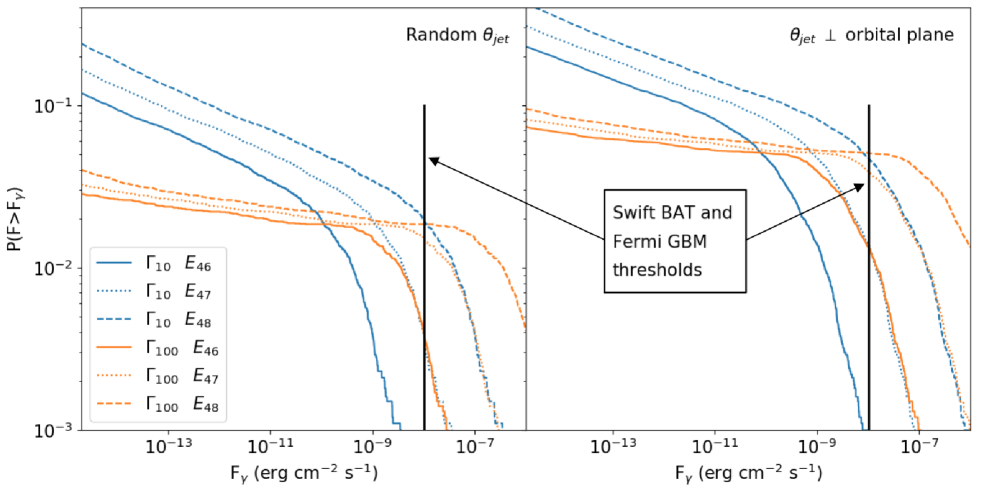
Figure 4: Probability of detecting a $\gamma$-ray signal with flux larger than $F_{\gamma}$ for each of the models studied here: Left: The jetted EM emission is assumed to be uncorrelated with the orbital plane of the BBH prior to merger; Right: The jet axis is assumed to be perpendicular to the orbital plane. The arrow indicates the fraction of events which are above the flux limit of Swift/BAT and Fermi/GBM, before correcting for the limited field of view of each instrument. Note that the BAT and GBM sensitivities are comparable but not exactly the same (see text for specific details).

For each of the six models discussed in §3, we ran $N_{\rm sim}=10^{4}$ realizations. The distribution of peak fluxes in $\gamma$-rays is shown in Fig. 4, both for the model with random $\theta_{\rm jet}$ (left panel), as well as for the one with $\theta_{\rm jet}=\theta_{\rm incl}$ (right panel). The vertical line marks the flux limit of $10^{-8}$ erg s^-1 cm^-2. This roughly corresponds to the sensitivity of Swift/BAT to a typical GRB spectrum. In the case of Fermi/GBM, since the sensitivity is provided in photon counts (and the conversion to fluence requires a spectral assumption), we simply note that the least fluent GRB detected by Fermi has a flux of $2.2\times 10^{-8}$ erg cm^-2 s^-1 (Bhat et al., 2016). This is a bit higher than the Swift threshold, but of the same order of magnitude, which is why for simplicity we indicated the two thresholds with the same line in the figure. Additionally, note that the event detection probabilities at those instrumental sensitivities need to be corrected for the field of view of each instrument (1.4 sr for Swift and 9.5 sr for Fermi).

As expected, the probability is somewhat higher in the case in which the jet producing the EM emission is aligned with the orbital angular momentum of the merging BHs. This is because LIGO has an enhanced detection probability to ’face-on’ events, which in this case would correspond to jets viewed on-axis. Among the models explored here, the probability is larger than $\sim 0.1\%$ except for the $\Gamma_{10}E_{46}$ case and randomly-oriented jet. The maximum probability approaches $\sim 6-7\%$ for the model with the largest energy, $E_{48}$, and jet perpendicular to the orbital plane. The shape of the probability curves is strongly dependent on the fact that, even in mildly relativistic shocks, the brightness is a strong function of the viewing angle (see Fig. 1), since the high energy $\gamma$-rays are expected during the very early times, on a timescale of seconds, when the fireball has not started to slow down yet. Hence, to first order, the main determinant of the probability function for visibility in $\gamma$-rays at low fluxes is the luminosity function of the jet. This is especially so for larger $\Gamma$, when the jet side emission drops very rapidly to negligible levels. This is why the probability curves for the $\Gamma=100$ cases do not increase significantly (and are flatter than those for $\Gamma=10$) at the low flux limits displayed in Fig. 4. The high-flux tail of the probability distribution, on the other hand, is dominated by the bright bursts which are seen face-on. The bright tail hence follows the Euclidean $P(>F_{\gamma})\propto F_{\gamma}^{-3/2}$.

The situation is more complex at longer wavelengths and longer times, as it can be evinced from Fig. 2 and 3. The visibility increases with time at larger angles as the jet decelerates. However, the afterglow luminosity is the brightest at a time which is determined, to first order, by the viewing geometry, but also depends somewhat on the initial $\Gamma$, jet energy, and band (see Fig. 3 and discussion in §3)..

The results of the Monte Carlo simulations for the afterglow in 3 representative bands (X in the 2-10 keV band, Optical at $4.3\times 10^{14}$ Hz and Radio at 1.4 GHz) are summarized in Figs. 5, 6, and 7. For each band, we have also included some reference instrumental detection sensitivities for some of the most common follow-ups in that band. The detection probabilities are time-dependent, and hence they are influenced by the total duration and frequency of the coverage. As such, detailed inferences from a comparison between theory and data can only be made case-by-case. Hence in the following we will draw some general conclusions. For jet energies $\sim 10^{46}$ ergs (corresponding to $E_{\rm iso}\sim 6.5\times 10^{47}$ ergs), the detection probability with current instruments is practically negligible in any band, even if caught around the time at which the emission peaks in that band, The most optimistic scenario studied here is the $\Gamma_{100}E_{48}$ one, with the jet aligned with the orbital angular momentum (right panel of Fig. 7). In all the bands, the detection probabilities turn over at around 3% for observations carried out around the maximum brightness. This is typically achieved at early times, $t_{\rm obs}\lesssim 1$ day.

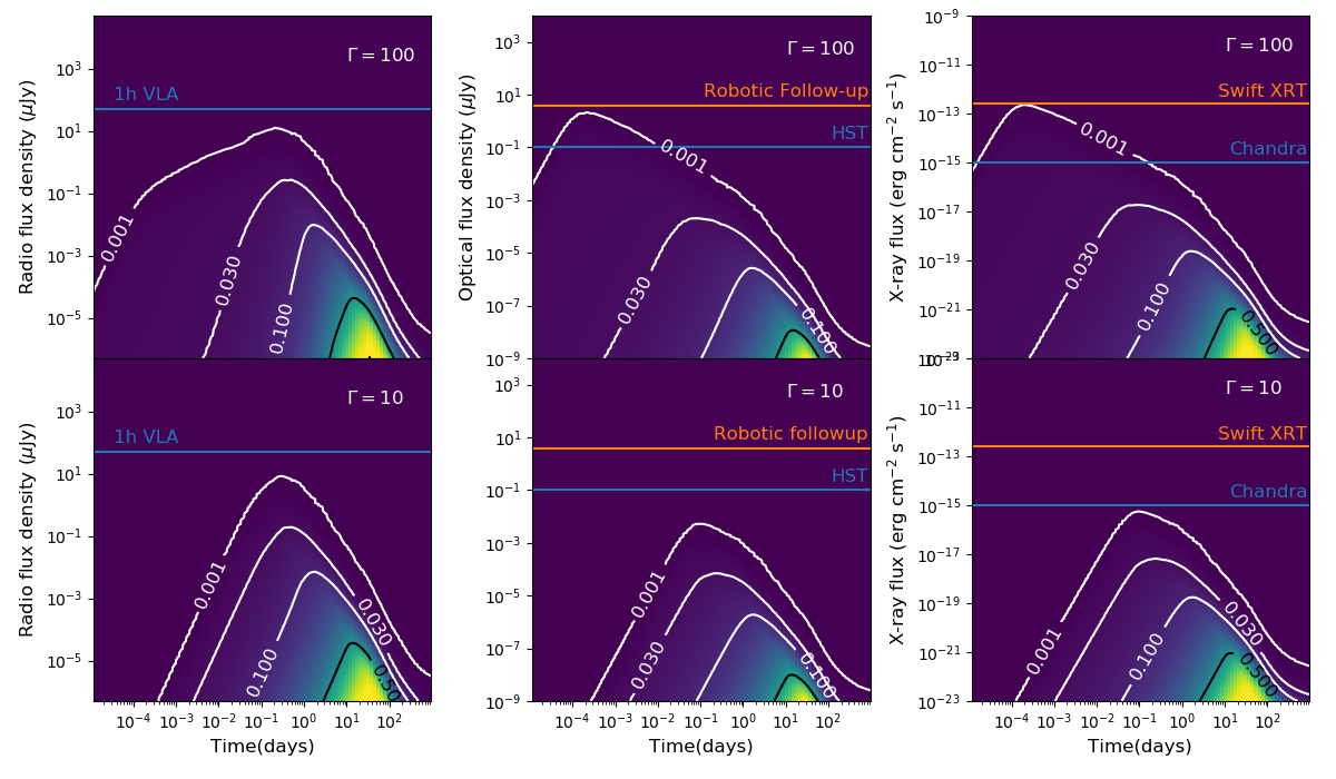
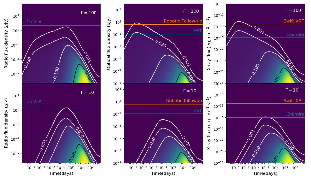
Figure 5: Probability of detecting an EM counterpart in three representative bands (Radio, Optical, X-rays from left to right of each panel), for the model with jet energy $E_{46}$. Left: The jet direction is assumed to be uncorrelated with the orbital plane of the merging BHs. Right: The direction of the jet is assumed to be the same as the one of the orbital angular momentum. Also included in the figure some representative detection limits with current observational facilities. We remind that these probabilities have been computed for a number density of the external medium $n=0.01$ cm^-2, and that the flux scaling goes from $\propto n^{5/14}$ for a fully radiative blastwave to $\propto n^{1/2}$ for a fully adiabatic one. Hence mergers in dense regions can be expected to have significantly higher detection probabilities.

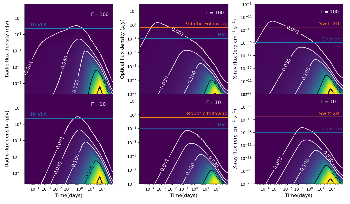
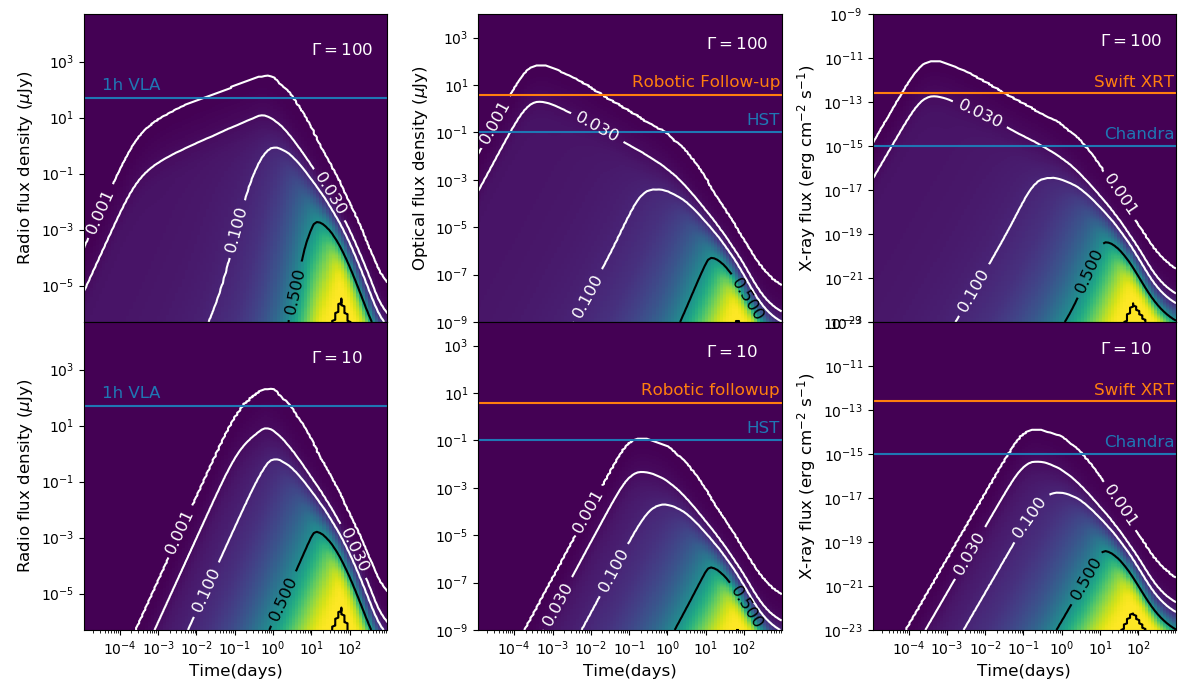
Figure 6: Same as in Fig.5 but for the model with $E_{47}$.

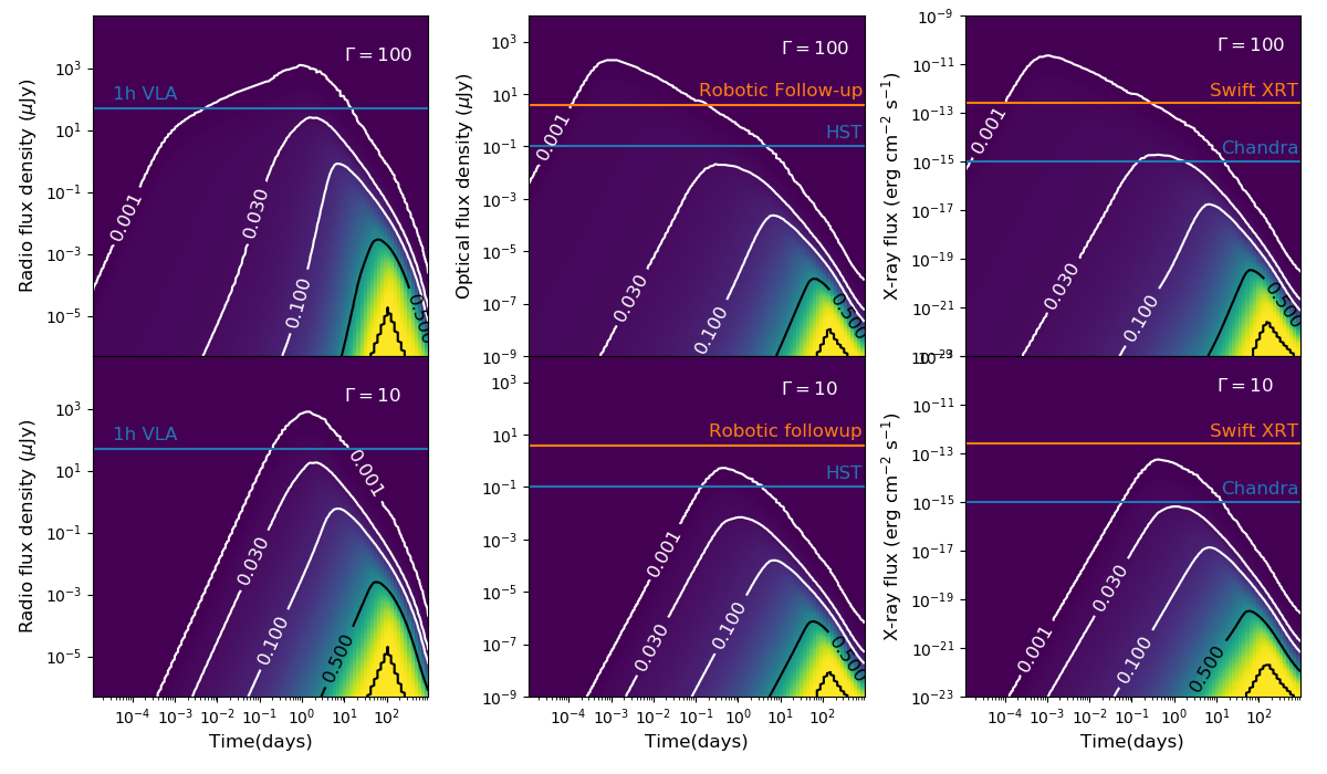
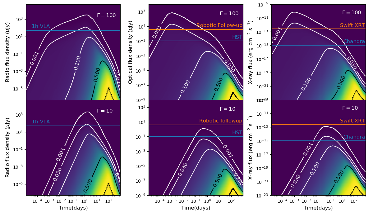
Figure 7: Same as in Fig.5 but for the model with $E_{48}$.

Last, a word of caution in strictly interpreting the probabilities in Figs. 5, 6 and 7. We remind the reader that the afterglow luminosity depends on several microphysical parameters, as well as on the ambient medium density, as discussed in detail in §2. Therefore, each of the curves showed in Figs. 5, 6 and 7 should be interpreted as having a swath of variability for the quoted model parameters.

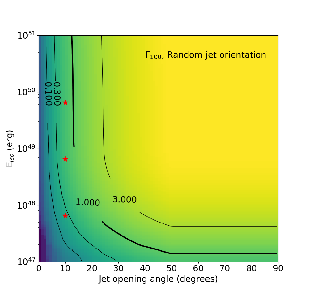
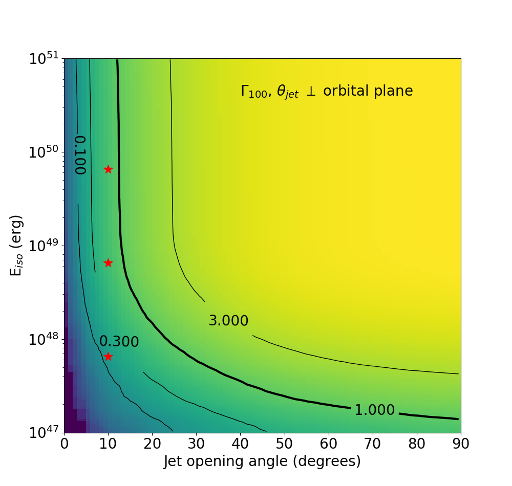
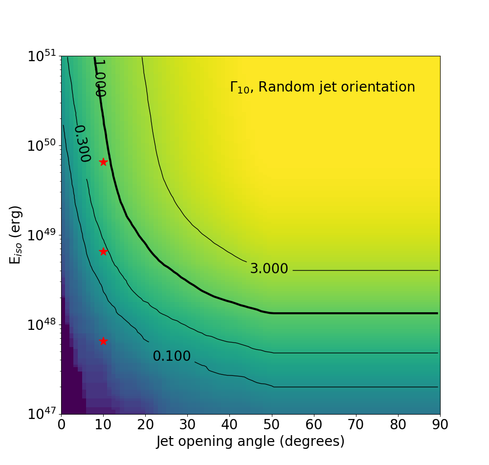
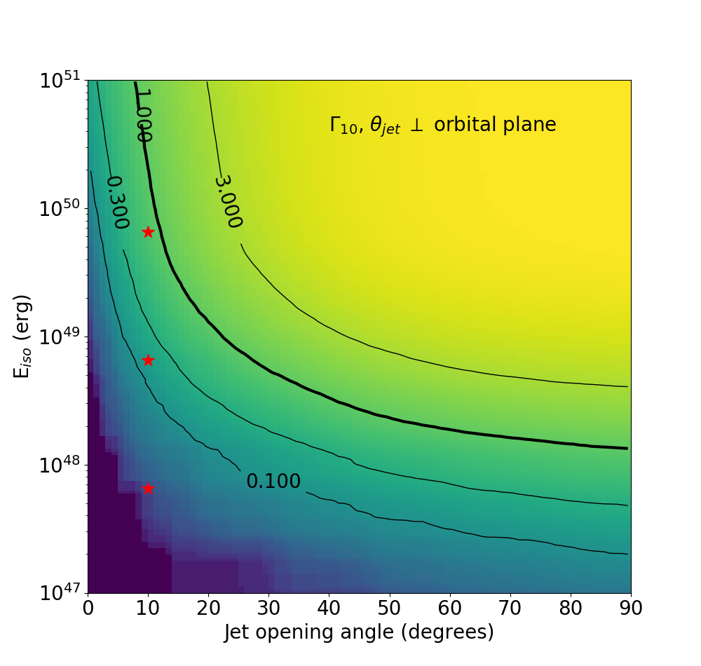
Figure 8: Average number of events with $\gamma$-ray flux above the Fermi/GBM threshold, out of 10 GW-detected BBH mergers. The stars indicate the models studied in more detail here. By allowing at most one $\gamma$-ray detection in the sample, the permitted parameter space is restricted to the range $[(E_{\rm iso}/10^{48}{\rm erg})(\theta_{\rm jet}/20^{\circ})-(E_{\rm iso}/10^{49}{\rm erg})(\theta_{\rm jet}/20^{\circ})]\lesssim 1$, with the specific value dependent on the Lorentz factor and on the relative inclination of the jet with respect to the orbital plane of the merging BBHs.

5 Constraints on emission models from EM follow-ups to LIGO BBHs mergers to date

LIGO and Virgo have detected 10 BH-BH mergers during the first two observing runs O1 and O2 (The LIGO Scientific Collaboration & the Virgo Collaboration, 2018). Among all the models studied here, the probability of detecting EM emission in $\gamma$-rays above the Fermi/GBM threshold is the largest ($\sim 5-7$%) for $\theta_{\rm jet}\perp$ orbital plane, and the highest energy case ($E_{48}$), as well as for $E_{47}\Gamma_{100}$. Thus, for 10 events with energetics and $\Gamma$ factors in that range, we would expect to see an average of $\sim 0.5$ event. Therefore the tentative detection of one counterpart in $\gamma$-rays would not be surprising. As a reference, recall that the inferred isotropic energy of that event is $10^{49}$ ergs, which translates into a jet energy of $10^{49}(1-\cos\theta_{\rm jet})$. For $\theta_{\rm jet}=10^{\circ}$, this is $1.5\times 10^{47}$ erg.

We further generalize the above constraint by running an extended series of Monte Carlo simulations for a wider range of jet angles and isotropic equivalent energies; for each combination, we compute the average number of events (out of 10 GW-detected BBH mergers) with $\gamma$-ray flux above the Fermi/GBM detection threshold. The results are reported in Fig.8, for both the low and high $\Gamma$ models, as well as the two scenarios for the direction of $\theta_{\rm jet}$. The stars indicate the three $[E_{\rm iso}\theta_{\rm jet}]$ combinations studied in more detail here. As expected, larger energetics require smaller jet angles in order not to overpredict the number of events with a $\gamma$-ray detection. Allowing the number of detections to be no more than 1 out of 10, we can already restrict the permitted parameter space to the range $[(E_{\rm iso}/10^{48}{\rm erg})(\theta_{\rm jet}/20^{\circ})-(E_{\rm iso}/10^{49}{\rm erg})(\theta_{\rm jet}/20^{\circ})]\lesssim 1$, with the specific value dependent on the Lorentz factor and on the relative inclination of the jet with respect to the orbital plane of the merging BBHs.

At longer wavelengths, there have been no reported EM counterparts from follow ups to the first 6 BBH merger events. Assuming that the situation remains the same after the complete follow up catalogue has been published, the probability of one detection in the best case scenario and with continuous follow up is at most $\sim 30\%$. Therefore, the current (afterglow) data set cannot be used as yet to rule out jet production within the range of models studied here. However, we remind once again that our afterglow models have been run for a fixed density value ($n=0.01$ cm^-3). Merger events in denser regions would have brighter emission than the one computed here, and hence detection probabilities have a degree of degeneracy between the source properties and the ambient ones. To allow the community to use our results to restrict the allowed parameter space by means of each new followup in some energy band and at some specific observing time, we have put our current models online, and we are populating them further with models run with a wider range of parameters.

6 Summary and Discussion

The detection of GWs from binary black hole mergers has provided yet another confirmation of the theory of General Relativity. However, the tentative detection of an EM counterpart to GW150917 (Connaughton et al., 2016) had not been predicted by any theory, and hence it gave rise to a number of ideas of different nature, from the mundane to the exotic. If EM radiation from merging BHs was detected at high confidence, it would thus revolutionize our pre-concepts of merging BHs.

While the energy production mechanisms proposed for EM emission are diverse, a common feature to a sudden release of energy is the formation of a relativistic shock which plows into the medium, giving rise to radiation spanning a wide electromagnetic range, from $\gamma$-rays to radio. Both simulations and observations of this phenomenon have shown that the radiating outflow is jetted. Emission at wide angles is dominated by interaction of the jet with surrounding dense material, as demonstrated by the binary NS merger GW170917; in this case the interacting material is provided by the tidally disrupted matter of the neutron stars. Such ejecta is however not present in the case of a BBH merger, resulting in much weaker angular emission.

Assessing the detection probability of EM emission is of paramount importance in order to be able to extract meaningful information as more data are gathered from EM followups to BBH mergers. To this aim, here we have performed a Monte Carlo simulation of a population of BBH mergers, with a redshift distribution derived from the current observed population, and for a range of energies and Lorentz factors of possible jets driven at the time of the merger. The angular emission of the jet in different energy bands has been numerically calculated for each event as a function of time.

Among the models which we explored in detail, we find that, in $\gamma$-rays, the detection probability with the Swift/XRT and Fermi/GBM bands is up to $\sim$6-7% in the model with the largest jet energy, $E_{48}$, and with the direction of the jet aligned with the orbital angular momentum of the merging BHs (since these events are more easily detectable by LIGO). The probability for detection in $\gamma$ is largely determined by the angular size of the jet, since at early times the high Doppler factor largely suppresses the side emission. Hence, to generalize and further explore the consequences of our results for $\gamma$-ray followups to date, we additionally ran a grid of models for a much larger range of jet energies and jet opening angles. The condition that $\lesssim 1$ event out of 10 GW-detected BBH mergers is above the Fermi/GBM threshold imposes that any currently allowed emission model has to satisfy the condition $(E_{\rm iso}/10^{49}{\rm erg})(\theta_{\rm jet}/20^{\circ})\lesssim 1$ for the most favorable scenario.

At longer wavelengths, the detection probability in each band becomes time-dependent, and the precise time of the maximum depends on a combination of the fireball parameters, such as its energy and initial Lorentz factor, and the viewing angle to the observer. However, even in the best case model studied here, the detection probability with current observational facilities in typical observation bands (X, O, R) is at most around 3%. Early followups, within a day, yield higher chances of catching the afterglow radiation.

Lack of detection of X-ray through radio emission from the first 10 LIGO/Virgo events (assuming that the complete catalogue has the same properties of the first 6 events) remains still unconstraining for the range of models studied here, since the detection probability would be at most $\sim 30\%$. More events are needed before being able to put more stringent constraints down to the energy levels considered here (unless jets were considerably wider than $\sim 10^{\circ}$ and/or the ambient density of the medium in which the merger occurred was on average much larger than $\sim 0.01$ cm^-3).

Finally, note that the EM detection probabilities that we have calculated here have assumed the detection sensitivity of LIGO/Virgo in runs O1/O2. As the sensitivity to GW detection improves in future runs, the probability of observing EM radiation in followups to GW-detected BBH mergers decreases, since more events will be detected from higher redshifts, and hence they will appear on average dimmer to the observer (for the same model parameters). The total number of GW events (and hence potential follow ups) will however increase, and hence it will be important to have a wide range of models to compare against. While here we have reported and discussed the results of a few representative cases, we are building a public, online library of models in several representative bands for a much wider range of parameters. Our library (see footnote 6 for location) will allow to use each new limit on EM emission to carve out a region of highly disfavored emission models, so that, over the years to come, we will learn how dark BBHs mergers actually are. Future missions with higher sensitivity than the current facilities, such as the James Webb Space Telescope, will play a crucial role in this pursuit.

References

- Abbott et al. (2016a) Abbott, B. P., Abbott, R., Abbott, T. D., et al. 2016a, Physical Review Letters, 116, 061102, doi: 10.1103/PhysRevLett.116.061102
- Abbott et al. (2016b) —. 2016b, Physical Review X, 6, 041015, doi: 10.1103/PhysRevX.6.041015
- Abbott et al. (2016c) —. 2016c, ApJ, 833, L1, doi: 10.3847/2041-8205/833/1/L1
- Abbott et al. (2016d) —. 2016d, Physical Review Letters, 116, 241103, doi: 10.1103/PhysRevLett.116.241103
- Abbott et al. (2016e) —. 2016e, ApJ, 826, L13, doi: 10.3847/2041-8205/826/1/L13
- Abbott et al. (2016f) —. 2016f, The Astrophysical Journal Supplement Series, 227, 14, doi: 10.3847/0067-0049/227/2/14
- Abbott et al. (2017a) —. 2017a, ApJ, 848, L13, doi: 10.3847/2041-8213/aa920c
- Abbott et al. (2017b) —. 2017b, Physical Review Letters, 118, 221101, doi: 10.1103/PhysRevLett.118.221101
- Abbott et al. (2017c) —. 2017c, ApJ, 851, L35, doi: 10.3847/2041-8213/aa9f0c
- Abbott et al. (2018) —. 2018, Living Reviews in Relativity, 21, 3, doi: 10.1007/s41114-018-0012-9
- Aloy et al. (2005) Aloy, M. A., Janka, H.-T., & Müller, E. 2005, A&A, 436, 273, doi: 10.1051/0004-6361:20041865
- Band (1997) Band, D. L. 1997, ApJ, 486, 928, doi: 10.1086/304566
- Bartos et al. (2017) Bartos, I., Kocsis, B., Haiman, Z., & Márka, S. 2017, ApJ, 835, 165, doi: 10.3847/1538-4357/835/2/165
- Bhat et al. (2016) Bhat, P. N., Meegan, C. A., von Kienlin, A., et al. 2016, VizieR Online Data Catalog, 222
- Blandford & Znajek (1977) Blandford, R. D., & Znajek, R. L. 1977, MNRAS, 179, 433, doi: 10.1093/mnras/179.3.433
- Connaughton et al. (2016) Connaughton, V., Burns, E., Goldstein, A., et al. 2016, ApJ, 826, L6, doi: 10.3847/2041-8205/826/1/L6
- de Mink & King (2017) de Mink, S. E., & King, A. 2017, ApJ, 839, L7, doi: 10.3847/2041-8213/aa67f3
- Eichler & Waxman (2005) Eichler, D., & Waxman, E. 2005, ApJ, 627, 861, doi: 10.1086/430596
- Fishbach et al. (2018) Fishbach, M., Holz, D. E., & Farr, W. M. 2018, ApJ, 863, L41, doi: 10.3847/2041-8213/aad800
- Fong et al. (2015) Fong, W., Berger, E., Margutti, R., & Zauderer, B. A. 2015, ApJ, 815, 102, doi: 10.1088/0004-637X/815/2/102
- Fraschetti (2018) Fraschetti, F. 2018, JCAP, 4, 054, doi: 10.1088/1475-7516/2018/04/054
- Gruber et al. (2014) Gruber, D., Goldstein, A., Weller von Ahlefeld, V., et al. 2014, The Astrophysical Journal Supplement Series, 211, 12, doi: 10.1088/0067-0049/211/1/12
- Hogg (1999) Hogg, D. W. 1999, ArXiv Astrophysics e-prints
- Janiuk et al. (2017) Janiuk, A., Bejger, M., Charzyński, S., & Sukova, P. 2017, New A, 51, 7, doi: 10.1016/j.newast.2016.08.002
- Kathirgamaraju et al. (2019) Kathirgamaraju, A., Tchekhovskoy, A., Giannios, D., & Barniol Duran, R. 2019, MNRAS, 484, L98, doi: 10.1093/mnrasl/slz012
- Khan et al. (2018) Khan, A., Paschalidis, V., Ruiz, M., & Shapiro, S. L. 2018, Phys. Rev. D, 97, 044036, doi: 10.1103/PhysRevD.97.044036
- Lazzati et al. (2017a) Lazzati, D., Deich, A., Morsony, B. J., & Workman, J. C. 2017a, MNRAS, 471, 1652, doi: 10.1093/mnras/stx1683
- Lazzati et al. (2017b) Lazzati, D., López-Cámara, D., Cantiello, M., et al. 2017b, ApJ, 848, L6, doi: 10.3847/2041-8213/aa8f3d
- Lazzati et al. (2018) Lazzati, D., Perna, R., Morsony, B. J., et al. 2018, Physical Review Letters, 120, 241103, doi: 10.1103/PhysRevLett.120.241103
- Liebling & Palenzuela (2016) Liebling, S. L., & Palenzuela, C. 2016, Phys. Rev. D, 94, 064046, doi: 10.1103/PhysRevD.94.064046
- Liu et al. (2016) Liu, T., Romero, G. E., Liu, M.-L., & Li, A. 2016, ApJ, 826, 82, doi: 10.3847/0004-637X/826/1/82
- Loeb (2016) Loeb, A. 2016, ApJ, 819, L21, doi: 10.3847/2041-8205/819/2/L21
- Martin et al. (2018) Martin, R. G., Nixon, C., Xie, F.-G., & King, A. 2018, MNRAS, 480, 4732, doi: 10.1093/mnras/sty2178
- Medvedev & Loeb (1999) Medvedev, M. V., & Loeb, A. 1999, ApJ, 526, 697, doi: 10.1086/308038
- Murase et al. (2016) Murase, K., Kashiyama, K., Mészáros, P., Shoemaker, I., & Senno, N. 2016, ApJ, 822, L9, doi: 10.3847/2041-8205/822/1/L9
- Nishikawa et al. (2009) Nishikawa, K.-I., Niemiec, J., Hardee, P. E., et al. 2009, ApJ, 698, L10, doi: 10.1088/0004-637X/698/1/L10
- Panaitescu & Kumar (2001) Panaitescu, A., & Kumar, P. 2001, ApJ, 560, L49, doi: 10.1086/324061
- Perna et al. (2018) Perna, R., Chruslinska, M., Corsi, A., & Belczynski, K. 2018, MNRAS, 477, 4228, doi: 10.1093/mnras/sty814
- Perna et al. (2016) Perna, R., Lazzati, D., & Giacomazzo, B. 2016, ApJ, 821, L18, doi: 10.3847/2041-8205/821/1/L18
- Sari et al. (1998) Sari, R., Piran, T., & Narayan, R. 1998, ApJ, 497, L17, doi: 10.1086/311269
- The LIGO Scientific Collaboration & the Virgo Collaboration (2018) The LIGO Scientific Collaboration, & the Virgo Collaboration. 2018, ArXiv e-prints, arXiv:1811.12907. https://arxiv.org/abs/1811.12907
- The LIGO Scientific Collaboration et al. (2018) The LIGO Scientific Collaboration, the Virgo Collaboration, Abbott, B. P., et al. 2018, arXiv e-prints, arXiv:1811.12940. https://arxiv.org/abs/1811.12940
- Wang et al. (2015) Wang, X.-G., Zhang, B., Liang, E.-W., et al. 2015, ApJS, 219, 9, doi: 10.1088/0067-0049/219/1/9
- Woosley (2016) Woosley, S. E. 2016, ApJ, 824, L10, doi: 10.3847/2041-8205/824/1/L10
- Yamazaki et al. (2016) Yamazaki, R., Asano, K., & Ohira, Y. 2016, Progress of Theoretical and Experimental Physics, 2016, 051E01, doi: 10.1093/ptep/ptw042
- Zhang (2016) Zhang, B. 2016, ApJ, 827, L31, doi: 10.3847/2041-8205/827/2/L31