Decentralized Poisson Multi-Bernoulli Filtering for Vehicle Tracking

Abstract

A decentralized Poisson multi-Bernoulli filter is proposed to track multiple vehicles using multiple high-resolution sensors. Independent filters estimate the vehicles’ presence, state, and shape using a Gaussian process extent model; a decentralized filter is realized through fusion of the filters posterior densities. An efficient implementation is achieved by parametric state representation, utilization of single hypothesis tracks, and fusion of vehicle information based on a fusion mapping. Numerical results demonstrate the performance.

I Introduction

Multitarget tracking (MTT), i.e., tracking of independently moving targets, is important for surveillance and safety applications [1, 2]. Traditionally, it has been developed for surveillance of the sky using ground-to-air radar sensors. An multitarget tracking (MTT) filter allows to incorporate the peculiarities of those kind of sensors: false alarm measurements due to clutter; missed detections; unknown measurement-to-target correspondence; and target appearance and disappearance; which are all challenges that arise for radar-like sensors. In many typical MTT scenarios, the sensor resolution is low with respect to (w.r.t.) the target size, and a reasonable assumption is to model the targets as points having a kinematic state (e.g., position and velocity). An elegant way to track multiple targets is via the Poisson multi-Bernoulli mixture (PMBM) filter [3, 4], which preserves a PMBM form during prediction and update steps.

With the availability of high resolution sensors, the point target assumption does not hold anymore, see, e.g., [5]. For instance, a high resolution Lidar sensor can obtain in one scan multiple detections from a single vehicle [6] or cyclist [7]. This is because the sensor resolution is high w.r.t. the target (here, a vehicle) size. In such an application scenario, the vehicle extent needs to be modeled (and estimated) as well in the MTT filter, leading to an ETT filter. In ETT, extended targets give rise to possibly multiple noisy detections, the vehicle extent (shape and size) is a priori unknown and may vary over time, and the objective is to estimate the ET’s kinematic state as well as its extent [5]. A common model for the ET extent is based on Gaussian process (GP) modelling [8, 9].

Neither MTT nor ETT filters are bound to single sensors. When multiple sensors are used, it becomes necessary to fuse the information from the different sensors. Centralized fusion consists of transmitting all measurements to a central processing unit. Decentralized fusion consists of local processing (i.e., perform recursive state-space estimation) at each sensor unit, and transmission of the tracking results. Such an approach was proposed in [10], for fusing two multi-Bernoulli (MB) densities, though it did not account for a Poisson point process (PPP) component.

In this paper, we utilize and extend the shape model from [8, 9], and integrate it into an ETT filter, which allows tracking of multiple ETs. The resulting ETT filter’s multiobject posterior is of the so-called PMB form [11]. Furthermore, we propose a novel fusion strategy that performs fusion separately for the PPP and MB parts of the PMB density. The implementation of the PMB filter yields a tracking filter with low computational cost locally at each sensor, and globally low computational cost through the introduction of a fusion map based on the Kullback-Leibler divergence (KLD) between target tracks. Simulation results demonstrate the performance of the proposed independent ETT filter as well as of the decentralized ETT filtering approach. The main contributions of this paper are:

• We apply a state-of-the-art ETT filter [3, 4] and propose a novel distributed fusion strategy based on the Kullback-Leibler average (KLA) by fusion of the filters’ posterior multiobject densities of PMB form; and

• We enable low complexity in distributed fusion through introduction of a fusion map based on KLD between target tracks.

• We extend, in Section VII-A2, the GP model from [8, 9] for the ET shape description to a multisensor scenario incorporating the sensors’ state (position, orientation);

The remainder of this paper is organized as follows; Section II presents relevant related work to this paper’s work, Section III gives some background knowledge on random finite sets, and Section IV introduces the system model and the problem formulation. Section V details the proposed ETT filter, Section VI presents the decentralized posterior fusion approach using independent ETT filters. Simulation results are given in Section VII, and conclusions are drawn in Section VIII.

II Related work

Here, we discuss related work relevant for this paper’s work covering extent modeling for tracking an ET, ETT, and information fusion with multiple sensors.

II-A Extent modelling

Different models for the target extent (shape and size) exist in ETT, which may be classed according to complexity, ranging from assuming a specific geometric shape [12, 7, 6] with, e.g., unknown translation and rotation, to models that describe general shapes, see, e.g., [13, 14, 15]. Typically, more complex models provide a richer shape description. Two popular models are the random matrix approach [12], where the target shape is described by an ellipsoid; and a GP based approach [8, 9], where a star convex target shape is described by a GP. See [5] for an extensive overview of works on ETT.

II-B Tracking multiple extended targets

For tracking multiple extended targets, several different filters have been developed: PHD filter [16, 17, 18, 19]; Cardinalized (CPHD) filter [20]; $\delta$-generalized labelled multi-Bernoulli ($\delta$-GLMB) filter [21]; and PMBM filter [3, 4]. Multiple extended target tracking filters have been applied to tracking of different target types (e.g., for cars [22, 23, 24]).

The $\delta$-GLMB filter and PMBM filter are so called multi-object conjugate priors, meaning that if we start with the conjugate density form ($\delta$-GLMB or PMBM), then all subsequent predicted and updated densities will be of the same form. Based on the conjugate priors, computationally cheaper, approximate filters have been presented. The labeled multi-Bernoulli (LMB) filter is an approximation of the $\delta$-GLMB filter, see [21]. The PMB filter is an approximation of the PMBM filter, see [11, 25].

The PMBM conjugate prior [26] was originally developed for point targets; a PMBM conjugate prior for extended targets was presented in [4, 3]. In several simulation studies it has been shown that, compared to tracking filters built upon labelled RFS, the PMBM conjugate prior has good performance for tracking the set of present target states, for both point targets [27, 28, 29] and extended targets [4, 3, 30].

The PMBM conjugate priors for point targets and extended targets have been shown to be versatile, and have been used with data from Lidars [31, 32, 33, 34], radars [32, 33], and cameras [35, 33]. They have been successfully applied not only to tracking of moving targets, but also mapping of stationary objects [36], as well as joint tracking and sensor localisation [37]. Thus, it is well motivated to use the PMBM filter in this work; specifically, we work with the computationally cheaper PMB filter. Developing similar decentralized tracking algorithms for the $\delta$-GLMB or LMB filter [21] is a topic for future work.

II-C Tracking using multiple sensors

Different approaches to incorporate measurements from multiple sensors which were acquired within one scan exist, where the simplest may be seen as performing multiple update steps (e.g., Kalman update or likewise) by augmenting the measurement model to incorporate all sensor models, see, e.g., [38].

When sensors are geographically separated, measurements from all sensors need to be transmitted to the central processing unit where the filter is run. In the absence of such a central unit or simply due to the limited capacity of the communication channel, one can perform filtering already at the sensor and share only target track information, e.g., the parameters of a known probability density function (PDF) family. Through incorporation of target track information obtained by independent filters, a decentralized filtering approach (i.e., information fusion) can be realized without the need for additional prior information. Such methods need to ensure that (unknown) common information obtained by the independent tracking filters is not double counted, e.g., the prior target density [39].

Depending on the type of posterior multiobject density in MTT/ETT filtering, several sub-optimal information fusion strategies have been developed based on, e.g, covariance intersection (CI) for Gaussian densities. This replaces the product form of Bayes’ rule with the KLA. CI (and consequently KLA) is a method to fuse information with unknown priors in a robust way in the sense that the fused posterior is conservative and never overconfident about the estimates and thus implicitly sub-optimal [39, 40]. Examples of CI/KLA include fusion of Bernoulli and independent identically distributed (IID) cluster processes posteriors [41], fusion for Bernoulli filters [42], fusion for PHD and CPHD filters [43, 44, 45, 46, 47, 48], and fusion for LMB filters [47, 10, 49].

III Background on Random Finite Sets

Two types of RFSs relevant for this work deserve special attention: Bernoulli RFS, and a PPP. They can be extended to MB RFS, multi-Bernoulli mixture (MBM) RFS and combined in a PMBM RFS. These are described below, for more details on RFSs the reader is referred to [50].

III-A Common RFS densities

Bernoulli RFS

A Bernoulli RFS $\boldsymbol{X}$ has a multiobject density [50]

$$f(\boldsymbol{X})=\begin{cases}1-r,&\boldsymbol{X}=\emptyset,\\ rf(\boldsymbol{x}),&\boldsymbol{X}=\{\boldsymbol{x}\},\\ 0,&|\boldsymbol{X}|\geq 2,\end{cases}$$ (1)

where $r\in[0,1]$ denotes the probability that a target exists and if it exists $f(\boldsymbol{x})$ is its PDF.

Multi-Bernoulli RFS

An MB RFS is the disjoint union of independent Bernoulli RFSs indexed by $i$. It is fully parametrized by $\{r_{i},f_{i}(\boldsymbol{x})\}_{i\in\mathbb{I}}$, where $\mathbb{I}$ is its index set. For $\boldsymbol{X}=\{\boldsymbol{x}_{1},\ldots,\boldsymbol{x}_{n}\}$, the multiobject density can be written as

$$f(\boldsymbol{X})=\sum_{\uplus_{i\in\mathbb{I}}\boldsymbol{X}_{i}=\boldsymbol{X}}\prod_{i\in\mathbb{I}}f_{i}(\boldsymbol{X}_{i})$$ (2)

for $|\boldsymbol{X}|\leq|\mathbb{I}|$, and $f(\boldsymbol{X})=0$ otherwise. The notation, $\boldsymbol{X}_{1}\uplus\boldsymbol{X}_{2}=\boldsymbol{X}$ means $\boldsymbol{X}_{1}\cup\boldsymbol{X}_{2}=\boldsymbol{X}$ and $\boldsymbol{X}_{1}\cap\boldsymbol{X}_{2}=\emptyset$.

Multi-Bernoulli Mixture RFS

The multiobject density of an MBM is the normalized, weighted sum of multiobject densities of MBs, which can be stated as [3]

$$f(\boldsymbol{X})=\sum_{j\in\mathbb{J}}w_{j}\sum_{\uplus_{i\in\mathbb{I}^{j}}\boldsymbol{X}_{i}=\boldsymbol{X}}\prod_{i\in\mathbb{I}^{j}}f_{j,i}(\boldsymbol{X}_{i}).$$ (3)

The MBM multiobject density is parametrized by $\{w_{j,i},\{r_{j,i},f_{j,i}(\boldsymbol{x})\}_{i\in\mathbb{I}^{j}}\}_{j\in\mathbb{J}}$, where $w_{j}$ is the weight of MB $j$, and $\mathbb{J}$ is the index set of the MBs in the MBM. An MB is therefore a special case of an MBM with $|\mathbb{J}|=1$.

PPP

A PPP is a type of RFS, where the cardinality follows a Poisson distribution, and its elements are IID. It is parametrized by the intensity function $D(\boldsymbol{x})=\lambda f(\boldsymbol{x})$, where $\lambda>0$ is the Poisson rate and $f(\boldsymbol{x})$ is a PDF on the single element state $\boldsymbol{x}$. The multiobject density of a PPP is [50, 3]

$$f(\boldsymbol{X})=e^{-\lambda}\prod_{i=1}^{n}\lambda f(\boldsymbol{x}_{i}).$$ (4)

PMBM

An PMBM RFS is the disjoint set union of an PPP and an MBM having multiobject density [3]

$$f(\boldsymbol{X})=\sum_{\boldsymbol{X}^{u}\uplus\boldsymbol{X}^{d}=\boldsymbol{X}}f^{u}(\boldsymbol{X}^{u})f^{d}(\boldsymbol{X}^{d}),$$ (5)

where $f^{u}(\cdot)$ has multiobject density (4), and $f^{d}(\boldsymbol{X}^{d})$ has multiobject density (3). For $|\mathbb{J}|=1$, (5) is called a PMB distribution.

III-B RFS Bayesian Filter

Similar to the random vector (RV) case, an RFS based filter can be described, conceptually at least, within the Bayesian filtering framework by performing a prediction step using the motion model [2, Ch. 14]

$$f_{+}(\boldsymbol{X}) =\int f(\boldsymbol{X}|\boldsymbol{X}^{\prime})f_{-}(\boldsymbol{X}^{\prime})\delta\boldsymbol{X}^{\prime},$$ (6)

where $f_{-}(\boldsymbol{X}^{\prime})$ is the prior RFS density, $f(\boldsymbol{X}|\boldsymbol{X}^{\prime})$ is the multiobject process model, and a Bayesian update step

$$f(\boldsymbol{X}|\boldsymbol{Z})\propto\ell(\boldsymbol{Z}|\boldsymbol{X})f_{+}(\boldsymbol{X}).$$ (7)

Here, $f_{+}(\boldsymbol{X})$ is the predicted RFS density, and $\ell(\boldsymbol{Z}|\boldsymbol{X})$ is the RFS measurement likelihood for measurement set $\boldsymbol{Z}$.

A typical way to estimate the set states from a Bernoulli process with RFS density $f(\boldsymbol{X})$ is by comparing the probability of existence $r$ to an existence threshold $r_{\mathrm{th}}$. For $r>r_{\mathrm{th}},$ the target is said to exist and has PDF $f(\boldsymbol{x})$. Its state can then be estimated by the mean $\hat{\boldsymbol{x}}=\int\boldsymbol{x}f(\boldsymbol{x})\mathrm{d}\boldsymbol{x}$. See, e.g., [28] for a elongated discussion on multiobject estimation.

IV Problem Formulation and System Model

Here, we present first the problem formulation of this paper followed by the ET state and transition model and the ET set measurement likelihood function.

IV-A Problem Formulation

We consider a scenario with ${N}_{\mathrm{sens}}$ sensing systems (each composed of sensors plus filter), each collecting measurements using its local sensors, with the aim to jointly surveil an environment $\mathcal{E}$ where vehicles pass (c.f. Fig. 1). Our goals are (i) to derive a low-complexity PMB-ETT filter for each sensing system $s=1,2,\ldots,{N}_{\mathrm{sens}}$, computing in every time step $k$ the posterior density $f_{s}(\boldsymbol{X}_{k}|\boldsymbol{Z}_{s,k:1})$ of the ETs, using only its own sensors with measurement set $\boldsymbol{Z}_{s,k:1}$; and (ii) to derive a decentralized method to combine posterior information of ETs obtained by ${N}_{\mathrm{sens}}$ independent ETT filters in order to obtain a global posterior density $\bar{f}_{w}(\boldsymbol{X}_{k}|\boldsymbol{Z}_{1,k:1},\boldsymbol{Z}_{2,k:1},\ldots,\boldsymbol{Z}_{{N}_{\mathrm{sens}},k:1})$ (i.e., using only the posterior densities of each ETT filter).

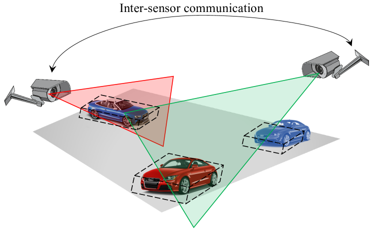
Figure 1: Scenario with three ETs observed by two sensors with partially overlapping FoVs.

IV-B ET State and Transition Model

A standard motion model for the ET is assumed, where ET motion follows IID Markov processes with single ET transition PDF $f_{k+1|k}(\boldsymbol{x}_{k+1}|\boldsymbol{x}_{k})$, where $\boldsymbol{x}_{k}$ denotes the state at time $k$. Targets arrive according to a non-homogeneous PPP with intensity $D^{b}(\boldsymbol{x}_{k})$, and depart according to IID Markov processes, where the survival probability in $\boldsymbol{x}_{k}$ is $p_{\mathrm{S}}(\boldsymbol{x}_{k})$. Additionally to this, $\boldsymbol{x}_{k}$ comprises an unknown Poisson rate $\gamma_{k}$ describing the average number of measurements generated by the ET and the ET spatial state ${\boldsymbol{y}}_{k}$ (this will become clear in Sec. VII-A where a detailed description of the state and transition density is provided).

IV-C ET Set Measurement Likelihood Function

In one scan, a sensor receives a set of measurements $\boldsymbol{Z}$ consisting of target-generated measurements $\boldsymbol{z}$ and clutter, where the ETs are independently detected with state-dependent probability of detection $p_{\mathrm{D}}(\boldsymbol{x})$, which depends on the sensor FoV. Clutter is modeled by a PPP with intensity $\kappa(\boldsymbol{z})=\lambda c(\boldsymbol{z})$ with mean $\lambda$ and spatial distribution $c(\boldsymbol{z})$. Target-generated measurements are modeled by a PPP with intensity $\gamma(\boldsymbol{x})f(\boldsymbol{z}|\boldsymbol{x})$, where both the Poisson measurement rate $\gamma(\boldsymbol{x})$ and the single measurement likelihood $f(\boldsymbol{z}|\boldsymbol{x})$ are state dependent. The measurement likelihood for ETs $\{\boldsymbol{x}_{1},\ldots,\boldsymbol{x}_{n}\}$ and measurement set $\boldsymbol{Z}$ is

$$\ell(\boldsymbol{Z}|\{\boldsymbol{x}_{1},\ldots,\boldsymbol{x}_{n}\})=$$

$$e^{-\lambda}\sum_{\boldsymbol{Z}_{c}\uplus\boldsymbol{Z}_{1}\uplus\ldots\boldsymbol{Z}_{n}=\boldsymbol{Z}}[c(\cdot)]^{\boldsymbol{Z}_{c}}\prod_{i=1}^{n}\ell_{\boldsymbol{Z}_{i}}(\boldsymbol{x}_{i}),$$ (8)

where $[c(\cdot)]^{\boldsymbol{Z}_{c}}$ is shorthand for $\prod_{\boldsymbol{z}\in\boldsymbol{Z}_{c}}c(\boldsymbol{z})$, $[c(\cdot)]^{\emptyset}=1$ by definition, and [3]

$$\ell_{\boldsymbol{Z}}(\boldsymbol{x})=\begin{cases}p_{\mathrm{D}}(\boldsymbol{x})e^{-\gamma(\boldsymbol{x})}\prod_{\boldsymbol{z}\in\boldsymbol{Z}}\gamma(\boldsymbol{x})f(\boldsymbol{z}|\boldsymbol{x}),&|\boldsymbol{Z}|>0,\\ (1-p_{\mathrm{D}}(\boldsymbol{x}))+p_{\mathrm{D}}(\boldsymbol{x})e^{-\gamma(\boldsymbol{x})},&\boldsymbol{Z}=\emptyset.\end{cases}$$ (9)

Note that (i) equation (8) involves potentially multiple ETs, leading to a data association (DA) problem; (ii) a single ET can generate multiple measurements.

V Independent PMB-ETT Filter

In this section, we briefly describe the processing performed by each - (PMB-ETT) filter from [3]. We omit the time index $k$ for brevity. The PMB model is a combination of a PPP describing the distribution of unknown targets, i.e., targets which are hypothesized to exist, but have not yet been detected; and a MB which describes targets that have been detected at least once. The target set can therefore be split into two disjoint subsets $\boldsymbol{X}=\boldsymbol{X}^{u}\uplus\boldsymbol{X}^{d}$ corresponding to the unknown target set $\boldsymbol{X}^{u}$ (with PPP intensity $D^{u}(\boldsymbol{x})$, modelled as a non-normalized mixture density with mixture components located in the region of interest, denoted $\mathcal{E}$) and the detected target set $\boldsymbol{X}^{d}$ with density $f^{d}(\boldsymbol{X}^{d})$ and index set $\mathbb{I}$. Hence, the PMB density is fully described by a MB component described by $\{r^{i},f^{i}(\boldsymbol{x})\}_{i\in\mathbb{I}}$ and a PPP component $D^{u}(\boldsymbol{x})$.

V-1 PMB-ETT Filter Prediction

The predicted density is a PMB density with parameters [3, Sec. IV], [4]

$$D_{+}^{u}= D^{b}(\boldsymbol{x})+\left\langle D^{u},p_{\mathrm{S}}f_{k+1|k}\right\rangle,$$ (10)

$$r_{+}^{i}= \left\langle f^{i},p_{\mathrm{S}}\right\rangle r^{i},$$ (11)

$$f_{+}^{i}= \frac{\left\langle f^{i},p_{\mathrm{S}}f_{k+1|k}\right\rangle}{\left\langle f^{i},p_{\mathrm{S}}\right\rangle},$$ (12)

where $\left\langle g,h\right\rangle=\int g(\boldsymbol{x})f(\boldsymbol{x})\mathrm{d}\boldsymbol{x}$ denotes the inner product. The proof of the prediction step can be found in, e.g., [11].

V-2 PMB-ETT Filter Update

We introduce the set of valid DAs $\mathcal{A}=\mathcal{P}(\mathbb{M}\cup\mathbb{I})$, where $\mathbb{M}$ is the index set for $\boldsymbol{Z}$. Here, $A\in\mathcal{A}$ is a partition of $\mathbb{M}\cup\mathbb{I}$ into non-empty disjoint subsets $C\in A$ (called index cells), with the constraint that for each $C:|C\cap\mathbb{I}|\leq 1$ (i.e., measurements can only be associated with a single target). When $|C\cap\mathbb{I}|=1$, let the entry in $C\cap\mathbb{I}$ be denoted by $i_{C}$ and let $\boldsymbol{C}_{C}=\cup_{m\in C\cap\mathbb{M}}\boldsymbol{z}_{m}$ contain the associated measurements. Given the predicted prior PMB density with parameters (10), (11), (12), and a set of measurements $\boldsymbol{Z}$; the updated density is a PMBM density [3, Sec. IV], [4]

$$f(\boldsymbol{X}|\boldsymbol{Z})= \sum_{\boldsymbol{X}^{u}\uplus\boldsymbol{X}^{d}=\boldsymbol{X}}f^{u}(\boldsymbol{X}^{u})\sum_{A\in\mathcal{A}}w_{A}f_{A}^{d}(\boldsymbol{X}^{d}),$$ (13)

$$f^{u}(\boldsymbol{X}^{u})= e^{-\left\langle D^{u},1\right\rangle}\prod_{\boldsymbol{x}\in\boldsymbol{X}^{u}}D^{u}(\boldsymbol{x}),$$ (14)

$$f_{A}^{d}(\boldsymbol{X}^{d})= \sum_{\uplus_{C\in A}\boldsymbol{X}^{C}=\boldsymbol{X}^{d}}\prod_{C\in A}f_{C}(\boldsymbol{X}^{C}),$$ (15)

$$D^{u}(\boldsymbol{x})= q_{\mathrm{D}}(\boldsymbol{x})D_{+}^{u}(\boldsymbol{x}),$$ (16)

where $f_{C}(\boldsymbol{X}^{C})$ is a Bernoulli density, with existence probability and spatial distribution provided in Appendix A, together with the weights $w_{A}$ of each DA hypothesis. Above, $q_{\mathrm{D}}(\boldsymbol{x})$ denotes the probability that the target $\boldsymbol{x}$ is not detected and is defined as

$$q_{\mathrm{D}}(\boldsymbol{x})=1-p_{\mathrm{D}}(\boldsymbol{x})+p_{\mathrm{D}}(\boldsymbol{x})e^{-\gamma(\boldsymbol{x})}.$$ (17)

To reduce computational complexity, we use standard methods and truncate the space of possible partitions by clustering measurements and consider DA w.r.t. different clusters [17, 18, 20]. Finally, the PMBM in (13) is converted to a PMB, which was detailed in [51] for point targets and in [25] for ETs.

VI Decentralized Posterior Fusion

Here, we present the decentralized approach to robust fusion of posterior densities $f_{s}(\boldsymbol{X}|\boldsymbol{Z}_{s})$ computed by independent PMB-ETT filters $s$ with unknown prior densities. Fusion can be performed after every update step of the filters or based on a lower rate depending on the application and communication capabilities.

VI-A Robust Posterior Fusion: Principle

Robust posterior fusion can be achieved by minimizing the KLA between RFS densities $f(\cdot)$ and $f_{s}(\cdot)$ for $s=1,\ldots,{N}_{\mathrm{sens}}$ with respect to $f(\cdot)$. The KLA is defined as [46]

$$\bar{f}_{\omega}=\arg\inf_{f}\sum_{s=1}^{{{N}_{\mathrm{sens}}}}\omega_{s}D(f\|f_{s}),$$ (18)

for any combinations of weights $\omega_{s}\in[0,1]:\sum_{s}\omega_{s}=1$. We have introduced $D(f\|f_{s})$ as the KLD between RFS densities $f(\boldsymbol{X}|\boldsymbol{Z}_{1:{N}_{\mathrm{sens}}})$ and $f_{s}(\boldsymbol{X}|\boldsymbol{Z}_{s})$ defined as [46]

$$D(f\|f_{s})=\int f(\boldsymbol{X}|\boldsymbol{Z}_{1:{N}_{\mathrm{sens}}})\log\frac{f(\boldsymbol{X}|\boldsymbol{Z}_{1:{N}_{\mathrm{sens}}})}{f_{s}(\boldsymbol{X}|\boldsymbol{Z}_{s})}\delta\boldsymbol{X}.$$ (19)

The fused posterior (18) is robust in the sense that it is conservative and never overconfident w.r.t. the true target uncertainty [39]. Problem (18) was shown to have closed-form solution [46]

$$\bar{f}_{\omega}(\boldsymbol{X}|\boldsymbol{Z}_{1:{N}_{\mathrm{sens}}})=\frac{\prod_{s=1}^{{N}_{\mathrm{sens}}}{f}_{s}(\boldsymbol{X}|\boldsymbol{Z}_{s})^{{\omega}_{s}}}{\int\prod_{s^{\prime}=1}^{{N}_{\mathrm{sens}}}{f}_{s^{\prime}}(\boldsymbol{X}|\boldsymbol{Z}_{s^{\prime}})^{{\omega}_{s^{\prime}}}\delta\boldsymbol{X}}.$$ (20)

Note that (20) is a generalization of the Uhlmann-Julier covariance intersection method (c.f. [39]) for posterior RFS densities with unknown priors [40]. The weights $\omega_{i}$ can be chosen such that (20) is as peaky as possible [40].

VI-B Robust PMB Posterior Fusion

The posterior density of each PMB-ETT filter is a PMB, therefore, to be able to utilize the fused posterior density as prior for the next time step in each PMB-ETT filter, the fused posterior should be of the PMB form, i.e.,

$$\bar{f}_{\omega}(\boldsymbol{X}|\boldsymbol{Z}_{1:{N}_{\mathrm{sens}}})= \sum_{\boldsymbol{X}^{u}\uplus\boldsymbol{X}^{d}=\boldsymbol{X}}\bar{f}_{\omega}^{u}(\boldsymbol{X}^{u}|\boldsymbol{Z}_{1:{N}_{\mathrm{sens}}})$$

$$\times\bar{f}_{\omega}^{d}(\boldsymbol{X}^{d}|\boldsymbol{Z}_{1:{N}_{\mathrm{sens}}})$$ (21)

comprised of an PPP $\bar{f}_{\omega}^{u}(\boldsymbol{X}^{u}|\boldsymbol{Z}_{1:{N}_{\mathrm{sens}}})$ modeling the unknown targets and an MB $\bar{f}_{\omega}^{d}(\boldsymbol{X}^{d}|\boldsymbol{Z}_{1:{N}_{\mathrm{sens}}})$ modeling detected targets. Note, for brevity we avoid the conditioning on the measurement set in the remainder of this section.

A challenge in the fusion step is the fact that sensors do not have the same FoVs (c.f. Fig. 1). In the process of fusion, any target that is in the FoV of one sensor and has been detected, but outside the FoV of another sensor, must be treated carefully. In this situation, prior to the fusion, for the first sensor the target corresponds to a detected target represented by a Bernoulli density, whereas for the second sensor the target corresponds to an unknown target, which is represented by the PPP. Because of this, in the closed form KLA solution (20), we must fuse a Bernoulli with a part of the PPP intensity. From this it follows that if we solve the KLA (18) separately for the PPP and the MB then we will obtain incorrect results. To enable a valid fusion, we propose the approach outlined in the following sub-sections.

Consider PMB densities with PPP intensity $\lambda_{s}(x)$ and $N_{s}$ Bernoullis with parameters $r_{s}^{i}$ and $f_{s}^{i}(x)$ indexed $i=1,\ldots,N_{s}$. Fusion of the PMB densities is simplified if all have the same number of Bernoullis, however, in the general case one cannot assume this. Instead we rely on a result from [50, Sec. 4.3.1]: any PPP with intensity $\lambda_{s}(x)$ can be divided into multiple independent PPPs with intensities $\lambda_{s}^{j}(x)$, where $\sum_{j}\lambda_{s}^{j}(x)=\lambda_{s}(x)$. Based on this result, for each sensor we divide $\lambda_{s}(x)$ into $M_{s}$ parts such that $N_{s}+M_{s}=K$ for all sensors $s$, where parameter $K$ is determined depending on the number of components of the MBs. A robust choice is $K=\sum_{s}N_{s}$, so that each Bernoulli component in one sensor can be assigned to any combination of PPP or Bernoullis in the other sensors. The FoV can be taken into account in order to reduce $K$.

If follows from the division into $K$ parts that the PMB densities can be expressed as follows,

$$f_{s}(\boldsymbol{X}) =\sum_{\uplus_{i=1}^{K}\boldsymbol{X}^{i}=\boldsymbol{X}}\prod_{i=1}^{K}f_{s}^{i}(\boldsymbol{X}^{i})$$ (22)

where $f_{s}^{i}(\boldsymbol{X}^{i})$ is Bernoulli for $i\in\left\{1,\ldots,N_{s}\right\}$ and PPP with intensity $\lambda_{s}^{i}(x)$ for $i\in\left\{N_{s}+1,\ldots,N_{s}+M_{s}\right\}$. Note that the sum in (22) is implicit and never has to be computed; it is sufficient to represent the parameters of the densities $f_{s}^{i}(\boldsymbol{X}^{i})$.

We are seeking the fused density $\bar{f}(\boldsymbol{X})$ that minimizes the KLA (18). Assume that $\bar{f}(\boldsymbol{X})$ is of the format (22), i.e.,

$$\bar{f}(\boldsymbol{X}) =\sum_{\uplus_{i=1}^{K}\boldsymbol{X}^{i}=\boldsymbol{X}}\prod_{i=1}^{K}\bar{f}^{i}(\boldsymbol{X}^{i}).$$ (23)

In [51] it is shown that, under this assumption, the minimisation problem (18) can be solved approximately by minimizing an upper bound,

$$\sum_{s=1}^{{N}_{\mathrm{sens}}}\omega_{s}\left[\sum_{i=1}^{K}D\left(\bar{f}^{i}(\boldsymbol{X})||f_{s}^{\pi_{s}(i)}(\boldsymbol{X})\right)\right]$$ (24)

where $\pi_{s}\in\Pi_{(1:K)}$ for all $s$, and $\Pi_{(1:K)}$ is the set of all permutations of the integers $\left\{1,\ldots,K\right\}$. For $\pi\in\Pi$ and $i\in\{1,\ldots,K\}$ we have $\pi(i)\in\left\{1,\ldots,K\right\}$ and $\pi(i)\neq\pi(i^{\prime})$ for $i\neq i^{\prime}$. The fusion results will depend on how the permutations $\pi_{s}$ are chosen, which we discuss in Section VI-D.

Based on (24), we compute the $K$ components of the fused density $\bar{f}(\boldsymbol{X})$ as

$$\bar{f}^{i}(\boldsymbol{X}) =\frac{\prod_{s=1}^{{N}_{\mathrm{sens}}}\left(f_{s}^{\pi_{s}(i)}(\boldsymbol{X})\right)^{\omega_{s}}}{\int\prod_{s=1}^{{N}_{\mathrm{sens}}}\left(f_{s}^{\pi_{s}(i)}(\boldsymbol{X})\right)^{\omega_{s}}\delta\boldsymbol{X}}.$$ (25)

In summary, our proposed approach to finding the (approximately) optimal fused PMB density consists of the following steps:

1. Depending on how the FoVs overlap, we select how to divide the PPP intensities such that the PMB densities all have $K$ parts, and we find permutations $\pi_{s}$ such that the fused densities $f_{s}^{\pi_{s}(i)}(\boldsymbol{X})$ have a high degree of similarity in the sense of the KL-divergence. Note that this entails determining $K$, $\lambda_{s}^{j}(x)$, and $\pi_{s}$.

2. Fuse the matched PPPs and Bernoullis, see details below in Section VI-C.

3. After the fusion of the $K$ parts of $\bar{f}(\boldsymbol{X})$, we add all the PPP intensities such that a single PPP is obtained.

4. Lastly, we recycle any Bernoullis in $\bar{f}(\boldsymbol{X})$ that have very low probability of existence.

VI-C Fusion of Bernoullis and PPPs

In this subsection, we provide expressions for the fusion of Bernoullis, fusion of PPPs, as well as the fusion of both Bernoullis and PPPs. Lastly, expressions for fusion of Gaussian densities are provided.

VI-C1 Fusion of PPPs

Let $\mathbb{I}$ be an index set for PPP densities $f_{i}(\boldsymbol{X})$ with intensities $\lambda_{i}(x)=\mu_{i}f_{i}(x)$. Fusion of densities $f_{i}(\boldsymbol{X})$, $i\in\mathbb{I}$ with fusion weights $w_{i}$, $\sum_{i\in\mathbb{I}}w_{i}=1$, yields a PPP density with intensity [41]

$$\bar{\lambda}(x)= \prod_{i\in\mathbb{I}}\left(\lambda_{i}(x)\right)^{w_{i}}=\bar{\mu}\bar{f}(x),$$ (26a)

$$\bar{\mu}= C\prod_{i\in\mathbb{I}}\mu_{i}^{w_{i}},$$ (26b)

$$\bar{f}(x)= \frac{\prod_{i\in\mathbb{I}}\left(f_{i}(x)\right)^{w_{i}}}{C},$$ (26c)

$$C= \int\prod_{i\in\mathbb{I}}\left(f_{i}(x)\right)^{w_{i}}{\rm d}x.$$ (26d)

VI-C2 Fusion of Bernoulli RFSs

Consider Bernoulli densities $f_{i}(\boldsymbol{X})$ with probability of existence $r_{i}$ and state PDF $f_{i}(x)$. Fusion of densities $f_{i}(\boldsymbol{X})$, $i\in\mathbb{I}$, $|\mathbb{I}|\geq 1$, with fusion weights $w_{i}$, $\sum_{i\in\mathbb{I}}w_{i}=1$, yields a Bernoulli density with parameters

$$\bar{r}= \frac{C\prod_{i\in\mathbb{I}}r_{i}^{w_{i}}}{\prod_{i\in\mathbb{I}}(1-r_{i})^{w_{i}}+C\prod_{i\in\mathbb{I}}r_{i}^{w_{i}}},$$ (27a)

$$\bar{f}(x)= \frac{\prod_{i\in\mathbb{I}}\left(f_{i}(x)\right)^{w_{i}}}{C},$$ (27b)

$$C= \int\prod_{i\in\mathbb{I}}\left(f_{i}(x)\right)^{w_{i}}{\rm d}x.$$ (27c)

VI-C3 Fusion of Bernoulli RFSs and PPPs

Let $\mathbb{I}$, $|\mathbb{I}|\geq 1$, be an index set for PPP densities $f_{i}(\boldsymbol{X})$ with intensities $\lambda_{i}(x)=\mu_{i}f_{i}(x)$, and let $\mathbb{J}$, $|\mathbb{J}|\geq 1$, be an index set for Bernoulli densities $f_{j}(\boldsymbol{X})$ with probabilities of existence $r_{j}$ and state densities $f_{j}(x)$. Fusion of PPPs and Bernoullis with fusion weights $w_{i}$ and $w_{j}$, $\sum_{i\in\mathbb{I}}w_{i}+\sum_{j\in\mathbb{J}}w_{j}=1$, yields (without approximation) a Bernoulli density with parameters

$$\bar{r}= \frac{C\prod_{j\in\mathbb{J}}r_{j}^{w_{j}}\prod_{i\in\mathbb{I}}\mu_{i}^{w_{i}}}{\prod_{j\in\mathbb{J}}(1-r_{j})^{w_{j}}+C\prod_{j\in\mathbb{J}}r_{j}^{w_{j}}\prod_{i\in\mathbb{I}}\mu_{i}^{w_{i}}},$$ (28a)

$$\bar{f}(x)= \frac{\prod_{i\in\mathbb{I}}\left(f_{i}(x)\right)^{w_{i}}\prod_{j\in\mathbb{J}}\left(f_{j}(x)\right)^{w_{j}}}{C},$$ (28b)

$$C= \int\prod_{i\in\mathbb{I}}\left(f_{i}(x)\right)^{w_{i}}\prod_{j\in\mathbb{J}}\left(f_{j}(x)\right)^{w_{j}}{\rm d}x.$$ (28c)

The fusion in (28) holds for any PPP intensities $\lambda_{i}(x)$, however, given that a Bernoulli RFS represents zero or one object, the fusion results will be more accurate for $\mu_{i}<1$.

VI-C4 Fusion of Gaussian densities

When the Bernoulli state densities, and/or the PPP intensities are Gaussian, the fused densities $\bar{f}(\cdot)$ and the normalizing constants $C$ can be computed exactly, see, e.g., [46, Eqn. 36] and [52]. Let $f_{i}(x)=\mathcal{N}\left(x;m_{i},P_{i}\right)$ for $i\in\mathbb{I}$. Fusion of the densities, with weights $w_{i}$, $\sum_{i\in\mathbb{I}}w_{i}=1$, yields a Gaussian density,

$$\bar{f}(x)= \frac{\prod_{i\in\mathbb{I}}\left(f_{i}(x)\right)^{w_{i}}}{C}=\mathcal{N}\left(x;\bar{m},\bar{P}\right),$$ (29a)

where

$$\bar{m}= \bar{P}\left(\sum_{i\in\mathbb{I}}w_{i}\left(P_{i}\right)^{-1}m_{i}\right),$$ (29b)

$$\bar{P}= \left(\sum_{i\in\mathbb{I}}w_{i}\left(P_{i}\right)^{-1}\right)^{-1},$$ (29c)

$$C= \int\prod_{i\in\mathbb{I}}\left(f_{i}(x)\right)^{w_{i}}{\rm d}x$$ (29d)

$$= \frac{\det(2\pi\bar{P})^{1/2}}{\prod_{i\in\mathbb{I}}\det(2\pi P_{i})^{w_{i}/2}}\exp\Bigg{[}\Bigg{.}$$ (29e)

$$\Bigg{.}\frac{1}{2}\left(\bar{m}^{T}\bar{P}^{-1}\bar{m}-\sum_{i\in\mathbb{I}}w_{i}m_{i}^{T}P_{i}^{-1}m_{i}\right)\Bigg{]}.$$

VI-D Complexity Reduction

From (24), we see that we need to fuse components of the PMBs over all permutations $\pi_{s}\in\Pi_{(1:K)}$. The KLD is lowest when the RFS densities are identical. In our application, this means when the single-target posterior densities represent the same target. To reduce computational complexity towards finding the fused posterior density minimizing the KLA, we propose to use the optimal permutation, denoted the best possible fusion map. It is defined and found as follows. Let there be two RFSs densities with index sets $\mathbb{I}_{1}$ and $\mathbb{I}_{s}$ respectively. We define the best fusion map $\pi_{s}^{*}\in\Pi_{(1:K)}$ as the solution of the optimal assignment problem [53]

$$\underset{\mathbf{a}}{\mathrm{minimize}} ~{}~{}\sum_{n=1}^{|\mathbb{I}_{1}|}\sum_{m=1}^{|\mathbb{I}_{s}|}a_{n,m}C_{n,m}$$ (30)

$$\mathrm{subject\;to} ~{}~{}\sum_{m=1}^{|\mathbb{I}_{s}|}a_{n,m}=1,\;\forall n,$$

$$~{}~{}\sum_{n=1}^{|\mathbb{I}_{1}|}a_{n,m}=1,\;\forall m,$$

$$~{}~{}a_{n,m}\in\{0,1\},$$

where $C_{n,m}$ denotes the cost for assigning (mapping) component $n$ in $f_{1}(\boldsymbol{X})$ with component $m$ in $f_{s}(\boldsymbol{X})$. To solve (30), we can use, e.g., the Munkres algorithm [54, 55]. For ${N}_{\mathrm{sens}}>2$ the best fusion map is found by sequentially solving (30) for $s=2,\ldots,{N}_{\mathrm{sens}}$.

We define the cost metric in terms of the KLD between the PDFs of the components in $f_{1}(\boldsymbol{X})$ and $f_{s}(\boldsymbol{X})$. For a component $n\in\mathbb{I}_{1}$ with PDF $f_{1,n}({\boldsymbol{y}})$, and similarly for $m\in\mathbb{I}_{s}$, the cost is defined

$$C_{n,m}=\frac{1}{2}\left[D(f_{1,n}\|f_{s,m})+D(f_{s,m}\|f_{1,n})\right],$$ (31)

which admits a closed-form expression for Gaussian PDFs. Using the procedure above, we find the best fusion map and use it to solve (24).

VII Numerical Results

We present first the target extent model used for the simulations. This is followed by the simulation setup, the used performance metrics, and a discussion of the obtained results using the independent PMB-ETT filter with and without posterior fusion.

Figure 2: Simulation scenario with two ETs observed by two sensors with overlapping FoVs. The ETs state is plot every $20$ time steps.

VII-A Single ET Model

The specific target extent model is based on [8], here extended to include the sensor state (including position and orientation) in the measurement model. In the following, we describe the ET state and measurement model, and how this leads to extended Kalman filter (EKF) prediction and update equations which are utilized in the PMB-ETT filter.

VII-A1 ET State and Motion Model

The augmented state $\boldsymbol{x}_{k}=[\gamma_{k},{\boldsymbol{y}}_{k}^{\mathsf{T}}]^{\mathsf{T}}$ of a single ET at time $k$ comprises an unknown Poisson rate $\gamma_{k}$ of number of measurements generated by the ET and the ET spatial state ${\boldsymbol{y}}_{k}$. The state has prior PDF

$$f(\boldsymbol{x}_{k})=\mathcal{G}(\gamma_{k};\alpha_{k},\beta_{k})\mathcal{N}({\boldsymbol{y}}_{k};\hat{{\boldsymbol{y}}}_{k},\boldsymbol{P}_{k}),$$ (32)

where the gamma distribution with parameters $\alpha_{k}$ and $\beta_{k}$ is a conjugate prior for the rate $\gamma_{k}$, and the Gaussian distribution with mean $\hat{{\boldsymbol{y}}}_{k}$ and covariance matrix $\boldsymbol{P}_{k}$ describes the a priori knowledge regarding the ET spatial state ${\boldsymbol{y}}_{k}$. The ET spatial state (which includes the ET center, orientation, and extent) and motion model are based on [8] and detailed in Appendix B. Since the measurement rate is independent of the sensor state, decentralized fusion of Sec. VI is only applied to the spatial state ${\boldsymbol{y}}_{k}$, while each sensor maintains a local density of the rate $\gamma_{k}$ (i.e., average number of measurements obtained from target with specific sensor) of each target.

VII-A2 ET Measurement Model

In this section, the time index $k$ will be omitted for the sake of brevity. A sensor $s$ located at $\boldsymbol{p}_{s}\in\mathbb{R}^{2}$ with orientation $\alpha_{s}$ observes the ET contour in its local coordinate frame. We distinguish between three coordinate frames: a quantity in the sensor coordinate frame is indicated by superscript $S$, in the ET coordinate frame by superscript $L$, and in the global coordinate frame by superscript $G$. A measurement $\boldsymbol{z}^{S}\in\mathbb{R}^{2}$ is thus

$$\boldsymbol{z}^{S}=h({\boldsymbol{y}})+\boldsymbol{w},$$ (33)

where $\boldsymbol{w}\sim\mathcal{N}(0,R)$ with measurement noise covariance $R$ and

$$h({\boldsymbol{y}})={\boldsymbol{y}}^{S}_{c}+\boldsymbol{e}(\theta^{S})^{\mathsf{T}}f(\theta^{L}),$$ (34)

where $\theta^{S}=\angle(\boldsymbol{z}^{S}-{\boldsymbol{y}}^{S}_{c})$, $\boldsymbol{e}(\theta^{S})$ is a unit vector in direction $\theta^{S}$, and $\theta^{L}=\theta^{S}-\psi^{S}$ in which ${\boldsymbol{y}}^{S}_{c}$ and $\psi^{S}$ are the target location and orientation in the sensor frame of reference. Here, $f(\theta^{L})\geq 0$ is the extent of the target along local angle $\theta^{L}$. We now express the observation in the global coordinate frame. It can be shown that $\boldsymbol{z}^{S}\sim\mathcal{N}(\tilde{h}({\boldsymbol{y}}),\tilde{R})$ with

$$\tilde{h}({\boldsymbol{y}}) =R(\alpha_{s})({\boldsymbol{y}}_{c}-\boldsymbol{p}_{s})+\boldsymbol{e}^{\mathsf{T}}(\theta^{S})H^{\boldsymbol{f}}(\theta^{L}){\boldsymbol{y}}^{\boldsymbol{f}},$$ (35)

$$\tilde{R} =R+k^{f}\boldsymbol{e}(\theta^{S})\boldsymbol{e}^{\mathsf{T}}(\theta^{S}),$$ (36)

where $R(\alpha_{s})$ is a rotation matrix, $H^{\boldsymbol{f}}(\theta^{L})$, and $k^{f}$ are defined in Appendix C.

VII-A3 ET Extended Kalman Filter Equations

Prediction and update equations of an EKF filter using the ET motion and measurement models are given in Appendix D. The prediction and update equations for the measurement rate and the predicted likelihood are also stated. All these are utilized in the prediction and update step of the PMB-ETT filter (c.f. Section V).

VII-B Setup

If not stated otherwise, there are two ETs present in the scene and their visibility and number of measurements produced per scan depends on the sensor FoV and its configuration. We use a rectangular target of length $5~{}\mathrm{m}$ and width $3~{}\mathrm{m}$ to model ETs representing vehicles. Furthermore, we use Lidar type sensors with the following simplified sensor models. Sensor 1 is located at $\boldsymbol{p}_{S_{1}}=[-115,120]^{\mathsf{T}}$, with orientation $\alpha_{S_{1}}=-45^{\circ}$, opening angle of $80^{\circ}$, angular resolution of $0.15^{\circ}$, and maximum range of $300~{}\mathrm{m}$. We generate a measurement when a ray from the sensor hits an ET and add noise with covariance matrix $R_{S_{1}}=0.5\boldsymbol{I}_{2}$. Sensor 2 is located at $\boldsymbol{p}_{S_{2}}=[-105,-80]^{\mathsf{T}}$, with orientation $\alpha_{S_{2}}=45^{\circ}$, opening angle of $90^{\circ}$, angular resolution of $0.15^{\circ}$, maximum range of $300~{}\mathrm{m}$, and $R_{S_{2}}=0.02\boldsymbol{I}_{2}$. Each sensor produces clutter measurements with rate $\lambda=2$ and uniform spatial distribution $c(\boldsymbol{z})=\mathcal{U}[-200,200]^{2}$.

In the simulation, each independent PMB-ETT filter has only access to measurements from one sensor (denoted indep. filter). The fusion filters are independent PMB-ETT filters (denoted fusion filter), but perform posterior fusion according to Sec. VI. We approximate the PMBM posterior by a PMB which consists of the MB in the MBM that has highest weight. If not stated otherwise, posterior fusion is applied in every time step. We set the weights $\omega_{s}=1/{N}_{\mathrm{sens}}$, resulting in a more conservative estimate than achievable. The fused posterior is then used as the prior for the next filter iteration. For comparison, an PMB-ETT filter which incorporates measurements from all sensors is used (denoted centralized filter). There, measurements from each sensor are incorporated separately by applying multiple sequential PMB-ETT filter update steps.

For all filter variants, spatially close measurements are clustered into measurement cells using the DBSCAN clustering algorithm [57], where we set the maximum radius for the neighborhood to $4~{}\mathrm{m}$ and the minimum number of points for a core point to $4$. The simulation scenario is outlined in Fig. 2. The hyper parameters of the GP (see Appendix B) are $l^{2}=\pi/8$, $\sigma^{2}_{f}=2$, $\sigma^{2}_{r}=2$, and 20 support points are used to track the target extent. Note that the dimension of the ET state is 26 ($xy$-position, orientation, $xy$-velocity, angular velocity, target extent support points). Target motion model and its model in the filter is identical with sampling time $T=0.5~{}\mathrm{s}$,

$$\bar{F}_{k}= \begin{bmatrix}1&T\\ 0&1\end{bmatrix}\otimes\boldsymbol{I}_{3},$$ (37)

$$\bar{W}_{k}= \begin{bmatrix}\frac{T^{3}}{3}&\frac{T^{2}}{2}\\ \frac{T^{2}}{2}&T\end{bmatrix}\otimes\mathrm{diag}([0.01,0.01,0.001]),$$ (38)

$\beta=0.001$ in $F_{\boldsymbol{f}}$ (c.f. (51)), and the forgetting factor is set to $\frac{1}{\eta}=\frac{1}{1.11}$. In the filters, the birth intensity has rate $\lambda^{b}=\frac{1}{10}$ and for the spatial distribution we use a single Gaussian centered at location $x=[0,100]^{\mathsf{T}}$ with covariance matrix $P=30\boldsymbol{I}_{2}$. The probability of ET survival is $p_{\mathrm{S}}=0.999$, the probability of detection is $p_{\mathrm{D}}=0.99$.

(a) Independent filter 1

(b) Independent filter 2

(c) Centralized filter

(d) Fusion filter 1 and 2

Figure 3: Estimated shape of one ET for different PMB-ETT filters. The true ET center and extent is plotted (green dot, blue solid line), as well as the estimated ones (red dot, red solid line for mean extent, red dotted line for one standard deviation).

VII-C Performance Metrics

Multiple target tracking performance is measured by three errors: estimation error for localized targets, number of missed targets, and number of false targets, see, e.g., [58, Sec. 13.6]. The generalized optimal subpattern assignment (GOSPA) metric [59, 60] measures all three errors, hence we use it for performance evaluation. Performance of the estimated number of targets as well as their center location is thus assessed as follows. Let sets $\hat{\boldsymbol{X}}=\{\boldsymbol{x}_{1},\ldots,\boldsymbol{x}_{n}\}$ and $\boldsymbol{Y}=\{{\boldsymbol{y}}_{1},\ldots,{\boldsymbol{y}}_{m}\}$ be finite subsets of $\mathbb{R}^{N}$, where without loss of generality $n\leq m$. Then [59, 60]

$$d_{\mathrm{GOSPA}}^{(c,\alpha,p)}= \left(\min_{I_{n}\in\mathcal{F}_{n}(\{1,\ldots,n\})}\sum_{i=1}^{n}d^{(c)}(\boldsymbol{x}_{i},{\boldsymbol{y}}_{I_{n}(i)})^{p}\right.$$

$$+\left.\frac{c^{p}}{\alpha}(m-n)\right)^{\frac{1}{p}},$$ (39)

where we set the power parameter $p=2$, cut-off distance $c=20$, $\alpha=2$, and $d^{(c)}(\boldsymbol{x},{\boldsymbol{y}})=\min(\|\boldsymbol{x}-{\boldsymbol{y}}\|_{2},c)$, i.e., the minimum of the Euclidean distance and value $c$. To obtain $\hat{\boldsymbol{X}}$, we estimate the detected ETs from the (fused) posterior through comparison of the probability of existence of each Bernoulli component against the threshold $r_{\mathrm{th}}=0.5$. The set $\boldsymbol{Y}$ contains the true ETs. Note that we only use the mean position of the target center (c.f. Sec. III-B).

Performance of the target extent estimation is assessed with the intersection over union (IOU) of the true target shape (in the global coordinate frame) and the estimated shape. Let $A_{k}$ be the true ET area in $xy$-dimension at time step $k$, and $\hat{A}_{k}$ its estimate. Then, the IOU is defined as, see, e.g., [8],

$$\mathrm{IOU}(A_{k},\hat{A}_{k})=\frac{\mathrm{area}(A_{k}\cap\hat{A}_{k})}{\mathrm{area}(A_{k}\cup\hat{A}_{k})}.$$ (40)

Note that the IOU is, by definition, always between zero for non-overlapping target shapes and one when they fully overlap. Thus a well performing ETT filter will yield a high IOU for every ET. For both GOSPA and IOU average performance results were obtained by averaging over $50$ Monte-Carlo runs.

(a) ET 1

(b) ET 2

Figure 4: The true and estimated measurement rate for each ET and sensor/filter is plotted over time.

VII-D Discussion of Results

Here, we first discuss the ETT filter performance with decentralized posterior fusion in terms of GOSPA and IOU performance metric. This is followed by performing posterior fusion at a lower rate. After that, we investigate the case when more than two ETT filters are used for posterior fusion.

VII-D1 Filter Performance with Posterior Fusion

In Fig. 3, the true and estimated target state is plotted for ET 2 using the different filter variants. We observe that independent filter 1 (Fig. 3a) estimates the target state with a clear position error (in the positive $y$-direction). This filter uses measurements from sensor 1, where most of the measurements provide information only from the ET’s top edge due to the horizontal movement of the target and the sensor pose. In the measurement model (33), occlusions caused by the ET itself are not modeled. Due to the simple data association that is used, the received measurements can then be explained by an ET whose target contour is in proximity of the measurements and the target center is placed north of it. In contrast, independent filter 2 and the centralized filter estimate the target center closer to the true position (Fig. 3b and Fig. 3c). The former filter overestimates the target size in the direction where no measurement is provided, whereas the latter filter utilizes measurements from both sensors and can therefore estimate the target size accurately. The fusion filter utilizes information from both sensors through posterior fusion.

In Fig. 4, the true and estimated measurement rate $\gamma$ is plotted over time. We can observe that the true measurement rate of the ETs is varying over time. Although only a simple process model for the measurement rate is used in the filters, they are able to correctly track the rate. This is true for all filter variants except the centralized filter. This filter performs two sequential filter update steps using measurement from different sensors. Since the number of measurements for an ET are different for each sensor, it follows that after centralized fusion the filter estimates the measurement rate of the ET as the average of the two.

In Fig. 5, the average GOSPA is plotted over time for the simulation scenario illustrated in Fig. 2. The centralized filter has best performance followed by the fusion filter. Independent filter 2 has superior performance compared to the independent filter 1. Note that independent filter 1 is provided with measurements from sensor 1, which has a higher measurement noise compared to sensor 2.

In Table I, the average IOU is stated for the different ETs and filter variants. We observe that the IOU for ET 2 is low with independent filter 1 due to the misplaced target center, and with independent filter 2 due to the overestimation of the target size. The fusion and the centralized filter show comparable performance.

TABLE I: Average IOU

Filter	ET 1	ET 2
Independent 1	0.65	0.25
Independent 2	0.71	0.43
Fusion	0.72	0.75
Centralized	0.70	0.85

VII-D2 Low Rate Posterior Fusion

In a real system, it may not be feasible to perform posterior fusion after every filter update step. This can occur when the computers on which the filters run are geographically separated and need to communicate over the wireless channel. Therefore, it is worthwhile to investigate the filter performance when posterior fusion is performed only every $N$ time steps.

In Table II, the average GOSPA is stated for different values of $N$. We see that with increasing $N$ the performance of the fusion filters deteriorates, since the information transfer (through fusion) between the filters over time is too low. Fusion filter 1 has worse performance compared to fusion filter 2 for $N\geq 15$, since it is equipped with the low quality sensor 1.

TABLE II: Average GOSPA

Filter	$N=1$	$N=15$	$N=30$	$N=50$
Fusion 1	1.12	1.65	2.20	2.76
Fusion 2	1.12	1.80	2.03	2.10
Independent 1	3.20	3.20	3.20	3.20
Independent 2	2.17	2.17	2.17	2.17
Centralized	0.89	0.89	0.89	0.89

VII-D3 Posterior Fusion with more filters

In Sec. VI, we proposed a procedure to fuse PMB posteriors when there are more than two independent PMB-ETT filters. We implement this sequentially, where first posteriors from two filters are fused. The outcome is then used to fuse with a not yet fused posterior from one of the remaining filters. This process is repeated until all filter posteriors have been incorporated. We placed four sensors at $\boldsymbol{p}_{S_{1}}=[-150,-80]^{\mathsf{T}}$, $\boldsymbol{p}_{S_{2}}=[-150,-50]^{\mathsf{T}}$, $\boldsymbol{p}_{S_{3}}=[-150,-20]^{\mathsf{T}}$, and $\boldsymbol{p}_{S_{4}}=[-150,10]^{\mathsf{T}}$ all with overlapping sensor FoVs towards the ETs. The remaining sensor parameters are the same as for sensor 1 used in the previous simulations. In Table III, the average GOSPA, as well as the average IOU per ET are stated for a single independent PMB-ETT filter (no fusion), two filters with posterior fusion performed after every filter update, and four filters with posterior fusion. With posterior fusion, performance increases, visible by a decrease of the GOSPA value. Also the average IOU increases for all ETs with posterior fusion. Furthermore, fusion of two filter posteriors and four filter posteriors show similar performance in this scenario.

Figure 5: The average GOSPA value is plotted over time. Posterior fusion is performed in every time step.

TABLE III: Multiple Posterior Fusion

No. Posteriors Fused	GOSPA	IOU (ET 1)	IOU (ET 2)
(no fusion)	1.22	0.61	0.62
2	0.90	0.66	0.67
4	0.86	0.68	0.66

VIII Conclusions

We proposed a low-complexity decentralized ETT filter that is capable of estimating the presence, state, and shape of ETs accurately. It operates by combining the multibobject densities of PMB form computed by independent ETT filters. Fusion is performed in the minimum KLA sense yielding a fused posterior which is conservative but never overconfident about the estimated states. A low-complexity implementation is highlighted, which permits the use of an optimal fusion mapping between pairs of sensors. The fusion map was identified as the solution of a linear optimal assignment problem based on a cost matrix comprised of the symmetric KLD between target state estimates.

In the simulation results, we observed how the independent PMB-ETT filters together with the GP target extent model are capable of estimating the state and shape of the present ETs. Furthermore, we observed that fusion of the filters posterior permits a holistic view of the surveillance region spanned by all sensors combined. This resulted in a reduced state estimation error quantified by the GOSPA distance metric, and for the ET shape estimation by an increased area overlap quantified by the IOU value.

Appendix A ET-PMB parameters

Following [3, Sec. IV], we find that

$$w_{A}= \frac{\prod_{C\in A}\mathcal{L}_{C}}{\sum_{A\in\mathcal{A}}\prod_{C\in A}\mathcal{L}_{C}},$$ (41)

$$\mathcal{L}_{C}= \begin{cases}\kappa^{\boldsymbol{C}_{C}}+\left\langle D_{+}^{u},\ell_{\boldsymbol{C}_{C}}\right\rangle,&\mathrm{if}\;C\cap\mathbb{I}=\emptyset,|\boldsymbol{C}_{C}|=1,\\ \left\langle D_{+}^{u},\ell_{\boldsymbol{C}_{C}}\right\rangle,&\mathrm{if}\;C\cap\mathbb{I}=\emptyset,|\boldsymbol{C}_{C}|>1,\\ 1-r_{+}^{i_{C}}+r_{+}^{i_{C}}\left\langle f_{+}^{i_{C}},q_{\mathrm{D}}\right\rangle,&\mathrm{if}\;C\cap\mathbb{I}\neq\emptyset,\boldsymbol{C}_{C}=\emptyset,\\ r_{+}^{i_{C}}\left\langle f_{+}^{i_{C}},\ell_{\boldsymbol{C}_{C}}\right\rangle,&\mathrm{if}\;C\cap\mathbb{I}\neq\emptyset,\boldsymbol{C}_{C}\neq\emptyset.\end{cases}$$ (42)

The density $f_{C}(\boldsymbol{X}^{C})$ in (15) is a Bernoulli density with parameters

$$r_{C}= \begin{cases}\frac{\left\langle D_{+}^{u},\ell_{\boldsymbol{C}_{C}}\right\rangle}{\kappa^{\boldsymbol{C}_{C}}+\left\langle D_{+}^{u},\ell_{\boldsymbol{C}_{C}}\right\rangle},&\mathrm{if}\;C\cap\mathbb{I}=\emptyset,|\boldsymbol{C}_{C}|=1,\\ 1,&\mathrm{if}\;C\cap\mathbb{I}=\emptyset,|\boldsymbol{C}_{C}|>1,\\ \frac{r_{+}^{i_{C}}\left\langle f_{+}^{i_{c}},q_{\mathrm{D}}\right\rangle}{1-r_{+}^{i_{C}}+r_{+}^{i_{C}}\left\langle f_{+}^{i_{C}},q_{\mathrm{D}}\right\rangle},&\mathrm{if}\;C\cap\mathbb{I}\neq\emptyset,\boldsymbol{C}_{C}=\emptyset,\\ 1,&\mathrm{if}\;C\cap\mathbb{I}\neq\emptyset,\boldsymbol{C}_{C}\neq\emptyset,\end{cases}$$ (43)

$$f_{C}(\boldsymbol{x})= \begin{cases}\frac{\ell_{\boldsymbol{C}_{C}}D_{+}^{u}(\boldsymbol{x})}{\left\langle D_{+}^{u},\ell_{\boldsymbol{C}_{C}}\right\rangle},&\mathrm{if}\;C\cap\mathbb{I}=\emptyset,\\ \frac{q_{D}(\boldsymbol{x})f_{+}^{i_{C}}(\boldsymbol{x})}{\left\langle f^{i_{C}},q_{\mathrm{D}}\right\rangle},&\mathrm{if}\;C\cap\mathbb{I}\neq\emptyset,\boldsymbol{C}_{C}=\emptyset,\\ \frac{\ell_{\boldsymbol{C}_{C}}(\boldsymbol{x})f_{+}^{i_{C}}(\boldsymbol{x})}{\left\langle f_{+}^{i_{C}},\ell_{\boldsymbol{C}_{C}}\right\rangle},&\mathrm{if}\;C\cap\mathbb{I}\neq\emptyset,\boldsymbol{C}_{C}\neq\emptyset.\end{cases}$$ (44)

Appendix B ET Spatial State and Motion Model

B-A Spatial State

The ET spatial state including target extent is given by

$${\boldsymbol{y}}=[(\bar{{\boldsymbol{y}}})^{\mathsf{T}},({\boldsymbol{y}}^{\boldsymbol{f}})^{\mathsf{T}}]^{\mathsf{T}},$$ (45)

where

$$\bar{{\boldsymbol{y}}}=[({\boldsymbol{y}}_{c})^{\mathsf{T}},\psi,{{\boldsymbol{y}}^{*}}^{\mathsf{T}}]^{\mathsf{T}}$$ (46)

comprising the ET center ${\boldsymbol{y}}_{c}$, the ET orientation $\psi$, and any additional quantities (e.g, velocity) in ${\boldsymbol{y}}^{*}$. The variable ${\boldsymbol{y}}^{\boldsymbol{f}}$ models the target extent, following [8]: Let $u$ denote the local angle w.r.t. the ET orientation and $y^{f}_{i}$ denotes the unknown target extent along input (angle) $u_{i}$, for a fixed and finite set of $N$ angles. Then

$${\boldsymbol{y}}^{\boldsymbol{f}}=[y^{f_{1}},\ldots,y^{f_{N}}]^{\mathsf{T}}.$$ (47)

This vector is modeled as a zero mean GP [63, 64]

$${\boldsymbol{y}}^{\boldsymbol{f}}\sim\mathcal{GP}(\boldsymbol{0},K(\boldsymbol{u},\boldsymbol{u}))$$ (48)

with covariance matrix $[K(\boldsymbol{u},\boldsymbol{u})]_{i,j}=k(u_{i},u_{j})$, in which $k(\cdot,\cdot)$ is a periodic kernel function. The input of the GP is $\boldsymbol{u}=[u_{1},\ldots,u_{N}]^{\mathsf{T}}$, and the output is ${\boldsymbol{y}}^{\boldsymbol{f}}$. We utilize the periodic kernel function proposed in [8]

$$k(u,u^{\prime})=\sigma_{f}^{2}\exp\left(-\frac{2\sin^{2}\left(\frac{|u-u^{\prime}|}{2}\right)}{l^{2}}\right)+\sigma_{r}^{2},$$ (49)

where $\sigma_{f}$, $l$ and $\sigma_{r}$ are the (known) model hyper-parameters. This function is $2\pi$ periodic, i.e., $k(u+2\pi,u^{\prime})=k(u,u^{\prime})$, and, thanks to $\sigma_{r}$, star convex object shapes of different sizes can be described. See [8, 9] for further details and different choices for the kernel function to describe the extent of an ET with the help of a GP.

B-B Motion Model

Extending Sec. IV-B, the ET follows the linear dynamic model

$$\bar{{\boldsymbol{y}}}_{k+1}=\bar{F}_{k}\bar{{\boldsymbol{y}}}_{k}+\bar{\boldsymbol{w}}_{k},$$ (50)

where $\bar{F}_{k}$ denotes the state transition matrix, and $\bar{\boldsymbol{w}}_{k}\sim\mathcal{N}(0,\bar{W}_{k})$ with process noise covariance $\bar{W}_{k}$. The motion model of the ET contour is [8]

$${\boldsymbol{y}}^{\boldsymbol{f}}_{k+1}=F^{\boldsymbol{f}}_{k}{\boldsymbol{y}}^{\boldsymbol{f}}_{k}+\boldsymbol{w}^{\boldsymbol{f}}_{k},$$ (51)

where $F^{\boldsymbol{f}}=e^{-\beta T}\boldsymbol{I}_{N}$ with $\boldsymbol{I}_{N}$ denoting the identity matrix of dimension $N$, and $\boldsymbol{w}^{\boldsymbol{f}}_{k}\sim\mathcal{N}(0,W^{\boldsymbol{f}})$ with $W^{\boldsymbol{f}}=(1-e^{-2\beta T})K(\boldsymbol{u}^{\boldsymbol{f}},\boldsymbol{u}^{\boldsymbol{f}})$. Here, $\beta\geq 0$ denotes the forgetting factor allowing to accommodate targets with extents that change slowly, and $T$ is the sampling time.

According to (32), the measurement rate of the ET is assumed independent of the ETs’ spatial state. To allow the measurement rate to change over time an exponential forgetting factor ${1}/{\eta}$ is used in the motion model, where the predicted rate is given by the motion of the gamma distribution parameters with [56, 3]

$$\alpha_{k|k-1} =\alpha_{k-1}/\eta,$$ (52)

$$\beta_{k|k-1} =\beta_{k-1}/\eta.$$ (53)

Appendix C Proof of (49)–(50)

Due to the GP model, we follow [8] and express $f(\theta^{L})$ as

$$f(\theta^{L})= H^{\boldsymbol{f}}(\theta^{L}){\boldsymbol{y}}^{\boldsymbol{f}}+e^{f},$$ (54)

$$H^{\boldsymbol{f}}(\theta^{L})= K(\theta^{L},\boldsymbol{u}^{\boldsymbol{f}})[K(\boldsymbol{u}^{\boldsymbol{f}},\boldsymbol{u}^{\boldsymbol{f}})]^{-1},$$ (55)

in which $e^{f}\sim\mathcal{N}(0,k^{f})$ with

$$k^{f}=k(\theta^{L},\theta^{L})-H^{\boldsymbol{f}}(\theta^{L})K(\theta^{L},\boldsymbol{u}^{\boldsymbol{f}})^{\mathsf{T}}.$$ (56)

Separating signal and noise contribution, and expressing the local states in global frame of reference through

$${\boldsymbol{y}}^{S}_{c} =R(\alpha_{s})({\boldsymbol{y}}_{c}-\boldsymbol{p}_{s})$$ (57)

$$\psi^{S} =\psi-\alpha_{s},$$ (58)

where $R(\alpha)$ denotes the rotation matrix

$$R(\alpha)=\begin{bmatrix}\cos(\alpha)&-\sin(\alpha)\\ \sin(\alpha)&\cos(\alpha)\end{bmatrix},$$ (59)

we find that with the GP contour model measurement $\boldsymbol{z}^{S}$ in (33) has mean and covariance given by (35)–(36).

Appendix D ET prediction and update steps

Here, we first describe the EKF prediction and update steps for the ET’s spatial state. This is followed by the update step of the ET measurement rate, and lastly the predicted likelihood utilized in the update step of the PMB-ETT filter for the ET state model of Section IV.

D-A EKF prediction and update equations

With the linear ET motion model the standard EKF prediction step with initial state ${\boldsymbol{y}}_{0}\sim\mathcal{N}(\hat{{\boldsymbol{y}}}_{0},P_{0})$ is [38]

$$\hat{{\boldsymbol{y}}}_{k|k-1}= F_{k}\hat{{\boldsymbol{y}}}_{k-1},$$ (60)

$$P_{k|k-1}= F_{k}P_{k-1}F_{k}^{\mathsf{T}}+W_{k},$$ (61)

where $F_{k}=\mathrm{blkdiag}(\bar{F}_{k},F_{k}^{\boldsymbol{f}})$, and $W_{k}=\mathrm{blkdiag}(\bar{W}_{k},W_{k}^{\boldsymbol{f}})$.

We now extend the EKF update steps derived in [8] to incorporate the (known) sensor state (position $\boldsymbol{p}_{s}$ and orientation $\alpha_{s}$). The standard EKF measurement update equations for a detection $\boldsymbol{z}_{k}$ are [38]

$$H_{k} =\frac{\mathrm{d}}{\mathrm{d}{\boldsymbol{y}}_{k}}{\tilde{h}}({\boldsymbol{y}})|_{{\boldsymbol{y}}=\hat{{\boldsymbol{y}}}_{k|k-1}},$$ (62)

$$S_{k} =H_{k}P_{k|k-1}H_{k}^{\mathsf{T}}+R_{k},$$ (63)

$$K_{k} =P_{k|k-1}H_{k}^{\mathsf{T}}S_{k}^{-1},$$ (64)

$$\hat{{\boldsymbol{y}}}_{k} =\hat{{\boldsymbol{y}}}_{k|k-1}+K_{k}(\boldsymbol{z}_{k}-\tilde{h}(\hat{{\boldsymbol{y}}}_{k|k-1})),$$ (65)

$$P_{k} =P_{k|k-1}-K_{k}H_{k}P_{k|k-1},$$ (66)

where $\tilde{h}(\cdot)$ was defined in (35) and (36). To linearize the measurement function, we need to compute [8]

$$H_{k}=\begin{bmatrix}{\frac{\mathrm{d}\tilde{h}({\boldsymbol{y}})}{\mathrm{d}{\boldsymbol{y}}_{c}}},{\frac{\mathrm{d}\tilde{h}({\boldsymbol{y}})}{\mathrm{d}\psi}},{\frac{\mathrm{d}\tilde{h}({\boldsymbol{y}})}{\mathrm{d}{\boldsymbol{y}}^{*}}},{\frac{\mathrm{d}\tilde{h}({\boldsymbol{y}})}{\mathrm{d}{\boldsymbol{y}}^{f}}}\end{bmatrix},$$ (67)

where in our case ${\frac{\mathrm{d}\tilde{h}({\boldsymbol{y}})}{\mathrm{d}{\boldsymbol{y}}^{*}}}=0$. We get

$$\frac{\mathrm{d}\tilde{h}({\boldsymbol{y}})}{\mathrm{d}{\boldsymbol{y}}^{\boldsymbol{f}}}= \boldsymbol{e}(\theta^{S})H^{\boldsymbol{f}}(\theta^{L}),$$ (68)

$$\frac{\mathrm{d}\tilde{h}({\boldsymbol{y}})}{\mathrm{d}\psi}= \boldsymbol{e}(\theta^{S})\frac{\mathrm{d}}{\mathrm{d}\psi}H^{\boldsymbol{f}}(\theta^{L}){\boldsymbol{y}}^{\boldsymbol{f}},$$ (69)

$$\frac{\mathrm{d}}{\mathrm{d}\psi}H^{\boldsymbol{f}}(\theta^{L})= -\left.\frac{\partial}{\partial u}H^{\boldsymbol{f}}(u)\right|_{u=\theta^{L}},$$ (70)

where [8]

$$\frac{\mathrm{d}H^{\boldsymbol{f}}(u)}{\mathrm{d}u}= \frac{\mathrm{d}}{\mathrm{d}u}K(u,\boldsymbol{u}^{\boldsymbol{f}})[K(\boldsymbol{u}^{\boldsymbol{f}},\boldsymbol{u}^{\boldsymbol{f}})]^{-1},$$ (71)

$$\frac{\mathrm{d}K(u,\boldsymbol{u}^{\boldsymbol{f}})}{\mathrm{d}u}= \frac{\mathrm{d}}{\mathrm{d}u}[k(u,u_{1}^{\boldsymbol{f}}),\ldots,k(u,u_{N}^{\boldsymbol{f}})],$$ (72)

$$\frac{\mathrm{d}k(u,u_{i}^{\boldsymbol{f}})}{\mathrm{d}u}= -\frac{1}{l^{2}}\sin(u-u_{i}^{\boldsymbol{f}})k(u,u_{i}^{\boldsymbol{f}}).$$ (73)

Further,

$$\frac{\mathrm{d}\tilde{h}({\boldsymbol{y}})}{\mathrm{d}{\boldsymbol{y}}_{c}}=R(\alpha_{s})+\left.\frac{\mathrm{d}}{\mathrm{d}\boldsymbol{u}}\boldsymbol{e}(\boldsymbol{u})\right|_{\boldsymbol{u}={\boldsymbol{y}}_{c}}(H^{\boldsymbol{f}}(\theta^{L}){\boldsymbol{y}}^{\boldsymbol{f}})^{\mathsf{T}}+\boldsymbol{e}({\boldsymbol{y}}_{c})$$

$$\times\left(\left(\left(\left.\frac{\mathrm{d}}{\mathrm{d}u}H^{\boldsymbol{f}}(u)\right|_{u=\theta^{L}}\right)^{\mathsf{T}}\left.\frac{\mathrm{d}}{\mathrm{d}\boldsymbol{w}}\theta^{L}(\boldsymbol{w})\right|_{\boldsymbol{w}={\boldsymbol{y}}_{c}}\right)^{\mathsf{T}}{\boldsymbol{y}}^{\boldsymbol{f}}\right)^{\mathsf{T}},$$ (74)

where [8]

$$\frac{\mathrm{d}}{\mathrm{d}\boldsymbol{u}}\boldsymbol{e}(\boldsymbol{u})= \frac{(\boldsymbol{z}^{S}-\boldsymbol{u})(\boldsymbol{z}^{S}-\boldsymbol{u})^{\mathsf{T}}}{\|\boldsymbol{z}^{S}-\boldsymbol{u}\|^{3}}-\frac{1}{\|\boldsymbol{z}^{S}-\boldsymbol{u}\|}\boldsymbol{I}_{2},$$ (75)

$$\frac{\mathrm{d}}{\mathrm{d}\boldsymbol{w}}\theta^{L}(\boldsymbol{w})= \frac{1}{\|\boldsymbol{z}^{S}-{\boldsymbol{y}}_{c}^{S}\|^{2}}$$

$$\times\begin{bmatrix}{\boldsymbol{z}^{S}}^{Y}-{{\boldsymbol{y}}_{c}^{S}}^{Y},-({\boldsymbol{z}^{S}}^{X}-{{\boldsymbol{y}}_{c}^{S}}^{X})\end{bmatrix}R(\alpha_{s}).$$ (76)

Here, the superscript $\boldsymbol{b}^{X}$ and $\boldsymbol{b}^{Y}$ correspond to the first and second dimension of the vector $\boldsymbol{b}$. Furthermore, we wrote $\boldsymbol{e}({\boldsymbol{y}}_{c})$ for $\boldsymbol{e}(\theta^{S})$ to indicate the state dependency.

To update the ET spatial state by a set of detections $\boldsymbol{W}=\left.\{\boldsymbol{z}_{k,l}\}\right._{l=1}^{n_{k}}$, we augment the measurement vector

$$\boldsymbol{z}_{k} =[\boldsymbol{z}_{k,1}^{\mathsf{T}},\ldots,\boldsymbol{z}_{k,n_{k}}^{\mathsf{T}}]^{\mathsf{T}},$$ (77)

where

$$R_{k} =\mathrm{diag}(R_{k,1},\ldots,R_{k,n_{k}}),$$ (78)

$$\tilde{h}_{k}({\boldsymbol{y}}_{k}) =[\tilde{h}_{k,1}({\boldsymbol{y}}_{k})^{\mathsf{T}},\ldots,\tilde{h}_{k,n_{k}}({\boldsymbol{y}}_{k})^{\mathsf{T}}]^{\mathsf{T}}.$$ (79)

D-B ET measurement rate

The predicted ET measurement rate $\gamma_{k|k-1}$ has parameters $\alpha_{k|k-1}$ and $\beta_{k|k-1}$ (c.f. (32), (53)), which are updated for a set of detections $\mathbf{W}$ by [3]

$$\alpha_{k} =\alpha_{k|k-1}+|\boldsymbol{W}|,$$ (80)

$$\beta_{k} =\beta_{k|k-1}+1.$$ (81)

D-C Predicted likelihood for ET-PMB filter

The predicted likelihood, used in the update step of the PMB-ETT filter (c.f. Sec. V-2 and Appendix A), for a set of detections $\boldsymbol{W}$ for a single ET is

$$\ell_{\boldsymbol{W}}=\frac{\Gamma(\alpha_{k})\beta_{k|k-1}^{\alpha_{k|k-1}}}{\Gamma(\alpha_{k|k-1})\beta_{k}^{\alpha_{k}}}\prod_{l=1}^{|\boldsymbol{W}|}\mathcal{N}(\boldsymbol{z}_{k,l}-\tilde{h}(\hat{{\boldsymbol{y}}}_{k|k-1,l}),S_{k,l}),$$ (82)

where $\Gamma(\cdot)$ denotes the gamma function.

Markus Fröhle (S’11) received the B.Sc. and M.Sc. degrees in Telematics from Graz University of Technology, Graz, Austria, in 2009 and 2012, respectively. He obtained the Ph.D. degree in Signals and Systems from Chalmers University of Technology, Gothenburg, Sweden, in 2018. From 2012 to 2013, he was with the Signal Processing and Speech Communication Laboratory, Graz University of Technology. From 2013 to 2018, he was with the Department of Electrical Engineering, Chalmers University of Technology. He joined Zenuity AB in 2019. His current research interests include localization and tracking.

Karl Granström (M’08) is a postdoctoral research fellow at the Department of Signals and Systems, Chalmers University of Technology, Gothenburg, Sweden. He received the MSc degree in Applied Physics and Electrical Engineering in May 2008, and the PhD degree in Automatic Control in November 2012, both from Linköping University, Sweden. He previously held postdoctoral positions at the Department of Electrical and Computer Engineering at University of Connecticut, USA, from September 2014 to August 2015, and at the Department of Electrical Engineering of Linköping University from December 2012 to August 2014. His research interests include estimation theory, multiple model estimation, sensor fusion and target tracking, especially for extended targets. He received paper awards at the Fusion 2011 and Fusion 2012 conferences. He has organised several workshops and tutorials on the topic Multiple Extended Target Tracking and Sensor Fusion. At Fusion 2018 the International Society for Information Fusion (ISIF) awarded him the ISIF Young Investigator Award for his contributions to extended target tracking research and his services to the research community.

Henk Wymeersch (S’01, M’05, SM’19) obtained the Ph.D. degree in Electrical Engineering/Applied Sciences in 2005 from Ghent University, Belgium. He is currently a Professor of Communication Systems with the Department of Electrical Engineering at Chalmers University of Technology, Sweden. Prior to joining Chalmers, he was a postdoctoral researcher from 2005 until 2009 with the Laboratory for Information and Decision Systems at the Massachusetts Institute of Technology. Prof. Wymeersch served as Associate Editor for IEEE Communication Letters (2009-2013), IEEE Transactions on Wireless Communications (since 2013), and IEEE Transactions on Communications (2016-2018). His current research interests include cooperative systems and intelligent transportation.

References

- [1] Y. Bar-Shalom and X.-R. Li, Multitarget-multisensor tracking: principles and techniques. YBs London, UK:, 1995, vol. 19.
- [2] R. P. Mahler, Statistical multisource-multitarget information fusion. Artech House, Inc., 2007.
- [3] K. Granström, M. Fatemi, and L. Svensson, “Poisson multi-Bernoulli conjugate prior for multiple extended object estimation,” IEEE Transactions on Aerospace and Electronic Systems, DOI 10.1109/TAES.2019.2920220.
- [4] K. Granström, M. Fatemi, and L. Svensson, “Gamma Gaussian inverse-Wishart Poisson multi-Bernoulli filter for extended target tracking,” in 19th International Conference on Information Fusion (FUSION). IEEE, 2016, pp. 893–900.
- [5] K. Granström, M. Baum, and S. Reuter, “Extended Object Tracking: Introduction, Overview, and Applications,” JAIF Journal of Advances in Information Fusion, vol. 12, no. 2, pp. 139–174, Dec. 2017.
- [6] K. Granström, S. Reuter, D. Meissner, and A. Scheel, “A multiple model PHD approach to tracking of cars under an assumed rectangular shape,” in International Conference on Information Fusion, Salamanca, Spain, Jul. 2014.
- [7] K. Granström and C. Lundquist, “On the Use of Multiple Measurement Models for Extended Target Tracking,” in International Conference on Information Fusion, Istanbul, Turkey, Jul. 2013.
- [8] N. Wahlström and E. Özkan, “Extended target tracking using Gaussian processes,” IEEE Transactions on Signal Processing, vol. 63, no. 16, pp. 4165–4178, 2015.
- [9] T. Hirscher, A. Scheel, S. Reuter, and K. Dietmayer, “Multiple extended object tracking using Gaussian processes,” in Information Fusion (FUSION), 2016 19th International Conference on. IEEE, 2016, pp. 868–875.
- [10] B. Wang, W. Yi, R. Hoseinnezhad, S. Li, L. Kong, and X. Yang, “Distributed fusion with multi-Bernoulli filter based on generalized covariance intersection,” IEEE Transactions on Signal Processing, vol. 65, no. 1, pp. 242–255, 2017.
- [11] J. L. Williams, “Marginal multi-bernoulli filters: RFS derivation of MHT, JIPDA, and association-based MeMBer,” IEEE Transactions on Aerospace and Electronic Systems, vol. 51, no. 3, pp. 1664–1687, Jul. 2015.
- [12] J. W. Koch, “Bayesian approach to extended object and cluster tracking using random matrices,” IEEE Transactions on Aerospace and Electronic Systems, vol. 44, no. 3, 2008.
- [13] M. Baum and U. Hanebeck, “Extended object tracking with random hypersurface models,” IEEE Transactions on Aerospace and Electronic Systems, vol. 50, no. 1, pp. 149–159, Jan. 2013.
- [14] W. Aftab, A. De Freitas, M. Arvaneh, and L. Mihaylova, “A Gaussian process approach for extended object tracking with random shapes and for dealing with intractable likelihoods,” in Digital Signal Processing (DSP), 2017 22nd International Conference on. IEEE, 2017, pp. 1–5.
- [15] E. Özkan, N. Wahlström, and S. J. Godsill, “Rao-Blackwellised particle filter for star-convex extended target tracking models,” in 19th International Conference on Information Fusion (FUSION). IEEE, 2016, pp. 1193–1199.
- [16] R. Mahler, “PHD filters for nonstandard targets, I: Extended targets,” in Proceedings of the International Conference on Information Fusion, Seattle, WA, USA, Jul. 2009, pp. 915–921.
- [17] K. Granström, C. Lundquist, and O. Orguner, “Extended target tracking using a Gaussian-mixture PHD filter,” IEEE Transactions on Aerospace and Electronic Systems, vol. 48, no. 4, pp. 3268–3286, 2012.
- [18] K. Granström and U. Orguner, “A PHD filter for tracking multiple extended targets using random matrices,” IEEE Transactions on Signal Processing, vol. 60, no. 11, pp. 5657–5671, Nov. 2012.
- [19] A. Swain and D. Clark, “The PHD filter for extended target tracking with estimable shape parameters of varying size,” in Proceedings of the International Conference on Information Fusion, Singapore, Jul. 2012.
- [20] C. Lundquist, K. Granström, and U. Orguner, “An extended target CPHD filter and a gamma Gaussian inverse Wishart implementation,” IEEE Journal of Selected Topics in Signal Processing, Special Issue on Multi-target Tracking, vol. 7, no. 3, pp. 472–483, Jun. 2013.
- [21] M. Beard, S. Reuter, K. Granström, B.-T. Vo, B.-N. Vo, and A. Scheel, “Multiple extended target tracking with labelled random finite sets,” IEEE Transactions on Signal Processing, vol. 64, no. 7, pp. 1638–1653, Apr. 2016.
- [22] A. Scheel, S. Reuter, and K. Dietmayer, “Using separable likelihoods for laser-based vehicle tracking with a labeled multi-bernoulli filter,” in Information Fusion (FUSION), 2016 19th International Conference on. IEEE, 2016, pp. 1200–1207.
- [23] ——, “Vehicle tracking using extended object methods: An approach for fusing radar and laser,” in Robotics and Automation (ICRA), 2017 IEEE International Conference on. IEEE, 2017, pp. 231–238.
- [24] M. Michaelis, P. Berthold, D. Meissner, and H.-J. Wuensche, “Heterogeneous multi-sensor fusion for extended objects in automotive scenarios using Gaussian processes and a GMPHD-filter,” in Sensor Data Fusion: Trends, Solutions, Applications (SDF), 2017. IEEE, 2017, pp. 1–6.
- [25] Y. Xia, K. Granström, L. Svensson, and M. Fatemi, “Extended target poisson multi-Bernoulli filter,” arXiv preprint arXiv:1801.01353, 2018.
- [26] J. Williams, “Marginal multi-Bernoulli filters: RFS derivation of MHT, JIPDA, and association-based MeMBer,” IEEE Transactions on Aerospace and Electronic Systems, vol. 51, no. 3, pp. 1664–1687, Jul. 2015.
- [27] Y. Xia, K. Granström, L. Svensson, and A. F. G. Fernández, “Performance evaluation of multi-bernoulli conjugate priors for multi-target filtering,” in Proceedings of the International Conference on Information Fusion, Xi’an, China, Jul. 2017.
- [28] A. F. Garcia-Fernandez, J. Williams, K. Granström, and L. Svensson, “Poisson multi-Bernoulli mixture filter: direct derivation and implementation,” IEEE Transactions on Aerospace and Electronic Systems, vol. 54, no. 4, Aug. 2018.
- [29] Y. Xia, K. Granström, L. Svensson, and A. F. G. Fernández, “An implementation of the poisson multi-bernoulli mixture trajectory filter via dual decomposition,” in Proceedings of the International Conference on Information Fusion, Cambridge, UK, Jul. 2018.
- [30] Y. Xia, K. Granström, L. Svensson, A. F. G. Fernández, and J. L. Williams, “Extended target poisson multi-bernoulli mixture trackers based on sets of trajectories,” in Proceedings of the International Conference on Information Fusion, Ottawa, Canada, Jul. 2019.
- [31] K. Granström, S. Reuter, M. Fatemi, and L. Svensson, “Pedestrian tracking using velodyne data - stochastic optimization for extended object tracking,” in Proceedings of IEEE Intelligent Vehicles Symposium, Redondo Beach, CA, USA, Jun. 2017, pp. 39–46.
- [32] L. Cament, M. Adams, J. Correa, and C. Perez, “The -generalized multi-bernoulli poisson filter in a multi-sensor application,” in International Conference on Control, Automation and Information Sciences (ICCAIS), Oct. 2017, pp. 32–37.
- [33] L. Cament, M. Adams, and J. Correa, “A multi-sensor, gibbs sampled, implementation of the multi-bernoulli poisson filter,” in International Conference on Information Fusion (FUSION), Cambridge, UK, Jul. 2018, pp. 2580–2587.
- [34] K. Granström, L. Svensson, S. Reuter, Y. Xia, and M. Fatemi, “Likelihood-based data association for extended object tracking using sampling methods,” IEEE Transactions on Intelligent Vehicles, vol. 3, no. 1, Mar. 2018.
- [35] S. Scheidegger, J. Benjaminsson, E. Rosenberg, A. Krishnan, and K. Granström, “Mono-camera 3d multi-object tracking using deep learning detections and pmbm filtering,” in Proceedings of IEEE Intelligent Vehicles Symposium, Changshu, Suzhou, China, Jun. 2018.
- [36] M. Fatemi, K. Granström, L. Svensson, F. Ruiz, and L. Hammarstrand, “Poisson Multi-Bernoulli Mapping Using Gibbs Sampling,” IEEE Transactions on Signal Processing, vol. 65, no. 11, pp. 2814–2827, Jun. 2017.
- [37] M. Fröhle, C. Lindberg, K. Granström, and H. Wymeersch, “Multisensor poisson multi-bernoulli filter for joint target-sensor state tracking,” IEEE Transactions on Intelligent Vehicles, DOI 10.1109/TIV.2019.2938093.
- [38] D. Simon, Optimal state estimation: Kalman, H infinity, and nonlinear approaches. John Wiley & Sons, 2006.
- [39] J. K. Uhlmann, “General data fusion for estimates with unknown cross covariances,” in Signal Processing, Sensor Fusion, and Target Recognition V, vol. 2755. International Society for Optics and Photonics, 1996, pp. 536–548.
- [40] R. P. Mahler, “Optimal/robust distributed data fusion: a unified approach,” in Signal Processing, Sensor Fusion, and Target Recognition IX, vol. 4052. International Society for Optics and Photonics, 2000, pp. 128–139.
- [41] D. Clark, S. Julier, R. Mahler, and B. Ristic, “Robust multi-object sensor fusion with unknown correlations,” in Sensor Signal Processing for Defence (SSPD). IET, 2010.
- [42] M. B. Guldogan, “Consensus Bernoulli filter for distributed detection and tracking using multi-static Doppler shifts.” IEEE Signal Process. Lett., vol. 21, no. 6, pp. 672–676, 2014.
- [43] M. Üney, S. Julier, D. Clark, and B. Ristic, “Monte Carlo realisation of a distributed multi-object fusion algorithm,” in Sensor Signal Processing for Defence (SSPD). IET, 2010.
- [44] M. Üney, D. E. Clark, and S. J. Julier, “Distributed fusion of PHD filters via exponential mixture densities,” IEEE Journal of Selected Topics in Signal Processing, vol. 7, no. 3, pp. 521–531, 2013.
- [45] T. Li, J. M. Corchado, and S. Sun, “On generalized covariance intersection for distributed PHD filtering and a simple but better alternative,” in 20th International Conference on Information Fusion (Fusion). IEEE, 2017, pp. 1–8.
- [46] G. Battistelli, L. Chisci, C. Fantacci, A. Farina, and A. Graziano, “Consensus CPHD filter for distributed multitarget tracking,” IEEE Journal of Selected Topics in Signal Processing, vol. 7, no. 3, pp. 508–520, 2013.
- [47] G. Battistelli, L. Chisci, C. Fantacci, A. Farina, and B.-N. Vo, “Average Kullback-Leibler divergence for random finite sets,” in 18th International Conference on Information Fusion (Fusion). IEEE, 2015, pp. 1359–1366.
- [48] C. Fantacci, B.-N. Vo, B.-T. Vo, G. Battistelli, and L. Chisci, “Consensus labeled random finite set filtering for distributed multi-object tracking,” arXiv preprint arXiv:1501.01579, 2015.
- [49] S. Li, W. Yi, R. Hoseinnezhad, G. Battistelli, B. Wang, and L. Kong, “Robust distributed fusion with labeled random finite sets,” IEEE Transactions on Signal Processing, vol. 66, no. 2, pp. 278–293, 2017.
- [50] R. P. Mahler, Advances in Statistical Multisource-Multitarget Information Fusion. Artech House, 2014.
- [51] J. L. Williams, “An efficient, variational approximation of the best fitting multi-Bernoulli filter,” IEEE Transactions on Signal Processing, vol. 63, no. 1, pp. 258–273, 2015.
- [52] P. Bromiley, “Products and convolutions of Gaussian probability density functions,” Tina-Vision Memo, vol. 3, no. 4, p. 1, 2003.
- [53] Y. Bar-Shalom, “Multitarget-multisensor tracking: advanced applications,” Artech House, Norwood, MA, 1990.
- [54] J. Munkres, “Algorithms for the assignment and transportation problems,” Journal of the society for industrial and applied mathematics, vol. 5, no. 1, pp. 32–38, 1957.
- [55] F. Bourgeois and J.-C. Lassalle, “An extension of the Munkres algorithm for the assignment problem to rectangular matrices,” Communications of the ACM, vol. 14, no. 12, pp. 802–804, 1971.
- [56] K. Granström and U. Orguner, “Estimation and maintenance of measurement rates for multiple extended target tracking,” in Information Fusion (FUSION), 2012 15th International Conference on. IEEE, 2012, pp. 2170–2176.
- [57] M. Ester, H.-P. Kriegel, J. Sander, X. Xu et al., “A density-based algorithm for discovering clusters in large spatial databases with noise.” in Kdd, vol. 96, no. 34, 1996, pp. 226–231.
- [58] S. Blackman and R. Popoli, Design and Analysis of Modern Tracking Systems. Norwood, MA, USA: Artech House, 1999.
- [59] A. S. Rahmathullah, Á. F. García-Fernández, and L. Svensson, “A metric on the space of finite sets of trajectories for evaluation of multi-target tracking algorithms,” arXiv preprint arXiv:1605.01177, 2016.
- [60] ——, “Generalized optimal sub-pattern assignment metric,” in Information Fusion (Fusion), 2017 20th International Conference on. IEEE, 2017, pp. 1–8.
- [61] D. Schuhmacher, B.-T. Vo, and B.-N. Vo, “A consistent metric for performance evaluation of multi-object filters,” IEEE Transactions on Signal Processing, vol. 56, no. 8, pp. 3447–3457, Aug. 2008.
- [62] A. Garcia-Fernandez and L. Svensson, “Spooky effect in optimal ospa estimation and how gospa solves it,” in International Conference on Information Fusion (FUSION), Ottawa, Canada, Jul. 2019.
- [63] C. E. Rasmussen and C. K. I. Williams, Gaussian processes for machine learning. MIT Press, 2006.
- [64] C. M. Bishop, Pattern Recognition and Machine Learning. Springer, 2006.