New physics in $b\to se^{+}e^{-}$?

Abstract

At present, the measurements of some observables in $B\to K^{*}\mu^{+}\mu^{-}$ and $B_{s}^{0}\to\phi\mu^{+}\mu^{-}$ decays, and of $R_{K^{(*)}}\equiv{\cal B}(B\to K^{(*)}\mu^{+}\mu^{-})/{\cal B}(B\to K^{(*)}e^{+}e^{-})$, are in disagreement with the predictions of the standard model. While most of these discrepancies can be removed with the addition of new physics (NP) in $b\to s\mu^{+}\mu^{-}$, a difference of $\mathrel{\raise 1.29167pt\hbox{$>$\kern-7.5pt\lower 4.30554pt\hbox{$\sim$}}}1.7\sigma$ still remains in the measurement of $R_{K^{*}}$ at small values of $q^{2}$, the dilepton invariant mass-squared. In the context of a global fit, this is not a problem. However, it does raise the question: if the true value of $R_{K^{*}}^{low}$ is near its measured value, what is required to explain it? In this paper, we show that, if one includes NP in $b\to se^{+}e^{-}$, one can generate values for $R_{K^{*}}^{low}$ that are within $\sim 1\sigma$ of its measured value. Using a model-independent, effective-field-theory approach, we construct many different possible NP scenarios. We also examine specific models containing leptoquarks or a $Z^{\prime}$ gauge boson. Here, additional constraints from lepton-flavour-violating observables, $B^{0}_{s}$-${\bar{B}}^{0}_{s}$ mixing and neutrino trident production must be taken into account, but we still find a number of viable NP scenarios. For the various scenarios, we examine the predictions for $R_{K^{(*)}}$ in other $q^{2}$ bins, as well as for the observable $Q_{5}\equiv P^{\prime\mu\mu}_{5}-P^{\prime ee}_{5}$.

I Introduction

At the present time, there are a number of measurements of $B$-decay processes that are in disagreement with the predictions of the standard model (SM). Two of these processes are governed by $b\to s\mu^{+}\mu^{-}$: there are discrepancies with the SM in several observables in $B\to K^{*}\mu^{+}\mu^{-}$ BK*mumuLHCb1 ; BK*mumuLHCb2 ; BK*mumuBelle ; BK*mumuATLAS ; BK*mumuCMS and $B_{s}^{0}\to\phi\mu^{+}\mu^{-}$ BsphimumuLHCb1 ; BsphimumuLHCb2 decays. There are two other observables that exhibit lepton-flavour-universality violation, involving $b\to s\mu^{+}\mu^{-}$ and $b\to se^{+}e^{-}$: $R_{K}\equiv{\cal B}(B^{+}\to K^{+}\mu^{+}\mu^{-})/{\cal B}(B^{+}\to K^{+}e^{+}e^{-})$ RKexpt and $R_{K^{*}}\equiv{\cal B}(B^{0}\to K^{*0}\mu^{+}\mu^{-})/{\cal B}(B^{0}\to K^{*0}e^{+}e^{-})$ RK*expt . Combining the various $b\to s\ell^{+}\ell^{-}$ observables, analyses have found that the net discrepancy with the SM is at the level of 4-6$\sigma$ Capdevila:2017bsm ; Altmannshofer:2017yso ; DAmico:2017mtc ; Hiller:2017bzc ; Geng:2017svp ; Ciuchini:2017mik ; Celis:2017doq ; Alok:2017sui .

All observables involve $b\to s\mu^{+}\mu^{-}$. For this reason, it is natural to consider the possibility of new physics (NP) in this decay. The $b\to s\mu^{+}\mu^{-}$ transitions are defined via an effective Hamiltonian with vector and axial vector operators:

$$H_{\rm eff} = -\frac{\alpha G_{F}}{\sqrt{2}\pi}V_{tb}V_{ts}^{*}\sum_{a=9,10}(C_{a}O_{a}+C^{\prime}_{a}O^{\prime}_{a})~{},$$

$$O_{9(10)} = [{\bar{s}}\gamma_{\mu}P_{L}b][{\bar{\mu}}\gamma^{\mu}(\gamma_{5})\mu]~{},$$ (1)

where the $V_{ij}$ are elements of the Cabibbo-Kobayashi-Maskawa (CKM) matrix and the primed operators are obtained by replacing $L$ with $R$. The Wilson coefficients (WCs) include both the SM and NP contributions: $C_{X}=C_{X,{\rm SM}}+C_{X,{\rm NP}}$. It is found that, if the values of the WCs obey one of two scenarios – (i) $C_{9,{\rm NP}}^{\mu\mu}=-1.20\pm 0.20$ or (ii) $C_{9,{\rm NP}}^{\mu\mu}=-C_{10,{\rm NP}}^{\mu\mu}=-0.62\pm 0.14$ – the data can all be explained.

In fact, this is not entirely true. $R_{K^{*}}$ has been measured in two different ranges of $q^{2}$, the dilepton invariant mass-squared RK*expt :

$$R_{K^{*}}^{\rm expt} = 0.660^{+0.110}_{-0.070}~{}{\rm(stat)}\pm 0.024~{}{\rm(syst)}~{},~{}~{}0.045\leq q^{2}\leq 1.1~{}{\rm GeV}^{2}~{},$$

$$R_{K^{*}}^{\rm expt} = 0.685^{+0.113}_{-0.069}~{}{\rm(stat)}\pm 0.047~{}{\rm(syst)}~{},~{}~{}1.1\leq q^{2}\leq 6.0~{}{\rm GeV}^{2}~{}.$$ (2)

We refer to these observables as $R_{K^{*}}^{low}$ and $R_{K^{*}}^{cen}$, respectively. At low $q^{2}$, the mass difference between muons and electrons is non-negligible RK*theory , so that the SM predicts $R_{K^{*}}^{low,{\rm SM}}\simeq 0.93$ flavio . For central values of $q^{2}$ (or larger), the prediction is $R_{K^{*}}^{cen,{\rm SM}}\simeq 1$. The deviation from the SM is then $\sim 2.4\sigma$ ($R_{K^{*}}^{low}$) or $\sim 2.5\sigma$ ($R_{K^{*}}^{cen}$). Assuming NP is present in $b\to s\mu^{+}\mu^{-}$, one can compute the predictions of scenarios (i) and (ii) for the value of $R_{K^{*}}$ in each of the two $q^{2}$ bins. These are

$${\rm(i)}~{}~{}C_{9,{\rm NP}}^{\mu\mu}=-1.20\pm 0.20 ~{}:~{} R_{K^{*}}^{low}=(0.89)~{}0.89~{}~{},~{}~{}~{}~{}R_{K^{*}}^{cen}=(0.81)~{}0.83~{},$$

$${\rm(ii)}~{}~{}C_{9,{\rm NP}}^{\mu\mu}=-C_{10,{\rm NP}}^{\mu\mu}=-0.62\pm 0.14 ~{}:~{} R_{K^{*}}^{low}=(0.84)~{}0.85~{}~{},~{}~{}~{}~{}R_{K^{*}}^{cen}=(0.67)~{}0.73~{}.$$ (3)

In each line above, the final number is the predicted value of the observable for the best-fit value of the WCs in the given scenario. The number to the left of it (in parentheses) is the smallest predicted value of the observable within the $1\sigma$ (68% C.L.) range of the WCs. We see that the experimental value of $R_{K^{*}}^{cen}$ can be accounted for [though scenario (ii) is better than scenario (i)]. On the other hand, the experimental value of $R_{K^{*}}^{low}$ cannot – both scenario predict considerably larger values than what is observed.

Now, scenarios (i) and (ii) are the simplest solutions, in that only one NP WC (or combination of WCs) is nonzero. However, one might suspect that the problems with $R_{K^{*}}^{low}$ could be improved if more than one WC were allowed to be nonzero. With this in mind, we consider scenario (iii), in which $C_{9,{\rm NP}}^{\mu\mu}$ and $C_{10,{\rm NP}}^{\mu\mu}$ are allowed to vary independently. The best-fit values of the WCs, as well as the prediction for $R_{K^{*}}^{low}$, are found to be

$${\rm(iii)}~{}~{}C_{9,{\rm NP}}^{\mu\mu}=-1.10\pm 0.20~{},~{}~{}C_{10,{\rm NP}}^{\mu\mu}=0.28\pm 0.17:R_{K^{*}}^{low}=(0.85)~{}0.87~{}.$$ (4)

(Note that the errors on the WCs are highly correlated.) The number in parentheses is the smallest predicted value of $R_{K^{*}}^{low}$ within the 68% C.L. region in the space of $C_{9,{\rm NP}}^{\mu\mu}$ and $C_{10,{\rm NP}}^{\mu\mu}$. We see that the predicted value of $R_{K^{*}}^{low}$ is not much different from that of scenarios (i) and (ii). Evidently, NP in $C_{9,{\rm NP}}^{\mu\mu}$ and/or $C_{10,{\rm NP}}^{\mu\mu}$ does not lead to a sizeable effect on $R_{K^{*}}^{low}$.

What about if other WCs are nonzero? In scenario (iv), four WCs – $C_{9,{\rm NP}}^{\mu\mu}$, $C_{10,{\rm NP}}^{\mu\mu}$ $C_{9,{\rm NP}}^{\prime\mu\mu}$, and $C_{10,{\rm NP}}^{\prime\mu\mu}$ – are allowed to be nonzero. We find the best-fit values of the WCs and the prediction for $R_{K^{*}}^{low}$ to be

$${\rm(iv)} C_{9,{\rm NP}}^{\mu\mu}=-1.10\pm 0.22~{},~{}~{}C_{10,{\rm NP}}^{\mu\mu}=0.28\pm 0.17~{},$$

$$C_{9,{\rm NP}}^{\prime\mu\mu}=0.11\pm 0.45~{},~{}~{}C_{10,{\rm NP}}^{\prime\mu\mu}=-0.21\pm 0.30:R_{K^{*}}^{low}=(0.83)~{}0.85~{}.$$

Here the smallest predicted value of $R_{K^{*}}^{low}$ (the number in parentheses) is computed as follows. In scenarios (i)-(iii), we have determined that varying $C_{9,{\rm NP}}^{\mu\mu}$ and $C_{10,{\rm NP}}^{\mu\mu}$ does not significantly affect $R_{K^{*}}^{low}$. Thus, for simplicity, we set these WCs equal to their best-fit values. The smallest predicted value of $R_{K^{*}}^{low}$ is then found by scanning the 68% C.L. region in $C_{9,{\rm NP}}^{\prime\mu\mu}$-$C_{10,{\rm NP}}^{\prime\mu\mu}$ space. But even in this case, the predicted value of $R_{K^{*}}^{low}$ is still quite a bit larger than the measured value. This leads us to conclude that if there is NP only in $b\to s\mu^{+}\mu^{-}$, $R_{K^{*}}^{low}\geq 0.83$ is predicted, which is more than $1.5\sigma$ above its measured value.

Of course, when one tries to simultaneously explain a number of different observables, it is not necessary that every experimental result be reproduced within $1\sigma$. As long as the overall fit has $\chi^{2}_{\rm min}/d.o.f.\ \sim 1$, it is considered acceptable. This is indeed what is found in the analyses in which NP is assumed to be only in $b\to s\mu^{+}\mu^{-}$ Capdevila:2017bsm ; Altmannshofer:2017yso ; DAmico:2017mtc ; Hiller:2017bzc ; Geng:2017svp ; Ciuchini:2017mik ; Celis:2017doq ; Alok:2017sui . Still, this raises the question: suppose that the true value of $R_{K^{*}}^{low}$ is near its measured value. What is required to explain it?

This has been explored in a few papers. In Refs. Datta:2017ezo ; Altmannshofer:2017bsz , it is argued that $R_{K^{*}}^{low}$ cannot be explained by new short-distance interactions, so that a very light mediator is required, with a mass in the 1-100 MeV range. And in Ref. Bardhan:2017xcc , it is said that $R_{K^{*}}^{low}$ cannot be reproduced with only vector and axial vector operators, leading to the suggestion of tensor operators. In the present paper, we show that, in fact, one can generate a value for $R_{K^{*}}^{low}$ near its measured value with short-range interactions involving vector and axial vector operators.

To be specific, we show that, if there are NP contributions to $b\to se^{+}e^{-}$, one can account for $R_{K^{*}}^{low}$. Using a model-independent, effective-field-theory approach, we find that there are quite a few scenarios involving various NP WCs in $b\to s\mu^{+}\mu^{-}$ and $b\to se^{+}e^{-}$ in which a value for $R_{K^{*}}^{low}$ can be generated that is larger than its measured value, but within $\sim 1\sigma$. Indeed, if there is NP in $b\to s\mu^{+}\mu^{-}$, it is not a stretch to imagine that it also contributes to $b\to se^{+}e^{-}$. We consider the most common types of NP models that have been proposed to explain the $b\to s\mu^{+}\mu^{-}$ anomalies – those containing leptoquarks or a $Z^{\prime}$ gauge boson – and find that, if they are allowed to contribute to $b\to se^{+}e^{-}$, the measured value of $R_{K^{*}}^{low}$ can be accounted for (within $\sim 1\sigma$).

In scenario (ii) above, $C_{9,{\rm NP}}^{\mu\mu}=-C_{10,{\rm NP}}^{\mu\mu}$, so the NP couples only to the left-handed (LH) quarks and $\mu$. This is a popular scenario, and many models have been constructed that have purely LH couplings. However, we find that, if the NP couplings in $b\to se^{+}e^{-}$ are also purely LH, $R_{K^{*}}^{low}$ can not be explained – couplings involving the right-handed (RH) quarks and/or leptons must be involved.

One feature of this type of NP is that it is independent of $q^{2}$. Thus, if the $b\to se^{+}e^{-}$ WCs are affected in a way that lowers the value of $R_{K^{*}}^{low}$ compared to what is found if the NP affects only $b\to s\mu^{+}\mu^{-}$, the value of $R_{K^{*}}^{cen}$ is also lowered. We generally find that, if the true value of $R_{K^{*}}^{low}$ is $\sim 1\sigma$ above its present measured value, the true value of $R_{K^{*}}^{cen}$ will be found to be $\sim 1\sigma$ below its present measured value. This is a prediction of this NP explanation.

As noted above, there are a number of scenarios involving different sets of $b\to s\mu^{+}\mu^{-}$ and $b\to se^{+}e^{-}$ NP WCs in which $R_{K^{*}}^{low}$ can be explained. Since NP in $b\to se^{+}e^{-}$ is independent of $q^{2}$, each of these scenarios makes specific predictions for the values of $R_{K^{*}}$ and $R_{K}$ in other $q^{2}$ bins. Furthermore, a future precise measurement of the LFUV observable $Q_{5}\equiv P^{\prime\mu\mu}_{5}-P^{\prime ee}_{5}$ will help to distinguish the various scenarios.

The observables in $B\to K^{*}\mu^{+}\mu^{-}$ and $B_{s}^{0}\to\phi\mu^{+}\mu^{-}$ are Lepton-Flavour Dependent (LFD), while $R_{K}$ and $R_{K^{*}}$ are Lepton-Flavour-Universality-Violating (LFUV) observables. If one assumes NP only in $b\to s\mu^{+}\mu^{-}$, one uses LFUV NP to explain both LFD and LFUV observables. Recently, in Ref. Alguero:2018nvb , Lepton-Flavour-Universal (LFU) NP was added. The LFUV observables are then explained by the LFUV NP, while the LFD observables are explained by LFUV $+$ LFU NP. Our scenarios, with NP in $b\to s\mu^{+}\mu^{-}$ and $b\to se^{+}e^{-}$, can be translated into LFUV $+$ LFU NP, and vice-versa. As we will see, the two ways of categorizing the NP are complementary to one another.

We begin in Sec. 2 with a detailed discussion of how the addition of NP in $b\to se^{+}e^{-}$ can explain $R_{K^{*}}^{low}$. We construct a number of different scenarios using both a model-independent, effective-field-theory approach, and within specific models involving leptoquarks or a $Z^{\prime}$ gauge boson. In Sec. 3, we examine the predictions of the various scenarios for $R_{K^{(*)}}$ and $Q_{5}$, and compare NP in $b\to s\mu^{+}\mu^{-}$ and $b\to se^{+}e^{-}$ to LFUV $+$ LFU NP. We conclude in Sec. 4.

II NP in $b\to s\mu^{+}\mu^{-}$ and $b\to se^{+}e^{-}$

We repeat the fit, but allowing for NP in both $b\to s\mu^{+}\mu^{-}$ and $b\to se^{+}e^{-}$ transitions. The $b\to s\mu^{+}\mu^{-}$ observables used in the fit are given in Ref. Alok:2017sui . The $b\to se^{+}e^{-}$ observables that have been measured are given in Table 1 futurebsee . In this Table, we see that most observables have sizeable errors. The one exception is $\frac{d{\cal B}}{dq^{2}}(B^{+}\to K^{+}e^{+}e^{-})$, but here the theoretical uncertainties are significant. The net effect is that NP in $b\to se^{+}e^{-}$ is rather less constrained than NP in $b\to s\mu^{+}\mu^{-}$.

Note that $P_{4}^{\prime e}$ and $P_{5}^{\prime e}$ have been measured in two different ranges of $q^{2}$, [0.1-4.0] GeV² and [1.0-6.0] GeV². These regions overlap, so including both measurements in the fit would be double counting. Since we are interested in the predictions for $R_{K^{*}}^{low}$, in the fit we use the observables for $q^{2}$ in the lower range, [0.1-4.0] GeV². However, we have verified that the results are little changed if we use the observables for $q^{2}$ in the other range, [1.0-6.0] GeV².

Observables	$q^{2}$ $\rm(GeV^{2})$	Measurement
$P_{4}^{\prime e}$	[0.1-4.0]	$0.34^{+0.41}_{-0.45}\pm 0.11$ Wehle:2016yoi
$P_{5}^{\prime e}$	[0.1-4.0]	$0.51^{+0.39}_{-0.46}\pm 0.09$ Wehle:2016yoi
$P_{4}^{\prime e}$	[1.0-6.0]	$-0.72^{+0.40}_{-0.39}\pm 0.06$ Wehle:2016yoi
$P_{5}^{\prime e}$	[1.0-6.0]	$-0.22^{+0.39}_{-0.41}\pm 0.03$ Wehle:2016yoi
$P_{4}^{\prime e}$	[14.18-19.0]	$-0.15^{+0.41}_{-0.40}\pm 0.04$ Wehle:2016yoi
$P_{5}^{\prime e}$	[14.18-19.0]	$-0.91^{+0.36}_{-0.30}\pm 0.03$ Wehle:2016yoi
$\frac{d{\cal B}}{dq^{2}}(B^{0}\to K^{*}e^{+}e^{-})$	[0.001-1.0]	$(3.1^{+0.9}_{-0.8}\pm 0.2)\times 10^{-7}$ Aaij:2013hha
$F_{L}(B^{0}\to K^{*}e^{+}e^{-})$	[0.002-1.12]	$0.16\pm 0.06\pm 0.03$ Aaij:2015dea
${\cal B}(B\to X_{s}e^{+}e^{-})$	[1.0-6.0]	$(1.93^{+0.47+0.21}_{-0.45-0.16}\pm 0.18)\times 10^{-6}$ Lees:2013nxa
${\cal B}(B\to X_{s}e^{+}e^{-})$	[14.2-25.0]	$(0.56^{+0.19+0.03}_{-0.18-0.03})\times 10^{-6}$ Lees:2013nxa
$\frac{d{\cal B}}{dq^{2}}(B^{+}\to K^{+}e^{+}e^{-})$	[1.0-6.0]	$(0.312^{+0.038+0.012}_{-0.030-0.008})\times 10^{-7}$ RKexpt

Table 1: Measured $b\to se^{+}e^{-}$ observables.

The fit can be done in two different ways. First, there is the model-independent, effective-field-theory approach. Here, the NP WCs are all taken to be independent. The fit is performed simply assuming that certain WCs in $b\to s\mu^{+}\mu^{-}$ and $b\to se^{+}e^{-}$ transitions are nonzero, without addressing what the underlying NP model might be. Second, in the model-dependent approach, the fit is performed in the context of a specific model. Since the NP WCs are all functions of the model parameters, there may be relations among the WCs, i.e., they may not all be independent. Furthermore, there may be additional constraints on the model parameters due to other processes. Each approach has certain advantages, and, in the subsections below, we consider both of them.

II.1 Model-independent Analysis

In this subsection, we examine several different cases with $m+n$ NP WCs, where $m$ and $n$ are respectively the number of independent NP WCs (or combinations of WCs) in $b\to s\mu^{+}\mu^{-}$ and $b\to se^{+}e^{-}$. For each case, we find the best-fit values of the NP WCs, and compute the prediction for $R_{K^{*}}^{low}$.

II.1.1 Cases with $1+1$ NP WCs

Here we consider the simplest case, in which there is one nonzero NP WC (or combination of WCs) in each of $b\to s\mu^{+}\mu^{-}$ and $b\to se^{+}e^{-}$. We are looking for scenarios that satisfy the following condition: if one varies the NP WCs within their 68% C.L.-allowed region (taking into accout the fact that the errors on the WCs are correlated), one can generate a value for $R_{K^{*}}^{low}$ that is within $\sim 1\sigma$ of its measured value.

Although many of the scenarios we examined do not satisfy this conditon, we found several that do. They are presented in the first four entries of Table 2. In each scenario, the right-hand number in the $R_{K^{*}}^{low}$ column is its predicted value for the best-fit value of the WCs. The number in parentheses to the left is the smallest predicted value of $R_{K^{*}}^{low}$ within the $1\sigma$ (68% C.L.) range of the WCs. The $R_{K^{*}}^{cen}$ and $R_{K}$ columns are similar, except that the numbers in parentheses are the values of $R_{K^{*}}^{cen}$ and $R_{K}$ evaluated at the point that yields the smallest value of $R_{K^{*}}^{low}$. We also examine how much better than the SM each scenario is at explaining the data. This is done by computing the pull $=\sqrt{\chi^{2}_{SM}-\chi^{2}_{SM+NP}}$, evaluated using the best-fit values of the WCs.

	NP in $b\to s\mu^{+}\mu^{-}$	NP in $b\to se^{+}e^{-}$	$R_{K^{*}}^{low}$	$R_{K^{*}}^{cen}$	$R_{K}$	Pull
S1	$C_{9,{\rm NP}}^{\mu\mu}=-C_{10,{\rm NP}}^{\mu\mu}$	$C_{10,{\rm NP}}^{ee}=-C_{10,{\rm NP}}^{{}^{\prime}ee}$
	$=-0.57\pm 0.09$	$=-0.25\pm 0.27$	(0.76) 0.82	(0.54) 0.66	(0.76) 0.74	6.5
S2	$C_{9,{\rm NP}}^{\mu\mu}=-C_{9,{\rm NP}}^{{}^{\prime}\mu\mu}$	$C_{9,{\rm NP}}^{{}^{\prime}ee}=C_{10,{\rm NP}}^{{}^{\prime}ee}$
	$=-0.95\pm 0.17$	$=-1.7\pm 0.30$	(0.75) 0.82	(0.52) 0.65	(0.77) 0.82	6.5
S3	$C_{9,{\rm NP}}^{\mu\mu}$	$C_{9,{\rm NP}}^{ee}=-C_{9,{\rm NP}}^{{}^{\prime}ee}$
	$=-1.10\pm 0.17$	$=0.52\pm 0.31$	(0.78) 0.83	(0.58) 0.68	(0.77) 0.77	6.6
S4	$C_{9,{\rm NP}}^{\mu\mu}$	$C_{10,{\rm NP}}^{ee}=-C_{10,{\rm NP}}^{{}^{\prime}ee}$
	$=-1.06\pm 0.17$	$=-0.44\pm 0.26$	(0.78) 0.82	(0.58) 0.67	(0.77) 0.78	6.7
S5	$C_{9,{\rm NP}}^{\mu\mu}=-C_{10,{\rm NP}}^{\mu\mu}$	$C_{9,{\rm NP}}^{ee}=C_{10,{\rm NP}}^{ee}$
	$=-0.51\pm 0.12$	$=-0.66\pm 0.55$	(0.80) 0.83	(0.64) 0.70	(0.70) 0.74	6.4
S6	$C_{9,{\rm NP}}^{\mu\mu}=-C_{10,{\rm NP}}^{\mu\mu}$	$C_{9,{\rm NP}}^{\prime ee}=C_{10,{\rm NP}}^{\prime ee}$
	$=-0.64\pm 0.10$	$=0.42\pm 0.89$	(0.81) 0.85	(0.64) 0.70	(0.68) 0.71	6.3
S7	$C_{9,{\rm NP}}^{\mu\mu}=-C_{10,{\rm NP}}^{\mu\mu}$	$C_{9,{\rm NP}}^{ee}=-C_{10,{\rm NP}}^{ee}$
	$=-0.65\pm 0.12$	$=-0.06\pm 0.18$	(0.85) 0.86	(0.73) 0.74	(0.73) 0.73	6.4

Table 2: Scenarios with one nonzero NP WC (or combination of WCs) in each of $b\to s\mu^{+}\mu^{-}$ and $b\to se^{+}e^{-}$, and their predictions for $R_{K^{*}}^{low}$, $R_{K^{*}}^{cen}$ and $R_{K}$. The pulls for each scenario are also shown.

In all four scenarios, the addition of NP in $b\to se^{+}e^{-}$ makes it possible to produce a value of $R_{K^{*}}^{low}$ roughly $1\sigma$ above its measured value, which is an improvement on the situation where the NP affects only $b\to s\mu^{+}\mu^{-}$. As noted in the introduction, this type of NP is independent of $q^{2}$, so that, if one adds NP to $b\to se^{+}e^{-}$ in a way that lowers the predicted value of $R_{K^{*}}^{low}$, it will also lower the predicted value of $R_{K^{*}}^{cen}$. Indeed, we see that the values of the NP WCs that produce a better value of $R_{K^{*}}^{low}$ also lead to a value of $R_{K^{*}}^{cen}$ that is roughly $1\sigma$ below its measured value. This is then a prediction: if the true value of $R_{K^{*}}^{low}$ is near its measured value, and if this is due to NP in $b\to se^{+}e^{-}$, the true value of $R_{K^{*}}^{cen}$ will be found to be below its measured value.

Note that this behaviour does not apply to $R_{K}$. Its measured value is RKexpt

$$R_{K}^{\rm expt}=0.745^{+0.090}_{-0.074}~{}{\rm(stat)}\pm 0.036~{}{\rm(syst)}~{},$$ (6)

which differs from the SM prediction of $R_{K}^{\rm SM}=1\pm 0.01$ IsidoriRK by $2.6\sigma$. In all scenarios, the value of $R_{K}^{\rm expt}$ is accounted for, and this changes little if one uses the central values of the NP WCs or the values that lead to a lower $R_{K^{*}}^{low}$.

The pulls for all four scenarios are sizeable and roughly equal. It must be stressed that the values of pulls are strongly dependent on how the analysis is done: what observables are included, how theoretical errors are treated, which form factors are used, etc. For this reason one must be very careful in comparing pulls found in different analyses. On the other hand, comparing the pulls of various scenarios within a single analysis may be illuminating. With this in mind, consider again scenarios (i) and (ii) [Eq. (3)], and compare them with scenarios S3 and S1, respectively, of Table 2. Below we present the pulls of (i) and (ii), and repeat some information given previously, in order to facilitate the comparison:

$${\rm(i)}~{}~{}C_{9,{\rm NP}}^{\mu\mu}=-1.20 ~{}:~{} ~{}~{}R_{K^{*}}^{low}=0.89~{},~{}~{}R_{K^{*}}^{cen}=0.83~{},~{}~{}R_{K}=0.76~{},~{}~{}{\rm pull}=6.2~{},$$

$$S3~{}~{}C_{9,{\rm NP}}^{\mu\mu}=-1.10 ~{}:~{} ~{}~{}R_{K^{*}}^{low}=0.83~{},~{}~{}R_{K^{*}}^{cen}=0.68~{},~{}~{}R_{K}=0.77~{},~{}~{}{\rm pull}=6.6~{},$$

$${\rm(ii)}~{}~{}C_{9,{\rm NP}}^{\mu\mu}=-C_{10,{\rm NP}}^{\mu\mu}=-0.62 ~{}:~{} ~{}~{}R_{K^{*}}^{low}=0.85~{},~{}~{}R_{K^{*}}^{cen}=0.73~{},~{}~{}R_{K}=0.72~{},~{}~{}{\rm pull}=6.3~{},$$

$$S1~{}~{}C_{9,{\rm NP}}^{\mu\mu}=-C_{10,{\rm NP}}^{\mu\mu}=-0.57 ~{}:~{} ~{}~{}R_{K^{*}}^{low}=0.82~{},~{}~{}R_{K^{*}}^{cen}=0.66~{},~{}~{}R_{K}=0.74~{},~{}~{}{\rm pull}=6.5~{},$$

$${\rm experiment} ~{}:~{} ~{}~{}R_{K^{*}}^{low}=0.66~{},~{}~{}R_{K^{*}}^{cen}=0.69~{},~{}~{}R_{K}=0.75~{}.$$ (7)

We first compare scenarios (i) and S3, noting that pull[S3] $>$ pull[(i)]. What is this due to? In the two scenarios, the value of $C_{9,{\rm NP}}^{\mu\mu}$ is very similar, so that the contribution to the pull of the $b\to s\mu^{+}\mu^{-}$ observables is about the same in both cases. (Indeed, the dominant source of the large pull is NP in $b\to s\mu^{+}\mu^{-}$.) That is, the difference in the pulls is due to the addition of NP in $b\to se^{+}e^{-}$ in S3. Now, the $b\to se^{+}e^{-}$ observablies in Table 1 have virtually no effect on the pull; the important effect is the different predictions for $R_{K^{(*)}}$. Above, we see that the prediction of scenario S3 for $R_{K^{*}}^{cen}$ ($R_{K^{*}}^{low}$) is much (slightly) closer to the experimental value than that of scenario (i). (The predictions for $R_{K}$ are essentially the same.) This leads to an increase of 0.4 in the pull. The comparison of scenarios (ii) and S1 is similar.

We also note that, in all scenarios, the pull of the fits evaluated at the (68% C.L.) point that yields the smallest value of $R_{K^{*}}^{low}$ is only $\sim 0.2$ smaller than the central-value pull. That is, if NP is added to the $b\to se^{+}e^{-}$ WCs, it costs very little in terms of the pull to improve the agreement with the measured value of $R_{K^{*}}^{low}$.

In scenario S5 of Table 2, when the NP is integrated out, the four-fermion operators $[{\bar{s}}\gamma_{\mu}P_{L}b][{\bar{\mu}}\gamma^{\mu}P_{L}\mu]$ and $[{\bar{s}}\gamma_{\mu}P_{L}b][{\bar{e}}\gamma^{\mu}P_{R}e]$ are generated. That is, the NP couples to the LH quarks and $\mu$, but to the RH $e$. In scenario S6, one has the four-fermion operators $[{\bar{s}}\gamma_{\mu}P_{L}b][{\bar{\mu}}\gamma^{\mu}P_{L}\mu]$ and $[{\bar{s}}\gamma_{\mu}P_{R}b][{\bar{e}}\gamma^{\mu}P_{R}e]$, so that the NP couples to the LH quarks and $\mu$, but to the RH quarks and $e$. We have not included either of these among the satisfactory scenarios, since the smallest value of $R_{K^{*}}^{low}$ possible at 68% C.L. is 0.80 or 0.81, which are a bit larger than $1\sigma$ above the measured value of $R_{K^{*}}^{low}$. However, it must be conceded that this cutoff is somewhat arbitrary, so that these scenarios, and others like them, should be considered borderline.

Finally, in scenario S7 of Table 2, the NP four-fermion operators are $[{\bar{s}}\gamma_{\mu}P_{L}b][{\bar{\mu}}\gamma^{\mu}P_{L}\mu]$ and $[{\bar{s}}\gamma_{\mu}P_{L}b][{\bar{e}}\gamma^{\mu}P_{L}e]$, i.e., the NP couples only to LH particles. This is a popular choice for model builders. However, here the smallest predicted value for $R_{K^{*}}^{low}$ is still almost $2\sigma$ above its measured value, so this cannot be considered a viable scenario.

II.1.2 Cases with more than $1+1$ NP WCs

We now consider more general scenarios, in which there are $m$ ($n$) nonzero NP WCs (or combinations of WCs) in $b\to s\mu^{+}\mu^{-}$ ($b\to se^{+}e^{-}$), with $m\geq 1$, $n\geq 1$ and $m+n>2$. As discussed in the introduction, we know that varying the $b\to s\mu^{+}\mu^{-}$ NP WCs has little effect on $R_{K^{*}}^{low}$. We therefore fix these WCs to their central values and vary the $b\to se^{+}e^{-}$ NP WCs within their 68% C.L.-allowed region to obtain the smallest predicted value of $R_{K^{*}}^{low}$. We find that there are now many solutions that predict a value for $R_{K^{*}}^{low}$ that is within roughly $1\sigma$ of its measured value. In Table 3 we present four of these. Scenarios S8 and S9 have $m=1$ and $n=2$, while scenarios S10 and S11 have $m=n=2$.

	NP in $b\to s\mu^{+}\mu^{-}$	NP in $b\to se^{+}e^{-}$	$R_{K^{*}}^{low}$	$R_{K^{*}}^{cen}$	$R_{K}$	Pull
S8	$C_{9,{\rm NP}}^{\mu\mu}=-C_{10,{\rm NP}}^{\mu\mu}$	$C_{9,{\rm NP}}^{ee}=-1.0\pm 1.0$
	$=-0.52\pm 0.14$	$C_{10,{\rm NP}}^{ee}=-0.81\pm 0.58$	(0.79) 0.83	(0.61) 0.69	(0.69) 0.75	6.5
S9	$C_{9,{\rm NP}}^{\mu\mu}=-C_{10,{\rm NP}}^{\mu\mu}$	$C_{9,{\rm NP}}^{{}^{\prime}ee}=1.00\pm 0.65$
	$=-0.52\pm 0.12$	$C_{10,{\rm NP}}^{{}^{\prime}ee}=1.24\pm 0.76$	(0.75) 0.82	(0.53) 0.65	(0.79) 0.76	6.4
S10	$C_{9,{\rm NP}}^{\mu\mu}=-0.96\pm 0.22$	$C_{9,{\rm NP}}^{ee}=-1.23\pm 1.01$
	$C_{10,{\rm NP}}^{\mu\mu}=0.24\pm 0.22$	$C_{10,{\rm NP}}^{ee}=-0.84\pm 0.53$	(0.78) 0.84	(0.59) 0.71	(0.63) 0.75	6.8
S11	$C_{9,{\rm NP}}^{\mu\mu}=-1.08\pm 0.22$	$C_{9,{\rm NP}}^{{}^{\prime}ee}=0.67\pm 0.91$
	$C_{10,{\rm NP}}^{\mu\mu}=0.26\pm 0.22$	$C_{10,{\rm NP}}^{{}^{\prime}ee}=1.04\pm 0.99$	(0.77) 0.83	(0.55) 0.66	(0.77) 0.76	6.8

Table 3: Scenarios with $m$ ($n$) nonzero NP WCs (or combinations of WCs) in $b\to s\mu^{+}\mu^{-}$ ($b\to se^{+}e^{-}$), with $m\geq 1$, $n\geq 1$ and $m+n>2$, that can generate a value for $R_{K^{*}}^{low}$ within $\sim 1\sigma$ of its measured value. Predictions for $R_{K^{*}}^{cen}$ and $R_{K}$, as well as the pulls for each scenario, are also shown.

We see that, despite having a larger number of nonzero independent NP WCs, at 68% C.L. these scenarios predict similar values for $R_{K^{*}}^{low}$ as the scenarios in Table 2. Furthermore, the NP WCs that produce these values for $R_{K^{*}}^{low}$ also predict values for $R_{K^{*}}^{cen}$ that are below its measured value. Finally, as was the case for scenarios with $1+1$ NP WCs, all scenarios here explain $R_{K}^{\rm expt}$, even for values of the NP WCs that lead to a lower $R_{K^{*}}^{low}$.

As was the case with the scenarios of Table 2, here the pulls are again sizeable. And again, it is interesting to compare similar scenarios without and with NP in $b\to se^{+}e^{-}$. Consider scenarios (iii) [Eq. (4)] and S10:

$${\rm(iii)}~{}~{}C_{9,{\rm NP}}^{\mu\mu}=-1.10~{},~{}~{}C_{10,{\rm NP}}^{\mu\mu}=0.28 ~{}:~{} R_{K^{*}}^{low}=0.87~{},~{}~{}R_{K^{*}}^{cen}=0.74~{},~{}~{}R_{K}=0.71~{},~{}~{}{\rm pull}=6.6~{},$$

$$S10~{}~{}C_{9,{\rm NP}}^{\mu\mu}=-0.96~{},~{}~{}C_{10,{\rm NP}}^{\mu\mu}=0.24 ~{}:~{} R_{K^{*}}^{low}=0.84~{},~{}~{}R_{K^{*}}^{cen}=0.71~{},~{}~{}R_{K}=0.75~{},~{}~{}{\rm pull}=6.8~{},$$

$${\rm experiment} ~{}:~{} R_{K^{*}}^{low}=0.66~{},~{}~{}R_{K^{*}}^{cen}=0.69~{},~{}~{}R_{K}=0.75~{}.$$ (8)

The values of the $b\to s\mu^{+}\mu^{-}$ NP WCs are very similar in the two scenarios, so that the difference in pulls is due principally to the addition of NP in $b\to se^{+}e^{-}$ in S10. Looking at $R_{K^{(*)}}$, we see that the predictions of scenario S10 for $R_{K^{*}}^{low}$, $R_{K^{*}}^{cen}$ and $R_{K}$ are all slightly closer to the experimental values than the predictions of (iii). This leads to an increase of 0.2 in the pull.

II.2 Model-dependent Analysis

There are two types of NP models in which there is a tree-level contribution to $b\to s\mu^{+}\mu^{-}$: those containing leptoquarks (LQs), and those with a $Z^{\prime}$ boson. In this subsection, we examine these models with the idea of explaining $R_{K^{*}}^{low}$ by adding a contribution to $b\to se^{+}e^{-}$. To be specific, we want to answer the question: can the scenarios in Tables 2 and 3 be reproduced within LQ or $Z^{\prime}$ models? In the following, we examine these two types of NP models.

II.2.1 Leptoquarks

There are ten LQ models that couple to SM particles through dimension $\leq 4$ operators AGC . There include five spin-0 and five spin-1 LQs, denoted $\Delta$ and $V$ respectively. Their couplings are

$${\cal L}_{\Delta} = (y_{\ell u}{\bar{\ell}}_{L}u_{R}+y_{eq}\,{\bar{e}}_{R}i\tau_{2}q_{L})\Delta_{-7/6}+y_{\ell d}\,{\bar{\ell}}_{L}d_{R}\Delta_{-1/6}+(y_{\ell q}\,{\bar{\ell}}^{c}_{L}i\tau_{2}q_{L}+y_{eu}\,{\bar{e}}^{c}_{R}u_{R})\Delta_{1/3}$$

$$+~{}y_{ed}\,{\bar{e}}^{c}_{R}d_{R}\Delta_{4/3}+y^{\prime}_{\ell q}\,{\bar{\ell}}^{c}_{L}i\tau_{2}{\vec{\tau}}q_{L}\cdot{\vec{\Delta}}^{\prime}_{1/3}+h.c.$$

$${\cal L}_{V} = (g_{\ell q}\,{\bar{\ell}}_{L}\gamma_{\mu}q_{L}+g_{ed}\,{\bar{e}}_{R}\gamma_{\mu}d_{R})V^{\mu}_{-2/3}+g_{eu}\,{\bar{e}}_{R}\gamma_{\mu}u_{R}V^{\mu}_{-5/3}+g^{\prime}_{\ell q}\,{\bar{\ell}}_{L}\gamma_{\mu}{\vec{\tau}}q_{L}\cdot{\vec{V}}^{\prime\mu}_{-2/3}$$ (9)

$$+~{}(g_{\ell d}\,{\bar{\ell}}_{L}\gamma_{\mu}d_{R}^{c}+g_{eq}\,{\bar{e}}_{R}\gamma_{\mu}q^{c}_{L})V^{\mu}_{-5/6}++g_{\ell u}\,{\bar{\ell}}_{L}\gamma_{\mu}u_{R}^{c}V^{\mu}_{1/6}+h.c.,$$

where, in the fermion currents and in the subscripts of the couplings, $q$ and $\ell$ represent left-handed quark and lepton $SU(2)_{L}$ doublets, respectively, while $u$, $d$ and $e$ represent right-handed up-type quark, down-type quark and charged lepton $SU(2)_{L}$ singlets, respectively. The subscripts of the LQs indicate the hypercharge, defined as $Y=Q_{em}-I_{3}$.

In the above, the LQs can couple to fermions of any generation. To specify which particular fermions are involved, we add superscripts to the couplings. For example, $g^{\prime\mu s}_{\ell q}$ is the coupling of the ${\vec{V}}^{\prime\mu}_{-2/3}$ LQ to a left-handed $\mu$ (or $\nu_{\mu}$) and a left-handed $s$ (or $c$). Similarly, $y_{eq}^{eb}$ is the coupling of the $\Delta_{-7/6}$ LQ to a right-handed $e$ and a left-handed $b$. These couplings are relevant for $b\to s\mu^{+}\mu^{-}$ or $b\to se^{+}e^{-}$ (and possibly $b\to s\nu{\bar{\nu}}$). Note that the $\Delta_{1/3}$, $V^{\mu}_{-5/3}$ and $V^{\mu}_{1/6}$ LQs do not contribute to $b\to s\ell^{+}\ell^{-}$. In Ref. Sakakietal , ${\vec{\Delta}}^{\prime}_{1/3}$, $V^{\mu}_{-2/3}$ and ${\vec{V}}^{\prime\mu}_{-2/3}$ are called $S_{3}$, $U_{1}$ and $U_{3}$, respectively, and we adopt this nomenclature below.

In a model-dependent analysis, one must take into account the fact that, within a particular model, there may be contributions to additional observables. In the case of LQ models, in addition to $O^{(\prime)\ell\ell}_{9,10}$ ($\ell=e,\mu$) [Eq. (1)], there may be contributions to the lepton-flavour-conserving operators

$$O^{(\prime)\ell\ell}_{\nu}=[{\bar{s}}\gamma_{\mu}P_{L(R)}b][{\bar{\nu}}_{\ell}\gamma^{\mu}(1-\gamma_{5})\nu_{\ell}]~{},$$ (10)

$$O^{(\prime)\ell\ell}_{S}=[{\bar{s}}P_{R(L)}b][{\bar{\ell}}\ell]~{}~{},~{}~{}~{}~{}O^{(\prime)\ell\ell}_{P}=[{\bar{s}}P_{R(L)}b][{\bar{\ell}}\gamma_{5}\ell] ~{}.$$

$O^{(\prime)\ell\ell}_{\nu}$ contributes to $b\to s\nu_{\ell}{\bar{\nu}}_{\ell}$, while $O^{(\prime)\ell\ell}_{S}$ and $O^{(\prime)\ell\ell}_{P}$ are additional contributions to $b\to s\ell^{+}\ell^{-}$. There may also be contributions to the lepton-flavour-violating (LFV) operators

$$O^{(\prime)\ell\ell^{\prime}}_{9(10)}=[{\bar{s}}\gamma_{\mu}P_{L(R)}b][{\bar{\ell}}\gamma^{\mu}(\gamma_{5})\ell^{\prime}]~{},$$ (11)

$$O^{(\prime)\ell\ell^{\prime}}_{\nu}=[{\bar{s}}\gamma_{\mu}P_{L(R)}b][{\bar{\nu}}_{\ell}\gamma^{\mu}(1-\gamma_{5})\nu_{\ell^{\prime}}]~{},$$

$$O^{(\prime)\ell\ell^{\prime}}_{S}=[{\bar{s}}P_{R(L)}b][{\bar{\ell}}\ell^{\prime}]~{}~{},~{}~{}~{}~{}O^{(\prime)\ell\ell^{\prime}}_{P}=[{\bar{s}}P_{R(L)}b][{\bar{\ell}}\gamma_{5}\ell^{\prime}] ~{},$$

where $\ell,\ell^{\prime}=e,\mu$, with $\ell\neq\ell^{\prime}$. $O^{(\prime)\ell\ell^{\prime}}_{9(10)}$, $O^{(\prime)\ell\ell^{\prime}}_{S}$ and $O^{(\prime)\ell\ell^{\prime}}_{P}$ contribute to $B^{0}_{s}\to e^{\pm}\mu^{\mp}$ and $B\to K^{(*)}e^{\pm}\mu^{\mp}$. Using the couplings in Eq. (9), one can compute which WCs are affected by each LQ. These are shown in Table 4 for $\ell=\ell^{\prime}=\mu$ AGC , and it is straightforward to change one $\mu$ or both to an $e$. Finally, there may also be a 1-loop contribution to the LFV decay $\mu\to e\gamma$:

$$O^{(L)R}_{\gamma}=[{\bar{e}}\sigma_{\mu\nu}P_{L(R)}\mu]F_{\mu\nu}~{}.$$ (12)

All LFV operators can arise if there is a single LQ that couples to both $\mu$ and $e$. However, if two different LQs couple to $\mu$ and $e$, there are no contributions to LFV processes. Since the constraints from LFV processes are extremely stringent, we therefore anticipate that it will be difficult to explain $R_{K^{*}}^{low}$ in a model with a single LQ.

LQ	$C_{9,{\rm NP}}^{\mu\mu}$	$C_{10,{\rm NP}}^{\mu\mu}$	$C_{9,{\rm NP}}^{\prime\mu\mu}$	$C_{10,{\rm NP}}^{\prime\mu\mu}$
	$C_{S,{\rm NP}}^{\mu\mu}$	$C_{S,{\rm NP}}^{\prime\mu\mu}$	$C_{\nu,{\rm NP}}^{\mu\mu}$	$C_{\nu,{\rm NP}}^{\prime\mu\mu}$
${\vec{\Delta}}^{\prime}_{1/3}~{}[S_{3}]$	$y_{\ell q}^{\prime\mu b}(y_{\ell q}^{\prime\mu s})^{*}$	$-y_{\ell q}^{\prime\mu b}(y_{\ell q}^{\prime\mu s})^{*}$	0	0
	0	0	$\frac{1}{2}y_{\ell q}^{\prime\mu b}(y_{\ell q}^{\prime\mu s})^{*}$	0
$\Delta_{-7/6}$	$-\frac{1}{2}y_{eq}^{\mu b}(y_{eq}^{\mu s})^{*}$	$-\frac{1}{2}y_{eq}^{\mu b}(y_{eq}^{\mu s})^{*}$	0	0
	0	0	0	0
$\Delta_{-1/6}$	0	0	$-\frac{1}{2}y_{\ell d}^{\mu b}(y_{\ell d}^{\mu s})^{*}$	$\frac{1}{2}y_{\ell d}^{\mu b}(y_{\ell d}^{\mu s})^{*}$
	0	0	0	$-\frac{1}{2}y_{\ell d}^{\mu b}(y_{\ell d}^{\mu s})^{*}$
$\Delta_{4/3}$	0	0	$\frac{1}{2}y_{ed}^{\mu b}(y_{ed}^{\mu s})^{*}$	$\frac{1}{2}y_{ed}^{\mu b}(y_{ed}^{\mu s})^{*}$
	0	0	0	0
$V^{\mu}_{-2/3}~{}[U_{1}]$	$-g_{\ell q}^{\mu b}(g_{\ell q}^{\mu s})^{*}$	$g_{\ell q}^{\mu b}(g_{\ell q}^{\mu s})^{*}$	$-g_{ed}^{\mu b}(g_{ed}^{\mu s})^{*}$	$-g_{ed}^{\mu b}(g_{ed}^{\mu s})^{*}$
	$2g_{\ell q}^{\mu b}(g_{ed}^{\mu s})^{*}$	$2(g_{\ell q}^{\mu s})^{*}g_{ed}^{\mu b}$	0	0
${\vec{V}}^{\prime\mu}_{-2/3}~{}[U_{3}]$	$-g_{\ell q}^{\prime\mu b}(g_{\ell q}^{\prime\mu s})^{*}$	$g_{\ell q}^{\prime\mu b}(g_{\ell q}^{\prime\mu s})^{*}$	0	0
	0	0	$-2g_{\ell q}^{\prime\mu b}(g_{\ell q}^{\prime\mu s})^{*}$	0
$V^{\mu}_{-5/6}$	$g_{eq}^{\mu s}(g_{eq}^{\mu b})^{*}$	$g_{eq}^{\mu s}(g_{eq}^{\mu b})^{*}$	$g_{\ell d}^{\mu s}(g_{\ell d}^{\mu b})^{*}$	$-g_{\ell d}^{\mu s}(g_{\ell d}^{\mu b})^{*}$
	$2g_{\ell d}^{\mu s}(g_{eq}^{\mu b})^{*}$	$2(g_{\ell d}^{\mu b})^{*}g_{eq}^{\mu s}$	0	$g_{\ell d}^{\mu s}(g_{\ell d}^{\mu b})^{*}$

Table 4: Contributions of the different LQs to the $b\to s\mu^{+}\mu^{-}$ WCs of various operators. Only the $V^{\mu}_{-2/3}$ and $V^{\mu}_{-5/6}$ LQs contribute to $O^{(\prime)}_{S,P}$, with $C_{P}^{\prime\mu\mu}({\rm NP})=C_{S,{\rm NP}}^{\prime\mu\mu}$. The $b\to se^{+}e^{-}$ WCs are obtained by changing $\mu\to e$ in the superscripts. The normalization $K\equiv\pi/(\sqrt{2}\alpha G_{F}V_{tb}V_{ts}^{*}M_{LQ}^{2})$ has been factored out. For $M_{LQ}=1$ TeV, $K=-644.4$.

With this, we can answer the question of the introduction to this section: can the scenarios in Tables 2 and 3 be reproduced within LQ models? We see that all LQ models have $C_{9,{\rm NP}}=\pm C_{10,{\rm NP}}$ and/or $C_{9,{\rm NP}}^{\prime}=\pm C_{10,{\rm NP}}^{\prime}$ for both $b\to s\mu^{+}\mu^{-}$ and $b\to se^{+}e^{-}$. However, for the first four scenarios in Table 2, these relations do not hold, leading us to conclude that these solutions cannot be reproduced with LQ models.

On the other hand, scenario S5 of Table 2 (which is borderline) and the scenarios of Table 3 have no unprimed-primed relations, so they can be explained with models involving several different types of LQ. For example, consider scenario S9 of Table 3: $C_{9,{\rm NP}}^{\mu\mu}=-C_{10,{\rm NP}}^{\mu\mu}=-0.52$, $C_{9,{\rm NP}}^{{}^{\prime}ee}=1.00$, $C_{10,{\rm NP}}^{{}^{\prime}ee}=1.24$. One way to obtain this is to combine the following LQs: ${\vec{\Delta}}^{\prime}_{1/3}$ with $y_{\ell q}^{\prime\mu b}(y_{\ell q}^{\prime\mu s})^{*}=-0.52$, $\Delta_{-1/6}$ with $\frac{1}{2}y_{\ell d}^{eb}(y_{\ell d}^{es})^{*}=0.12$, and $\Delta_{4/3}$ with $\frac{1}{2}y_{ed}^{eb}(y_{ed}^{es})^{*}=1.12$. The other scenarios can be reproduced with similar combinations of LQs. Note that, since different LQs couple to $\mu$ and $e$, there are no contributions to, and constraints from, LFV processes.

But this raises a modification of the question: using a model with a single type of LQ, are there scenarios in which $R_{K^{*}}^{low}$ can be explained with the addition of a contribution to $b\to se^{+}e^{-}$? We begin with the $b\to s\mu^{+}\mu^{-}$ WCs. As noted above, all LQ models have $C_{9,{\rm NP}}^{\mu\mu}=\pm C_{10,{\rm NP}}^{\mu\mu}$ and/or $C_{9,{\rm NP}}^{\prime\mu\mu}=\pm C_{10,{\rm NP}}^{\prime\mu\mu}$. However, it has been shown that, of these four possibilities, the model must include $C_{9,{\rm NP}}^{\mu\mu}=-C_{10,{\rm NP}}^{\mu\mu}$ to explain the $b\to s\mu^{+}\mu^{-}$ data Alok:2017jgr . This implies that only the $S_{3}$, $U_{1}$ and $U_{3}$ LQ models are possible. Turning to the $b\to se^{+}e^{-}$ WCs, for $S_{3}$ and $U_{3}$ the only possibility is $C_{9,{\rm NP}}^{ee}=-C_{10,{\rm NP}}^{ee}$, meaning that the LQ couplings involve only LH particles. But scenario S7 of Table 2 shows that this choice of NP WCs cannot explain $R_{K^{*}}^{low}$, so $S_{3}$ and $U_{3}$ are excluded.

This leaves the $U_{1}$ LQ model as the only possibility. Its analysis has the following ingredients:

• $b\to s\mu^{+}\mu^{-}$: The WCs for $U_{1}$ must include $C_{9,{\rm NP}}^{\mu\mu}=-C_{10,{\rm NP}}^{\mu\mu}$. In principle, $C_{9,{\rm NP}}^{\prime\mu\mu}=+C_{10,{\rm NP}}^{\prime\mu\mu}$ could also be present. However, if these primed WCs are sizeable, so too are the scalar WCs $C_{S,{\rm NP}}^{\mu\mu}$ and $C_{S,{\rm NP}}^{\prime\mu\mu}$ (see Table 4). The problem is that the scalar operators $O^{(\prime)\mu\mu}_{S}$ [Eq. (10)] contribute significantly to $B^{0}_{s}\to\mu^{+}\mu^{-}$ Alok:2010zd , so that the present measurement of ${\cal B}(B^{0}_{s}\to\mu^{+}\mu^{-})$ Aaij:2013aka ; CMS:2014xfa , in agreement with the SM, puts severe constraints on $C_{S,{\rm NP}}^{(\prime)\mu\mu}$, and hence on $C_{9,{\rm NP}}^{\prime\mu\mu}=+C_{10,{\rm NP}}^{\prime\mu\mu}$. For this reason, we keep only $C_{9,{\rm NP}}^{\mu\mu}=-C_{10,{\rm NP}}^{\mu\mu}$ as the nonzero $b\to s\mu^{+}\mu^{-}$ NP WCs.

• $b\to se^{+}e^{-}$: For the WCs, one can have $C_{9,{\rm NP}}^{ee}=-C_{10,{\rm NP}}^{ee}$, $C_{9,{\rm NP}}^{\prime ee}=C_{10,{\rm NP}}^{\prime ee}$, or both. The first case is excluded (see scenario S7 of Table 2). The second case is allowed, but gives only a borderline result (see scenario S6 of Table 2). This leaves the third case, with two independent combinations of WCs in $b\to se^{+}e^{-}$. As above, here the scalar operators $O^{(\prime)ee}_{S}$ are generated, so the constraint ${\cal B}(B^{0}_{s}\to e^{+}e^{-})<2.8\times 10^{-7}$ (90% C.L.) pdg2018 must be taken into account. Table 4 shows that all $b\to se^{+}e^{-}$ WCs can be written as functions of the four LQ couplings $g_{\ell q}^{eb}$, $g_{\ell q}^{es}$, $g_{ed}^{eb}$ and $g_{ed}^{eb}$.

• $b\to s\nu_{\ell}{\bar{\nu}}_{\ell^{(\prime)}}$: As can be seen in Table 4, the $U_{1}$ LQ model has $C_{\nu,{\rm NP}}^{(\prime)\mu\mu}=0$, so there are no additional constraints from $b\to s\nu_{\ell}{\bar{\nu}}_{\ell^{(\prime)}}$.

• LFV processes:

  • $b\to se^{+}\mu^{-}$: The nonzero WCs are

    $$C_{9,{\rm NP}}^{e\mu}=-C_{10,{\rm NP}}^{e\mu}=-g_{\ell q}^{\mu b}(g_{\ell q}^{es})^{*}~{}~{},~{}~{}~{}~{}C_{S,{\rm NP}}^{e\mu}=2g_{\ell q}^{\mu b}(g_{ed}^{es})^{*}~{}.$$ (13)

  • $b\to s\mu^{+}e^{-}$: The nonzero WCs are

    $$C_{9,{\rm NP}}^{\mu e}=-C_{10,{\rm NP}}^{\mu e}=-g_{\ell q}^{eb}(g_{\ell q}^{\mu s})^{*}~{}~{},~{}~{}~{}~{}C_{S,{\rm NP}}^{\prime,\mu e}=2(g_{\ell q}^{\mu s})^{*}g_{ed}^{eb}~{}.$$ (14)

  • $\mu\to e\gamma$: The WCs are Crivellin:2017dsk

    $$C_{\gamma}^{L}=\frac{eN_{c}m_{\mu}}{16\pi^{2}M_{LQ}^{2}}\,\frac{1}{6}(g_{\ell q}^{eb}g_{\ell q}^{\mu b}+g_{\ell q}^{es}g_{\ell q}^{\mu s})~{}~{},~{}~{}~{}~{}C_{\gamma}^{R}=0~{}.$$ (15)

  The experimental measurements of the LFV observables are given in Table 5.

  Observables	Measurement
  $\mathcal{B}(B^{+}\to K^{+}\mu^{+}e^{-})$	$(-12.1^{+7.4}_{-5.0}\pm 2.3)\times 10^{-8}$ Aubert:2006vb
  $\mathcal{B}(B^{+}\to K^{+}\mu^{-}e^{+})$	$(-2.9^{+7.4}_{-4.4}\pm 1.9)\times 10^{-8}$ Aubert:2006vb
  $\mathcal{B}(B\to K^{*}\mu^{-}e^{+})$	$(7.0^{+23}_{-13}\pm 5)\times 10^{-8}$ Aubert:2006vb
  $\mathcal{B}(B\to K^{*}\mu^{+}e^{-})$	$(-7.0^{+22}_{-14}\pm 7)\times 10^{-8}$ Aubert:2006vb
  $\mathcal{B}(B^{+}\to K^{*+}\mu^{-}e^{+})$	$(9.0^{+65}_{-44}\pm 22)\times 10^{-8}$ Aubert:2006vb
  $\mathcal{B}(B^{+}\to K^{*+}\mu^{+}e^{-})$	$(-32^{+63}_{-38}\pm 15)\times 10^{-8}$ Aubert:2006vb
  $\mathcal{B}(B_{s}\to\mu^{\pm}e^{\mp})$	$<6.3\times 10^{-9}$   (95% C.L.) Aaij:2017cza
  $\mathcal{B}(\mu\to e\gamma)$	$<4.2\times 10^{-13}$   (90% C.L.) pdg2018

  Table 5: Measurements of LFV observables.

The analysis of the $U_{1}$ LQ therefore involves a fit with six unknown parameters: $g_{\ell q}^{\mu b}$, $g_{\ell q}^{\mu s}$, $g_{\ell q}^{eb}$, $g_{\ell q}^{es}$, $g_{ed}^{eb}$ and $g_{ed}^{es}$. We fix $C_{9,{\rm NP}}^{\mu\mu}=-C_{10,{\rm NP}}^{\mu\mu}=644.4\,g_{\ell q}^{\mu b}(g_{\ell q}^{\mu s})^{*}$ to its central value, $-0.62$ [Eq. (3)]. For simplicity, we assume that all couplings are real and take $g_{\ell q}^{\mu b}=-g_{\ell q}^{\mu s}=0.03$. The best-fit values and (correlated) errors of the four unknown couplings are found to be

$$g_{\ell q}^{eb}=-0.01\pm 0.05~{},~{}~{}g_{\ell q}^{es}=-0.007\pm 0.030~{},~{}~{}g_{ed}^{eb}=0.003\pm 0.002~{},~{}~{}g_{ed}^{es}=3.0\times 10^{-4}\pm 0.02~{}.$$ (16)

The LFV constraints are clearly very stringent, as the central values of the couplings are all very near zero. The errors are larger, but, even so, when the couplings are varied within their 68% C.L.-allowed region, the smallest predicted value of $R_{K^{*}}^{low}$ is 0.82, which is quite a bit larger than $1\sigma$ above its measured value. If different values of $g_{\ell q}^{\mu b}$ and $g_{\ell q}^{\mu s}$ are chosen, all the while satisfying $644.4\,g_{\ell q}^{\mu b}(g_{\ell q}^{\mu s})^{*}=-0.62$, the best-fit values and errors of the couplings are of course different. However, we have verified that the prediction for $R_{K^{*}}^{low}$ does not improve.

We therefore conclude that the experimental result for $R_{K^{*}}^{low}$ cannot be explained within the $U_{1}$ LQ model alone. More generally, this result cannot be explained using a model with a single type of LQ.

II.2.2 $Z^{\prime}$ gauge bosons

A $Z^{\prime}$ is typically the gauge boson associated with an additional $U(1)^{\prime}$. As such, in the most general case, it has independent couplings to the various pairs of fermions. As we are focused on $b\to s\mu^{+}\mu^{-}$ and $b\to se^{+}e^{-}$ transitions, the couplings that interest us are $g_{L}^{sb}$, $g_{R}^{sb}$, $g_{L}^{\mu}$, $g_{R}^{\mu}$, $g_{L}^{e}$ and $g_{R}^{e}$, which are the coefficients of $({\bar{s}}\gamma^{\mu}P_{L}b)Z^{\prime}_{\mu}$, $({\bar{s}}\gamma^{\mu}P_{R}b)Z^{\prime}_{\mu}$, $({\bar{\mu}}\gamma^{\mu}P_{L}\mu)Z^{\prime}_{\mu}$, $({\bar{\mu}}\gamma^{\mu}P_{R}\mu)Z^{\prime}_{\mu}$, $({\bar{e}}\gamma^{\mu}P_{L}e)Z^{\prime}_{\mu}$ and $({\bar{e}}\gamma^{\mu}P_{R}e)Z^{\prime}_{\mu}$, respectively. We define $g_{V}^{\ell}\equiv g_{R}^{\ell}+g_{L}^{\ell}$ and $g_{A}^{\ell}\equiv g_{R}^{\ell}-g_{L}^{\ell}$ $(\ell=\mu,e)$. We can then write

$$C_{9,{\rm NP}}^{\mu\mu}=K\,g_{L}^{sb}g_{V}^{\mu}~{},~{}~{}C_{10,{\rm NP}}^{\mu\mu}=K\,g_{L}^{sb}g_{A}^{\mu}~{},~{}~{}C_{9,{\rm NP}}^{\prime\mu\mu}=K\,g_{R}^{sb}g_{V}^{\mu}~{},~{}~{}C_{10,{\rm NP}}^{\prime\mu\mu}=K\,g_{R}^{sb}g_{A}^{\mu}~{},$$

$$C_{9,{\rm NP}}^{ee}=K\,g_{L}^{sb}g_{V}^{e}~{},~{}~{}C_{10,{\rm NP}}^{ee}=K\,g_{L}^{sb}g_{A}^{e}~{},~{}~{}C_{9,{\rm NP}}^{\prime ee}=K\,g_{R}^{sb}g_{V}^{e}~{},~{}~{}C_{10,{\rm NP}}^{\prime ee}=K\,g_{R}^{sb}g_{A}^{e}~{},$$ (17)

where

$$K\equiv\pi/(\sqrt{2}\alpha G_{F}V_{tb}V_{ts}^{*}M_{Z^{\prime}}^{2})=-644.4~{}~{}({\rm for}~{}M_{Z^{\prime}}=1~{}{\rm TeV})~{}.$$ (18)

Given that there are six couplings and eight WCs, there must be relations among the WCs. They are

$$\frac{C_{9,{\rm NP}}^{\mu\mu}}{C_{9,{\rm NP}}^{\prime\mu\mu}}=\frac{C_{10,{\rm NP}}^{\mu\mu}}{C_{10,{\rm NP}}^{\prime\mu\mu}}=\frac{C_{9,{\rm NP}}^{ee}}{C_{9,{\rm NP}}^{\prime ee}}=\frac{C_{10,{\rm NP}}^{ee}}{C_{10,{\rm NP}}^{\prime ee}}~{}.$$ (19)

In general, other processes may be affected by $Z^{\prime}$ exchange, and these produce constraints on the couplings. One example is $B^{0}_{s}$-${\bar{B}}^{0}_{s}$ mixing: since the $Z^{\prime}$ couples to ${\bar{s}}b$, there is a tree-level contribution to this mixing. When the $Z^{\prime}$ is integrated out, one obtains the four-fermion operators

$$\frac{(g_{L}^{sb})^{2}}{2M^{2}_{Z^{\prime}}}\,({\bar{s}}_{L}\gamma^{\mu}b_{L})\,({\bar{s}}_{L}\gamma_{\mu}b_{L})+\frac{(g_{R}^{sb})^{2}}{2M^{2}_{Z^{\prime}}}\,({\bar{s}}_{R}\gamma^{\mu}b_{R})\,({\bar{s}}_{R}\gamma_{\mu}b_{R})+\frac{g_{L}^{sb}g_{R}^{sb}}{M^{2}_{Z^{\prime}}}\,({\bar{s}}_{L}\gamma^{\mu}b_{L})\,({\bar{s}}_{R}\gamma_{\mu}b_{R})~{},$$ (20)

all of which contribute to $B^{0}_{s}$-${\bar{B}}^{0}_{s}$ mixing. We refer to these as the $LL$, $RR$ and $LR$ contributions, respectively. The $LL$ term has been analyzed most recently in Ref. Kumar:2018kmr . There it is found that the comparison of the measured value of $B^{0}_{s}$-${\bar{B}}^{0}_{s}$ mixing with the SM prediction implies

$$\frac{g_{L}^{sb}}{M_{Z^{\prime}}}=\pm(1.0^{+2.0}_{-3.9})\times 10^{-3}~{}{\rm TeV}^{-1}~{}.$$ (21)

The $RR$ term yields a similar constraint on $g_{R}^{sb}$. The $LR$ contribution has been examined in Ref. Crivellin:2015era – the constraint one obtains on $g_{L}^{sb}g_{R}^{sb}$ is satisfied once one imposes the above individual constraints on $g_{L}^{sb}$ and $g_{R}^{sb}$. (We note in passing that the model in Ref. Guadagnoli:2018ojc is constructed such that all contributions to $B^{0}_{s}$-${\bar{B}}^{0}_{s}$ mixing vanish.)

The coupling of the $Z^{\prime}$ to $\mu^{+}\mu^{-}$ can be constrained by the measurement of the production of $\mu^{+}\mu^{-}$ pairs in neutrino-nucleus scattering, $\nu_{\mu}N\to\nu_{\mu}N\mu^{+}\mu^{-}$ (neutrino trident production). Ref. Kumar:2018kmr finds

$$\frac{g_{L}^{\mu\mu}}{M_{Z^{\prime}}}=0\pm 1.13~{}{\rm TeV}^{-1}~{}.$$ (22)

The constraint on $g_{R}^{\mu\mu}$ is much weaker, since it does not interfere with the SM. Note that, with $g_{L,R}^{sb}\mathrel{\raise 1.29167pt\hbox{$<$\kern-7.5pt\lower 4.30554pt\hbox{$\sim$}}}O(10^{-3})$ and $g_{L.R}^{\mu\mu}=O(1)$, the expected sizes of the $b\to s\mu^{+}\mu^{-}$ NP WCs are $C_{9,10,{\rm NP}}^{(\prime)\mu\mu}\mathrel{\raise 1.29167pt\hbox{$<$\kern-7.5pt\lower 4.30554pt\hbox{$\sim$}}}0.6$, which is what is found in the various scenarios.

With the relations in Eq. (19), it is straightforward to verify that the first four scenarios in Table 2 cannot be reproduced with the addition of a $Z^{\prime}$. For example, in scenario S1 of the Table, $C_{9,10,{\rm NP}}^{\prime\mu\mu}=0$, which can occur only if $g_{R}^{sb}=0$. This then implies $C_{10,{\rm NP}}^{\prime ee}=0$, in contradiction with the nonzero value of $C_{10,{\rm NP}}^{\prime ee}$ required in this scenario. A similar logic applies to solutions S2, S3 and S4 in Table 2. On the other hand, scenario S5, which is borderline, can be produced within a $Z^{\prime}$ model – all that is required is that $g_{R}^{sb}$, $g_{R}^{\mu}$ and $g_{L}^{e}$ vanish.

Turning to Table 3, scenarios S9 and S11 cannot be explained by a $Z^{\prime}$ model for the same reason. On the other hand, the addition of a $Z^{\prime}$ can reproduce scenarios S8 and S10, which involve only unprimed WCs.

Finally, we consider more general scenarios involving all eight WCs, taking into account the relations in Eq. (19). With six independent couplings, there are a great many possibilities to consider. We first try $1+1$ scenarios:

$$(1a) g_{L}^{sb}=g_{R}^{sb}~{},~{}~{}g_{V}^{\mu}=-g_{A}^{\mu}~{},~{}~{}g_{V}^{e}=-g_{A}^{e}$$

$$\Longrightarrow C_{9,{\rm NP}}^{\mu\mu}=-C_{10,{\rm NP}}^{\mu\mu}=C_{9,{\rm NP}}^{\prime\mu\mu}=-C_{10,{\rm NP}}^{\prime\mu\mu}~{},~{}~{}C_{9,{\rm NP}}^{ee}=-C_{10,{\rm NP}}^{ee}=C_{9,{\rm NP}}^{\prime ee}=-C_{10,{\rm NP}}^{\prime ee}~{},$$

$$(1b) g_{L}^{sb}=-g_{R}^{sb}~{},~{}~{}g_{V}^{\mu}=-g_{A}^{\mu}~{},~{}~{}g_{V}^{e}=-g_{A}^{e}$$

$$\Longrightarrow C_{9,{\rm NP}}^{\mu\mu}=-C_{10,{\rm NP}}^{\mu\mu}=-C_{9,{\rm NP}}^{\prime\mu\mu}=C_{10,{\rm NP}}^{\prime\mu\mu}~{},~{}~{}C_{9,{\rm NP}}^{ee}=-C_{10,{\rm NP}}^{ee}=-C_{9,{\rm NP}}^{\prime ee}=C_{10,{\rm NP}}^{\prime ee}~{}.$$

However, neither of these gives a good fit to the data. This is due to the $b\to s\mu^{+}\mu^{-}$ NP WCs: it is well known that, in order to explain the data, the NP must be mainly in $C_{9,10,{\rm NP}}^{\mu\mu}$, which have a left-handed coupling to the quarks Descotes-Genon:2015uva . The right-handed NP WCs $C_{9,10,{\rm NP}}^{\prime\mu\mu}$ may be nonzero, but they must be smaller than $C_{9,10,{\rm NP}}^{\mu\mu}$, which is not the case above.

In light of this, we try the following $2+2$ scenarios:

$$(2a) g_{L}^{sb},g_{R}^{sb}~{}{\rm free}~{},~{}~{}g_{V}^{\mu}=-g_{A}^{\mu}~{},~{}~{}g_{V}^{e}=-g_{A}^{e}$$

$$\Longrightarrow C_{9,{\rm NP}}^{\mu\mu}=-C_{10,{\rm NP}}^{\mu\mu}~{},~{}~{}C_{9,{\rm NP}}^{\prime\mu\mu}=-C_{10,{\rm NP}}^{\prime\mu\mu}~{},~{}~{}C_{9,{\rm NP}}^{ee}=-C_{10,{\rm NP}}^{ee}~{},~{}~{}C_{9,{\rm NP}}^{\prime ee}=-C_{10,{\rm NP}}^{\prime ee}~{},$$

$$(2b) g_{L}^{sb},g_{R}^{sb}~{}{\rm free}~{},~{}~{}g_{V}^{\mu}=-g_{A}^{\mu}~{},~{}~{}g_{V}^{e}=g_{A}^{e}$$

$$\Longrightarrow C_{9,{\rm NP}}^{\mu\mu}=-C_{10,{\rm NP}}^{\mu\mu}~{},~{}~{}C_{9,{\rm NP}}^{\prime\mu\mu}=-C_{10,{\rm NP}}^{\prime\mu\mu}~{},~{}~{}C_{9,{\rm NP}}^{ee}=C_{10,{\rm NP}}^{ee}~{},~{}~{}C_{9,{\rm NP}}^{\prime ee}=C_{10,{\rm NP}}^{\prime ee}~{}.$$

For both of these cases, we find that a value for $R_{K^{*}}^{low}$ is predicted within roughly $1\sigma$ of its measured value. The details are shown in Table 6.

	NP in $b\to s\mu^{+}\mu^{-}$	NP in $b\to se^{+}e^{-}$	$R_{K^{*}}^{low}$	$R_{K^{*}}^{cen}$	$R_{K}$	Pull
S12	$C_{9,{\rm NP}}^{\mu\mu}=-C_{10,{\rm NP}}^{\mu\mu}$	$C_{9,{\rm NP}}^{ee}=-C_{10,{\rm NP}}^{ee}$
	$=-0.61\pm 0.11$	$=0.08\pm 0.20$
	$C_{9,{\rm NP}}^{\prime\mu\mu}=-C_{10,{\rm NP}}^{\prime\mu\mu}$	$C_{9,{\rm NP}}^{\prime ee}=-C_{10,{\rm NP}}^{\prime ee}$
	$=0.16\pm 0.09$	$=-0.03\pm 0.20$	(0.76) 0.82	(0.53) 0.65	(0.79) 0.77	6.6
S13	$C_{9,{\rm NP}}^{\mu\mu}=-C_{10,{\rm NP}}^{\mu\mu}$	$C_{9,{\rm NP}}^{ee}=C_{10,{\rm NP}}^{ee}$
	$=-0.69\pm 0.12$	$=-0.20\pm 0.69$
	$C_{9,{\rm NP}}^{\prime\mu\mu}=-C_{10,{\rm NP}}^{\prime\mu\mu}$	$C_{9,{\rm NP}}^{\prime ee}=C_{10,{\rm NP}}^{\prime ee}$
	$=0.14\pm 0.08$	$=0.14\pm 0.97$	(0.76) 0.82	(0.52) 0.63	(0.75) 0.74	6.5

Table 6: $Z^{\prime}$-model scenarios that can generate a value for $R_{K^{*}}^{low}$ within $1\sigma$ of its measured value. Predictions for $R_{K^{*}}^{cen}$, $R_{K}$ and the pull are also shown.

III Effects of New Physics in $b\to se^{+}e^{-}$

III.1 $R_{K^{(*)}}$ Predictions

In the introduction it was noted that NP in $b\to se^{+}e^{-}$ is independent of $q^{2}$. That is, the effect on $R_{K}$ should be the same, regardless of whether $0.045\leq q^{2}\leq 1.1~{}{\rm GeV}^{2}$ (low), $1.1\leq q^{2}\leq 6.0~{}{\rm GeV}^{2}$ (central) or $15.0\leq q^{2}\leq 19.0~{}{\rm GeV}^{2}$ (high), and similarly for $R_{K^{*}}$. In fact, this is not completely true. At low $q^{2}$, the $m_{\mu}-m_{e}$ mass difference is important for $R_{K^{*}}$ (which is why the SM predicts $R_{K^{*}}^{low}\simeq 0.93$, but $R_{K^{*}}^{cen,high}=1$ flavio ). In addition, photon exchange plays a more important role at low $q^{2}$ than in higher $q^{2}$ bins. As a result the correction due to NP in $b\to se^{+}e^{-}$ will be different for $R_{K^{*}}^{low}$ than it is for $R_{K^{*}}^{cen,high}$. However, this does not apply to $R_{K}$ – the NP effects are the same for all $q^{2}$ bins.

To see this explicitly, below we present the numerical expressions for $R_{K^{(*)}}$ as linearized functions of the WCs. These are obtained using flavio flavio .

$$R_{K^{*}}^{low} \simeq 0.93+0.04~{}\left(C_{9,NP}^{\mu\mu}-C_{9,NP}^{ee}\right)-0.09\left(C_{10,NP}^{\mu\mu}-C_{10,NP}^{ee}\right)$$

$$-~{}0.07\left(C_{9^{\prime},NP}^{\mu\mu}-C_{9^{\prime},NP}^{ee}\right)+0.08\left(C_{10^{\prime},NP}^{\mu\mu}-C_{10^{\prime},NP}^{ee}\right)~{},$$

$$R_{K^{*}}^{cen,high} \simeq 1.0+0.18\left(C_{9,NP}^{\mu\mu}-C_{9,NP}^{ee}\right)-0.29\left(C_{10,NP}^{\mu\mu}-C_{10,NP}^{ee}\right)$$

$$-~{}0.19\left(C_{9^{\prime},NP}^{\mu\mu}-C_{9^{\prime},NP}^{ee}\right)+0.22\left(C_{10^{\prime},NP}^{\mu\mu}-C_{10^{\prime},NP}^{ee}\right)~{},$$

$$R_{K}^{low,cen,high} \simeq 1.0+0.24\left(C_{9,NP}^{\mu\mu}-C_{9,NP}^{ee}\right)-0.26\left(C_{10,NP}^{\mu\mu}-C_{10,NP}^{ee}\right)$$ (25)

$$+~{}0.24\left(C_{9^{\prime},NP}^{\mu\mu}-C_{9^{\prime},NP}^{ee}\right)-0.26\left(C_{10^{\prime},NP}^{\mu\mu}-C_{10^{\prime},NP}^{ee}\right)~{}.$$

We see that the expression for $R_{K^{*}}^{low}$ is different from that for $R_{K^{*}}^{cen,high}$. The coefficients of the various terms are larger in $R_{K^{*}}^{cen,high}$ than in $R_{K^{*}}^{low}$. Still, they have the same signs, suggesting that the effect of NP in $b\to se^{+}e^{-}$ is to lower (or increase) the values of both $R_{K^{*}}^{low}$ and $R_{K^{*}}^{cen,high}$. (However, since there are several terms, of differing signs, this need not always be the case.) For $R_{K}$, the expressions are essentially the same for the low, central and high ranges of $q^{2}$. And since some of the coefficients of the various terms in $R_{K}^{low,cen,high}$ have different signs than in $R_{K^{*}}^{low,cen,high}$, the effect on $R_{K}$ of NP in $b\to se^{+}e^{-}$ is uncorrelated with its effect on $R_{K^{*}}$.

This is then a prediction. If the small experimental measured value of $R_{K^{*}}^{low}$ is due to the presence of NP in $b\to se^{+}e^{-}$, we expect that future measurements will find $R_{K^{*}}^{cen}=R_{K^{*}}^{high}$ and $R_{K}^{low}=R_{K}^{cen}=R_{K}^{high}$. (This is a generic prediction of any $q^{2}$-independent NP.)

III.2 $Q_{4,5}$ Predictions

$R_{K}$ and $R_{K^{*}}$ are Lepton-Flavour-Universality-Violating (LFUV) observables. Any explanation of their measured values can be tested by measuring other LFUV observables, such as $Q_{i}\equiv P^{\prime\mu\mu}_{i}-P^{\prime ee}_{i}$ ($i=4,5$). Here, $P^{\prime\ell\ell}_{i}$ are extracted from the angular distribution of $B\to K^{*}\ell^{+}\ell^{-}$. $Q_{4,5}$ have been measured at Belle Wehle:2016yoi . The results for $1.0\leq q^{2}\leq 6.0~{}{\rm GeV}^{2}$ are

$$Q_{4}=0.498\pm 0.527\pm 0.166~{}~{},~{}~{}~{}~{}Q_{5}=0.656\pm 0.485\pm 0.103~{}.$$ (26)

At present, the errors are still very large.

The numerical expressions for these quantities as linearized functions of the WCs are flavio

$$Q_{4} \simeq -0.03\left(C_{9,NP}^{\mu\mu}-C_{9,NP}^{ee}\right)+0.05\left(C_{10,NP}^{\mu\mu}-C_{10,NP}^{ee}\right)$$

$$+~{}0.03\left(C_{9^{\prime},NP}^{\mu\mu}-C_{9^{\prime},NP}^{ee}\right)-0.11\left(C_{10^{\prime},NP}^{\mu\mu}-C_{10^{\prime},NP}^{ee}\right)~{},$$

$$Q_{5} \simeq -0.24\left(C_{9,NP}^{\mu\mu}-C_{9,NP}^{ee}\right)-0.03\left(C_{10,NP}^{\mu\mu}-C_{10,NP}^{ee}\right)$$ (27)

$$-~{}0.06\left(C_{9^{\prime},NP}^{\mu\mu}-C_{9^{\prime},NP}^{ee}\right)+0.22\left(C_{10^{\prime},NP}^{\mu\mu}-C_{10^{\prime},NP}^{ee}\right)~{}.$$

The coefficients of the various terms are generally larger in $Q_{5}$ than in $Q_{4}$, suggesting that the NP effect on $Q_{5}$ will be more important.

Indeed, a future precise measurement of $Q_{5}$ will give us a great deal of information. In Fig. 1 we present the predictions for $Q_{5}$ of the various scenarios described in Tables 2, 3 and 6, as well as scenarios (i), (ii), (iii) and (iv) [Eqs. (3), (4) and (I)]. We superpose the present Belle measurement [Eq. (26)]. We see the following:

• Certain scenarios (e.g., S2, S8, S10, S13) predict a rather wide range of values of $Q_{5}$. However, for the other scenarios, the predicted range is fairly small, so that, if $Q_{5}$ is measured reasonably precisely, we will be able to exclude some of them. In other words, a good measurement of $Q_{5}$ will provide an important constraint on scenarios constructed to explain $R_{K^{*}}^{low}$ via the addition of NP in $b\to se^{+}e^{-}$.

• If there is NP only in $b\to s\mu^{+}\mu^{-}$ [scenarios (i), (ii), (iii) and (iv)], $Q_{5}$ is predicted to be positive. This is due to the fact that, in all four scenarios, $C_{9,{\rm NP}}^{\mu\mu}$ is large and negative. If $Q_{5}$ were found to be negative, this would be a clear signal that NP only in $b\to s\mu^{+}\mu^{-}$ is insufficient. And indeed, several scenarios with NP in $b\to se^{+}e^{-}$ allow for $Q_{5}<0$ within their 68% C.L. ranges.

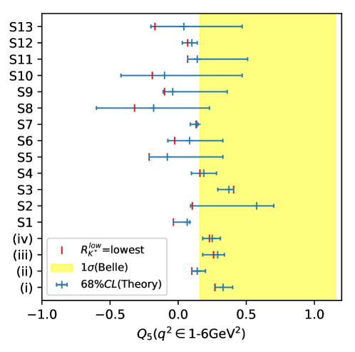
Figure 1: Predicted range of values of $Q_{5}$ for each of the scenarios in Tables 2, 3 and 6, as well as scenarios (i), (ii), (iii) and (iv) [Eqs. (3), (4) and (I)]. The $1\sigma$ range of the present measurement of $Q_{5}$ [Eq. (26)] is superposed.

III.3 LFUV and LFU New Physics

As noted above, $R_{K}$ and $R_{K^{*}}$ are LFUV observables. On the other hand, the processes $B\to K^{*}\mu^{+}\mu^{-}$ and $B_{s}^{0}\to\phi\mu^{+}\mu^{-}$ are governed by $b\to s\mu^{+}\mu^{-}$ transitions. The associated observables are Lepton-Flavour Dependent (LFD). In order to explain the anomalies in $B$ decays, most analyses have assumed NP only in $b\to s\mu^{+}\mu^{-}$, i.e., purely LFUV NP. Recently, in Ref. Alguero:2018nvb , it is suggested to modify the NP paradigm by considering in addition Lepton-Flavour-Universal (LFU) NP. The LFUV observables are then explained by the LFUV NP, while the LFD observables are explained by LFUV $+$ LFU NP. Numerous scenarios are constructed with both LFUV and LFU NP that explain the data as well as scenarios with only LFUV NP.

In Ref. Alguero:2018nvb , the addition of LFU NP was not a necessity, but was seen as a logical possibility. In the present paper, we add NP in $b\to se^{+}e^{-}$ specifically with the aim of improving the explanation of the measured value of $R_{K^{*}}^{low}$. Technically, this is not LFU NP, but it can be made so by including equal WCs in $b\to s\tau^{+}\tau^{-}$ transitions. All our scenarios can be translated into LFUV $+$ LFU NP. Conversely, the scenarios of Ref. Alguero:2018nvb can be translated into $b\to s\mu^{+}\mu^{-}$ NP $+$ $b\to se^{+}e^{-}$ NP. As such, the two papers are complementary to one another.

Here is an example. Ref. Alguero:2018nvb performs the analysis in terms of the LFUV WCs $C^{V}_{i\ell}$ and the LFU WCs $C_{i}^{U}$ ($i=9,10$, $\ell=e,\mu$). Without loss of generality, they set $C^{V}_{ie}=0$. In the most general case, where all four WCs are free, the best-fit values of the WCs are found to be

$$C^{V}_{9\mu}=0.08~{},~{}~{}C^{V}_{10\mu}=1.14~{},~{}~{}C^{U}_{9}=-1.26~{},~{}~{}C^{U}_{10}=-0.91~{}.$$ (28)

Converting these to $b\to s\mu^{+}\mu^{-}$ and $b\to se^{+}e^{-}$ WCs, one obtains

$$C_{9,{\rm NP}}^{\mu\mu}=-1.18~{},~{}~{}C_{10,{\rm NP}}^{\mu\mu}=0.23~{},~{}~{}C_{9,{\rm NP}}^{ee}=-1.26~{},~{}~{}C_{10,{\rm NP}}^{ee}=-0.91~{}.$$ (29)

These are to be compared with the best-fit values of the WCs in scenario S10 of Table 3. The agreement is excellent. We therefore see that our scenario S10 is equivalent to the most general LFUV/LFU scenario of Ref. Alguero:2018nvb . That is, this LFUV/LFU scenario can explain the measured value of $R_{K^{*}}^{low}$.

Now, we have found a number of other scenarios which can account for $R_{K^{*}}^{low}$. However, they involve the WCs $C_{9,{\rm NP}}^{\prime ee}$ and/or $C_{10,{\rm NP}}^{\prime ee}$. In Ref. Alguero:2018nvb , the focus was on LFUV NP only in $C_{9,10,{\rm NP}}^{\mu\mu}$. We have given a motivation for also considering LFUV NP in $C_{9,10,{\rm NP}}^{\prime ee}$. Indeed, from a mdel-building point of view, it is quite natural to have both unprimed and primed NP WCs.

IV Conclusions

There are presently disagreements with the predictions of the SM in the measurements of several observables in $B\to K^{*}\mu^{+}\mu^{-}$ and $B_{s}^{0}\to\phi\mu^{+}\mu^{-}$ decays, and in the LFUV ratios $R_{K}$ and $R_{K^{*}}$. Combining the various $B$ anomalies, analyses find that the net discrepancy with the SM is at the level of 4-6$\sigma$. It is also shown that, by adding NP only to $b\to s\mu^{+}\mu^{-}$, one can get a good fit to the data. However, not all discrepancies are explained: there is still a disagreement of $\mathrel{\raise 1.29167pt\hbox{$>$\kern-7.5pt\lower 4.30554pt\hbox{$\sim$}}}1.7\sigma$ with the measured value of $R_{K^{*}}$ at low values of $q^{2}$. Of course, from the point of view of a global fit, this disagreement is not important. Still, it raises the question: if the true value of $R_{K^{*}}^{low}$ is near its measured value, what can explain it?

If there is NP in $b\to s\mu^{+}\mu^{-}$, it would not be at all surprising if there were also NP in $b\to s\mu^{+}\mu^{-}$. In this paper, we show that, if NP in $b\to se^{+}e^{-}$ transitions is also allowed, one can generate values for $R_{K^{*}}^{low}$ within $\sim 1\sigma$ of its measured value. We have constructed a number of different scenarios (i.e., sets of $b\to s\mu^{+}\mu^{-}$ and $b\to se^{+}e^{-}$ Wilson coefficients) in which this occurs. Some have one NP WC (or combination of WCs) in each of $b\to s\mu^{+}\mu^{-}$ and $b\to se^{+}e^{-}$, and some have more NP WCs (or combinations of WCs) in $b\to s\mu^{+}\mu^{-}$ and/or $b\to se^{+}e^{-}$.

The analysis is done in part using a model-independent, effective-field-theory approach. When one has NP only in $b\to s\mu^{+}\mu^{-}$, a popular choice is $C_{9,{\rm NP}}^{\mu\mu}=-C_{10,{\rm NP}}^{\mu\mu}$, i.e., purely LH NP couplings. We find that, if the NP couplings in $b\to se^{+}e^{-}$ are also purely LH, i.e., $C_{9,{\rm NP}}^{ee}=-C_{10,{\rm NP}}^{ee}$, $R_{K^{*}}^{low}$ can not be explained. $b\to se^{+}e^{-}$ NP couplings involving the RH quarks and/or leptons must be involved.

With NP in both $b\to s\mu^{+}\mu^{-}$ and $b\to se^{+}e^{-}$, one has a better agreement with the data, leading to a bigger pull with respect to the SM. Even so, to get a prediction for $R_{K^{*}}^{low}$ within $\sim 1\sigma$ of its measured value, one has to use $b\to se^{+}e^{-}$ WCs that are not the best-fit values, but rather lie elsewhere within the 68% C.L. region. At the level of the goodness-of-fit, this costs very little: the pull is reduced only by  0.2 (i.e., a few percent).

We also perform the analysis using specific models. We find that, with the addition of $b\to se^{+}e^{-}$ NP couplings, the measured value of $R_{K^{*}}^{low}$ can be explained within a model that includes several different types of leptoquark, or with a model containing a $Z^{\prime}$ gauge boson.

Finally, NP in $b\to se^{+}e^{-}$ is independent of $q^{2}$. For each scenario, we can predict the values of $R_{K^{*}}$ and $R_{K}$ to be found in other $q^{2}$ bins. We also show that a future precise measurement of $Q_{5}\equiv P^{\prime\mu\mu}_{5}-P^{\prime ee}_{5}$ will help in distinguishing the various scenarios. It can also distinguish scenarios with NP only in $b\to s\mu^{+}\mu^{-}$ from those in which NP in $b\to se^{+}e^{-}$ is also present.

Note added: recently, at Moriond 2019, LHCb presented new $R_{K}$ results LHCbRKnew and Belle presented its measurement of $R_{K^{*}}$ BelleRK*new . Following these announcements, global fits using the new data were performed in Refs. Alguero:2019ptt ; Alok:2019ufo ; Ciuchini:2019usw ; Datta:2019zca ; Aebischer:2019mlg ; Kowalska:2019ley , and it was found that the discrepancy with the predictions of the SM is still sizeable. In three of these studies Alguero:2019ptt ; Datta:2019zca ; Aebischer:2019mlg , separate fits to the $b\to s\mu^{+}\mu^{-}$ and $R_{K^{(*)}}$ data were performed. The result was that there is now a tension between these two fits: under the assumption that NP enters only in $b\to s\mu^{+}\mu^{-}$, the best-fit values of the NP WCs differ by $\mathrel{\raise 1.29167pt\hbox{$>$\kern-7.5pt\lower 4.30554pt\hbox{$\sim$}}}1\sigma$. This tension can be removed by also allowing for NP in $b\to se^{+}e^{-}$. In Ref. Datta:2019zca , the additional NP contributions appear only in $b\to se^{+}e^{-}$, while in Refs. Alguero:2019ptt ; Aebischer:2019mlg , lepton-flavour-universal NP contributions to both $b\to s\mu^{+}\mu^{-}$ and $b\to se^{+}e^{-}$ are added.

Acknowledgments: This work was financially supported in part by NSERC of Canada.

References

• (1) R. Aaij et al. [LHCb Collaboration], “Measurement of Form-Factor-Independent Observables in the Decay $B^{0}\to K^{*0}\mu^{+}\mu^{-}$,” Phys. Rev. Lett.  111, 191801 (2013) doi:10.1103/PhysRevLett.111.191801 [arXiv:1308.1707 [hep-ex]].
• (2) R. Aaij et al. [LHCb Collaboration], “Angular analysis of the $B^{0}\to K^{*0}\mu^{+}\mu^{-}$ decay using 3 fb-1 of integrated luminosity,” JHEP 1602, 104 (2016) doi:10.1007/JHEP02(2016)104 [arXiv:1512.04442 [hep-ex]].
• (3) A. Abdesselam et al. [Belle Collaboration], “Angular analysis of $B^{0}\to K^{\ast}(892)^{0}\ell^{+}\ell^{-}$,” arXiv:1604.04042 [hep-ex].
• (4) ATLAS Collaboration, “Angular analysis of $B_{d}^{0}\to K^{*}\mu^{+}\mu^{-}$ decays in $pp$ collisions at $\sqrt{s}=8$ TeV with the ATLAS detector,” Tech. Rep. ATLAS-CONF-2017-023, CERN, Geneva, 2017.
• (5) CMS Collaboration, “Measurement of the $P_{1}$ and $P^{\prime}_{5}$ angular parameters of the decay $B^{0}\to K^{*0}\mu^{+}\mu^{-}$ in proton-proton collisions at $\sqrt{s}=8$ TeV,” Tech. Rep. CMS-PAS-BPH-15-008, CERN, Geneva, 2017.
• (6) R. Aaij et al. [LHCb Collaboration], “Differential branching fraction and angular analysis of the decay $B_{s}^{0}\to\phi\mu^{+}\mu^{-}$,” JHEP 1307, 084 (2013) doi:10.1007/JHEP07(2013)084 [arXiv:1305.2168 [hep-ex]].
• (7) R. Aaij et al. [LHCb Collaboration], “Angular analysis and differential branching fraction of the decay $B^{0}_{s}\to\phi\mu^{+}\mu^{-}$,” JHEP 1509, 179 (2015) doi:10.1007/JHEP09(2015)179 [arXiv:1506.08777 [hep-ex]].
• (8) R. Aaij et al. [LHCb Collaboration], “Test of lepton universality using $B^{+}\rightarrow K^{+}\ell^{+}\ell^{-}$ decays,” Phys. Rev. Lett.  113, 151601 (2014) doi:10.1103/PhysRevLett.113.151601 [arXiv:1406.6482 [hep-ex]].
• (9) R. Aaij et al. [LHCb Collaboration], “Test of lepton universality with $B^{0}\rightarrow K^{*0}\ell^{+}\ell^{-}$ decays,” JHEP 1708, 055 (2017) doi:10.1007/JHEP08(2017)055 [arXiv:1705.05802 [hep-ex]].
• (10) B. Capdevila, A. Crivellin, S. Descotes-Genon, J. Matias and J. Virto, “Patterns of New Physics in $b\to s\ell^{+}\ell^{-}$ transitions in the light of recent data,” JHEP 1801, 093 (2018) doi:10.1007/JHEP01(2018)093 [arXiv:1704.05340 [hep-ph]].
• (11) W. Altmannshofer, P. Stangl and D. M. Straub, “Interpreting Hints for Lepton Flavor Universality Violation,” Phys. Rev. D 96, no. 5, 055008 (2017) doi:10.1103/PhysRevD.96.055008 [arXiv:1704.05435 [hep-ph]].
• (12) G. D’Amico, M. Nardecchia, P. Panci, F. Sannino, A. Strumia, R. Torre and A. Urbano, “Flavor anomalies after the $R_{K^{*}}$ measurement,” JHEP 1709, 010 (2017) doi:10.1007/JHEP09(2017)010 [arXiv:1704.05438 [hep-ph]].
• (13) G. Hiller and I. Nisandzic, “$R_{K}$ and $R_{K^{\ast}}$ beyond the standard model,” Phys. Rev. D 96, no. 3, 035003 (2017) doi:10.1103/PhysRevD.96.035003 [arXiv:1704.05444 [hep-ph]].
• (14) L. S. Geng, B. Grinstein, S. Jäger, J. Martin Camalich, X. L. Ren and R. X. Shi, “Towards the discovery of new physics with lepton-universality ratios of $b\to s\ell\ell$ decays,” Phys. Rev. D 96, no. 9, 093006 (2017) doi:10.1103/PhysRevD.96.093006 [arXiv:1704.05446 [hep-ph]].
• (15) M. Ciuchini, A. M. Coutinho, M. Fedele, E. Franco, A. Paul, L. Silvestrini and M. Valli, “On Flavorful Easter eggs for New Physics hunger and Lepton Flavor Universality violation,” Eur. Phys. J. C 77, no. 10, 688 (2017) doi:10.1140/epjc/s10052-017-5270-2 [arXiv:1704.05447 [hep-ph]].
• (16) A. Celis, J. Fuentes-Martin, A. Vicente and J. Virto, “Gauge-invariant implications of the LHCb measurements on lepton-flavor nonuniversality,” Phys. Rev. D 96, no. 3, 035026 (2017) doi:10.1103/PhysRevD.96.035026 [arXiv:1704.05672 [hep-ph]].
• (17) A. K. Alok, B. Bhattacharya, A. Datta, D. Kumar, J. Kumar and D. London, “New Physics in $b\to s\mu^{+}\mu^{-}$ after the Measurement of $R_{K^{*}}$,” Phys. Rev. D 96, no. 9, 095009 (2017) doi:10.1103/PhysRevD.96.095009 [arXiv:1704.07397 [hep-ph]].
• (18) See, for example, G. Hiller and F. Kruger, “More model-independent analysis of $b\to s$ processes,” Phys. Rev. D 69, 074020 (2004) doi:10.1103/PhysRevD.69.074020 [hep-ph/0310219].
• (19) D. M. Straub, “flavio: a Python package for flavour and precision phenomenology in the Standard Model and beyond,” arXiv:1810.08132 [hep-ph].
• (20) A. Datta, J. Kumar, J. Liao and D. Marfatia, “New light mediators for the $R_{K}$ and $R_{K^{*}}$ puzzles,” Phys. Rev. D 97, no. 11, 115038 (2018) doi:10.1103/PhysRevD.97.115038 [arXiv:1705.08423 [hep-ph]].
• (21) W. Altmannshofer, M. J. Baker, S. Gori, R. Harnik, M. Pospelov, E. Stamou and A. Thamm, “Light resonances and the low-$q^{2}$ bin of ${R}_{K^{*}}$,” JHEP 1803, 188 (2018) doi:10.1007/JHEP03(2018)188 [arXiv:1711.07494 [hep-ph]].
• (22) D. Bardhan, P. Byakti and D. Ghosh, “Role of Tensor operators in $R_{K}$ and $R_{K^{*}}$,” Phys. Lett. B 773, 505 (2017) doi:10.1016/j.physletb.2017.08.062 [arXiv:1705.09305 [hep-ph]].
• (23) The expected precision of future measurements of $b\to se^{+}e^{-}$ observables is given in the talk by Carla Marin Benito, “LHCb: Experimental overview on measurements with rare decays,” at the conference Implications of LHCb measurements and future prospects, October, 2018.
• (24) M. Algueró, B. Capdevila, S. Descotes-Genon, P. Masjuan and J. Matias, “Are we overlooking Lepton Flavour Universal New Physics in $b\to s\ell\ell$ ?,” arXiv:1809.08447 [hep-ph].
• (25) S. Wehle et al. [Belle Collaboration], “Lepton-Flavor-Dependent Angular Analysis of $B\to K^{\ast}\ell^{+}\ell^{-}$,” Phys. Rev. Lett.  118, no. 11, 111801 (2017) doi:10.1103/PhysRevLett.118.111801 [arXiv:1612.05014 [hep-ex]].
• (26) R. Aaij et al. [LHCb Collaboration], “Measurement of the $B^{0}\rightarrow K^{*0}e^{+}e^{-}$ branching fraction at low dilepton mass,” JHEP 1305, 159 (2013) doi:10.1007/JHEP05(2013)159 [arXiv:1304.3035 [hep-ex]].
• (27) R. Aaij et al. [LHCb Collaboration], “Angular analysis of the $B^{0}\to K^{*0}e^{+}e^{−}$ decay in the low-q2 region,” JHEP 1504, 064 (2015) doi:10.1007/JHEP04(2015)064 [arXiv:1501.03038 [hep-ex]].
• (28) J. P. Lees et al. [BaBar Collaboration], “Measurement of the $B\to X_{s}l^{+}l^{-}$ branching fraction and search for direct CP violation from a sum of exclusive final states,” Phys. Rev. Lett.  112, 211802 (2014) doi:10.1103/PhysRevLett.112.211802 [arXiv:1312.5364 [hep-ex]].
• (29) M. Bordone, G. Isidori and A. Pattori, “On the Standard Model predictions for $R_{K}$ and $R_{K^{*}}$,” Eur. Phys. J. C 76, no. 8, 440 (2016) doi:10.1140/epjc/s10052-016-4274-7 [arXiv:1605.07633 [hep-ph]].
• (30) W. Altmannshofer, C. Niehoff, P. Stangl and D. M. Straub, “Status of the $B\rightarrow K^{*}\mu^{+}\mu^{-}$ anomaly after Moriond 2017,” Eur. Phys. J. C 77, no. 6, 377 (2017) doi:10.1140/epjc/s10052-017-4952-0 [arXiv:1703.09189 [hep-ph]].
• (31) R. Alonso, B. Grinstein and J. Martin Camalich, “Lepton universality violation and lepton flavor conservation in $B$-meson decays,” JHEP 1510, 184 (2015) doi:10.1007/JHEP10(2015)184 [arXiv:1505.05164 [hep-ph]].
• (32) Y. Sakaki, R. Watanabe, M. Tanaka and A. Tayduganov, “Testing leptoquark models in $\bar{B}\to D^{(*)}\tau\bar{\nu}$,” Phys. Rev. D 88, no. 9, 094012 (2013) doi:10.1103/PhysRevD.88.094012 [arXiv:1309.0301 [hep-ph]].
• (33) For example, see A. K. Alok, B. Bhattacharya, D. Kumar, J. Kumar, D. London and S. U. Sankar, “New physics in $b\rightarrow s\mu^{+}\mu^{-}$: Distinguishing models through CP-violating effects,” Phys. Rev. D 96, no. 1, 015034 (2017) doi:10.1103/PhysRevD.96.015034 [arXiv:1703.09247 [hep-ph]].
• (34) For example, see A. K. Alok, A. Datta, A. Dighe, M. Duraisamy, D. Ghosh and D. London, “New Physics in $b\to s\mu^{+}\mu^{-}$: CP-Conserving Observables,” JHEP 1111, 121 (2011) doi:10.1007/JHEP11(2011)121 [arXiv:1008.2367 [hep-ph]].
• (35) R. Aaij et al. [LHCb Collaboration], “Measurement of the $B^{0}_{s}\to\mu^{+}\mu^{-}$ branching fraction and search for $B^{0}\to\mu^{+}\mu^{-}$ decays at the LHCb experiment,” Phys. Rev. Lett.  111, 101805 (2013) doi:10.1103/PhysRevLett.111.101805 [arXiv:1307.5024 [hep-ex]].
• (36) V. Khachatryan et al. [CMS and LHCb Collaborations], “Observation of the rare $B^{0}_{s}\to\mu^{+}\mu^{-}$ decay from the combined analysis of CMS and LHCb data,” Nature 522, 68 (2015) doi:10.1038/nature14474 [arXiv:1411.4413 [hep-ex]].
• (37) M. Tanabashi et al. [Particle Data Group], “Review of Particle Physics,” Phys. Rev. D 98, no. 3, 030001 (2018). doi:10.1103/PhysRevD.98.030001
• (38) A. Crivellin, D. Müller, A. Signer and Y. Ulrich, “Correlating lepton flavor universality violation in $B$ decays with $\mu\to e\gamma$ using leptoquarks,” Phys. Rev. D 97, no. 1, 015019 (2018) doi:10.1103/PhysRevD.97.015019 [arXiv:1706.08511 [hep-ph]].
• (39) B. Aubert et al. [BaBar Collaboration], “Measurements of branching fractions, rate asymmetries, and angular distributions in the rare decays $B\to K\ell^{+}\ell^{-}$ and $B\to K^{*}\ell^{+}\ell^{-}$,” Phys. Rev. D 73, 092001 (2006) doi:10.1103/PhysRevD.73.092001 [hep-ex/0604007].
• (40) R. Aaij et al. [LHCb Collaboration], “Search for the lepton-flavour violating decays B${}_{(s)}^{0}\to e^{\pm}\mu^{\mp}$,” JHEP 1803, 078 (2018) doi:10.1007/JHEP03(2018)078 [arXiv:1710.04111 [hep-ex]].
• (41) J. Kumar, D. London and R. Watanabe, “Combined Explanations of the $b\to s\mu^{+}\mu^{-}$ and $b\to c\tau^{-}{\bar{\nu}}$ Anomalies: a General Model Analysis,” arXiv:1806.07403 [hep-ph].
• (42) A. Crivellin, L. Hofer, J. Matias, U. Nierste, S. Pokorski and J. Rosiek, “Lepton-flavour violating $B$ decays in generic $Z^{\prime}$ models,” Phys. Rev. D 92, no. 5, 054013 (2015) doi:10.1103/PhysRevD.92.054013 [arXiv:1504.07928 [hep-ph]].
• (43) D. Guadagnoli, M. Reboud and O. Sumensari, “A gauged horizontal $SU(2)$ symmetry and $R_{K^{(\ast)}}$,” arXiv:1807.03285 [hep-ph].
• (44) S. Descotes-Genon, L. Hofer, J. Matias and J. Virto, “Global analysis of $b\to s\ell\ell$ anomalies,” JHEP 1606, 092 (2016) doi:10.1007/JHEP06(2016)092 [arXiv:1510.04239 [hep-ph]].
• (45) T. Humair (for the LHCb Collaboration), “Lepton Flavor Universality tests with heavy flavour decays at LHCb,” talk given at Moriond, March 22 2019. See also R. Aaij et al. [LHCb Collaboration], “Search for lepton-universality violation in $B^{+}\to K^{+}\ell^{+}\ell^{-}$ decays,” arXiv:1903.09252 [hep-ex].
• (46) M. Prim (for the Belle Collaboration), “Search for $B\to\ell\nu\gamma$ and $B\to\mu\nu_{\mu}$ and Test of Lepton Universality with $R(K^{*})$ at Belle,” talk given at Moriond, March 22 2019. See also A. Abdesselam et al. [Belle Collaboration], “Test of lepton flavor universality in ${B\to K^{\ast}\ell^{+}\ell^{-}}$ decays at Belle,” arXiv:1904.02440 [hep-ex].
• (47) M. Algueró, B. Capdevila, A. Crivellin, S. Descotes-Genon, P. Masjuan, J. Matias and J. Virto, “Addendum: “Patterns of New Physics in $b\to s\ell^{+}\ell^{-}$ transitions in the light of recent data” and “Are we overlooking Lepton Flavour Universal New Physics in $b\to s\ell\ell\,$?”,” arXiv:1903.09578 [hep-ph].
• (48) A. K. Alok, A. Dighe, S. Gangal and D. Kumar, “Continuing search for new physics in $b\to s\mu\mu$ decays: two operators at a time,” arXiv:1903.09617 [hep-ph].
• (49) M. Ciuchini, A. M. Coutinho, M. Fedele, E. Franco, A. Paul, L. Silvestrini and M. Valli, “New Physics in $b\to s\ell^{+}\ell^{-}$ confronts new data on Lepton Universality,” arXiv:1903.09632 [hep-ph].
• (50) A. Datta, J. Kumar and D. London, “The $B$ Anomalies and New Physics in $b\to se^{+}e^{-}$,” arXiv:1903.10086 [hep-ph].
• (51) J. Aebischer, W. Altmannshofer, D. Guadagnoli, M. Reboud, P. Stangl and D. M. Straub, “$B$-decay discrepancies after Moriond 2019,” arXiv:1903.10434 [hep-ph].
• (52) K. Kowalska, D. Kumar and E. M. Sessolo, “Implications for New Physics in $b\to s\mu\mu$ transitions after recent measurements by Belle and LHCb,” arXiv:1903.10932 [hep-ph].