Orion SrcI’s disk is salty

Abstract

We report the detection of NaCl, KCl, and their ³⁷Cl and ⁴¹K isotopologues toward the disk around Orion SrcI. About 60 transitions of these molecules were identified. This is the first detection of these molecules in the interstellar medium not associated with the ejecta of evolved stars. It is also the first ever detection of the vibrationally excited states of these lines in the ISM above $v=1$, with firm detections up to $v=6$. The salt emission traces the region just above the continuum disk, possibly forming the base of the outflow. The emission from the vibrationally excited transitions is inconsistent with a single temperature, implying the lines are not in LTE. We examine several possible explanations of the observed high excitation lines, concluding that the vibrational states are most likely to be radiatively excited via rovibrational transitions in the 25-35 $\mu\textrm{m}$ (NaCl) and 35-45 $\mu\textrm{m}$ (KCl) range. We suggest that the molecules are produced by destruction of dust particles. Because these molecules are so rare, they are potentially unique tools for identifying high-mass protostellar disks and measuring the radiation environment around accreting young stars.

doublespace

1 Introduction

The disk around Orion Source I (SrcI) has been the subject of intense study, as it is the closest ($d\approx 400$ pc; Grossschedl et al., 2018) disk around a ‘high-mass’ ($M>8$ $M_{\odot}$) star (Hirota et al., 2014; Plambeck & Wright, 2016; Ginsburg et al., 2018). It is also in many ways a unique source, being the only known protostellar object with both SiO and H₂O masers in an outflow (Plambeck et al., 2009; Goddi et al., 2009; Matthews et al., 2010; Goddi et al., 2010; Niederhofer et al., 2012; Greenhill et al., 2013). In Ginsburg et al. (2018), a subset of the authors reported 0.03$\arcsec$ ALMA observations of SrcI that allowed a measurement of the outer rotation curve of the 5(5,0)-6(4,3) H₂O line in the disk and along the base of the outflow; these measurements showed that the interior mass was $15\pm 2$ $M_{\odot}$. In the same data, we found additional emission lines that closely traced the disk and its Keplerian rotation curve, but were unable to identify the molecular species responsible for these lines. We now identify them as transitions of NaCl, KCl, and their isotopologues, many in excited vibrational levels.

Disks are ubiquitous around forming stars of any mass. They provide the main mechanism for mediating accretion, and, via outflows, shedding angular momentum from the system. Despite their theoretical importance, the role of disks in high-mass star formation remains observationally uncertain, since the only definitive disk detections are around stars that have already acquired most of their mass (e.g., Girart et al., 2017). The lack of clear disk detections is, at least in part, because there were no known spectral lines that trace a disk and not the molecule-rich “hot core” in the surrounding region (Goddi et al., 2018; Cesaroni et al., 2017). For low-mass sources, where the disks are observed in isolation after the surrounding core has accreted or dispersed, this ambiguity is absent. For high-mass sources, which evolve so quickly that the disks are still embedded in their natal hot core, substantial confusion can arise. Further complicating matters, the large amount of dust in these dense regions may obscure the disks at wavelengths shorter than 3 mm.

While dozens of species have been detected in the disks around low-mass stars (McGuire, 2018), these molecules are comprised solely of a small selection of elements: H, C, N, O, and S. All of the molecules seen in disks are also prevalent in the ISM, particularly in the hot cores surrounding high-mass stars (Nummelin et al., 1998; Belloche et al., 2013). In high-mass environments, this therefore limits their utility as unique disk tracers, hiding the kinematic signatures of rotation.

Molecules consisting of alkali metals and halogens have only rarely been detected in space (McGuire, 2018). Because of their rarity, their use as a diagnostic tool to measure metallicity and local physical conditions has been limited. However, some of these molecules, such as KCl and NaCl, have a rich spectrum with dozens of lines arising in a single observing band so they have great potential to probe either local gas properties or the radiation field when they are detected.

KCl and NaCl have so far been observed toward evolved stars including the carbon star IRC +10216 (Cernicharo & Guelin, 1987), the oxygen-rich evolved stars IK Tauri and VY Canis Majoris (Milam et al., 2007), the post-AGB star envelope CRL 2688 (Highberger et al., 2003), and the AGB star wind around OH 231+4.2 (Sánchez Contreras et al., 2018). In these sources, they exist only in a limited range of radii from the central star as they are carried outward in slow winds (Herwig, 2005). The limited environments in which these molecules have been detected suggests that they persist in the gas phase for only a brief period before they are incorporated into dust grains. This transient gas-phase abundance is analogous to that which makes SiO an excellent tracer of recent shock events: Si is sputtered from grains into the gas phase where it reacts with oxygen to form SiO. Further reactions rapidly form SiO₂, depleting the gas-phase SiO abundance, and making that molecule an indicator of a recent shock (Schilke et al., 1997).

If the production pathways, and role of the physical environment on those pathways, can be constrained for NaCl and KCl, the presence of these molecules has the potential to be a powerful tracer of gas physical conditions and history. The rarity of these molecules in the ISM makes them a uniquely powerful tracer when they can be found. Below, we describe the first detection of salts in a high-mass protostellar disk, unveiling what may be the only molecules that specifically trace disks around high-mass stars.

2 Observations and Analysis

The observations presented here are described in Ginsburg et al. (2018) as part of ALMA project 2016.1.00165.S. We use the robust 0.5 weighted spectral cubes from all three bands (B3 3.0 mm, B6 1.3 mm, B7 0.87 mm) for our spectroscopic analysis.

Appendix D of that paper describes the spectral extraction method, which we summarize here. We used the U232.511 line (which we now identify as NaCl v=1 J=18-17) to find the velocity centroid for each (spatial) pixel across the SrcI disk. We shifted the spectrum along each such pixel to 0 km s^-1, then averaged the shifted spectra over the region with significant emission in the NaCl line. The averaging area is approximately the extent of the continuum disk, 0.03 square arcseconds, or about 4, 20, and 40 beam areas, resulting in an improvement in the signal-to-noise of about $2\times$, $4\times$, and $6\times$ respectively in Band 3, 6, and 7. This stacked spectrum, shown in Figures 1-3, traces material just above and below the optically thick continuum disk (Figure 4). Because this procedure removes the rotational velocity field of the disk, lines in the stacked spectrum are narrower than one would observe in a lower spatial resolution observation of the disk. One may think of the stacked spectrum as the output of a matched filter that is optimized for detection of disk emission.

In the appendix of Ginsburg et al. (2018), we listed over 20 unidentified lines in the B6 ALMA spectra, and commented that “there is no consistent pattern to the detected lines and no individual species can explain more than a few of the observed lines.” This statement was incorrect, as there are obvious carriers for the majority of the unidentified lines that we had simply overlooked: NaCl, KCl, and their isotopologues. The detected lines have amplitudes in the range 0.5-3 mJy $\textrm{beam}^{-1}$, corresponding to brightness temperatures 5-20 K.

In Figures 1-3, we have labeled all of the detections and marginal detections of salt lines, as well as the most prominent outflow (e.g., SiO and H₂O) lines. Only 2-3 emission lines are now unidentified in the B6 and B7 spectra, though there are over a dozen in B3 that we have not identified.

We also tentatively identify broad lines at 229.7 GHz and 344.4 GHz as AlO. If the identification is correct, these lines are broad because of the rich hyperfine spectrum of AlO.

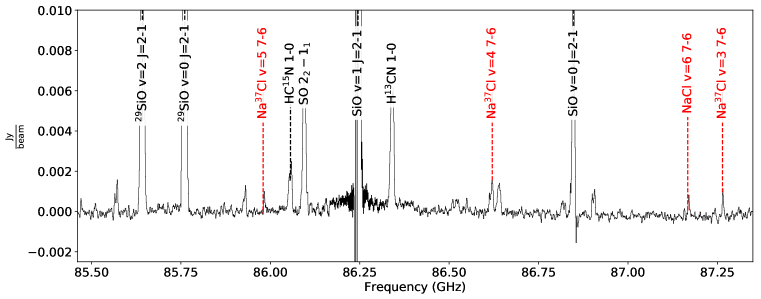
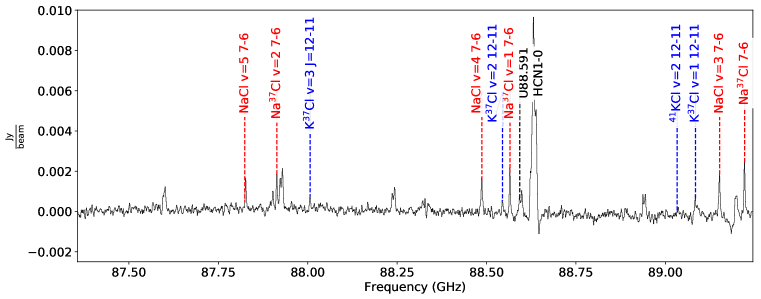
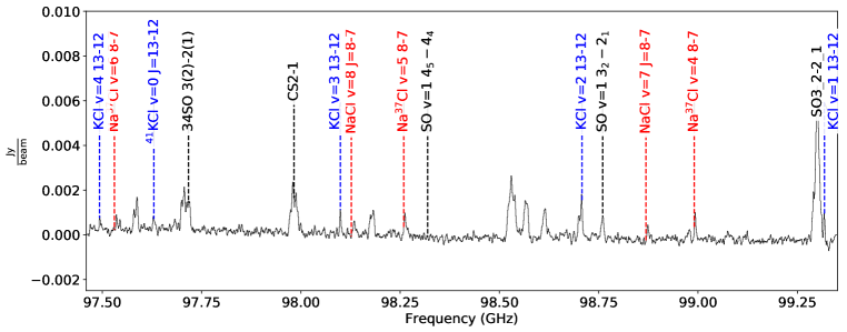
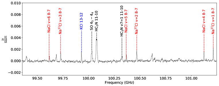
Figure 1: Stacked spectra from the Band 3 setup (see Section 2).

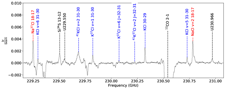
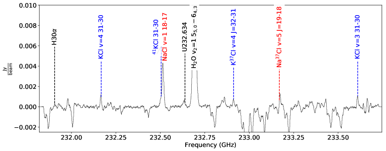
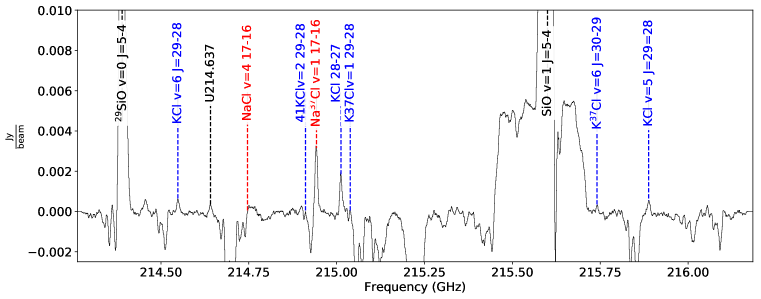
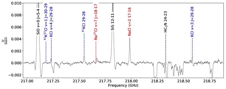
Figure 2: Stacked spectra from the Band 6 setup (see Section 2).

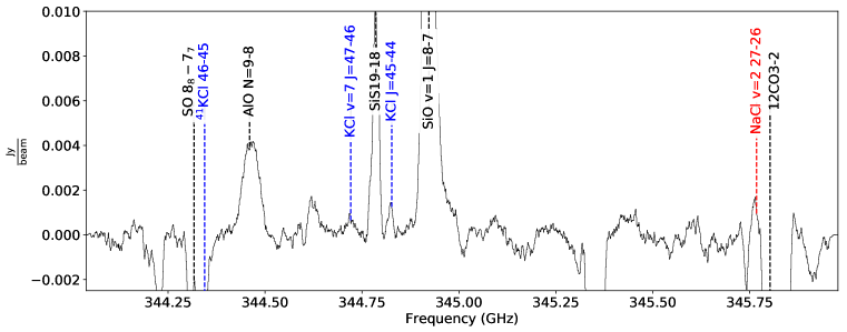
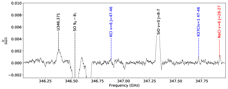
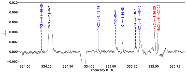
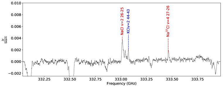
Figure 3: Stacked spectra from the Band 7 setup (see Section 2).

In Tables 1-6, we list all of the salt lines in vibrational energy levels up to v=8 that lie within our observed bands and whether or not they were detected. We employ the following flag scheme: ‘D’ for detection, ‘N’ for nondetection, ‘Q’ for questionable (e.g., low signal-to-noise, but possibly detected, or in regions where the noise is not Gaussian and may be affected by other lines). We additionally include a flag ‘C’ for ‘confused’, which we add to the flag string if the line is blended with another brighter line of a different species. There are robust detections of about 60 lines, up to the v=6 vibrational level.

The majority of the NaCl and KCl lines that we detected are in excited vibrational states. Although transitions in higher vibrational states were measured, and some reported, in Caris et al. (2004), they did not provide the complete catalogs needed for this analysis, nor to our knowledge are these catalogues available in any of the standard online databases (i.e., CDMS, SLAIM, JPL; Müller et al., 2005; Lovas et al., 2005; Pickett et al., 1998). We obtained the KCl frequencies for these lines from the catalogs of Barton et al. (2014), which was designed primarily for use in exoplanet atmospheres and includes over 10⁵ transitions for each molecular species and isotopologue with levels up to $E_{U}\sim 5\times 10^{4}$ K, and the NaCl frequencies from Cabezas et al. (2016), who provided more accurate potential energy and dipole moment functions. The primary result of these catalogs for the purposes of this work is the prediction of frequencies in vibrational states higher than those measured in the laboratory.

In using these catalogs, we found a systematic discrepancy between the rest frequencies reported by Barton et al. (2014), and those given by Caris et al. (2004) and Caris et al. (2002): the KCl lines appear to be systematically offset by $\sim$15-20 km s^-1 in the Barton catalog. The Barton data are also discrepant with the more recent Cabezas et al. (2016) work that cataloged only NaCl lines. The offset is a function of the vibrational and rotational energy states, indicating that it resulted from an incorrect rotational and/or distortion constant. We correct for this error by performing a bilinear fit in frequency as a function of $v_{u}$ and $J_{u}$. In the transitions available in both catalogs the resulting frequency differences are generally $<0.1$ km s^-1, which is more than sufficient for a reliable match to our spectra. We then applied these fitted models to the higher-$v$ states tabulated by Barton to get corrected rest frequencies for KCl, while for NaCl we used the Cabezas et al. (2016) values. We note that the values printed in Barton et al. (2014) differ from those in the digital catalogs hosted on exomol.com, so we suspect the error was merely a transcription error of some sort.

Table 1: All cataloged NaCl lines in the Band 3 tuning

Na Isotope	Cl Isotope	v	Ju	Jl	EU	Aul	Frequency	Flag
23	35	8	7	6	4035.4	0.00031	85.87018	N
23	37	5	7	6	2538.2	0.00030	85.98167	D
23	35	7	7	6	3550.1	0.00031	86.51754	Q
23	37	4	7	6	2043.6	0.00030	86.62109	D
23	35	6	7	6	3060.0	0.00032	87.16921	D
23	37	3	7	6	1544.3	0.00030	87.26464	D
23	35	5	7	6	2565.2	0.00032	87.82519	D
23	37	2	7	6	1040.1	0.00031	87.91232	D
23	35	4	7	6	2065.5	0.00032	88.48549	D
23	37	1	7	6	531.1	0.00031	88.56415	D
23	35	3	7	6	1561.0	0.00033	89.15011	D
23	37	0	7	6	17.1	0.00031	89.22011	D
23	37	6	8	7	3032.7	0.00045	97.53449	Q
23	35	8	8	7	4040.1	0.00047	98.13295	Q
23	37	5	8	7	2542.9	0.00045	98.26052	Q
23	35	7	8	7	3554.8	0.00047	98.87277	Q
23	37	4	8	7	2048.4	0.00045	98.99127	D
23	35	6	8	7	3064.8	0.00048	99.61753	D
23	37	3	8	7	1549.1	0.00046	99.72675	D
23	35	5	8	7	2570.0	0.00048	100.36722	D
23	37	2	8	7	1045.0	0.00046	100.46695	D
23	35	4	8	7	2070.4	0.00048	101.12183	D
23	37	1	8	7	536.0	0.00047	101.21188	D

Table 2: All cataloged NaCl lines in the Band 6 tuning

Na Isotope	Cl Isotope	v	Ju	Jl	EU	Aul	Frequency	Flag
23	35	4	17	16	2141.3	0.00480	214.74232	CN
23	37	1	17	16	607.0	0.00460	214.93871	D
23	37	8	18	17	4076.0	0.00520	216.05316	N
23	37	7	18	17	3596.2	0.00520	217.66504	Q
23	35	2	17	16	1128.4	0.00490	217.98023	D
23	37	0	18	17	104.6	0.00550	229.24605	D
23	37	7	19	18	3607.2	0.00610	229.73281	CN
23	35	2	18	17	1139.5	0.00580	230.77917	D
23	35	1	18	17	625.7	0.00580	232.50998	D
23	35	8	19	18	4130.7	0.00650	232.85904	Q
23	37	5	19	18	2633.6	0.00620	233.16920	CD

Table 3: All cataloged NaCl lines in the Band 7 tuning

Na Isotope	Cl Isotope	v	Ju	Jl	EU	Aul	Frequency	Flag
23	35	2	26	25	1250.2	0.01800	333.00729	D
23	35	7	27	26	3757.5	0.01900	333.03612	CQ
23	37	4	27	26	2251.3	0.01800	333.45906	D
23	35	1	26	25	737.2	0.01800	335.50656	D
23	35	6	27	26	3269.0	0.01900	335.54793	CQ
23	37	8	28	27	4211.3	0.02000	335.63074	CN
23	35	7	28	27	3774.1	0.02100	345.31422	CN
23	37	4	28	27	2267.9	0.02000	345.75480	CN
23	35	2	27	26	1266.8	0.02000	345.76204	CD
23	37	8	29	28	4228.0	0.02200	347.55955	N
23	35	6	28	27	3285.7	0.02100	347.91891	NC

Table 4: All cataloged KCl lines in the Band 3 tuning

K Isotope	Cl Isotope	v	Ju	Jl	EU	Aul	Frequency	Flag
41	35	8	12	11	3092.4	0.00041	85.80766	N
39	37	7	12	11	2713.3	0.00041	85.87379	N
41	37	3	12	11	1183.9	0.00039	85.93776	N
41	35	7	12	11	2720.7	0.00042	86.33986	CN
39	37	6	12	11	2339.4	0.00041	86.40364	N
41	37	2	12	11	801.6	0.00039	86.45668	N
41	35	6	12	11	2345.7	0.00042	86.87413	N
39	37	5	12	11	1962.2	0.00042	86.93553	N
41	37	1	12	11	416.1	0.00040	86.97743	Q
41	35	5	12	11	1967.6	0.00042	87.41041	N
39	37	4	12	11	1581.9	0.00042	87.46938	N
41	37	0	12	11	27.3	0.00040	87.50010	Q
39	35	8	12	11	3127.7	0.00044	87.77742	N
41	35	4	12	11	1586.3	0.00043	87.94866	N
39	37	3	12	11	1198.3	0.00042	88.00523	D
39	35	7	12	11	2751.8	0.00045	88.32895	Q
41	35	3	12	11	1201.7	0.00043	88.48896	CQ
39	37	2	12	11	811.5	0.00042	88.54307	D
39	35	6	12	11	2372.8	0.00045	88.88253	N
41	35	2	12	11	813.8	0.00043	89.03129	D
39	37	1	12	11	421.4	0.00043	89.08292	D
39	35	4	13	12	1609.5	0.00058	97.49133	D
41	35	0	13	12	32.8	0.00056	97.62809	D
41	37	7	14	13	2690.7	0.00061	97.85364	N
39	35	3	13	12	1220.6	0.00059	98.09753	D
41	37	6	14	13	2321.0	0.00061	98.44993	N
39	35	2	13	12	828.3	0.00059	98.70595	D
41	37	5	14	13	1948.2	0.00062	99.04845	N
39	35	1	13	12	432.6	0.00059	99.31663	D
39	37	8	14	13	3093.3	0.00065	99.56276	N
41	37	4	14	13	1572.3	0.00062	99.64924	N
39	35	0	13	12	33.6	0.00060	99.92952	D
41	35	8	14	13	3101.7	0.00066	100.10138	N
39	37	7	14	13	2722.6	0.00065	100.17822	N
41	37	3	14	13	1193.2	0.00063	100.25229	N
41	35	7	14	13	2730.0	0.00067	100.72190	N
39	37	6	14	13	2348.7	0.00066	100.79603	Q
41	37	2	14	13	810.9	0.00063	100.85758	N

Table 5: All cataloged KCl lines in the Band 6 tuning

K Isotope	Cl Isotope	v	Ju	Jl	EU	Aul	Frequency	Flag
39	37	7	30	29	2846.1	0.00654	214.41527	N
39	35	6	29	28	2499.6	0.00648	214.54412	D
41	37	3	30	29	1316.8	0.00626	214.57918	N
41	35	2	29	28	940.8	0.00622	214.90740	CQ
39	35	0	28	27	149.7	0.00609	215.00828	D
39	37	1	29	28	548.5	0.00616	215.03464	CQ
41	37	8	31	30	3187.6	0.00668	215.09368	CN
41	35	7	30	29	2854.2	0.00665	215.57755	CN
39	37	6	30	29	2473.0	0.00659	215.73679	D
41	37	2	30	29	935.3	0.00631	215.87559	N
39	35	5	29	28	2118.0	0.00653	215.88373	D
39	37	5	30	29	2096.7	0.00664	217.06391	Q
41	37	1	30	29	550.6	0.00635	217.17723	Q
39	35	4	29	28	1733.2	0.00658	217.22891	CD
41	35	0	29	28	156.7	0.00631	217.54317	D
41	37	6	31	30	2452.9	0.00677	217.72366	N
41	35	5	30	29	2102.8	0.00675	218.24805	N
39	37	4	30	29	1717.2	0.00668	218.39657	CN
41	37	0	30	29	162.6	0.00639	218.48414	CN
39	35	3	29	28	1345.1	0.00662	218.57971	D
39	35	6	31	30	2521.2	0.00793	229.29217	CD
41	35	2	31	30	962.5	0.00761	229.68227	CD
39	37	1	31	30	570.2	0.00753	229.81880	D
41	35	7	32	31	2875.9	0.00808	229.90046	Q
39	37	6	32	31	2494.7	0.00800	230.07072	D
41	37	2	32	31	957.1	0.00766	230.22070	Q
41	37	7	33	32	2843.6	0.00812	230.31852	CN
39	35	0	30	29	171.4	0.00749	230.32064	D
39	35	5	31	30	2139.8	0.00798	230.72399	D
39	35	4	31	30	1755.1	0.00804	232.16185	D
41	35	0	31	30	178.7	0.00771	232.49980	CN
41	35	5	32	31	2124.8	0.00819	232.74872	Q
39	37	4	32	31	1739.2	0.00812	232.90755	D
41	37	0	32	31	184.6	0.00777	233.00319	CN
41	37	5	33	32	2102.9	0.00823	233.12954	CN
39	35	3	31	30	1367.1	0.00810	233.60570	D
39	35	8	32	31	3285.5	0.00860	233.72540	N

Table 6: All cataloged KCl lines in the Band 7 tuning

K Isotope	Cl Isotope	v	Ju	Jl	EU	Aul	Frequency	Flag
39	37	5	46	45	2310.3	0.02398	332.14436	CN
39	35	6	45	44	2712.4	0.02429	332.22193	CQ
41	37	8	48	47	3413.8	0.02483	332.29761	N
41	37	1	46	45	764.4	0.02295	332.34847	N
41	35	2	45	44	1154.0	0.02331	332.81369	N
39	37	1	45	44	761.8	0.02309	333.01833	CN
39	35	2	44	43	1155.3	0.02336	333.06770	D
39	37	8	47	46	3441.9	0.02504	333.10414	N
41	37	4	47	46	1921.1	0.02398	333.43025	N
41	35	5	46	45	2317.6	0.02438	333.95245	N
39	37	4	46	45	1932.1	0.02415	334.18696	N
39	35	5	45	44	2332.2	0.02446	334.29930	D
41	37	7	48	47	3049.3	0.02501	334.32791	CD
41	37	0	46	45	377.7	0.02311	334.35249	CN
41	35	1	45	44	764.9	0.02347	334.85439	D
41	35	8	47	46	3452.1	0.02545	334.89960	N
39	37	0	45	44	370.4	0.02325	335.05072	D
39	35	1	44	43	761.7	0.02353	335.13396	D
39	37	7	47	46	3073.3	0.02522	335.16416	Q
39	35	8	46	45	3479.1	0.02557	335.33093	CQ
41	37	3	47	46	1544.2	0.02414	335.45237	N
41	35	7	48	47	3099.1	0.02730	344.08981	CN
41	35	0	46	45	389.0	0.02525	344.33834	CN
39	37	6	48	47	2718.1	0.02705	344.35234	CN
41	37	2	48	47	1180.5	0.02589	344.60998	CQ
39	35	7	47	46	3122.1	0.02747	344.71476	D
39	35	0	45	44	381.2	0.02534	344.82061	D
41	35	3	47	46	1572.6	0.02637	345.37541	CN
41	37	5	49	48	2327.8	0.02698	345.40918	CN
39	37	2	47	46	1182.6	0.02612	345.59885	CN
39	35	3	46	45	1578.4	0.02650	345.94809	CN
41	35	6	48	47	2726.5	0.02750	346.22022	N
39	37	5	48	47	2343.3	0.02724	346.47449	N
41	37	1	48	47	797.3	0.02607	346.69248	CN
39	35	6	47	46	2745.3	0.02767	346.87489	D
39	37	8	49	48	3474.8	0.02837	347.16340	N
41	35	2	47	46	1187.0	0.02655	347.49773	Q
41	37	4	49	48	1954.1	0.02717	347.50839	N
39	37	1	47	46	794.8	0.02630	347.71265	D

We have fit Gaussian line profiles to each of the transitions we flagged as ‘detected’ in Tables 1-6. The fits are reported in Tables 7-12. A few of the integrated intensities (e.g., for the KCl v=5 45-44 line) are discrepantly high compared to transitions at similar $v$ and $J$ states, suggesting that they are blends with other species as denoted in Tables 1-6.

3 Discussion

NaCl and KCl have only been seen in a handful of other sources, all of which were moderately high-mass evolved stars blowing off their envelopes. The known detections include the carbon star envelope IRC +10216 (Cernicharo & Guelin, 1987; Agúndez et al., 2012; Zack et al., 2011), the post-AGB star envelope CRL 2688 (Highberger et al., 2003), and the oxygen-rich evolved star envelopes of VY Canis Majoris and IK Tauri (Milam et al., 2007; Kamiński et al., 2013). To our knowledge, SrcI is only the fifth astronomical source in which KCl and NaCl have been detected. The only previous detections of vibrationally excited NaCl were in the v=1 level in IRC+10216 (Quintana-Lacaci et al., 2016) and VY CMa (Decin et al., 2016), while SrcI exhibits clear emission up to v=6 in both NaCl and KCl.

In these evolved stars, v=0 rotational transitions of NaCl were observed with rotational temperatures ${T_{rot}\sim 70-100}$ K (IK Tau, VY CMa), inferred local temperatures of $\sim 200$ K in shocks (CRL 2688), and $T\approx 700$ K in an expanding shell (IRC+10216). Below, we attempt to determine the physical conditions in the SrcI salt emission regions.

3.1 Spatial distribution of the salt emission

In SrcI, the salt lines originate from the surface layers of the disk (the Band 7 lines exhibit NaCl emission peaks at $\pm 0.032\arcsec=13$ AU above the disk), unlike SiO and H₂O that both exhibit high vertical extents consistent with outflow (Ginsburg et al., 2018). No emission in the salt lines is observed toward the optically thick continuum in the disk midplane (Figure 4). Ginsburg et al. (2018) modeled the line emission now assigned to these salts as a truncated Keplerian disk, finding that the radial distribution of the emission has an inner cutoff $\approx 35-40$ AU and an outer cutoff $\approx 55-60$ AU.

The equilibrium temperature in this radius range can be computed assuming the central source has a luminosity $L=10^{4}L_{\odot}=4\pi r^{2}\sigma_{SB}T^{4}$ ($T_{*}=4000$ K, $R_{*}=210$ $R_{\odot}$), where we solve for temperature with $r$ at the inner and outer radius, giving $T_{eq}=500-670$ K for $r=35-60$ AU, assuming the disk intercepts all of the starlight at this radius. More realistically, providing the opposite limiting case, $T_{eq}=120-180$ K for a flat disk (Eqn. 4 of Chiang & Goldreich, 1997). These cooler temperatures are consistent with the observed brightness temperatures in the outer part of the continuum disk (in Figure 4, the Band 6 and 7 NaCl emission begins just beyond the $T=300$ K continuum contour), although the temperature in the inner portion of the disk reaches $\gtrsim 500$ K.

Figure 4: Peak intensity images of NaCl lines in each band showing the spatial distribution of the emission. From left to right, the lines are: 87.26 GHz NaCl v=3 J=7-6, 232.51 GHz NaCl v=1 J=18-17, and 333.01 GHz NaCl v=2 J=26-25. These are the brightest uncontaminated lines in each of their observing bands. The red contours show the Band 6 226 GHz continuum at levels of 50, 300, and 500 K. White contours are shown at 50 and 100 K (left), 50, 100, 150, and 200 K (center), and 150, 250, and 350 K (right). The red and blue ellipses show the beams for the continuum and the line emission, respectively. The beam sizes are $0.10\arcsec\times 0.08\arcsec$, PA $40.6^{\circ}$, $0.043\arcsec\times 0.034\arcsec$, PA $-87.4^{\circ}$, and $0.029\arcsec\times 0.022\arcsec$, PA $-54.6^{\circ}$, respectively.

We also compare the salt emission locations to the SiO emission regions. Figure 5 shows the SiO v=0 J=8-7 line, which is thermally excited (it shows no sign of masing at any velocity) and traces the outflow. The SiO v=5 J=8-7 line, with an upper state energy level of 8747 K, is also shown. It clearly traces a smaller radius than the NaCl line, but a similar height in the disk. By contrast, the SiO v=0 J=8-7 emission, with $E_{U}=75$ K, starts above the vertical centroid of the NaCl line. These spatial anticorrelations suggest that the difference between the molecules’ emission patterns is driven partly by excitation, since the salt lines have upper state energy levels intermediate between the SiO v=0 and v=5 states and trace an intermediate region.

Figure 5: Peak intensity map of SiO v=0 J=8-7 (gray scale), NaCl v=2 J=26-25 (red contour; 200 K) and SiO v=5 J=8-7 (blue contours; 300, 400, 500, and 600 K). The blue contours in the upper-left come from a blend with a different line.

3.2 Excitation

The detection of vibrationally excited transitions from v=0 to v=6 at similar brightness suggests that the vibrational excitation temperature $T_{ex,vib}$ of the molecules is high. However, we see sharply decreasing populations in the higher rotational levels, indicating a much lower $T_{ex,rot}$.

Within each vibrational state for which we observed several transitions, we attempt to measure a rotational temperature. For the KCl v=0 state, in which we have detected 4 rotational transitions from $30<E_{U}<400$ K, the best fit is $T_{rot}\sim 105$ K (Figure 6). At such a low temperature, the populations of the vibrationally excited states should be effectively zero.

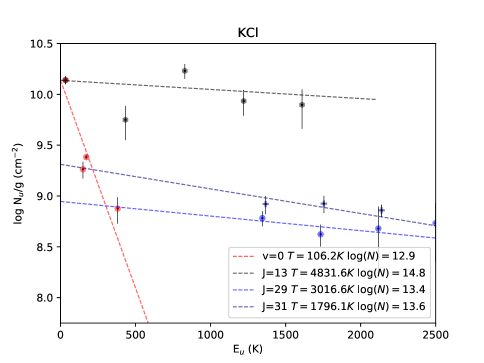
Figure 6: Rotational energy diagrams for the KCl and NaCl lines. While each vibrational state can internally be explained reasonably well by a single consistent rotation temperature in the range $T_{rot}\sim 50-150$ K, the population distribution between vibrational excitation states cannot.

Similarly, for each rotational transition observed from multiple vibrational levels, we measure a vibrational temperature. We find values that range from 1000 to 5000 K, although these fits are subject to very large uncertainties. There are also statistically significant outliers from the single-temperature model, suggesting that the level populations may not be well-characterized by a single temperature.

Below, we explore several mechanisms for the observed line excitation:

(1) Collisional excitation by $\textrm{H}_{2}$. Quintana-Lacaci et al. (2016) calculated collision rates for NaCl with He and provided a Fortran code to compute those rates. Typical collision rate coefficients for $\Delta$J=1 or $\Delta$J=2 transitions are $10^{-10}$ cm³ $\mathrm{s}^{-1}$. Making the usual assumption that the collision rates with $\textrm{H}_{2}$ are similar to those for He, we used RADEX (van der Tak et al., 2007) to examine the excitation .

The NaCl transitions we observe have Einstein A values in the range $A\sim 10^{-3}-10^{-2}$ s^-1, while the vibrationally excited states have infrared transitions with rates $A\sim 1$ s^-1 Barton et al. (2014); Cabezas et al. (2016). The collision rates into the $v=0$ states are $C\sim 10^{-11}$ cm³ s^-1 (insensitive to temperature), while collision rates into $v>0$ states from $v=0$ states are lower, $C\sim 10^{-13}-10^{-12}$ cm³ s^-1 at $T=1000$ K, but only $C<10^{-15}$ cm³ s^-1 at $T=100$ K Quintana-Lacaci et al. (2016). Thus, extremely high gas temperatures and densities would be required to collisionally excite a significant population of the molecules into vibrational states; collisional excitation alone also cannot explain different vibrational states being observed at a similar brightness level.

(2) Collisional excitation by electrons. Because NaCl and KCl are extremely polar molecules, with dipole moments of 9.1 and 10.3 Debye, respectively (Barton et al., 2014), collisions with electrons could also be important. Using the approximations from Dickinson & Richards (1975), we find that collision rates between both NaCl and KCl and electrons in the J=5-50 v=0 states are $C\approx 10^{-5}$ cm³ $\mathrm{s}^{-1}$. Thus, electrons are $10^{5}$ times as efficient at exciting these molecules than $\textrm{H}_{2}$. In typical low-mass disks, ionization fractions $X_{e}\geq 10^{-4}$ occur in the upper layers of the disk, where some UV radiation is able to ionize H and C (Bergin & Tafalla, 2007). Collisions with electrons would dominate the excitation of the salt lines in such regions. However, deeper into the disks only X-rays and cosmic rays can penetrate, resulting in fractional ionizations $X_{e}<10^{-6}$, too small for electron collisions to be relevant.

The low rotational temperatures that we infer seem to rule out both $\textrm{H}_{2}$ and electron collisional excitation of excited vibrational states, since a collision rate high enough to excite these vibrational levels would quickly thermalize their rotational ladders at high temperatures.

(3) Infrared excitation. The observed emission from vibrationally excited states suggests the presence of a significant radiation field at 25-45 $\mu\textrm{m}$, which covers the range of $\Delta v=1$ rovibrational transitions with $v\leq 6$ (for NaCl, the range is 25-35 $\mu\textrm{m}$, for KCl, it is 35-45 $\mu\textrm{m}$). Since the selection rules for these transitions require that $\Delta v=1$ , the radiation density must be high enough to maintain a large population in the $v=1,2,3,4,5$ states such that some fraction of photons are able to excite molecules to still higher states. Such a strong radiation field would be expected to thermalize the rotational ladders within each vibrational state to the same high temperature, which is not observed.

We experimented with several RADEX models with varying backgrounds. The fiducial system, with a half-sky-filling $T_{bg}=200$ K (representing the optically thick disk) and a dilute 4000 K radiation field $I_{\nu}=(100\mathrm{R_{\odot}})^{2}/(30\mathrm{au})^{2}B_{\nu}(4000\mathrm{K})$ (representing the star) reasonably predicts the $v=1$ and $v=0$ intensities, but substantially underpredicts the $v>1$ intensities. A stronger radiation field in the 25-45 $\mu\textrm{m}$ regime is required, but such a field cannot be reasonably produced by combinations of blackbodies. If there were a dust emission feature in that range, such as crystalline silicates forsterite and enstatite (e.g. Molster & Kemper, 2005), that dominated the emission spectrum in the far-infrared, it could potentially explain the observed vibrational excitation patterns. Alternatively, bright emission lines from other molecules, such as water, in the mid-infrared might also drive the peculiar excitation.

To demonstrate that radiative excitation in the mid-infrared is a plausible mechanism to explain the rotation diagrams, we performed additional RADEX modeling in which we modified the background radiation field. We adopted a model with a dilute $150$K blackbody representing the disk, a very dilute 4000 K blackbody representing the star, plus a strong Gaussian feature centered at 29 $\mu\textrm{m}$ with width 1 $\mu\textrm{m}$. With this radiation field, the vibrational lines are highly excited and exhibit a vibrational temperature significantly higher than the rotational temperature seen within any vibrational state. We show one example model in Figure 7. This toy model illustrates that it is possible, via radiative excitation, to obtain level population ratios similar to those observed, but only with a peculiar radiation field; similar experiments exploring a range of physical parameters with a blackbody radiation field could not reproduce the different vibrational and rotational temperatures.

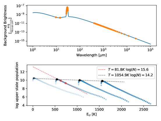
Figure 7: This figure demonstrates that a bright emission feature in the mid-infrared may explain the observed level populations. The top panel shows the input radiation field as a blue line, with orange dots showing the NaCl transitions. The narrow peak at 29 $\mu\textrm{m}$ is artificially added, and it may represent a broad dust emission feature. The bottom panel shows a level population diagram similar to Figure 6. The models include only v=0,1,2,3 because the collisional constants are limited to these states. The black dashed line shows a fit to the J=8 transitions of all vibrational states, yielding a high $\sim 1000$ K temperature. The red dashed line shows a fit to the observed $v=1$ lines, obtaining a much lower $\sim 100$ K temperature. The vertical scaling, the column density, is arbitrary, i.e., it does not represent a fit to the data; the optical depths of the observed lines range from $\sim 0.25$ to $\sim 1.5$.

(4) Ultraviolet excitation. The high vibrational and low rotational temperatures of the salt lines resemble the ‘sawtooth’ pattern observed for the rovibrational populations of $\textrm{H}_{2}$ toward the Orion bar photodissociation region. This pattern is explained by ultraviolet excitation into higher electronic states, followed by decay back to excited vibrational levels in the ground electronic state (Kaplan et al., 2017). $\textrm{H}_{2}$ rotational populations in the ground vibrational state are thermalized by collisions; UV excitation transposes this pattern into higher vibrational states.

Unfortunately, there are several problems applying this model to the salt lines. First, we find an abrupt decline in the populations of $v>6$ vibrational states, with weak or ambiguous detections of NaCl in the v=7 and v=8 levels, and nondetections for $v>9$. Unless there is some selection effect in the electronic de-excitation disfavoring higher vibrational states, it is difficult to explain this cutoff. Second, the lowest excited electronic energy levels for both NaCl and KCl are about 5 eV above the ground state, very close to the photodissociation threshold for these molecules (Zeiri & Balint-Kurti, 1983; Silver et al., 1986a), which may therefore be dissociated rather than excited by UV photons. Third, there may not be any UV radiation in the outer disk where these lines are detected. While UV emission may be produced in shocks in the outflow, and $\sim 5$ eV photons could be produced by the central $\sim 4000$ K photosphere (Testi et al., 2010), it is unclear whether it could penetrate into the disk where the salt emission is observed. Even a light haze of dust in the upper layers of the disk would likely shield the molecules from such illumination.

(5) Dust opacity. Finally, we consider the possibility that rotational temperatures, which are based on measurements of spectral lines over a wide frequency range, are underestimated because of greater dust extinction at high frequencies. Vibrational temperatures should be little affected by extinction because they are derived from lines in the same ALMA band that suffer similar dust attenuation.

Comparison of the observed line and continuum ratios across the bands suggests that dust extinction is not the dominant effect governing the rotational temperature. The KCl v=0 lines, which are the only vibrational state detected in all three observed bands, have similar peak brightnesses at $\sim 100$ and $\sim 345$ GHz ($T_{B,max}(\textrm{KCl v=0 13-12})=15.3\pm 0.9$ K and $T_{B,max}(\textrm{KCl v=0 45-44})=9.7\pm 1.8$ K). If the rotational excitation temperature $T_{ex}$ were comparable with the observed vibrational excitation temperatures $T_{vib}\sim 1000$ K, the 45-44 transition would be 9 times as bright as the 13-12 transition. If we assume a dust opacity index $\beta=2$, which is conservative in that it provides the greatest difference in extinction between the two frequencies, the dust opacities required to produce the observed line ratio are $\tau_{345\textrm{GHz}}=2.8$ and $\tau_{100\textrm{GHz}}=0.2$. These optical depths would result in a substantially ($\approx 4\times$) higher dust brightness at 0.85 $\mu\textrm{m}$ than at 3 mm, which is not observed.

Dust obscuration on sub-beam scales could preferentially block our view of some of the high frequency salt emission region, which would bias our measurements toward cooler rotational temperatures. However, the morphology of the line emission does not change with frequency, suggesting that this effect is negligible. Figure 8 shows the salt line images in each frequency band convolved to the same resolution, confirming that the morphological differences are minimal.

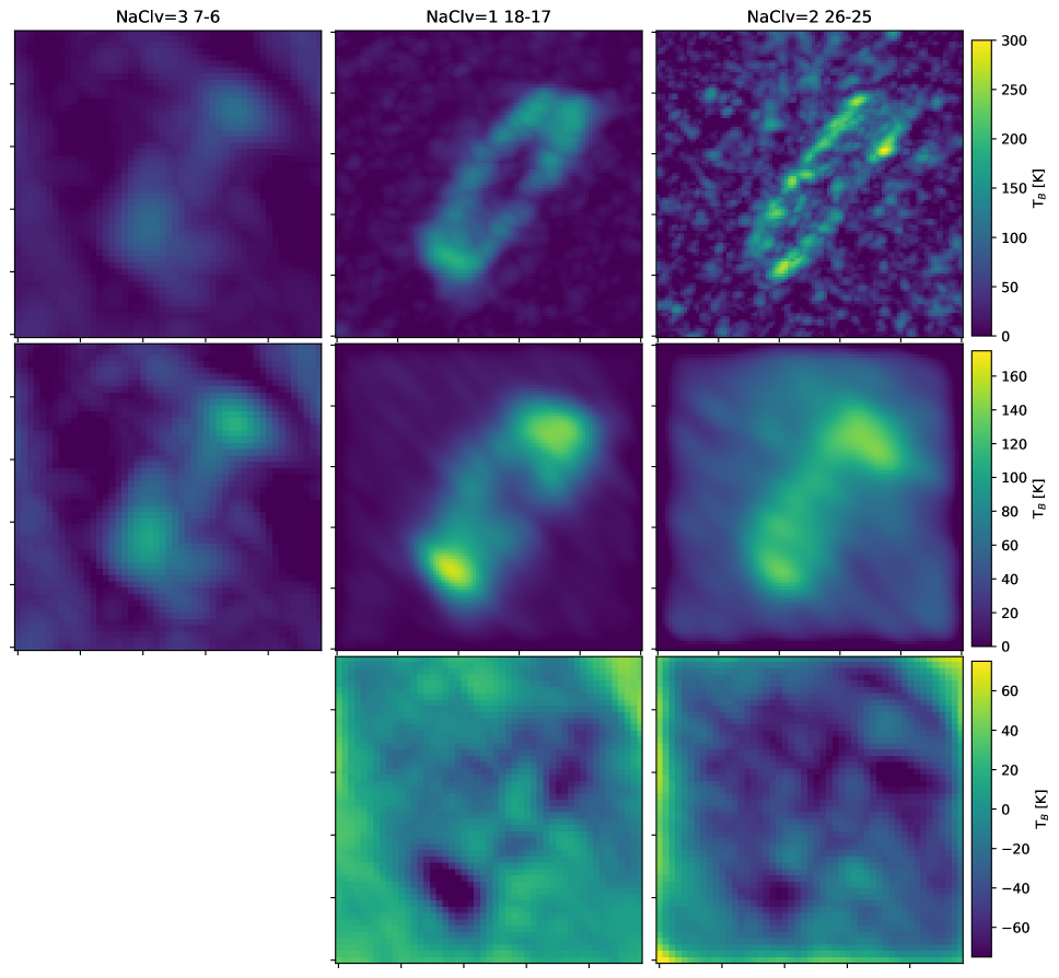
Figure 8: Comparison of three NaCl emission lines in different wavebands viewed at the same spatial resolution. The columns show, from left to right, NaCl v=3 J=7-6, NaCl v=1 J=18-17, and NaCl v=2 J=26-25, as in Figure 4. The top row shows these images in their native resolution, the middle shows them convolved to the resolution of the 3 mm band (note that the 3 mm band image is unchanged, but is repeated because the color scale has changed), and the bottom row shows the difference images $T_{B,3\mathrm{mm}}-T_{B,1.4\mathrm{mm}}$ and $T_{B,3\mathrm{mm}}-T_{B,0.87\mathrm{mm}}$.

We conclude that there is no simple model that explains the observed pattern of low rotational and high vibrational temperature.

3.3 What is producing gas-phase salts?

Sodium and potassium are rarely observed in the dense molecular interstellar medium. They are usually assumed to be rapidly incorporated into dust grains after being ejected from dying stars (e.g., Milam et al., 2007). Since we observe NaCl and KCl in the atmosphere of the disk, it is clear that there is a zone where either dust has not formed (which is not very likely in a protostellar system) or where dust is destroyed and returned to the gas phase. We argue that the dust must be destroyed almost immediately as it is launched into the disk-driven outflow (Hirota et al., 2017). We evaluate three scenarios for salt production: sputtering off of dust by high-energy particles, gas-phase formation from atomic gas, and thermal desorption.

(1) Sputtering: In the first scenario, NaCl and KCl molecules are sputtered from the grains. The most plausible means to achieve the energies required to sputter grains is with strong shocks (Schilke et al., 1997; Decin et al., 2016). In SrcI, it seems unlikely that there would be very strong shocks in the disk, but there are high-velocity shocks throughout the outflow. Bright SiO emission is observed in the inner part of the outflow (i.e., within $<100$ AU of SrcI), suggesting that grains are efficiently destroyed there. Without knowing the grain structure, however, it is unclear whether high-energy particles capable of destroying the grain cores are present.

Since the salts are detected close to but above the disk midplane, the grains must be sputtered very rapidly after being launched from the disk surface. The lack of salt and SiO emission in the disk midplane may be because these molecules are not in the gas phase at all in the midplane. Alternatively, radiative transfer can explain their non-detection, i.e., if the continuum background is the same intensity as the emission lines.

In this model, both SiO and the salts are in the gas phase above the disk midplane. However, while low-J SiO lines are seen throughout the outflow at very high elevations above the disk, the salt lines are limited to $\lesssim 30$ AU from the midplane. Even the low-J salt lines, which can be excited at the same modest densities required to excite SiO ($n\sim 10^{4}$ to $10^{6}$ $\textrm{cm}^{-3}$), are not observed at high elevations. Excitation therefore cannot explain the morphological difference between SiO and the salts, and instead we infer that they are chemically distinct. Possible explanations are that the salts deplete back onto grains as they are entrained in the outflow, they react to form other molecules, or they dissociate into atomic form while SiO remains molecular.

(2) Gas-phase formation: Gas-phase formation of NaCl and KCl is possible from ionized Na and K. Potassium and sodium have similar first ionization potentials at 4.34 and 5.14 eV, respectively. These atoms would be nearly fully ionized between 1500-2000 K at a density of $10^{6}$ $\textrm{cm}^{-3}$ (aluminum has a higher first ionization potential of 5.99 eV, and so is ionized at a few hundred K higher temperatures than sodium). These ions react with HCl to form NaCl and KCl. However, at present, only the inner $<20$ AU region, which is currently unresolved, clearly reaches such high temperatures.

For gas-phase formation to be a significant process, then, either material in that hot inner region is being transported outward, which seems unlikely since there is a bulk outflow lifting material off of the disk, or the disk was previously substantially warmer. Under the dynamical formation scenario of the disk, in which it is the remnant of a previously larger disk from the SrcI-BN interaction (Bally et al., 2017; Luhman et al., 2017; Kim et al., 2018), energy was released as the disk re-settled into its current apparently smooth state, which could have resulted in much higher gas temperatures over the last few hundred years. This scenario would imply that the observable state of NaCl and KCl is very short lived, as these molecules are in the process of depleting onto grains. While plausible, there are many processes that need to coincide perfectly in this scenario (disk temperature history, gas density, gas-phase formation rates), so we favor the dust destruction hypotheses.

We note that, if the formation rates of NaCl and KCl are very high, it is possible that the vibrational excitation observed is from the chemical energy of formation. However, because of the short expected lifetimes of the vibrationally excited states, we regard this explanation for the excitation as very unlikely.

(3) Thermal desorption from grain surfaces Decin et al. (2016) presented a model for the gas-phase abundance of NaCl in which it is thermally desorbed from grains at grain temperatures between 100 and 300 K, depending on the unknown binding energy of NaCl with the grain surface. Since we expect grain temperatures $T>150$ K in the NaCl emission region (see Section 3.1), this model hints that simple grain heating is enough to explain the high gas-phase abundances of NaCl observed. Since NaCl is not observed within $r<30AU$, though, it must be dissociated at smaller radii, which most likely requires a substantial UV field within that radius in the wavelength range $912\mathrm{\AA}<\lambda<3000\mathrm{\AA}$ (Silver et al., 1986b).

This model is plausible, though it relies on unknown physical parameters. Additionally, while a 4000 K stellar atmosphere (Testi et al., 2010) produces non-negligible radiation short of 3000 Å, it is unclear whether that radiation can propagate to the part of the disk where the salts are observed, since small dust grains may pervade the system.

3.4 Other salts

While NaCl and KCl are clearly detected here, there are also several transitions of AlCl and AlF in our observational bands that were not detected. Cernicharo & Guelin (1987) detected these transitions at comparable brightness to NaCl and KCl in IRC+10216. The lack of AlCl may be because SrcI’s disk is oxygen-rich, and aluminum is locked into AlOH, as suggested in the Cherchneff (2012) model. Indeed, the tentative detection of AlO in our spectra supports this conclusion.

3.5 Isotopologue abundances

With several transitions of each of the observed isotopologues, we can in principle measure the relative abundance of the various isotopes. However, because of the uncertainties in the excitation above, these measurements should be taken with a grain of salt.

The ³⁷Cl abundance can be measured by comparing the intensity of the NaCl and Na³⁷Cl v=3 J=7-6, v=4 J=8-7 and J=7-6, and v=5 J=7-6 lines assuming they are optically thin. The ratio ³⁵/³⁷Cl is $r=1.4\pm 0.4$. The KCl v=0 J=45-44 line gives a ${}^{35}/^{37}$Cl ratio $r=0.8$. Agúndez et al. (2012) measured this ratio to be $r=2.9\pm 0.3$ in IRC+10216, and Highberger et al. (2003) reported a ratio of 2.1 $\pm$ 0.8 in CRL 2688. Our measurement is somewhat lower, but should be regarded as consistent at least until we can obtain more accurate column density measurements.

We only have one commonly observed ⁴¹KCl / ³⁹KCl line, v=0 J=13-12, which has a ratio ${}^{39}/^{41}$ $r=2.4$.

3.6 Future prospects

The detection of these refractory species in the gas phase in the atmosphere of SrcI’s disk hints that other refractory molecules may be present, which could enable their first detection in the ISM (e.g., such rare species as FeO and FeS), and may enable direct measurements of the metallicity in star-forming gas.

The observed NaCl and KCl transitions uniquely trace the disk, unlike most other molecules observed in the ISM that are bright and abundant in hot cores like Sgr B2 (Nummelin et al., 1998; Belloche et al., 2013). These lines therefore potentially represent tracers that can uniquely trace high-mass disks, making them extremely valuable probes of early-stage high-mass star formation, at least at distances where the salt-emitting regions can be resolved. However, it remains unclear whether SrcI is a unique source or is representative of the class of high-mass protostars with disks; if the latter, these lines and potentially many others can be used to probe the radiation environment of extremely embedded high-mass protostars. An obvious next step is to search for these lines in other resolved disks around high-mass protostars (e.g., HH80/81; Girart et al., 2017). These species are particularly interesting for future millimeter and centimeter wavelength observatories like the ngVLA and SKA, since they have lower-J transitions into the few centimeter range, wavelengths at which the dust is very likely to be optically thin even in the inner few AU of a disk.

The detection of these species with substantial population in vibrationally excited states highlights the need for laboratory work to measure such transitions in known astronomical molecular species. Indeed, prior work on vibrational excitation in modeling and assigned vibrationally excited ethyl cyanide in ALMA observations of Orion-KL revealed that even when catalogs for these states are available, they are often incomplete (Fortman et al., 2012).

Table 7: Parameters of NaCl lines obtained with Gaussian fits

Ju	Jl	Frequency	Velocity	Amplitude	$\int T_{A}dv$	EU
		$\mathrm{GHz}$	$\mathrm{km\,s^{-1}}$	$\mathrm{K}$	$\mathrm{K\,km\,s^{-1}}$	$\mathrm{K}$
$v=1$
26	25	335.50656	5.5 (0.1)	29.1 (0.8)	339.9 (5.4)	737.2
18	17	232.50998	5.4 (0.2)	23.9 (0.7)	396.6 (6.7)	625.7
$v=2$
17	16	217.98023	5.2 (0.1)	19.3 (0.4)	267.8 (3.6)	1128.4
18	17	230.77917	5.6 (0.1)	19.3 (0.4)	297.7 (3.7)	1139.5
26	25	333.00729	7.4 (0.3)	21.7 (0.9)	352.2 (8.9)	1250.2
27	26	345.76204	0.2 (0.9)	11.5 (1.9)	136.4 (13.8)	1266.8
$v=3$
7	6	89.15011	3.8 (0.5)	14.1 (1.1)	183.1 (9.0)	1561.0
$v=4$
7	6	88.48549	3.8 (0.7)	11.4 (1.0)	185.4 (10.5)	2065.5
8	7	101.12183	3.1 (0.3)	15.5 (0.8)	214.1 (7.0)	2070.4
$v=5$
8	7	100.36722	3.7 (0.5)	10.0 (0.9)	122.3 (6.6)	2570.0
7	6	87.82519	4.5 (0.6)	11.6 (1.1)	173.8 (9.9)	2565.2
$v=6$
8	7	99.61753	4.4 (0.7)	7.7 (0.9)	100.0 (6.8)	3064.8
7	6	87.16921	3.4 (1.2)	7.2 (1.8)	73.9 (11.4)	3060.0

Table 8: Parameters of Na³⁷Cl lines obtained with Gaussian fits

Ju	Jl	Frequency	Velocity	Amplitude	$\int T_{A}dv$	EU
		$\mathrm{GHz}$	$\mathrm{km\,s^{-1}}$	$\mathrm{K}$	$\mathrm{K\,km\,s^{-1}}$	$\mathrm{K}$
$v=0$
7	6	89.22011	4.3 (0.4)	18.2 (1.2)	230.2 (8.9)	17.1
18	17	229.24605	4.8 (0.1)	21.4 (0.4)	251.5 (3.2)	104.6
$v=1$
17	16	214.93871	4.8 (0.4)	18.7 (1.2)	217.3 (8.8)	607.0
8	7	101.21188	4.6 (0.3)	19.7 (0.8)	281.1 (7.1)	536.0
$v=2$
8	7	100.46695	5.3 (0.4)	15.6 (0.7)	307.2 (9.0)	1045.0
7	6	87.91232	4.3 (0.6)	13.1 (1.1)	205.3 (10.2)	1040.1
$v=3$
7	6	87.26464	2.9 (1.0)	9.0 (1.7)	102.0 (11.9)	1544.3
8	7	99.72675	3.7 (0.4)	14.0 (0.8)	203.9 (7.3)	1549.1
$v=4$
7	6	86.62109	-2.1 (1.1)	13.0 (1.4)	265.3 (19.6)	2043.6
8	7	98.99127	4.6 (1.1)	8.2 (1.9)	86.3 (11.9)	2048.4
27	26	333.45906	5.5 (0.5)	10.9 (1.0)	130.9 (7.3)	2251.3
$v=5$
19	18	233.16920	5.2 (0.5)	7.4 (0.8)	72.8 (5.0)	2633.6
7	6	85.98167	5.2 (1.2)	8.1 (1.7)	99.9 (12.6)	2538.2

Table 9: Parameters of KCl lines obtained with Gaussian fits

Ju	Jl	Frequency	Velocity	Amplitude	$\int T_{A}dv$	EU
		$\mathrm{GHz}$	$\mathrm{km\,s^{-1}}$	$\mathrm{K}$	$\mathrm{K\,km\,s^{-1}}$	$\mathrm{K}$
$v=0$
28	27	215.00828	5.5 (0.6)	10.4 (1.3)	113.1 (8.4)	149.7
30	29	230.32064	4.6 (0.2)	14.4 (0.4)	171.2 (3.2)	171.4
45	44	344.82061	2.5 (1.1)	9.7 (1.8)	120.0 (13.9)	381.2
13	12	99.92952	4.0 (0.3)	15.3 (0.9)	183.8 (6.5)	33.6
$v=1$
13	12	99.31663	3.9 (1.0)	8.3 (2.0)	75.2 (11.0)	432.6
44	43	335.13396	3.3 (0.3)	14.1 (0.8)	143.3 (5.0)	761.7
$v=2$
44	43	333.06770	3.9 (0.5)	11.4 (1.0)	135.6 (7.3)	1155.3
13	12	98.70595	2.0 (0.8)	14.2 (1.5)	229.2 (15.2)	828.3
$v=3$
31	30	233.60570	4.8 (0.7)	6.0 (0.8)	64.1 (5.2)	1367.1
13	12	98.09753	6.1 (1.1)	9.2 (1.7)	116.3 (13.2)	1220.6
29	28	218.57971	4.4 (0.4)	5.0 (0.6)	40.8 (2.8)	1345.1
$v=4$
31	30	232.16185	4.6 (0.6)	6.6 (0.8)	65.0 (5.0)	1755.1
13	12	97.49133	8.0 (2.1)	6.1 (1.5)	107.3 (18.0)	1609.5
29	28	217.22891	-0.3 (0.6)	3.5 (0.6)	28.4 (2.8)	1733.2
$v=5$
45	44	334.29930	2.1 (0.3)	42.9 (0.5)	1550.0 (21.5)	2332.2
31	30	230.72399	5.3 (0.4)	5.2 (0.5)	56.2 (3.1)	2139.8
29	28	215.88373	6.3 (2.1)	3.0 (1.3)	32.6 (8.4)	2118.0
$v=6$
31	30	229.29217	6.0 (0.5)	4.1 (0.5)	32.6 (2.6)	2521.2
47	46	346.87489	0.7 (1.1)	4.4 (0.8)	61.1 (6.8)	2745.3
29	28	214.54412	6.3 (1.9)	3.4 (1.3)	37.0 (8.5)	2499.6
$v=7$
47	46	344.71476	4.7 (3.1)	5.1 (1.4)	118.3 (23.7)	3122.1

Table 10: Parameters of K³⁷Cl lines obtained with Gaussian fits

Ju	Jl	Frequency	Velocity	Amplitude	$\int T_{A}dv$	EU
		$\mathrm{GHz}$	$\mathrm{km\,s^{-1}}$	$\mathrm{K}$	$\mathrm{K\,km\,s^{-1}}$	$\mathrm{K}$
$v=0$
45	44	335.05072	7.0 (0.4)	12.6 (0.7)	182.0 (6.1)	370.4
$v=1$
47	46	347.71265	4.6 (0.5)	7.4 (1.0)	63.7 (5.1)	794.8
31	30	229.81880	5.5 (0.3)	7.2 (0.4)	86.9 (3.2)	570.2
$v=2$
12	11	88.54307	5.2 (1.5)	4.3 (1.2)	50.1 (8.5)	811.5
$v=3$
12	11	88.00523	4.4 (1.4)	5.6 (1.0)	90.3 (10.4)	1198.3
$v=4$
32	31	232.90755	5.0 (1.1)	4.0 (0.7)	51.7 (5.7)	1739.2
$v=6$
32	31	230.07072	3.9 (1.3)	1.9 (0.4)	25.0 (3.4)	2494.7
30	29	215.73679	5.9 (2.8)	1.9 (1.5)	13.9 (7.0)	2473.0

Table 11: Parameters of ⁴¹KCl lines obtained with Gaussian fits

Ju	Jl	Frequency	Velocity	Amplitude	$\int T_{A}dv$	EU
		$\mathrm{GHz}$	$\mathrm{km\,s^{-1}}$	$\mathrm{K}$	$\mathrm{K\,km\,s^{-1}}$	$\mathrm{K}$
$v=0$
29	28	217.54317	5.5 (0.7)	4.5 (0.4)	72.9 (4.0)	156.7
13	12	97.62809	4.7 (2.5)	6.5 (1.3)	162.6 (24.7)	32.8
$v=1$
45	44	334.85439	5.1 (0.6)	5.2 (1.0)	36.3 (4.2)	764.9
$v=2$
31	30	229.68227	2.7 (0.6)	9.6 (0.3)	319.8 (10.2)	962.5
12	11	89.03129	- (-)	- (-)	- (-)	813.8

Table 12: Parameters of ⁴¹K³⁷Cl lines obtained with Gaussian fits

Ju	Jl	Frequency	Velocity	Amplitude	$\int T_{A}dv$	EU
		$\mathrm{GHz}$	$\mathrm{km\,s^{-1}}$	$\mathrm{K}$	$\mathrm{K\,km\,s^{-1}}$	$\mathrm{K}$
$v=7$
48	47	334.32791	-9.5 (0.0)	24.5 (0.9)	347.9 (8.2)	3049.3

4 Conclusions

We have identified many transitions of NaCl, KCl, and their isotopologues in the disk of SrcI. These lines trace material very near the surface of the disk, providing a uniquely powerful probe of the disk kinematics and physical conditions.

Despite the wide range of transitions observed, the excitation mechanism and conditions remain uncertain. Further observations of lower-energy vibrational and rotational states of these molecules will help distinguish between radiative and collisional excitation scenarios and will either provide direct measurements of the density or the radiation field in the 30-60 AU region around SrcI.

The narrow vertical extent of the salt emission indicates that dust is destroyed nearly immediately after being raised from the surface of the disk. This morphology hints that immediate dust destruction is an integral part of the outflow driving process.

Given the rarity of these molecules, if they can be detected elsewhere, they will serve as a powerful and unique probe of local conditions. They may be the best available molecular tool to find disks around high-mass protostars and measure their kinematics.

References

- Agúndez et al. (2012) Agúndez, M., Fonfría, J. P., Cernicharo, J., et al. 2012, A&A, 543, A48, doi: 10.1051/0004-6361/201218963
- Astropy Collaboration et al. (2013) Astropy Collaboration, Robitaille, T. P., Tollerud, E. J., et al. 2013, A&A, 558, A33, doi: 10.1051/0004-6361/201322068
- Báez-Rubio et al. (2018) Báez-Rubio, A., Jiménez-Serra, I., Martín-Pintado, J., Zhang, Q., & Curiel, S. 2018, ApJ, 853, 4, doi: 10.3847/1538-4357/aaa24b
- Bally et al. (2017) Bally, J., Ginsburg, A., Arce, H., et al. 2017, ApJ, 837, 60, doi: 10.3847/1538-4357/aa5c8b
- Barton et al. (2014) Barton, E. J., Chiu, C., Golpayegani, S., et al. 2014, MNRAS, 442, 1821, doi: 10.1093/mnras/stu944
- Belloche et al. (2013) Belloche, A., Müller, H. S. P., Menten, K. M., Schilke, P., & Comito, C. 2013, ArXiv e-prints. https://arxiv.org/abs/1308.5062
- Bergin & Tafalla (2007) Bergin, E. A., & Tafalla, M. 2007, ARA&A, 45, 339, doi: 10.1146/annurev.astro.45.071206.100404
- Cabezas et al. (2016) Cabezas, C., Cernicharo, J., Quintana-Lacaci, G., et al. 2016, ApJ, 825, 150, doi: 10.3847/0004-637X/825/2/150
- Caris et al. (2004) Caris, M., Lewen, F., Müller, H. S. P., & Winnewisser, G. 2004, Journal of Molecular Structure, 695, 243, doi: 10.1016/j.molstruc.2003.11.010
- Caris et al. (2002) Caris, M., Lewen, F., & Winnewisser, G. 2002, Zeitschrift Naturforschung Teil A, 57, 663, doi: 10.1515/zna-2002-0805
- Cernicharo & Guelin (1987) Cernicharo, J., & Guelin, M. 1987, A&A, 183, L10
- Cesaroni et al. (2017) Cesaroni, R., Sánchez-Monge, Á., Beltrán, M. T., et al. 2017, A&A, 602, A59, doi: 10.1051/0004-6361/201630184
- Cherchneff (2012) Cherchneff, I. 2012, A&A, 545, A12, doi: 10.1051/0004-6361/201118542
- Chiang & Goldreich (1997) Chiang, E. I., & Goldreich, P. 1997, ApJ, 490, 368, doi: 10.1086/304869
- Decin et al. (2016) Decin, L., Richards, A. M. S., Millar, T. J., et al. 2016, A&A, 592, A76, doi: 10.1051/0004-6361/201527934
- Dickinson & Richards (1975) Dickinson, A. S., & Richards, D. 1975, in Physics of Electronic and Atomic Collisions: ICPEAC IX, ed. J. S. Risley & R. Geballe, 291
- Fortman et al. (2012) Fortman, S. M., McMillan, J. P., Neese, C. F., et al. 2012, Journal of Molecular Spectroscopy, 280, 11, doi: 10.1016/j.jms.2012.08.002
- Ginsburg et al. (2018) Ginsburg, A., Bally, J., Goddi, C., Plambeck, R., & Wright, M. 2018, ApJ, 860, 119, doi: 10.3847/1538-4357/aac205
- Ginsburg et al. (2018a) Ginsburg, A., Robitaille, T., Koch, E., et al. 2018a, radio-astro-tools/spectral-cube, v0.4.3, Zenodo, doi: 10.5281/zenodo.1213217. https://doi.org/10.5281/zenodo.1213217
- Ginsburg et al. (2018b) Ginsburg, A., Sipocz, B., Parikh, M., et al. 2018b, astropy/astroquery, v0.3.8, Zenodo, doi: 10.5281/zenodo.1234036. https://doi.org/10.5281/zenodo.1234036
- Girart et al. (2017) Girart, J. M., Estalella, R., Fernández-López, M., et al. 2017, ApJ, 847, 58, doi: 10.3847/1538-4357/aa81c9
- Goddi et al. (2018) Goddi, C., Ginsburg, A., Maud, L., Zhang, Q., & Zapata, L. 2018, ArXiv e-prints. https://arxiv.org/abs/1805.05364
- Goddi et al. (2010) Goddi, C., Greenhill, L., Humphreys, E., Matthews, L., & Chandler, C. 2010, Highlights of Astronomy, 15, 750, doi: 10.1017/S174392131001135X
- Goddi et al. (2009) Goddi, C., Greenhill, L. J., Humphreys, E. M. L., et al. 2009, ApJ, 691, 1254, doi: 10.1088/0004-637X/691/2/1254
- Greenhill et al. (2013) Greenhill, L. J., Goddi, C., Chandler, C. J., Matthews, L. D., & Humphreys, E. M. L. 2013, ApJ, 770, L32, doi: 10.1088/2041-8205/770/2/L32
- Grossschedl et al. (2018) Grossschedl, J. E., Alves, J., Meingast, S., et al. 2018, ArXiv e-prints. https://arxiv.org/abs/1808.05952
- Herwig (2005) Herwig, F. 2005, ARA&A, 43, 435, doi: 10.1146/annurev.astro.43.072103.150600
- Highberger et al. (2003) Highberger, J. L., Thomson, K. J., Young, P. A., Arnett, D., & Ziurys, L. M. 2003, ApJ, 593, 393, doi: 10.1086/376446
- Hirota et al. (2014) Hirota, T., Kim, M. K., Kurono, Y., & Honma, M. 2014, ApJ, 782, L28, doi: 10.1088/2041-8205/782/2/L28
- Hirota et al. (2017) Hirota, T., Machida, M. N., Matsushita, Y., et al. 2017, Nature Astronomy, 1, 0146, doi: 10.1038/s41550-017-0146
- Hunter (2007) Hunter, J. D. 2007, Matplotlib: A 2D Graphics Environment, Computing in Science and Engineering, 9, 90-95
- Jones et al. (2001–) Jones, E., Oliphant, T., Peterson, P., et al. 2001–, SciPy: Open source scientific tools for Python, http://www.scipy.org/
- Kamiński et al. (2013) Kamiński, T., Gottlieb, C. A., Young, K. H., Menten, K. M., & Patel, N. A. 2013, ApJS, 209, 38, doi: 10.1088/0067-0049/209/2/38
- Kaplan et al. (2017) Kaplan, K. F., Dinerstein, H. L., Oh, H., et al. 2017, ApJ, 838, 152, doi: 10.3847/1538-4357/aa5b9f
- Kim et al. (2018) Kim, D., Lu, J. R., Konopacky, Q., et al. 2018, arXiv e-prints. https://arxiv.org/abs/1812.04134
- Koch et al. (2018) Koch, E., Ginsburg, A., AKL, et al. 2018, keflavich/radio_beam, v0.0 prerelease, Zenodo, doi: 10.5281/zenodo.1181879. https://doi.org/10.5281/zenodo.1181879
- Lovas et al. (2005) Lovas, F. J., Tiemann, E., Coursey, J. S., et al. 2005, NIST Chemistry WebBook, NIST Standard Reference Database Number 114 No. 114 (https://dx.doi.org/10.18434/T4T59X: NIST Physical Measurement Laboratory)
- Luhman et al. (2017) Luhman, K. L., Robberto, M., Tan, J. C., et al. 2017, ApJ, 838, L3, doi: 10.3847/2041-8213/aa5ff6
- Matthews et al. (2010) Matthews, L. D., Greenhill, L. J., Goddi, C., et al. 2010, ApJ, 708, 80, doi: 10.1088/0004-637X/708/1/80
- McGuire (2018) McGuire, B. A. 2018, ApJS, 239, 17, doi: 10.3847/1538-4365/aae5d2
- McMullin et al. (2007) McMullin, J. P., Waters, B., Schiebel, D., Young, W., & Golap, K. 2007, in Astronomical Society of the Pacific Conference Series, Vol. 376, Astronomical Data Analysis Software and Systems XVI, ed. R. A. Shaw, F. Hill, & D. J. Bell, 127
- Milam et al. (2007) Milam, S. N., Apponi, A. J., Woolf, N. J., & Ziurys, L. M. 2007, ApJ, 668, L131, doi: 10.1086/522928
- Molster & Kemper (2005) Molster, F., & Kemper, C. 2005, Space Sci. Rev., 119, 3, doi: 10.1007/s11214-005-8066-x
- Müller et al. (2005) Müller, H. S. P., Schlöder, F., Stutzki, J., et al. 2005, in IAU Symposium, Vol. 235, IAU Symposium, 62P
- Niederhofer et al. (2012) Niederhofer, F., Humphreys, E. M. L., & Goddi, C. 2012, A&A, 548, A69, doi: 10.1051/0004-6361/201220292
- Nummelin et al. (1998) Nummelin, A., Bergman, P., Hjalmarson, Å., et al. 1998, ApJS, 117, 427, doi: 10.1086/313126
- Oliphant (2006) Oliphant, T. E. 2006, A guide to NumPy, Trelgol Publishing
- Pickett et al. (1998) Pickett, H. M., Poynter, R. L., Cohen, E. A., et al. 1998, J. Quant. Spec. Radiat. Transf., 60, 883, doi: 10.1016/S0022-4073(98)00091-0
- Plambeck & Wright (2016) Plambeck, R. L., & Wright, M. C. H. 2016, ApJ, 833, 219, doi: 10.3847/1538-4357/833/2/219
- Plambeck et al. (2009) Plambeck, R. L., Wright, M. C. H., Friedel, D. N., et al. 2009, ApJ, 704, L25, doi: 10.1088/0004-637X/704/1/L25
- Quintana-Lacaci et al. (2016) Quintana-Lacaci, G., Cernicharo, J., Agúndez, M., et al. 2016, ApJ, 818, 192, doi: 10.3847/0004-637X/818/2/192
- Sánchez Contreras et al. (2018) Sánchez Contreras, C., Alcolea, J., Castro-Carrizo, A., et al. 2018, ArXiv e-prints. https://arxiv.org/abs/1809.00619
- Schilke et al. (1997) Schilke, P., Walmsley, C. M., Pineau des Forets, G., & Flower, D. R. 1997, A&A, 321, 293
- Silver et al. (1986a) Silver, J. A., Worsnop, D. R., Freedman, A., & Kolb, C. E. 1986a, J. Chem. Phys., 84, 4378, doi: 10.1063/1.450060
- Silver et al. (1986b) —. 1986b, J. Chem. Phys., 84, 4378, doi: 10.1063/1.450060
- Testi et al. (2010) Testi, L., Tan, J. C., & Palla, F. 2010, A&A, 522, A44, doi: 10.1051/0004-6361/201014497
- van der Tak et al. (2007) van der Tak, F. F. S., Black, J. H., Schöier, F. L., Jansen, D. J., & van Dishoeck, E. F. 2007, A&A, 468, 627, doi: 10.1051/0004-6361:20066820
- Zack et al. (2011) Zack, L. N., Halfen, D. T., & Ziurys, L. M. 2011, ApJ, 733, L36, doi: 10.1088/2041-8205/733/2/L36
- Zeiri & Balint-Kurti (1983) Zeiri, Y., & Balint-Kurti, G. G. 1983, Journal of Molecular Spectroscopy, 99, 1, doi: 10.1016/0022-2852(83)90288-6